APPLICATION OF EFFICIENT EXTERNAL MEMORY ALGORITHMS TO

SIMULATED WEB GRAPHS

by

DONGSHENG CHE

(Under the direction of Robert W. Robinson)

ABSTRACT

The Web graph is a graph of the World-Wide Web (WWW), with Web pages represented

by nodes and hyperlinks represented by directed edges. In the past decade, the WWW has

spawned a sharing and dissemination of information on an unprecedented scale, and since

then much research has focused on crawling strategies used by search engines. Recent

study has shown that breadth first search crawling, one of the current crawling strategies,

yields high quality pages. However, very little has been done on increasing the overall

download rate when using breadth-first search crawling in the face of the “massive”

character of the Web graph. Problems for massive data sets can be solved either by

storing data sets in a huge main memory, or by storing data sets in external memory but

with I/O efficient techniques. The goal of our research is to study how to reduce breadth-

first search time for crawling by using I/O efficient techniques. We used data structures

provided by LEDA-SM to store massive data sets of our simulated Web graphs, and run

BFS on these generated graphs. The simulated Web graphs share important properties

with the real Web graph, i.e., the degree distributions follow the same power laws, and

random-start BFS traversals exhibit sharply bimodal behavior. The results indicate that

the LEDA-SM system is useful for the Web graph computations, especially on machines

with modest amounts of main memory.

INDEX WORDS: web graph, massive data sets, LEDA-SM, breadth first search,

power law, secondary memory model.

APPLICATION OF EFFICIENT EXTERNAL MEMORY ALGORITHMS TO

SIMULATED WEB GRAPHS

by

DONGSHENG CHE

B.Ag. Zhejiang Forestry College, P.R. China, 1992

M.S. Beijing Forestry University, P.R. China, 1995

M.S. The University of Georgia, 2000

A Thesis Submitted to the Graduate Faculty of The University of Georgia in Partial

Fulfillment of the Requirements for the Degree

MASTER OF SCIENCE

ATHENS, GEORGIA

2002

© 2002

Dongsheng Che

All Rights Reserved

APPLICATION OF EFFICIENT EXTERNAL MEMORY ALGORITHMS TO

SIMULATED WEB GRAPHS

by

DONGSHENG CHE

Major Professor: Robert W. Robinson

Committee: Ismailcem B. Arpinar Liming Cai

Electronic Version Approved: Maureen Grasso Dean of the Graduate School The University of Georgia December 2002

iv

DEDICATION

To my beloved, late parents

v

ACKNOWLEDGEMENTS

I would like to express sincere thanks to my major professor, Dr. Robert W.

Robinson, for his friendly advice, honest criticism and endless patience throughout my

degree program. Without Dr. Robinson's advice and effort, completion of this thesis

would have been impossible.

I would also like to thank Dr. Budak Arpinar and Dr. Liming Cai for serving on

my thesis committee. Special gratitude must go to Dr. Liming Cai for providing his

computing facilities for me to use. I appreciate the faculty, staff, and graduate students of

the Department of Computer Science for their cooperation and help.

Finally, my greatest thanks must go to my beloved girlfriend, Anna, for her love,

sacrifice, patience and support throughout my program study.

vi

TABLE OF CONTENTS

Page

ACKNOWLEDGEMENTS................................................................................................ v

LIST OF TABLES............................................................................................................vii

LIST OF FIGURES..........................................................................................................viii

CHAPTER

1 INTRODUCTION............................................................................................. 1

1.1 Graph definitions.................................................................................. 1

1.2 The structure of the Web graph ............................................................ 3

1.3 Crawling strategies............................................................................... 7

1.4 Overview of research on secondary memory computation .................. 9

1.5 The goal of the research...................................................................... 12

2 LEDA-SM ....................................................................................................... 14

2.1 Architecture of LEDA-SM ................................................................. 14

2.2 The kernel structure of LEDA-SM ..................................................... 15

2.3 External graph data structures and BFS............................................. 24

3 SIMULATION OF THE WEB GRAPH......................................................... 32

3.1 Generating a model of the Web graph................................................ 32

3.2 BFS on simulated Web graphs .......................................................... 39

4 CONCLUSIONS AND FUTURE WORK ..................................................... 40

REFERENCES.................................................................................................................. 42

vii

LIST OF TABLES

Page

Table 2.1: LEDA-SM Configuration File. ........................................................................ 21

Table 3.1: Parameters of the Simulated Web Graph and BFS Results............................. 39

viii

LIST OF FIGURES

Page

Figure 1.1: (a) A Random Graph with 4 Nodes, (b) A Complete Graph with 6 Nodes...... 2

Figure 1.2: Breadth First Search (BFS) Showing Visitation Order .................................... 3

Figure 1.3: In-degrees Follow a Power Law with Exponent 2.1......................................... 4

Figure 1.4: Out-degrees Follow a Power Law with Exponent 2.72.................................... 5

Figure 1.5: Components of the Web Macroscopic Structure ............................................. 6

Figure 1.6: The Secondary Memory Model of Vitter and Shriver.................................... 10

Figure 2.1: Architecture of LEDA-SM ............................................................................. 15

Figure 2.2: UML Diagram of LEDA-SM Kernel ............................................................. 16

Figure 2.3: UML Diagram of the Concrete Kernel without Class name_server .............. 19

Figure 2.4: Data Layout of node_container ...................................................................... 26

Figure 2.5: Data Layout of edge_container ...................................................................... 27

Figure 2.6: Comparison of LEDA BFS and LEDA-SM BFS with an Internal Bit Array on

Random Graphs with 100,000 Nodes and m Edges........................................... 30

Figure 2.7: Comparison of LEDA BFS and LEDA-SM BFS with an Internal Bit Array on

Complete Graphs with n Nodes......................................................................... 31

Figure 3.1: The Source Node Array Source with Length m.............................................. 35

Figure 3.2: The Temporary Array A of Type ext_array and Length n ............................. 36

Figure 3.3: The Target Node Array Target with Length m............................................... 37

1

CHAPTER 1

INTRODUCTION

1.1 Graph definitions

A graph G consists of a finite non-empty set of nodes, denoted V(G) and a finite

set of edges (or arcs), denoted E(G). Each edge is a pair of distinct vertices, which may

be ordered or unordered. In this thesis ordered edges are called arcs. A directed graph is

a graph where each edge is an arc. An arc represents a directed connection from u to v,

where u is usually called the source node, while v is called the target node. The out-

degree of a node u is the number of distinct arcs (u, v1) ... (u, vk) (i. e., the number of links

from u), and the in-degree is the number of distinct arcs (v1, u) ... (vk, u) (i. e., the number

of links to u). A path from node u to node v is a sequence of arcs (u, u1), (u1, u2) ... (uk,

v). One can follow such a sequence of arcs to "walk" through the graph from u to v. Note

that a path from u to v does not imply a path from v to u. The distance from u to v is the

minimum number of edges in such a path. If no path exists, the distance from u to v is

defined to be infinity. If (u, v) is an arc, then the distance from u to v is 1.

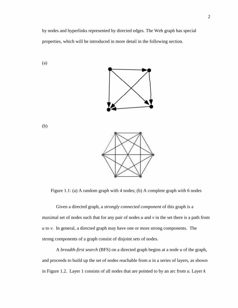
A random graph is a graph in which source nodes and target nodes for arcs are

picked randomly from the set of nodes, as shown in Figure 1.1(a). A complete graph is a

graph a simple graph in which every pair of nodes is adjacent as shown in Figure 1.1(b).

A Web graph is a graph of the World-Wide Web (WWW), with Web pages represented

2

by nodes and hyperlinks represented by directed edges. The Web graph has special

properties, which will be introduced in more detail in the following section.

(a)

(b)

Figure 1.1: (a) A random graph with 4 nodes; (b) A complete graph with 6 nodes

Given a directed graph, a strongly connected component of this graph is a

maximal set of nodes such that for any pair of nodes u and v in the set there is a path from

u to v. In general, a directed graph may have one or more strong components. The

strong components of a graph consist of disjoint sets of nodes.

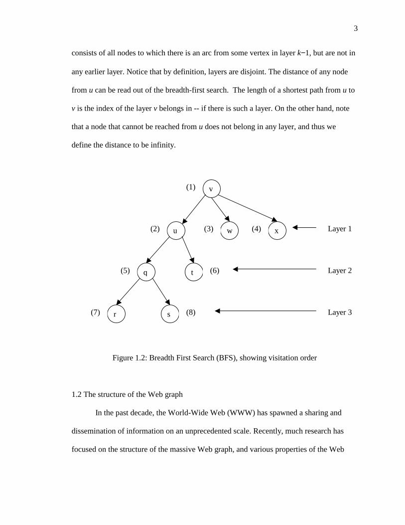
A breadth-first search (BFS) on a directed graph begins at a node u of the graph,

and proceeds to build up the set of nodes reachable from u in a series of layers, as shown

in Figure 1.2. Layer 1 consists of all nodes that are pointed to by an arc from u. Layer k

3

consists of all nodes to which there is an arc from some vertex in layer k−1, but are not in

any earlier layer. Notice that by definition, layers are disjoint. The distance of any node

from u can be read out of the breadth-first search. The length of a shortest path from u to

v is the index of the layer v belongs in -- if there is such a layer. On the other hand, note

that a node that cannot be reached from u does not belong in any layer, and thus we

define the distance to be infinity.

Figure 1.2: Breadth First Search (BFS), showing visitation order

1.2 The structure of the Web graph

In the past decade, the World-Wide Web (WWW) has spawned a sharing and

dissemination of information on an unprecedented scale. Recently, much research has

focused on the structure of the massive Web graph, and various properties of the Web

v

u w x

q t

r s

(2)

(5)

(1)

(3) (4)

(6)

(7) (8)

Layer 1

Layer 2

Layer 3

4

graph including its diameter, degree distributions, connected components, and Web

macroscopic structure have been studied [4].

Figure 1.3: In-degrees follow a power law with exponent 2.1.

The law also holds if only off-site (or "remote-only") edges are considered

1.2.1 Degree distributions in the Web graph

Kurmar et al [12] used a pruned data set from 1997 containing about 40 million

pages to study structural properties of the Web graph. Their study suggested that the

distribution of in-degrees and out-degrees follow power laws, i.e., the probability that any

node has in-degree i is proportional to c/ix for some constants x, c > 0, and similarly for

out-degrees. Recently, Broder et al. [4] did a number of experiments on a Web crawl of

approximately 200 million pages and 1.5 billion hyperlinks. They generated the in-degree

and out-degree distributions. The exponent for the power law for in-degrees is

5

consistently around 2.1 (see Figure 1.3, which is from [4]), confirming previous reports

on power laws of in-degree distributions [12].

Distributions of out-degrees also exhibit a power law, with the exponent of 2.7

(see Figure 1.4, from [4]). Broder et al. [4] also found that the initial portion of the out-

degree distribution deviates significantly from the power law, suggesting that pages with

low out-degree may follow a Poisson distribution, or a combination of Poisson and power

law.

Figure 1.4: Out-degrees follow a power law with exponent 2.7.

The law also holds if only off-site (or "remote-only") edges are considered

1.2.2 Other properties of the Web graph

Other interesting properties of the Web graphs are macroscopic. Broder et al. [4]

found that over 90% of the approximately 203 million nodes in their crawl form a single

component if hyperlinks are treated as undirected edges. The connected Web can be

subdivided into four pieces: a large strongly connected component (SCC), IN, OUT and

6

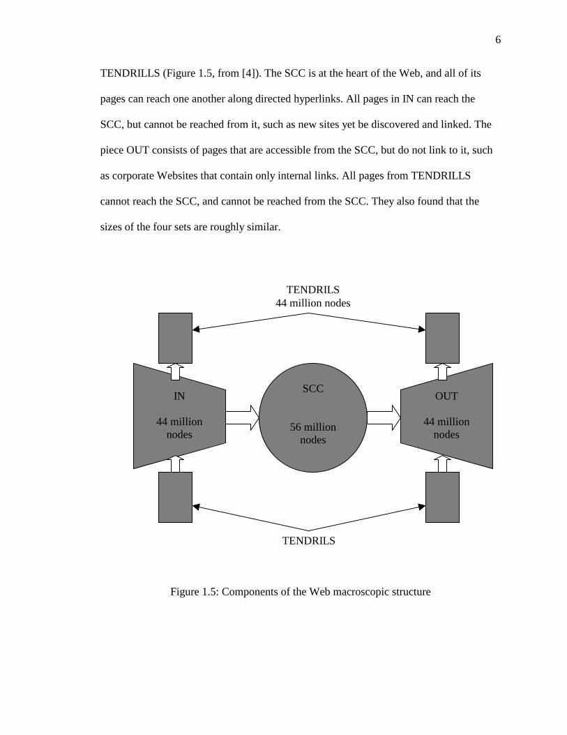
TENDRILLS (Figure 1.5, from [4]). The SCC is at the heart of the Web, and all of its

pages can reach one another along directed hyperlinks. All pages in IN can reach the

SCC, but cannot be reached from it, such as new sites yet be discovered and linked. The

piece OUT consists of pages that are accessible from the SCC, but do not link to it, such

as corporate Websites that contain only internal links. All pages from TENDRILLS

cannot reach the SCC, and cannot be reached from the SCC. They also found that the

sizes of the four sets are roughly similar.

Figure 1.5: Components of the Web macroscopic structure

OUT

44 million nodes

IN

44 million nodes

SCC

56 million nodes

TENDRILS

TENDRILS 44 million nodes

7

Picking random starting nodes for the BFS algorithm, Broder et al. [4] found that

BFS traversals exhibited a sharp bimodal behavior, i.e. it would either “die out” after

reaching a small set of nodes (90% of the time this set has fewer than 90 nodes; in

extreme cases it has a few hundred thousand), or it would "explode" to cover about half

of the total nodes in the graph. This interesting result may be related to degree

distributions, the Web’s macroscopic structure, and other Web properties, such as that the

distribution of sizes of SCCs also obeys a power law.

1.3 Crawling strategies

Understanding properties of the massive Web graph can help in designing

crawling strategies for the Web [5], in illuminating the sociology of content creation on

the Web [4], in analyzing the behavior of Web algorithms [3, 11], in predicting the

evolution of Web structure [12], and in predicting the emergence of new phenomena in

the Web graph. In this section, we will only focus on one application of the Web graph

structure: crawling.

A crawler is a program that retrieves Web pages, commonly used in a search

engine [6]. A crawler starts off with the URL for an initial page P0. It first retrieves P0,

extracts any URLs in it, and adds them to a queue of URLs to be scanned. Then the

crawler gets URLs from the queue, and repeats the process. Every page that is scanned is

given to a client that saves the pages, creates an index for the pages, or summarizes or

analyzes the content of the pages.

Because of the importance of crawlers on the Internet, crawlers are widely used

today. Major search engines such as Google [9], AltaVista [1], InfoSeek [10], Excite [8],

8

and Lycos [13] use crawlers to visit most text Web pages, in order to build content

indices. Crawlers may also be used to look only for certain types of information, such as

e-mail addresses.

The design of a good crawler presents many challenges. Externally, the crawler

must avoid overloading Web sites or network links as it goes about its business.

Internally, the crawler must deal with huge volumes of data [6]. Therefore, how to

carefully decide what URLs to scan and in what order remains an important question for

crawlers.

Cho, Garcia-Molina, and Page [6] suggested using connectivity-based document

quality metrics to direct a crawler towards high-quality pages. They performed a series of

crawls over 179,000 pages in the stanford.edu domain and used the following different

ordering metrics to direct the different crawls:

• Breadth-first ordering: pages are crawled in the order they are discovered;

• Backlink count ordering: pages with the highest number of known links to them

are crawled first;

• PageRank ordering: pages with the highest PageRank are crawled first;

• Random ordering: random pages from the set of uncrawled pages are selected

and crawled.

PageRank is the connectivity-based page quality measure suggested by Brin and

Page [3]. It is designed to rank pages in the absence of any queries, i.e. PageRank

computes the “global worth” of each page. Intuitively, the PageRank measure of a page is

similar to its in-degree, which is a possible measure of the importance of a page. The

PageRank of a page is high if many pages with a high PageRank contain links to it, and a

9

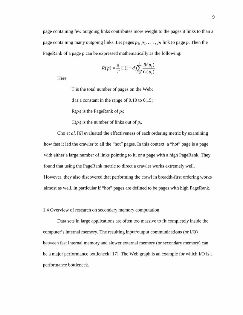
page containing few outgoing links contributes more weight to the pages it links to than a

page containing many outgoing links. Let pages p1, p2, . . . , pk link to page p. Then the

PageRank of a page p can be expressed mathematically as the following:

�=

−+=k

i i

i

pC

pRd

T

dpR

1 )(

)()1()( .

Here

T is the total number of pages on the Web;

d is a constant in the range of 0.10 to 0.15;

R(pi) is the PageRank of pi;

C(pi) is the number of links out of pi.

Cho et al. [6] evaluated the effectiveness of each ordering metric by examining

how fast it led the crawler to all the “hot” pages. In this context, a “hot” page is a page

with either a large number of links pointing to it, or a page with a high PageRank. They

found that using the PageRank metric to direct a crawler works extremely well.

However, they also discovered that performing the crawl in breadth-first ordering works

almost as well, in particular if “hot” pages are defined to be pages with high PageRank.

1.4 Overview of research on secondary memory computation

Data sets in large applications are often too massive to fit completely inside the

computer’s internal memory. The resulting input/output communications (or I/O)

between fast internal memory and slower external memory (or secondary memory) can

be a major performance bottleneck [17]. The Web graph is an example for which I/O is a

performance bottleneck.

10

Vitter and Shriver [18] introduced the secondary memory model as shown in

Figure 1.6. In that model, a machine consists of a CPU and a fast, internal memory of

size M, and D independent disks drives. The D disks are connected to the machine, so

that it is possible to transfer D*B items in one I/O. The model assumes that disk blocks

are indivisible and that is only possible to perform a computation on data that resides in

internal memory. This has become the standard complexity model for secondary memory

computation. Algorithmic performance is measured by counting the number of I/O

Figure 1.6: The secondary memory model of Vitter and Shriver

Disk 1

Disk D

Disk 2

Block Size B

……

Memory

M

CPU

11

operations executed, the number of CPU operations performed (RAM model), and the

number of occupied disk blocks. Assuming N is the size of the data, and B is the block

size, then important lower bounds for this model include the following:

• Scanning a set of N items: O(N/(DB)) I/Os;

• Sorting a set of N items: O(N/DB logM/B(N/B)) I/Os;

• Sorting a set of N items with k distinct keys, k < N: O(N/DB logM/BK)

I/Os;

• Online search among N items: O(logDBN) I/Os.

Based on the secondary memory model of Vitter and Shriver, there are currently

two systems that provide secondary memory computation in a general and flexible

manner. One is TPIE [16] (Transparent Parallel I/O Environment) from Duke University,

a C++ library that provides external programming paradigms such as scanning, sorting

and merging sets of items. TPIE realizes secondary memory by using several files on

disk. In fact, each data structure or algorithm uses its own file. Several different file

access methods are implemented. TPIE only offers some more advanced secondary

memory data structures and most of them are based on the external program paradigms

[2]. Direct access to single disk blocks is possible but complicated. TPIE offers no

connection to an efficient internal-memory library that is necessary when implementing

secondary memory algorithms and data structures.

Another library is LEDA-SM (LEDA for secondary memory) from Germany, a

C++ library that extends the internal-memory library LEDA (Library of Efficient Data

types and Algorithms) [7]. It offers the possibility of using advanced and efficient

12

internal memory data structures and algorithms in secondary memory algorithmic design.

Unlike TPIE, a collection of external memory data structures, including ext_stack,

ext_queue, ext_array, ext_graph, ext_r_heap, buffer-tree, B-tree, ext_matrix, are

provided in LEDA-SM. Simple algorithms, such as depth-first search and topological

sorting are also supported in LEDA-SM. Detailed information on LEDA-SM will be

introduced in Chapter 2.

1.5 The goal of the research

Recent research work [6, 14] has shown that breadth-first search crawling yields

high quality pages. Najork and Wiener [14] found that breadth-first search downloads hot

pages first, and the average quality of the pages decreases over the duration of the crawl.

However, very little has been done on increasing the overall download rate when using

breadth-first search crawling. This is not only necessary when crawlers are run on current

workstations with limited internal memory, but is also necessary for data servers with

large internal memories, since the number of Web pages has been increasing dramatically

in recent years.

The ultimate goal of our research is to enhance breadth-first search crawling, i.e.

studying how to reduce breadth-first search time for crawling. One option is to construct

highly compressed representations of Web graphs that can be stored and analyzed in

current machines with moderate amounts of main memory [15]. The alternative is to

compute massive graphs with I/O efficient techniques [17], i.e., applying efficient

secondary memory algorithms to process the Web graph. While the first option is

attractive because of computation speed in main memory, it may not be possible to fit

13

massive data sets in main memory in current machine even if they are compressed.

Accordingly, we selected the second method to study how to enhance BFS crawling.

In Section 1.4, we introduced two systems for efficient secondary memory

computation, TPIE and LEDA-SM. After comparing then, LEDA-SM library was

selected for our studying efficient computation of the WWW graph since LEDA-SM

contains external graph data structures and general algorithms, and the ability to support

these with efficient internal memory algorithms.

For our research, instead of using real data from the Web graph for the

experiments, we simulate the Web graph using node numbers but capturing important

Web properties. Real data sets will hopefully be the subject of future research on Web

graph computations.

14

CHAPTER 2

LEDA-SM

2.1 Architecture of LEDA-SM

LEDA-SM is implemented in C++. The library is divided into two layers, a kernel

layer and an application layer (Figure 2.1). The kernel layer is responsible for disk space

management and disk access. It is subdivided into the abstract kernel and the concrete

kernel. The concrete kernel is responsible for performing I/O, managing used and non-

used disk blocks, and managing users of disk blocks. The concrete kernel will be

introduced in Section 2.2.2 in much more detail. The abstract kernel implements a user-

friendly access interface to the concrete kernel (detailed information will be introduced in

Section 2.2.1). The application layer consists of a collection of secondary memory data

structures (e.g. ext_array, ext_queue, ext_graph) and algorithms (e.g. DFS, BFS). The

implementations of all applications use the classes of the abstract kernel to simplify

access to secondary memory. LEDA is used to implement the in-core part of the

secondary memory data structures and algorithms and the kernel data structures of

LEDA-SM. Secondary memory is implemented in LEDA-SM by using the file system of

the host operating system. Access to secondary memory is provided by file access

utilities of the operating system.

15

Figure 2.1 Architecture of LEDA-SM

2.2 The kernel structure of LEDA-SM

As mentioned above, the kernel of LEDA-SM is subdivided into a concrete kernel

and an abstract kernel. The concrete kernel consists of four classes: name_server,

ext_memory_manager, ext_disk and ext_freelist (see Figure 2.2). Class name_server

generates user identifiers, while ext_memory_manager implements disks and disk block

management. Both classes have only one instance. Class ext_memory_manager uses class

ext_disk to manage the disks and the access to disk blocks, and uses class ext_freelist to

manage the used and free blocks of a disk.

The abstract kernel provides the logical entities disk block identifiers (B_ID) and

blocks (block<E>). These entities are associated with their physical counterparts in the

concrete kernel as shown in Figure 2.2. Logical block identifiers are used to specify a

disk block on a specific disk. Class block is used to provide a templated type view (with

Concrete Kernel Layer

Kernel Layer

Abstract Kernel Layer

Application Layer

16

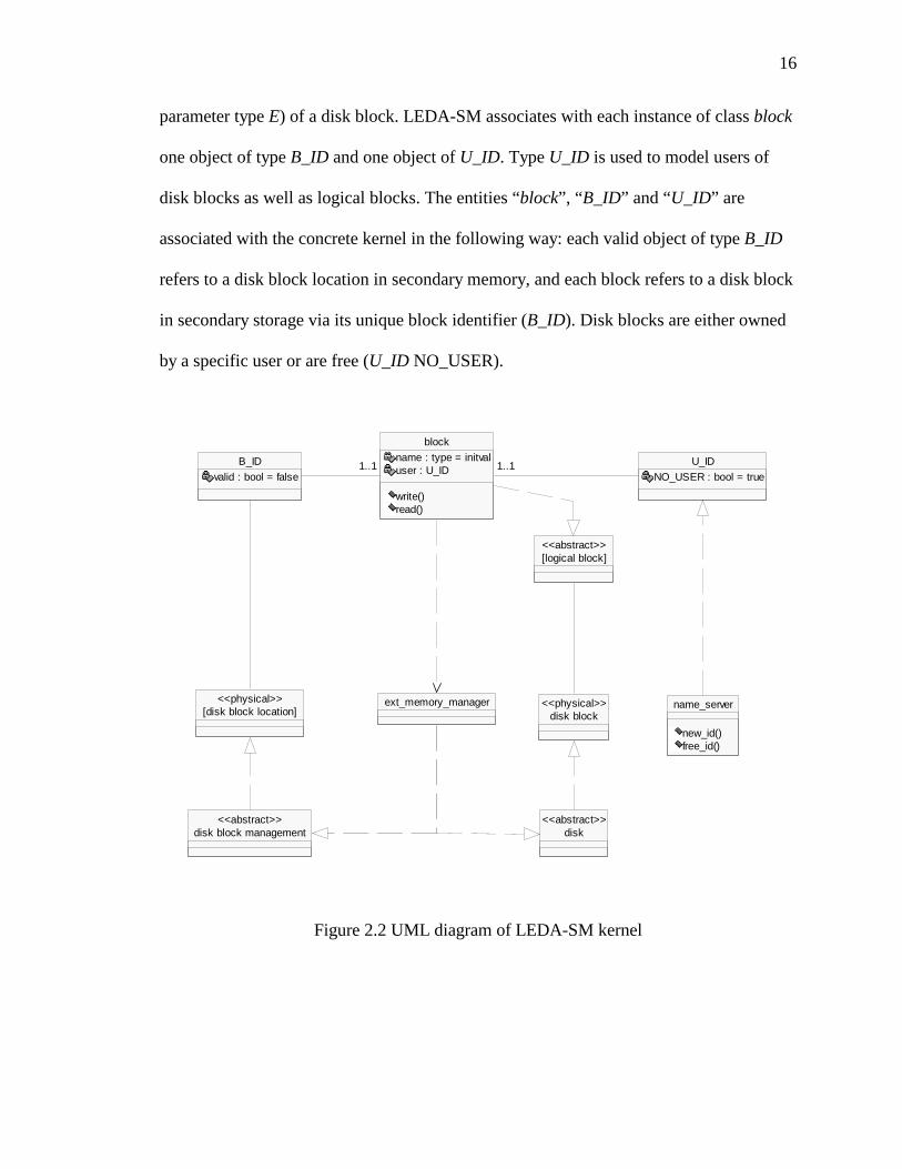
parameter type E) of a disk block. LEDA-SM associates with each instance of class block

one object of type B_ID and one object of U_ID. Type U_ID is used to model users of

disk blocks as well as logical blocks. The entities “block” , “B_ID” and “U_ID” are

associated with the concrete kernel in the following way: each valid object of type B_ID

refers to a disk block location in secondary memory, and each block refers to a disk block

in secondary storage via its unique block identifier (B_ID). Disk blocks are either owned

by a specific user or are free (U_ID NO_USER).

name_server

new_id()free_id()

ext_memory_manager

disk<<abstract>>

U_ID

NO_USER : bool = true

block

name : type = initvaluser : U_ID

write()read()

1..1

[disk block location]<<physical>>

B_ID

valid : bool = false1..1

disk block management<<abstract>>

disk block<<physical>>

[logical block]<<abstract>>

1..1 1..1

Figure 2.2 UML diagram of LEDA-SM kernel

17

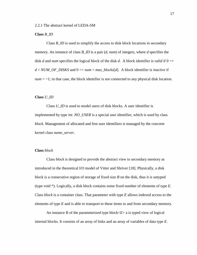
2.2.1 The abstract kernel of LEDA-SM

Class B_ID

Class B_ID is used to simplify the access to disk block locations in secondary

memory. An instance of class B_ID is a pair (d, num) of integers, where d specifies the

disk d and num specifies the logical block of the disk d. A block identifier is valid if 0 <=

d < NUM_OF_DISKS and 0 <= num < max_blocks[d]. A block identifier is inactive if

num = −1; in that case, the block identifier is not connected to any physical disk location.

Class U_ID

Class U_ID is used to model users of disk blocks. A user identifier is

implemented by type int. NO_USER is a special user identifier, which is used by class

block. Management of allocated and free user identifiers is managed by the concrete

kernel class name_server.

Class block

Class block is designed to provide the abstract view to secondary memory as

introduced in the theoretical I/O model of Vitter and Shriver [18]. Physically, a disk

block is a consecutive region of storage of fixed size B on the disk, thus it is untyped

(type void * ). Logically, a disk block contains some fixed number of elements of type E.

Class block is a container class. That parameter with type E allows indexed access to the

elements of type E and is able to transport to these items to and from secondary memory.

An instance B of the parameterized type block<E> a is typed view of logical

internal blocks. It consists of an array of links and an array of variables of data type E.

18

The array of links stores links to other blocks. A link is an object of data type B_ID

(block identifier). The second array stores variables of data type E. The number of

variables of the second array is calculated at the time of construction as follows:

blk_sz = (BLK_SZ - num_of_bids * sizeof(B_ID)) / sizeof(E)

where:

BLK_SZ is a system constant;

num_of_bids – the number of links.

There are two constructor types of class block:

block <E> B ; (1)

block<E> B(U_ID uid, int bids = 0). (2)

Constructor (1) creates an instance B of type block and initializes the number of links to

zero. At the time of creation, the block identifier is invalid, meaning that the block isn’ t

associated with a physical location in external memory. The internal user identification is

set to NO_USER. Constructor (2) creates an instance B of type block and initializes the

number of links num_of_bids and the user identifier uid. The block identifier is invalid as

in (1) at the time of creation. During write access to external memory, either a new

unused block identifier is requested from the external memory manager, or a disk block

specified by bid is set to the block identifier of B if the block identifier is inactive.

2.2.2 The concrete kernel of LEDA-SM

The concrete kernel is responsible for performing I/Os and managing disk space

and users in secondary memory. It consists of the four classes name_server,

19

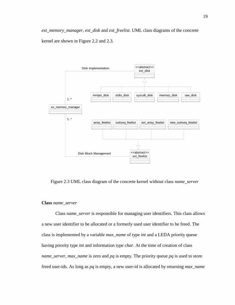
ext_memory_manager, ext_disk and ext_freelist. UML class diagrams of the concrete

kernel are shown in Figure 2.2 and 2.3.

1..*stdio_disk syscall_disk memory_disk raw_disk

array_freelist sortseq_freelist ext_array_freelist new_sortseq_freelist

mmpio_disk

ext_freelist<<abstract>>

ex_memory_manager

1..*1..*

Disk Block Management

ext_disk<<abstract>>Disk Implementation

1..*

Figure 2.3 UML class diagram of the concrete kernel without class name_server

Class name_server

Class name_server is responsible for managing user identifiers. This class allows

a new user identifier to be allocated or a formerly used user identifier to be freed. The

class is implemented by a variable max_name of type int and a LEDA priority queue

having priority type int and information type char. At the time of creation of class

name_server, max_name is zero and pq is empty. The priority queue pq is used to store

freed user-ids. As long as pq is empty, a new user-id is allocated by returning max_name

20

and increasing it. If pq is not empty, it returns its minimal key as the newly allocated

user-id.

Class ext_memory_manager

This class has only one instance at a time. The unique instance of this class is

created when the system starts up. It is mainly responsible for the following four tasks:

• kernel configuration

At the time of creation, the constructor will check if a system

configuration file named .config_leda-sm is located in the current working

directory. The file specifies the number of disks, name of the disk files,

size of the disk files, I/O implementation, and free list implementation (see

Table 2.1). If the configuration file exists, it will parse the configuration

file, and a configuration check is executed. Depending on circumstances,

the check may fail due to file creation error or disk device access error, or

if the requested disk space is not available.

• creation of secondary storage

After parsing the configuration file, ext_memory_manager uses

class ext_disk to create the secondary memory, i.e., it opens the files or

devices and sets up the disk block management.

• management of occupied and free disk blocks

At startup time, all disk blocks on each disk are free, i.e., they

don’ t belong to any user. It is possible to allocate blocks for a specific user

21

and free blocks. The requests are passed on to class ext_freelist, which is

responsible for the actual management of disk blocks on each disk.

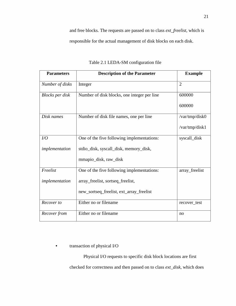
Table 2.1 LEDA-SM configuration file

Parameters Description of the Parameter Example

Number of disks Integer 2

Blocks per disk Number of disk blocks, one integer per line 600000

600000

Disk names Number of disk file names, one per line /var/tmp/disk0

/var/tmp/disk1

I/O

implementation

One of the five following implementations:

stdio_disk, syscall_disk, memory_disk,

mmapio_disk, raw_disk

syscall_disk

Freelist

implementation

One of the five following implementations:

array_freelist, sortseq_freelist,

new_sortseq_freelist, ext_array_freelist

array_freelist

Recover to Either no or filename recover_test

Recover from Either no or filename no

• transaction of physical I/O

Physical I/O requests to specific disk block locations are first

checked for correctness and then passed on to class ext_disk, which does

22

the actual physical I/O. The correctness check includes out-of-bounds

checks for the block identifiers as well as user checks.

Class ext_disk

Class ext_disk implements the logical disk drive and the access to it. It is a virtual

base class, i.e., it only describes the functionality while the actual implementations are

encapsulated in the classes memory_disk, stdio_disk, syscall_disk, mmapio_disk, aio_disk

and raw_disk. The actual implementation is chosen at the creation time of class

ext_memory_manager. Detailed information on derived classes will not be given here.

Member functions of class ext_disk are shown below.

Class ext_disk

{

public:

virtual void open_disk(int num) = 0;

virtual void close_disk( ) = 0;

virtual int write_blocks(int block_num, ext_block B, int k = 1) = 0;

virtual int read_blocks(int block_num, ext_block B, int k = 1) = 0;

virtual int read_ahead_blocks(int block_num, int ahead_num, ext_block

B) = 0;

virtual char* get_disktype( ) = 0;

} ;

23

Method open_disk(num) is used to create the disk space for logical disk num

(0 ≤ num < NUM_OF_BLOCKS). Information such as the file name of the disk and the

number of blocks on the disk is used by the external memory manager. Method

close_disk is used to disconnect the disks from the system. The actual physical I/Os are

implemented by read_blocks( ) and write_blocks( ). Method Read_ahead_block( ) is used

to read a single disk block and starts an asynchronous read-ahead of a second disk block.

Class ext_freelist

Class ext_freelist is responsible for managing free and allocated disk blocks. Class

ext_freelist is implemented as a virtual base class from which the actual implementation

classes are derived (see Figure 2.2). The classes include: array_freelist, sortseq_freelist,

ext_array_freelist and new_sortseq_freelist. The actual implementation is chosen at the

creation time of class ext_memory_manager. Detailed information on derived classes will

not be given here. Member functions of class ext_freelist are shown below.

Class ext_freelist

{

public:

virtual void init_freelist(int num) = 0;

virtual int new_blocks(U_ID uid, int k=1)=0;

virtual int free_blocks(int block_num, U_ID uid, int k = 1)=0;

virtual void free_all_blocks(U_ID uid)=0;

virtual bool check_owner(int block_num, U_ID uid, int k=1)=0;

24

virtual int get_blocks_on_disk( )=0;

virtual int get_free_blocks( )=0;

virtual int get_cons_free_blocks( )=0;

virtual int get_used_blocks( )=0;

virtual char* get_freelist_type( )=0;

virtual int size()=0;

} ;

Method init_freelist(num) is used to initialize the freelist for disk num,

0 ≤ num < NUM_OF_DISKS. Method new_blocks( ) is used to allocate k consecutive

blocks. The return value is the block number of the first allocated block on disk num.

Method free_blocks( ) returns previously allocated disk blocks of disk num back to the

freellist, while free_all_blocks( ) frees all disk blocks of disk num that are allocated to

user uid. Method check_owner( ) checks if k consecutive blocks starting at block

block_num are owned by user uid. Other methods are used to get free blocks, used blocks

and free list information.

2.3 External graph data structures and BFS

2.3.1 External array (ext_array)

The external array is introduced because of its extensive use by other external data

structures and algorithms. An instance A of the parameterized data type ext_array<E> is

a mapping from an interval I = [a..b] of integers, the index set of A, to the set of variables

of data type E, the element type of A. An external array uses a buffer area of bfs (the

25

number of buffer groups reserved for keeping data in main memory) in groups of bpb

(the number of blocks per buffer group) internal blocks. A paging algorithm controls this

buffer area, which is responsible for exchanging blocks between the buffer area and the

external memory. If paging is necessary, the pager always fetches or writes to a group of

bpb blocks. There are three predefined paging algorithms, namely Least Recently Used

(LRU), RANDOM and dummy_pager. The parameters bfs and bpb and the paging

algorithm implementation are chosen at creation time.

2.3.2 External graph

An instance G = (V, E) of the data type ext_graph<EXT_GRAPH_TEMPLATE> (or

EXT_GRAPH) defines an external graph, consisting of nodes V and a set of edges

E ⊆ V × V. The size of the set of nodes is denoted by |V|, and similarly |E| denotes the size

of the set of edges. Let e = (u, v) be an edge of G; u is called the source node of e, and v

is called the target node of e. Node u and v are also endpoints of e. All edges having

source node u are said to be adjacent from u. The external graph data type uses an

adjacency list representation, and the implementation is based on external arrays.

Nodes and edges also called the items of the external graph. The set of nodes is

indexed by a set of node indices of the data type ext_node<EXT_GRAPH> (or

EXT_NODE), and the set of edges by a set of edge indices of the data type

ext_edge<EXT_GRAPH> (or EXT_EDGE).

An external graph can be implemented as a parameterized graph. For each item,

two kinds of extra information can be stored with it. The first one is called fixed, since it

cannot be changed; the other is called variable and can be changed. These are called

26

fix_vtype and var_vtype for the nodes, and fix_etype and var_etype for the edges. The

fixed information represents some predefined data of the external graph, while the

variable information can be used for temporary information produced by the algorithm.

Each item is stored together with its two pieces of information in a container kept by the

external graph, which is of type called node_container<EXT_GRAPH>

(NODE_CONTAINER) or edge_container<EXT_GRAPH> (EDGE_CONTAINER).

Each instance of node_container stores four groups of information: a unique node

index number of data type ext_node, a label indicating whether the contained node is

marked, the core node information which is the list of edges (of the data type ext_edge)

going out of the node, and two extra pieces of information related to the node, the fixed

information and variable information. The layout of a node_container object is shown in

Figure 2.4.

node index label core node info. fixed info. variable info.

Figure 2.4: data layout of node_container

Each instance of edge_container also stores four groups of information: a unique

edge index number of data type ext_edge, a label indicating whether the contained edge is

marked, the core edge information which is the source and the target node of the edge

(both of the data type ext_node), and two extra pieces of information related to the edge:

the fixed information and variable information. The layout of an edge_container is shown

in Figure 2.5.

27

edge index label core edge info. fixed info. variable info.

Figure 2.5: data layout of edge_container

All data for an external graph instance are kept in external memory. More exactly,

two instances of the data type ext_array are used, one for the node containers, and the

other for the edge containers. Let G be an instance of the data type EXT_GRAPH, n be

the number of nodes of G, and m the number of edges of G. Then the space required in

external memory is O(n + m).

2.3.3 External Breadth First Search (BFS)

In external memory, graph algorithms can be classified as being either fully-external or

semi-external. Fully-external graph algorithms assume that amounts of information of

size Θ(|V|) or Θ(|E|) can not be stored in internal memory, while semi-external graph

algorithms are able to store such amounts of information of in internal memory. These

two types of BFS algorithm are supported in LEDA-SM by the following:

void EXT_BFS (T& G, NODE_ARRAY & A, EXT_NODE s, int dic_size = 8)

void EXT_BFS_int (T& G, NODE_ARRAY & A, EXT_NODE s)

Procedure EXT_BFS is the fully-external algorithm. It takes as arguments an external

graph G, an EXT_NODE s and a NODE_ARRAY A. It performs a breadth first search in

phases, starting at s, computing for every visited node w the distance DIST[w] from s to

w. On return the NODE_ARRAY A contains all nodes reached from s. The algorithm has

28

I/O complexity O ( ||*

||*||V

BS

EV + ), where S is the number of recursive calls during the

run, and B is the number of edges in one block.

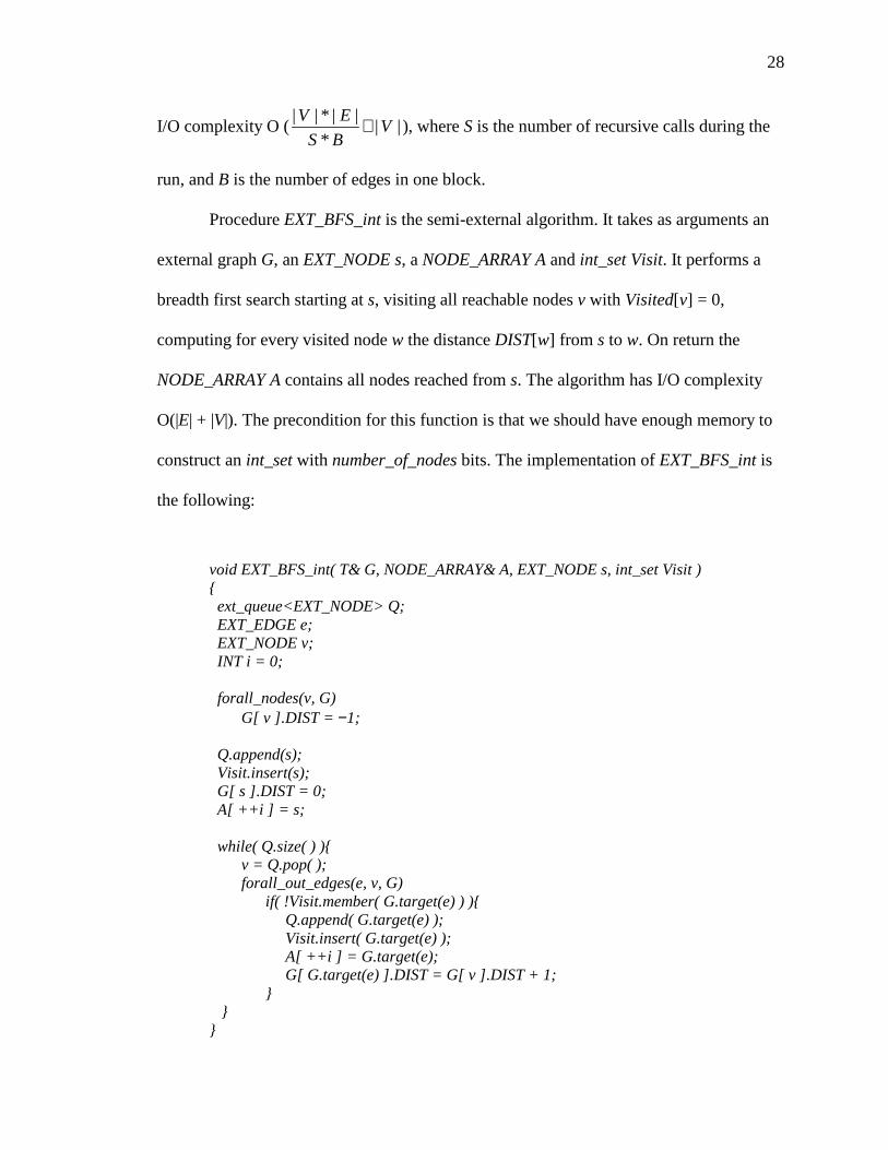
Procedure EXT_BFS_int is the semi-external algorithm. It takes as arguments an

external graph G, an EXT_NODE s, a NODE_ARRAY A and int_set Visit. It performs a

breadth first search starting at s, visiting all reachable nodes v with Visited[v] = 0,

computing for every visited node w the distance DIST[w] from s to w. On return the

NODE_ARRAY A contains all nodes reached from s. The algorithm has I/O complexity

O(|E| + |V|). The precondition for this function is that we should have enough memory to

construct an int_set with number_of_nodes bits. The implementation of EXT_BFS_int is

the following:

void EXT_BFS_int( T& G, NODE_ARRAY& A, EXT_NODE s, int_set Visit ) { ext_queue<EXT_NODE> Q; EXT_EDGE e; EXT_NODE v; INT i = 0; forall_nodes(v, G) G[ v ] .DIST = −1; Q.append(s); Visit.insert(s); G[ s ] .DIST = 0; A[ ++i ] = s; while( Q.size( ) ){ v = Q.pop( ); forall_out_edges(e, v, G) if( !Visit.member( G.target(e) ) ){ Q.append( G.target(e) ); Visit.insert( G.target(e) ); A[ ++i ] = G.target(e); G[ G.target(e) ] .DIST = G[ v ] .DIST + 1; } } }

29

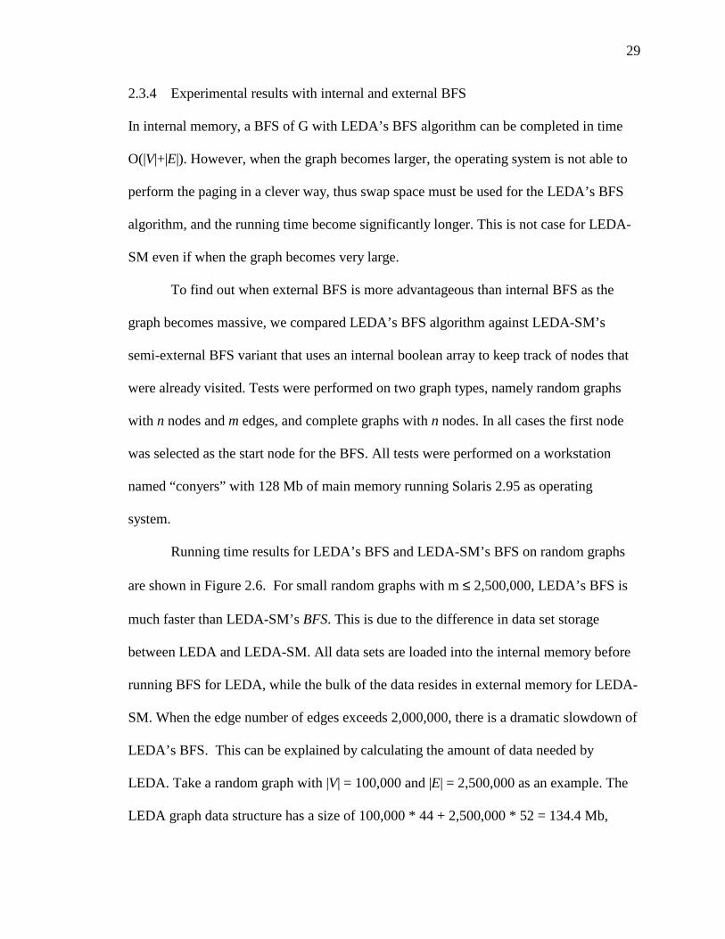
2.3.4 Experimental results with internal and external BFS

In internal memory, a BFS of G with LEDA’s BFS algorithm can be completed in time

O(|V|+|E|). However, when the graph becomes larger, the operating system is not able to

perform the paging in a clever way, thus swap space must be used for the LEDA’s BFS

algorithm, and the running time become significantly longer. This is not case for LEDA-

SM even if when the graph becomes very large.

To find out when external BFS is more advantageous than internal BFS as the

graph becomes massive, we compared LEDA’s BFS algorithm against LEDA-SM’s

semi-external BFS variant that uses an internal boolean array to keep track of nodes that

were already visited. Tests were performed on two graph types, namely random graphs

with n nodes and m edges, and complete graphs with n nodes. In all cases the first node

was selected as the start node for the BFS. All tests were performed on a workstation

named “conyers” with 128 Mb of main memory running Solaris 2.95 as operating

system.

Running time results for LEDA’s BFS and LEDA-SM’s BFS on random graphs

are shown in Figure 2.6. For small random graphs with m ≤ 2,500,000, LEDA’s BFS is

much faster than LEDA-SM’s BFS. This is due to the difference in data set storage

between LEDA and LEDA-SM. All data sets are loaded into the internal memory before

running BFS for LEDA, while the bulk of the data resides in external memory for LEDA-

SM. When the edge number of edges exceeds 2,000,000, there is a dramatic slowdown of

LEDA’s BFS. This can be explained by calculating the amount of data needed by

LEDA. Take a random graph with |V| = 100,000 and |E| = 2,500,000 as an example. The

LEDA graph data structure has a size of 100,000 * 44 + 2,500,000 * 52 = 134.4 Mb,

30

while the machine running LEDA BFS has 128 Mb of RAM. Therefore, swap space must

be used for this massive graph. The paging algorithm of the operating system is not able

to exploit locality of reference, although the LEDA graph data structure (adjacency lists)

does exhibit locality of reference for BFS.

0

200

400

600

800

1000

1200

1000

000

1500

000

2000

000

2500

000

3000

000

3500

000

4000

000

4500

000

5000

000

Edges

Ru

nn

ing

Tim

e (s

ec)

LEDA

LEDA-SM

Figure 2.6: Comparison of LEDA BFS and LEDA-SM BFS with an internal bit array on random graphs with 100,000 nodes and m edges

Comparison of results from LEDA’s BFS and LEDA-SM’s BFS on complete

graphs with n nodes are shown in Figure 2.7. From the results of complete graphs, we

find the advantage of LEDA-SM over LEDA is more obvious, compared with the results

from random graphs. A possible reason could be the different properties which hold for

random graph and complete graphs. In the case of random graphs, we can’ t guarantee

that the increase in the size of the part of the graph G which is reachable from the first

31

node is in proportion to the increase in the number of nodes |V| and edges |E|, although

some relationship between them exists. For complete graphs, the entire graph G is

reachable from any node, so this exactly reflects the increase in the numbers of nodes and

edges. Therefore, the results for complete graphs reflect the difference between LEDA

and LEDA-SM more quickly than those for random graphs.

0

50

100

150

200

250

300

350

1000 1200 1400 1600 1800 2000 2200 2400

Nodes

Run

ning

Tim

e

LEDA

LEDA-SM

Figure 2.7: Comparison of LEDA BFS and LEDA-SM BFS with an internal bit array on complete graphs with n nodes

32

CHAPTER 3

SIMULATION OF THE WEB GRAPH

3.1 Generating a model of the Web graph

The Web graph has a number of distinctive properties, as described in Section 1.2. In this

section, we will introduce models of the Web graph. Roughly speaking, we try to capture

the most important properties of the real world Web graph, i.e., degree distribution and

Web macroscopic features. The distributions of in-degrees and out-degrees of the Web

graph follow power laws. The exponent of the power law for in-degrees is consistently

around 2.1, while the exponent for out-degrees is 2.72 [4].

3.1.1 Simulating the Web graph’s degree distribution properties

3.1.1.1 Determining parameters for in-degrees and out-degrees

Broder et al. [4] found that the distribution of in-degrees follows a power law with

exponent 2.1. They also found that the node probability is a little bit higher than that

given by the power law when the degree exceeds 120. Based on these facts, the following

relationships should hold approximately:

1.2121

120

11.2

1||

1||||

iV

iVV

k

ii��==

×××+××= δαδ ; (1)

1.2121

120

11.2

1||

1||||

iVi

iViE

k

ii��==

××××+×××= δαδ . (2)

Here

33

|V| is the number of nodes of the Web graph;

|E| is the number of edges of the Web graph;

i is the in-degree;

δ is the proportion of nodes with in-degree 1;

k is the largest possible in-degree;

α is a positive constant.

Let ρ = ||

||

E

V; then equations (1) and (2) can be reformulated as follows:

��==

××+×=k

ii ii 1211.2

120

11.2

111 αδδ ; (3)

1.2121

120

11.2

11

ii

ii

k

ii��==

×××+××= αδδρ . (4)

Now given ρ, α (a positive constant) and δ (the proportion of nodes with in-

degree 1) can be determined based on equations (3) and (4).

Similarly, the distribution of out-degrees follows the power law with exponent

2.72 [4]. The node probability is a little bit higher than that given by the power law when

the degree exceeds 100. Based on these facts, the following relationships should hold

approximately:

72.2

k

101

100

172.2

1||

1||||

iV

iVV

ii��

′

==

×××+××= γβγ ; (5)

+×××=�=

100

172.2

1||||

i iViE γ

72.2

k

101

1||

iVi

i�

′

=

×××× γβ . (6)

Here

|V| is the number of nodes of the Web graph;

|E| is the number of edges of the Web graph;

34

i is the out-degree;

γ is the proportion of nodes with out-degree 1;

k′ is largest possible out-degree;

β is a positive constant.

Let ρ = ||

||

E

V; then equations (5) and (6) can be reformulated as follows:

��′

==

××+×=k

10172.2

100

172.2

111

ii iiβγγ ; (7)

72.2

k

101

100

172.2

11

ii

ii

ii��

′

==

×××+××= βγγρ . (8)

Now given ρ, β (a positive constant) and γ (the proportion of nodes with out-

degree 1) can be determined based on equations (7) and (8).

3.1.1.2 Constructing the source node array

We now know from Section 3.1.1.1 that parameters for the out-degrees can be

determined given n = |V| and m = |E|, and are now ready to construct the source node

array Source. This will be an external array of type ext_array. Let a = ��

���

� ××72.21

1nγ ,

b = a + ��

���

� ××72.22

1nγ , etc. The array Source can be filled in as follows: nodes 1, 2, 3

…… a each appear once, representing the nodes with out-degree 1, and they are filled in

the array as Source[0], Source[1], Source[2] …… Source[a-1]; nodes a + 1, a + 2 …… b-

1, b each appear twice, representing the nodes with out-degree 2, an so on. The layout of

the source node array Source is shown in Figure 3.1.

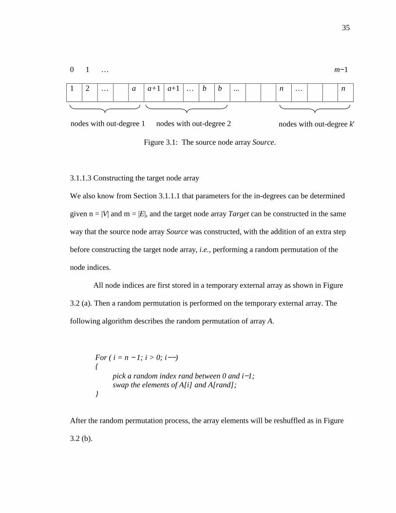
35

0 1 … m−1

1 2 … a a+1 a+1 … b b ... n … n

Figure 3.1: The source node array Source.

3.1.1.3 Constructing the target node array

We also know from Section 3.1.1.1 that parameters for the in-degrees can be determined

given n = |V| and m = |E|, and the target node array Target can be constructed in the same

way that the source node array Source was constructed, with the addition of an extra step

before constructing the target node array, i.e., performing a random permutation of the

node indices.

All node indices are first stored in a temporary external array as shown in Figure

3.2 (a). Then a random permutation is performed on the temporary external array. The

following algorithm describes the random permutation of array A.

For ( i = n − 1; i > 0; i−−) { pick a random index rand between 0 and i−1; swap the elements of A[ i] and A[ rand] ; }

After the random permutation process, the array elements will be reshuffled as in Figure

3.2 (b).

nodes with out-degree 1 nodes with out-degree 2 nodes with out-degree k′

36

(a)

0 1 2 … s−1 s … t−1 … n−1

1 2 3 … s s+1 … t … n

(b)

0 1 2 … s−1 s … t−1 … n−1

f g h … o p … q r

Figure 3.2: The temporary array A of type ext_array and length n.

(a) Node elements filled in the array starting from 1 to n in an ascending order.

(b) The reshuffled temporary array with node numbers randomly permuted.

Now we are ready to construct the target node array Target. This will be an

external array of type ext_array. Let s = ��

���

� ××1.21

1nδ , t = s + ��

���

� ××1.22

1nδ , etc. The

array Target can be filled in as follows: nodes f, g, h …… o each appear once,

representing the nodes with in-degree 1, and they are filled in the array as Target[0],

Target[1], Target[2] …… Target[s-1]; nodes p …… q each appear twice, representing

the nodes with out-degree 2, and so on. The layout of the target node array Target is

shown in Figure 3.3 (a).

3.1.1.4 Generating the edges

Edges can be obtained based on the existing source and target node arrays. A

random permutation on the target node array is performed before pairing source and

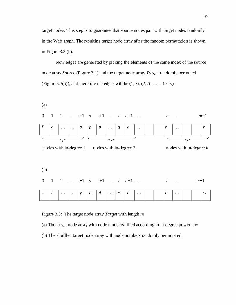
37

target nodes. This step is to guarantee that source nodes pair with target nodes randomly

in the Web graph. The resulting target node array after the random permutation is shown

in Figure 3.3 (b).

Now edges are generated by picking the elements of the same index of the source

node array Source (Figure 3.1) and the target node array Target randomly permuted

(Figure 3.3(b)), and therefore the edges will be (1, z), (2, l) ……. (n, w).

(a)

0 1 2 … s−1 s s+1 … u u+1 … v … m−1

f g … … o p p … q q ... r … r

(b)

0 1 2 … s−1 s s+1 … u u+1 … v … m−1

z l … … y c d … x e … h … w

Figure 3.3: The target node array Target with length m

(a) The target node array with node numbers filled according to in-degree power law;

(b) The shuffled target node array with node numbers randomly permutated.

nodes with in-degree 1 nodes with in-degree 2 nodes with in-degree k

38

3.1.2 Refining the Web graph simulation with the help of other properties

Based on the experiments on 200 million pages and 1.5 billion hyperlinks from Broder et

al. [4], we can compute the ratio of edges to nodes (also called ρ). This value was used in

our simulated Web graphs as described in Section 3.1.1. External BFS was then tested on

simulated Web graphs with 2 million nodes. In all cases, the last node of the simulated

Web graph was selected as the start node. The last node is the node with the largest out-

degree based on our model of the Web graph. In our tests, node 2,000,000 was the last

node. The execution times of BFS indicated that the number of nodes reachable from the

start node is small. This was confirmed by recording the number of nodes visited. This

means that the simulated Web graphs are composed of many small strong connected

components, even though their degree distributions follow realistic power laws. In

contrast, most of the real Web graph is contained in just four components. The possible

reason is that we underestimated the value of ρ when we simulated Web graphs with 2

million nodes. To accurately simulate the Web graph, we need to better estimate the

value of ρ and the constants α for in-degree nodes and β for out-degree nodes.

Broder et al. [4] found that BFS traversals exhibited sharp bimodal behavior, i.e.,

it either reaches a small set of nodes, or else covers about half of all the nodes of the Web

graph. Based on the fact that nodes of high out-degree should reach about half of total

nodes, we estimated the constant ρ as follows. Given a test value of ρ, we record the

number of nodes visited when running BFS. Initially, ρ was set to 7.5. The value of ρ

was increased until we found that the number of nodes visited was about half the total

number of nodes.

39

3.2 BFS on simulated Web graphs

Simulated Web graphs were generated as described in Section 3.1. We simulated Web

graphs with 2 million nodes and several values of ρ. Different values of ρ were used in

order to find a value of ρ accurately reflecting the real world Web graph. All tests were

run on a large Sun server (with 8 processors and 32Gb RAM) named “rna” . Table 3.1

shows some parameters for simulated Web graphs with the different values of ρ, and the

running time results of BFS on these graphs.

From Table 3.1, we see that the number of nodes visited is about half of the total

number when the value of ρ is around 19.5. Accordingly, we conclude that this value

gives the best model of the real world Web graph. The running time of BFS on this

simulated graph is 4694 seconds, or about 1.3 hours.

Table 3.1: Parameters of the simulated Web graphs and BFS results

ρ (The ratio of edges to nodes) 14.0 17.6 19.5 20.1

α (The constant for in-degree) 10.0 13.0 14.5 15.0

δ (The proportion of nodes

with in-degree 1)

0.6245 0.6192 0.6165 0.6156

β (The constant for out-degree) 375.4 490.8 549.9 569.8

γ (The proportion of nodes

with out-degree 1)

0.7428 0.7296 0.7231 0.7209

The number of nodes visited 69,005 76656 1,128,073 2,000,000

The running time of BFS (sec.) 288 319 4694 7797

40

CHAPTER 4

CONCLUSIONS AND FUTURE WORK

With the growth of the size of the WWW, efficient crawling for use by search engines

will become more and more important for satisfactory search results. Cho et al. [6]

showed that using a connectivity-based ordering metric (e.g., PageRank) could steer the

crawler towards higher-quality pages. However, computing PageRank values for several

hundred million or more pages is an extremely expensive computation. On the other

hand, crawling in breadth-first search order also yields high quality pages during the early

stages of the crawl, while not incurring such high computation costs. The reason breadth-

first search obtains high quality pages is that important pages have many links to them

from numerous hosts, and those links will be found early, regardless of which host or

page the crawl originates on [14]. Therefore, crawling in breadth-first search order is an

efficient and practical crawling technique in the real world.

We know the Web graph is a massive graph, and data sets for the Web graph are

too large to fit in any single computer’s internal memory. Therefore, running bread-first

search of the Web graph in the internal memory of most of our computers is impossible.

We used data structures provided by LEDA-SM to store huge data sets for our simulated

Web graphs. The simulated Web graphs share important properties with the real Web

graph, i.e., the degree distributions follow the same power laws, and random-start BFS

traversals exhibit sharply bimodal behavior. Due to limitations of the LEDA package,

41

only LEDA-SM BFS was tested on the simulated Web graphs. However, the results of

LEDA BFS and LEDA-SM BFS on random and complete graphs indicate that LEDA-

SM will perform better than LEDA on the simulated Web graphs. Thus, we believe that

the LEDA-SM system would be useful for Web graph computations, especially on

machines with modest amounts of main memory.

At present there is no version of LEDA that supports 64-bit code on Solaris, so

data sets of graphs cannot be larger than 4 Gb. This limits the size of graphs when doing

comparison tests of LEDA BFS and LEDA-SM BFS. We believe that the LEDA-SM will

show increased improvement over LEDA for more massive graphs once 64-bit code is

supported.

The real world Web graph is a very complicated graph with many special

properties. Our simulation of Web graphs captures some important properties of the Web

graph, such as degree distributions. For future research, additional features of the real

Web graph need to be accurately simulated. These include unevenness in the degree

distribution, and some amount of correlation between in-degrees and out-degrees. In

addition, our simulated Web graphs don’ t contain real information other than incidence

of nodes and edges. The additional information needed for real Web graphs could be

modeled in the simulations. Of course real data sets for the Web graph would be best for

testing BFS for crawling.

42

REFERENCES

[1] Alta vista Home Page, http://altavista.digital.com/.

[2] L. Arge, O. Procopiuc, J. S. Vitter. “ Implementing I/O-Efficient Data Structures

Using TPIE”. Proceedings of the 10th European Symposium on Algorithms (ESA

'02), Rome, Italy, 88-100, 2002.

[3] S. Brin, and L. Page. “The anatomy of a large scale hypertextual Web search

engine” . In Proceedings of the 7th International World Wide Web Conference,

107-117, 1998.

[4] A. Broder, R. Kumar, F. Maghoul, P. Raghavan, S. Rajagopalan, R. Stata, A.

Tomkins and J. Wiener. “Graph structure in the Web: experiments and models” .

Computer Networks, 33: 309-320, 2000.

[5] J. Cho and H. Garcia-Molina. “Synchronizing a database to improve freshness” .

In 2000 ACM International Conference on Management of Data (SIGMOD),

355-366, 2000.

[6] J. Cho, H. Garcia-Molina and L. Page. “Efficient crawling through URL

ordering” . In Proceedings of the 7th International World Wide Web Conference,

161-172, 1998.

43

[7] A. Crauser. LEDA-SM: External memory algorithms and data structures in theory

and practice. PhD thesis, Universität des Saarlandes, 2001.

[8] Excite Home Page, http://www.excite.com/.

[9] Google Home Page, http://www.google.com/.

[10] InfoSeek Home Page, http://www.infoseek.com/.

[11] J. Kleinberg. “Authoritative sources in a hyperlinked environment” , In

Proceedings the 9th ACM-SIAM Symposium on Discrete Algorithms, 668-677,

1998.

[12] R. Kumar, P. Raghavan, S. Rajagopalan, and A. Tomkins. “Trawling the Web for

cyber communities ” , Computer Networks, 31: 1481-1493, 1999.

[13] Lycos Home Page, http://www.lycos.com/.

[14] M. Najork and J. Wiener. “Breadth-first search crawling yields high-quality

pages” . In Proceedings of the 10th International World Wide Web Conference,

114-118, 2001.

[15] T. Suel and J. Yuan, “Compressing the graph structure of the Web”. In

Proceedings of the IEEE Data Compression Conference (DCC), 213-222, 2001.

[16] TPIE Home Page, http://www.cs.duke.edu/~tpie/.

44

[17] J.S. Vitter. “External algorithms and data structures: dealing with massive data” .

Computing Surveys, 33: 209-271, 2001.

[18] J.S. Vitter and E.A.M. Shriver. “Optimal algorithms for parallel memory I: two

level memories. Algorithmica, 12: 110-147, 1994.