application of electrostatic analogy …tf.llu.lv/conference/proceedings2017/papers/n331.pdf ·...

ENGINEERING FOR RURAL DEVELOPMENT Jelgava, 24.-26.05.2017.

1458

APPLICATION OF ELECTROSTATIC ANALOGY METHOD BASED ON DIFFERENTIAL

OHM’S LAW IN NDT SYSTEMS FOR MONITORING INTERNAL DEFECTS IN

PIPELINES MADE OF CONDUCTIVE MATERIALS IN AGRICULTURE

Bazhenov Anatoliy, Bondareva Galina, Grivennaya Natalia, Malygin Sergey

Don State Technical University, Russia

[email protected], [email protected],

[email protected], [email protected]

Abstract. The proposed method of estimating the conductive plate thickness allows carrying out the non-

destructive testing of the objects that are made of conductive materials when there is a possibility of electrical

contact with the surface of the object. In particular, the method allows assessing the current state of corrosion

changes of irrigation systems in agriculture. The method implies using the Ohm’s law in differential form.

Keywords: electrodynamics, Ohm’s law in differential form, monitoring, corrosion, pipelines.

Introduction

The considerable share of accidents on pipelines because of corrosion of pipes requires urgent

researches in the field of anticorrosive protection [1; 2] and creation of monitoring aids of corrosion of

pipelines [3-5], including irrigation systems in agriculture. The possibility to determine the critical

corrosion level and changes in a pipe on the basis of instrumental and analytical forecast allows not

only to provide well-timed replacement of pipeline sections but also to substantiate the use of

specialized electrical, chemical or mixed corrosion prevention methods.

All types of nondestructive testing, which are currently in use, can be divided into three main

groups: methods based on the interaction of electromagnetic fields and elementary particles with the

test objects; methods based on the use of acoustic fields; methods based on the interaction of

penetrating substances with the objects under control [6].

Electric NDT is based on recording the parameters of the electric field interacting with the object

under control or occurring in a controlled object as a result of external influence.

The method for assessing the conducting plate thickness put forth below allows measuring the

degree of integrity of any metal equipment or structure and also allows evaluating both

electrochemical and mechanical actions [7].

Materials and methods

Electrical resistance method (ER) is based on the differential Ohm’s law implementation and

implies the measurement of electrical resistance of the controlled object portion [8]. The measurement

is performed in the orthogonal planes, using the source of DC voltage. The method is used to measure

the product wall thickness with one-sided access, to measure the coating thickness, for detecting

defects in electrically conductive test objects [9; 10].

For plotting the lines of currents in a conducting medium caused by the external source of DC

voltage, we use the analytical expressions to determine the equipotential surfaces and electrostatic

field lines of two charged axes (Fig. 1) [8; 11].

The equation of the equipotential lines of two charged axes is the ratio

.1

2 constr

rk == (1)

This expression corresponds to the circumference

222=R )+(y-y )(x-x cc (2)

where xc, yc – circumference center coordinates;

R – radius of the circle.

Taking into account the agreed notations from Fig. 1 and expression (2) we obtain

DOI: 10.22616/ERDev2017.16.N331


1459

Fig. 1. Lines of force and equipotential lines

.1

2;0;

1

122

2

)-k(

ka± =R=y

)-k(

)+k(a±s==x cc (3)

The plus sign is taken for, k < 1 (r2 < r1 is the location of negatively charged axis), the minus sign

is taken for k > 1 (r2 < r1 is the location of positively charged axis).

Thus, as it follows from (1) and (2), the equipotential lines are circles with centers located on the

x-axis. Using (2), it is possible to draw an equipotential line on the plane (or equipotential surface

representing the circular cylinder in space). The y-axis, along which the potential is equal to zero,

reflects the equipotential plane in space; φ = 0 in each point of it (Fig. 1).

To build the force field lines it is necessary to use the relation E̅ = -gradφ, which implies that the

force and equipotential lines of the electrostatic field are mutually orthogonal. It should be

remembered that the source of the force lines are positive charges and the drain is negative. In this

case, the force field lines on the plane are a family of circumferences

,2222

cEcE y+=a )y-(y+(x) (4)

with the centers ycE on the y-axis and the radii RE, equal to the distance from their centers to the

charged axes (Fig. 1):

22,0cE

EcE y+aR=x = . (5)

For the simulation of equipotential surfaces and force field lines, we will use an integrated Matlab

package [12]. The resulting equipotential surfaces and force lines of the electrostatic field of two

charged axes has been shown in Fig. 2.

Fig. 2. Results of simulating equipotential surfaces (blue lines)

and force field lines (red lines)


1460

To determine the thickness d of the plate of the conductive material at the points A and B (Fig. 3),

we install the electrodes connected to the source of DC voltage.

Fig. 3. Arrangement of electrodes on the test plate

Equipotential surfaces and force field lines will be truncated spheres with the radii calculated by

the formulae (3) and (5), respectively (Fig. 4).

Fig. 4. Simulating of equipotential surfaces by the truncated spheres

The dependence of the radius of equipotential surfaces RE on the parameter k (1) is shown in

Fig. 5.

Fig. 5. Radius of the equipotential surfaces RE in relation to the k coefficient

Fig. 6 shows a graph of changes in the magnitude of the displacement of the center of the

equipotential surface xc along the x-axis.

Since s2 – a

2 = R

2, then at a = 2 the graphs presented in Fig. 5 and Fig. 6 practically coincide. As it

follows from the graphs, there are such values of initial data (in particular, the k parameter), at which

changes occur most intensively. This conclusion allows considering only a limited area of the initial

data when modeling and thereby reduces the computational load of the algorithm.


1461

Fig. 6. Displacement of the center of equipotential surface xc along the x-axis

Fig. 7 a, b present the simulated field lines on the surface of the conductor with different

increments of displacement from the sphere center.

а) b)

Fig. 7. Family of field lines on the surface of the object under test

For the two spheres, the centers of which are equidistant from the line connecting the electrodes,

the area of their intersection characterizes the surface of the conductor with the same density of

electric current (Fig. 8).

Fig. 8. Formation of the surface with identical current density

The surface area can be determined by the formula of the area of a spherical segment lateral

surface:

). +h(a= hR=M E222 ππ (6)

The meaning of the variables in the expression (6) is illustrated in Fig. 9.


1462

Fig. 9. Meaning of the variables in the expression (6)

Fig. 10 shows the dependency graph displaying how the area of the spherical segment M lateral

surface depends on the magnitude h of the displacement of the sphere edge from the centerline AB.

Fig. 10. Change of the area of the lateral surface of spherical segment M depending on the

magnitude of the radius displacement h

The analysis of Fig. 10 shows that for simulating it is sufficient to explore only, [–a; a] site, on

which changes of the graph occur most intensively.

Under constraints on the thickness of the test object, a part will be cut out of the lateral surface

area; this part is proportional to the difference a – d (Fig. 9).

To calculate the area of the cutout figure, it is necessary to evaluate the integral of the form

.)(

4222

) dy) dxyyxR

R(S(D)=

b

h-b cE

Ea

d

∫∫−−−

(7)

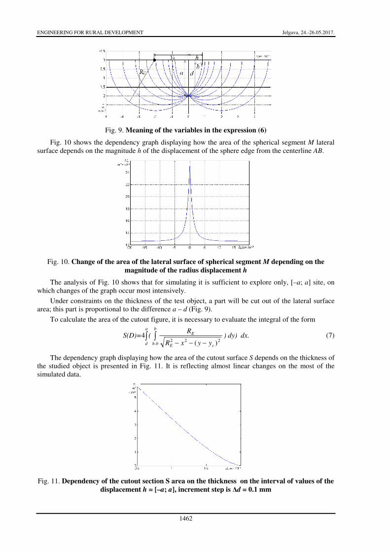
The dependency graph displaying how the area of the cutout surface S depends on the thickness of

the studied object is presented in Fig. 11. It is reflecting almost linear changes on the most of the

simulated data.

Fig. 11. Dependency of the cutout section S area on the thickness on the interval of values of the

displacement h = [–a; a], increment step is ∆d = 0.1 mm


1463

Fig. 12 shows a family of curves, reflecting the change in the area of the spherical segment lateral

surface taking into account the thickness of the object.

Fig. 12. Current density distribution over the d = 0.5:0.5:2 thickness; red line d = 2

The surface area of a spherical segment is proportional to the density of the electric current

flowing through the given line of force. Changing of the test object thickness results in the

corresponding change of the surface area and, consequently, the change in the current density, which

are reflected in the model.

From the contents of Fig. 12, it follows that the change in the thickness of the test object has a

significant influence on local densities of electric current; therefore, it is possible to measure the object

thickness and its change by measuring the electrical parameters associated with the local density of

electric current.

We will place electrodes in points A and B (Fig. 13) and connect them to the source of DC

voltage. Then we will measure the voltage at points C, D, 1, 2, 3, 4 and 5.

Fig. 13. Electrode arrangement diagram

According to the integral form of the Kirchhoff’s second law, there must be a logical connection

between the measured voltages.

The Kirchhoff’s second law in integral form relates the voltages on the sections of the loop and

EMFs acting in the chosen loop. The integral form of the Kirchhoff’s second law can be obtained by

integrating the generalized Ohm’s law (or Kirchhoff’s second law) in differential form (5) along a

closed loop taken in the area of action of external forces (Eext̅ ≠ 0).

Let us consider the loop consisting of the branches l1, l2, …, lk, …, ln, lk – (the part of the loop

along which the current density is equal to Jk). We can rewrite (5) as:


1464

.σ

J=E +E (12)

We will integrate (12) in a closed loop

.ldJ

=l dE +ldELL

ext

L

∫∫∫ σ

Taking into account the condition of the potentiality of the DC electric field, we get:

.ldJ

l dELL

ext ∫∫ =σ

(13)

It is known [8], that

ldEL

ext .ek

n

1=k∑∫ =

where ek – EMF acting on the lk part of the loop;

∑ =

n

k ke1

– algebraic sum of the EMFs acting in the chosen closed loop.

Taking into account the equality of lk and, respectively, Jk̅ , measured at points C and D, 1 and 3, 2

and 4, the voltages U(J) are pairwise equal. The inequality of voltages characterizes the presence of

local defects.

The voltages measured on one current line (for example, at points 1 and 2) are proportional to the

distance from the general output (the negative terminal). From the expression (13) and the measured

voltages U(J), local current densities are determined in different field lines (streamline surfaces). Next,

the plate thickness is determined using the dependencies of the local current density on the h shift (see

Fig. 9). The guidelines for using the graphs are shown in Fig. 14.

Fig. 14. Procedure for determining the thickness of the plate

Conclusions

The mathematical models obtained from the given above mathematical dependencies have

become the basis for the proposed method. They allow determining the thickness of the conductive

plate when electrodes are arranged at one side of the test object. Mathematical simulation confirms a

possibility to observe internal corrosion changes that are comparable to massive corrosion on the depth

of 0,1 mm, at the same time the output voltage changes by an amount 0,1 mV [13]. In this case, the

statistical measurement error must be minimal. To assess the accuracy of the method, it is necessary to

execute the statistical analysis similar to [14].

References

1. Brossia S.C. The use of probes for detecting corrosion in underground pipelines, Underground

Pipeline Corrosion. Woodhead Publishing. 2014. pp. 286-303.


1465

2. Popov B.N., Kumaraguru S.P. Cathodic protection of pipelines. Handbook of environmental

degradation of materials. Second Edition. Oxford: William Andrew Publishing, 2012. 910 p.

3. Glisic B. Sensing solutions for assessing and monitoring pipeline systems. Woodhead Publishing

Series in Electronic and Optical Materials. vol. 56. 2014. pp. 422-460.

4. Datta S., Sarkar S. A review on different pipeline fault detection methods. Journal of Loss

Prevention in the Process Industries, vol. 41. pp. 97-106.

5. Jiles D.C. Review of magnetic methods for nondestructive evaluation. NDT International. vol. 23,

Issue 2. 1990, pp. 83-92.

6. Клюев В. и др. Неразрушающий контроль (Nondestructive control), Moscow, 2014, 688 р. (In

Russian).

7. ГОСТ 18353-79. «Контроль нepaзpушaющий. Классификация видов и методов» (standard

«Nondestructive control. Classification of species and methods»). (In Russian).

8. Зима Т.Е., Зима Е.Л. Теоретические основы электротехники. Основы теории

электромагнитного поля (Theoretical bases of electrical engineering. Fundamentals of the

theory of electromagnetic field), Novosibirsk, 2005, 198 р. (In Russian)

9. Баженов А.В., Бондарева Г.А., Гривенная Н.В., Малыгин С.В. Техническое устройство

мониторинга внутренних коррозийных изменений магистральных трубопроводов (Technical device for monitoring internal corrosion changes in main pipelines). In: “Innovative

directions of development in education, economics, engineering and technology”. Proceedings of

XV Scientific and Practical Conference, Stavropol, Technological Institute of Service, 2015, рр.

142-147 (In Russian).

10. Баженов А.В, Гривенная Н.В., Малыгин С.В. Система экологического мониторинга магистральных нефте- и газопроводов (System of ecological monitoring of main oil and gas

pipelines). In: “Ecology and safety in the technosphere: modern problems and solutions”.

Proceedings оf All-Russian Scientific and Practical Conference, Tomsk, National Research

Tomsk Polytechnic University, 2016, рр. 225-229 (In Russian).

11. Баскаков С.И. Электродинамика и распространение радиоволн (Electrodynamics and

propagation of radio waves), Moscow, 1992, 416 р. (In Russian).

12. Поршнев С.Н. Компьютерное моделирование физических процессов в пакете MATLAB

(Computer modeling of physical processes in the MATLAB package), Moscow, 2003, 592 р. (In

Russian).

13. Баженов А.В., Малыгин С.В., Багдасаров Е.В. Экспериментальное подтверждение адекватности математической модели вихретокового преобразователя устройства мониторинга коррозийных изменений трубопроводов (Experimental confirmation of the

adequacy of the mathematical model of the eddy current transducer of the monitoring device for

corrosion changes in pipelines). In: “Innovative directions of development in education,

economics, engineering and technology”. Proceedings of XV Scientific and Practical Conference,

Stavropol, Technological Institute of Service, 2015, рр. 138-142 (In Russian).

14. Гривенная Н.В. Статистическое моделирование и инструментальная оценка тарифных

показателей страховых компаний (Statistical modeling and instrumental estimation of tariff

indicators of insurance companies). In: “Innovative directions of development in education,

economics, engineering and technology”. Proceedings of XIV Scientific and Practical

Conference, Stavropol, Technological Institute of Service, 2014, рр. 127-133 (In Russian).

application of electrostatic analogy …tf.llu.lv/conference/proceedings2017/papers/n331.pdf ·...

Documents