Ci. Fl., v. 25, n. 4, out.-dez., 2015

Ciência Florestal, Santa Maria, v. 25, n. 4, p. 885-895, out.-dez., 2015ISSN 0103-9954

885

APPLICATION OF FISHER’S DISCRIMINANT ANALYSIS TO CLASSIFY FOREST COMMUNITIES IN THE PAMPA BIOME

EMPREGO DA ANÁLISE DISCRIMINANTE DE FISHER PARA CLASSIFICAR FISIONOMIAS FLORESTAIS NO BIOMA PAMPA

Ricardo V. Kilca1 Solon Jonas Longhi2 Gustavo Schwartz3 Adriano M. Souza4 Julio C. Wojciechovski5

ABSTRACT

Fisher Discriminant Analysis (DA) seeks a linear combination of independent variables maximizing separation of predicted groups and also permits new observations for being classified in groups know a priori. We applied DA with eight structural attributes of vegetation obtained of systematic tree inventory surveys realized in five physiognomies types in the Brazilian Pampa biome. Later, 10 new samples were randomly selected from the same vegetation types to perform model validation. The DA generated four discriminant functions (DFs), where the first two had 88.4% power for discriminating groups (DF1 = 74.4% and DF2 = 14%). From the structural attributes used in the model, species richness, commercial height, and total height were related to DF1. Basal area and maximum stem diameter were related to DF2. The others DFs and structural variables have had less power of discriminating the groups. The DA classified 100% of the cases in their respective groups, showing a high efficiency of the chosen discriminating variables. The new forest samples inserted in the model were also classified with a small degree of error. The use of DA models should be enhanced because it is simple and more effective to express a forest classification model than the other descriptive multivariate methods. Keywords: forest physiognomy; forest structure; multivariate statistic; Rio Grande do Sul Continuous Forest Inventory.

RESUMO

A análise discriminante de Fisher (ADF) busca realizar uma combinação linear das variáveis independentes com objetivo de maximizar a separação de grupos preditos em um espaço reduzido bidimensional e ainda permitir que novas observações sejam classificadas ou não dentro dos grupos conhecidos a priori. Empregou-se a ADF utilizando oito variáveis estruturais obtidas de inventários sistemáticos do componente arbóreo (DAP>10 cm) realizados em cinco tipos florestais (total de 5 ha) distintos no bioma Pampa do sul do Brasil. Posteriormente foram sorteadas 10 novas amostras provenientes das mesmas fitofisionomias para realizar a validação do modelo. A AD gerou quatro funções discriminantes (FDs), sendo que as

1 Biólogo, Doutorando em Engenharia Florestal, Centro de Ciências Rurais, Universidade Federal de Santa Maria, Rua Pedro Pereira, 108, Bairro Nossa Senhora de Lourdes, CEP 97050-590, Santa Maria (RS), Brasil. rvkilka@gmail.com

2 Engenheiro Florestal, Dr., Professor Titular do Departamento de Ciências Florestais, Centro de Ciências Rurais, Universidade Federal de Santa Maria, Av. Roraima 1000, CEP 97119-900, Santa Maria (RS), Brasil. solon.longhi@gmail.com

3 Biólogo, Dr., Pesquisador da Embrapa Amazônia Oriental, Caixa Postal 48, CEP 66095-100, Belém (PA), Brasil. gustavo.schwartz@embrapa.br

4 Matemático, Dr., Professor Adjunto do Departamento de Estatística, Centro de Ciências Naturais e Exatas, Universidade Federal de Santa Maria, Av. Roraima 1000, CEP 97119-900, Santa Maria (RS), Brasil. amsouza.sm@gmail.com

5 Engenheiro Florestal, MSc., Professor Assistente Universidade do Estado de Mato Grosso, Campus Alta Floresta, Rod. MT- 208 km - 146, Bairro Jardim Tropical, CEP 78580-000, Alta Floresta (MT), Brasil. cw.julio@gmail.com

Recebido para publicação em 5/12/2011 e aceito em 3/02/2014

Ci. Fl., v. 25, n. 4, out.-dez., 2015

Kilca, R. V. et al886

INTRODUCTION

The Pampa biome has both subtropical and temperate climates, with predominantly steppe vegetation. It stretches from center-east of Argentina, Uruguay, and south of Brazil (Cabrera and Willink, 1973; IBGE 2004; OVERBECK et al. 2007; Fig. 1). Although forest formations cover small areas in the Pampa, they occur in diverse phytophysiognomic categories (see LINDMAN, 1906; RAMBO, 1956; TORTORELLI, 1956; LOMBARDO, 1964; IBGE 2004; OVERBECK et al. 2007). If fact, nine main types of forest formations may be identified in the biome: riverside forests (riparian and gallery), seasonal forests (semi-deciduous and deciduous), ombrophile forest (Brazilian pine forest), restinga forests (sandy and marshy), and savannah forests (palms and spinal) (RAMBO, 1956; KLEIN, 1984; DILLENBURG et al. 1992; IBGE,1992; RIZZINI, 1997; LEITE, 2002). Typologies of these forests were described using basically qualitative studies, such as forest analyses and physiognomies description, which are usually applied in tropical and subtropical forests (IBGE, 1992; FAO, 1996). Regardless its efficiency and general acceptance, qualitative classifications are seldom reviewed or tested on the structural aspects that characterize them. On the other hand, there are few studies that propose classifications based on statistical criteria (see THESSLER et al. 2008).

Fisher Discriminant Analysis (DA) is a well-known multivariate statistical technique to assess and describe differences among groups for classifying new cases within predicted groups using similarities and differences of multiple independent variables (BROWN and WICKER, 2000). DA is advisable when the dependent variable is categorical

(nominal or non-metric) and the independent or discriminant variables are metric (HAIR et al. 2006). The mathematical use of DA is to come up with a linear combination for dependent p-variables sets, since each combination can represent g different groups in each dataset. Such analysis aims to reduce data dimensions, determining functions that maximize observed variation among pre-established groups (RENCHER, 2002). DA technique provides significance levels for the differentiation, which does not happen when other more common multivariate exploratory analysis techniques are applied. Besides, those techniques only provide indications of probable variable associations or group differences (MANLY, 2005).

In this sense, we seek to generate a linear multiple discriminant model for: a) Verifying differences among five sorts of forests found in the Pampa biome using eight structural attributes for vegetation and, b) if new sorted cases of forests can be properly classified in their respective forest types. Outcomes from this analysis could be employed for classifying forest typologies of the Pampa biome.

MATERIALS AND METHODS

Study sites

Sites were chosen in representative areas in Rio Grande do Sul state, Brazil (Figure 1). The climate is humid, being Cfa according to the Köppen classification, the average annual temperature is 18oC, frosts are often during the winter, and the average rainfall is 1400 mm/year (IBGE, 2004).

Five types of forest were chosen as follows: 1) The arboreal savannah, which is characterized by the presence of medium size and sparse trees, in areas

duas primeiras funções desempenharam uma capacidade de 88,4% de habilidade para discriminação dos grupos: FD1 = 74,4% (autovalor FD1 = 33,99) e FD2 = 14% (autovalor FD2 = 6,34). Os atributos estruturais que estiveram mais relacionados com a FD1 foram riqueza de espécies, altura comercial e altura total. Em FD2 prevaleceu a área basal e o diâmetro máximo atingido pelo caule. As outras FDs e variáveis estruturais apresentaram menor capacidade de discriminação dos grupos. A AD classificou 100% dos casos nos respectivos grupos preditos, revelando a alta eficiência das variáveis discriminadoras escolhidas. As novas amostras também foram classificadas em seus respectivos grupos, porém, com pequeno grau de erro. O uso da AD para a classificação das florestas deveria ser incentivado porque o método é simples e os resultados são estatisticamente mais confiáveis do que outros métodos descritivos da estatística multivariada que são amplamente utilizados.Palavras-chave: fisionomia florestal; estrutura arbórea; estatística multivariada; Inventário Florestal Contínuo do Rio Grande do Sul.

Ci. Fl., v. 25, n. 4, out.-dez., 2015

Application of Fisher’s discriminant analysis to classify forest communities in the... 887

mainly comprised by grasslands. 2) The seasonal forest, which also occurs in the mountainous areas of Serra do Mar (south and southeast of Brazil). Species from the Atlantic Forest are common, happening in large forested formations. 3) The restinga forest is found in small fragments in the coastal region. This kind of forest has medium size trees on sandy and well-drained soils. 4) The gallery forest, which is spread along small stream banks. 5) The riparian forest, taking place along

medium and large rivers banks (Figure 1). Most of these phytophysiognomies are located in protected areas (Table 1) maintaining well conserved all their original physiognomic features. These forests were chosen from the Continuous Forest Inventory database of Rio Grande do Sul state – IFC/RS (SEMA/UFSM, 2002).

Samples in forest types

The sampling effort for each phytophysiognomie was 10,000 m2 (1 ha). All living tree individuals with a stem diameter equal or greater than 10 cm at a height of 1.3 m from the ground (dbh) were sampled in smaller contiguous sub-plots of 100 m2 (10 x 10 m) (SEMA/UFSM 2002). All necessary transformations for running DA were properly taken. Sampled areas were split into 10 sample units (1000 m² each) where eight structural attributes were calculated: 1) Number of species. 2) Number of individuals. 3) Average height: mean of the height of all individuals in the plot. 4) Maximum height: height of the tallest tree. 5) Average commercial height: height of the trunk, which corresponds to the cutting point at the base of each tree until the first branches bifurcation. 6) Average dbh: mean of the dbh of all individuals where this attribute was measured. 7) Maximum dbh: value of the biggest dbh in the plot. 8) Total basal area: sum of all trunks transversal area. Most of the attributes chosen follow the definitions of McELHINNY et al. (2005) and the calculations are

FIGURE 1: Scope of the Pampa biome in South America and map location of the five sampled forest types in the state of Rio Grande do Sul, Brazil.

FIGURA 1: Abrangência do bioma Pampa na América do Sul e localização aproximada dos cinco tipos de florestas amostradas no estado do Rio Grande do Sul, Brasil.

TABLE 1: Location and environmental features of five subtropical forest types in the Pampa biome, Rio Grande do Sul state, Brazil.

TABELA 1: Localização e características ambientais dos cinco tipos de florestas subtropicais no bioma Pampa, Rio Grande do Sul, Brasil.

Plant physiognomies Location Coordinates Area Altitude(m)

Gallery Forest Ibirapuitã Biological Reserve 29°55’S and 55°46’W 150 100

Riparian Forest Permanent Preservation Area 29°58’S and 53°47’W 60 110

Savannah Forest Quaraí State Park Preservation 30°11’S and 57°27’W 96 50

Seasonal Forest Particular Area 30°59’S and 52°34’W 804 61

Restinga Forest Taim Ecological Station 32°33’S and 52°45’ W 10 24Em que: Area = Total forest area (ha); Altitude (height above sea level). Data from the Continuous Forest Inventory of Rio Grande do Sul (SEMA/UFSM, 2002).

Ci. Fl., v. 25, n. 4, out.-dez., 2015

Kilca, R. V. et al888

available on the IFC/RS web site (SEMA/UFSM, 2002).

Classification of new cases

Two samples of forests of each aforementioned typologies were drawn from the IFC/RS database. They were inserted in the model to evaluate the performance of the discriminant model in classifying new cases in a priori groups.These sampled forests are located in the same regions and have high environmental similarity with those forests chosen as a priori groups. Hence, a database was created with 10 new cases containing the same dimensions and measured structural attributes (Table 2).

Statistical analysis

The structural attributes are presented by their mean and standard deviation values, differences in attributes were evaluated in all forests using one-way ANOVA followed by the post-hoc Tukey test with 5% of significance level. Before running DA, all assumptions were tested such as mutually exclusive groups (theoretical classification and by analysis of variance); very small and very large samples were avoided (1000 m² samples of

the forests were adopted); non-highly correlated variables (Pearson correlation tests); normality (Shapiro-Wilk normality tests); and homogeneity of covariance matrixes (Box’s M test). The data were not standardized for elaborating DA, since this procedure does not affect the staging of individual variables (MANLY, 2005). Ten cases per group were also considered satisfactory for meeting the minimum sample size for a discriminant model. This is possible due to the samples grouped in 1000m2

without extreme values, bringing the dataset closer to normality (see KLECKA, 1975; BROWN and WICKER, 2000).

Therefore a predictive DA was run using a final data matrix with 50 cases of 1000 m² (10 cases per group) and eight independent variables (predictor variables). The selection of eight independent variables in the model was evaluated by the Wilk’s Lambda test (λ) and the F statistic. Values of λ close to 1 indicate that independent variables have high variability within the group. Thus, statistic F was used to select the variables that entered the model (with values under λ), being only those with a significant probability (p < 0.05).

The discriminant functions (DFs) of the model worked like a data projection (linear function of k independent variables) within the dimensions, which better discriminate a priori groups. Each

TABLE 2: Structural attributes of 10 new sample units (1000m2) for five forest types in the Brazil’s Pampa biome to determine the accuracy of Fisher’s Linear Discriminant model.

TABELA 2: Valores dos atributos estruturais avaliados em 10 novas unidades amostrais (1000m2) de cinco tipos de florestas no bioma Pampa para determinar a eficiência do modelo discriminante de Fisher.

Code Plant physiognomies

Density trees

Richness trees

Timber height

Mean total height

Height maximum

Basal area

Mean total DBH

DBH maximum

1605 Savannah 1 14 3 2.95 4.75 9.5 0.404 16.85 47.84

1605 Savannah 2 13 4 3.19 5.90 9.5 0.574 21.71 41.57

1819 Riparian 1 101 18 6.93 9.97 17.895 2.56 16.71 42.34

1903 Riparian 2 101 17 5.73 9.03 15.5 2.365 16.05 46.15

2704 Gallery 1 136 13 4.57 8.37 14.8 2.615 12.83 27.77

2406 Gallery 2 124 19 3.61 8.53 17.6 2.535 14.69 49.02

1943 Seasonal 1 83 22 7.39 10.52 29.3 2.74 18.26 47.43

1946 Seasonal 2 83 23 6.84 12.01 20.89 3.703 20.73 53.47

2803 Restinga 1 49 10 2.68 8.75 14.3 2.376 21.63 65.02

2101 Restinga 2 91 16 3.84 9.50 17.5 3.037 18.14 40.74Em que: A character code represents a specific location in the Rio Grande do Sul Forest Inventory Data Base.

Ci. Fl., v. 25, n. 4, out.-dez., 2015

Application of Fisher’s discriminant analysis to classify forest communities in the... 889

DF is independent and represented by an auto-value that reflects the variance explained by the dependent variable. The magnitudes of each auto-value are also related to the canonical correlations that indicate the relation of DF with the separation of groups. The first DF gives a maximum F ratio in a one-way ANOVA for the variation within and between groups.

The DF coefficients that express the weight of each independent variable in the separation of groups were calculated. Calculations of standardized coefficients were taken by eliminating the difference between the scales of predictive variables, and by identifying the relative importance of the variable for group formation (BROWN and WICKER, 2000). After having discriminant scores in each DF, the group centroids were calculated. Furthermore, it was checked both, if the cases could be included in the a priori groups, and the percentage of correct allocations. The probability of a case belongs to a certain group was obtained by the Mahalanobis distance. It indicates the case distance from the centroid of the nearest group in a multidimensional space. Such distances are defined by vectors of means and the matrix of the population covariances

of predictive variables. A case is classified in a group if its Mahalanobis distance is shorter. In the validation phase, for running the discriminant model a new analysis was conducted with a database having 60 cases. The probabilities of each case to belong to its own true group were calculated. It was also represented by the distance of the case to the group centroid. Low probability values (P(D > d│G = g)) indicate the possibility that a case does not belong to the group which was previously placed, but to the indicated group. (see KLECKA, 1975; HUBERTY and OLEJNIK, 2006). The SPSS 13.0 software was used for running DA.

RESULTS AND DISCUSSION

Differences between structural attributes in forest types

The one-way ANOVA showed that all attributes differed significantly in at least one of the forest types (dependent variable). The total height and average dbh had the smallest difference in forest types (Table 3). Average values for all independent variables demonstrated that the gallery

TABLE 3: Means and standard deviations ( -s) of the eight structural attributes in 10 sample units (each 1000m2) of five forest types in the Pampa biome, Rio Grande do Sul state, Brazil.

TABELA 3: Média e desvio padrão ( -s) dos oito atributos estruturais das 10 unidades amostrais em cada um dos cinco tipos de florestas no bioma Pampa, Rio Grande do Sul, Brasil.

Attributes Savannah (1) Restinga (2) Seasonal (3) Gallery (4) Riparian (5) Tukey Test Wilk`sLambda

Density** 14.1 ± 5.95a. 73 ± 12.65a. 87.1 ± 13.9a 135.2 ± 15.73a 90.4 ± 21.4a. ns: 2, 3 and 5 0.115

Species** 1.8 ± 0.91a.. 14.3 ± 2.21a. 21.4 ± 2.22a 17.9 ± 1.96a 16.3 ± 3.65a. ns: 2 and 5; 4 and 5 0.101

Tree heights

Timber (m)** 1.91 ± 0.24a.. 3.71 ± 0.47a 4.65 ± 0.46a 5.57 ± 0.26a. 5.12 ± 0.50a. ns: 3 and 5; 4 and 5 0.081

Mean total (m)** 3.57 ± 0.44a.. 9.38 ± 0.39b 9.51 ± 0.86b 9.27 ± 0.42a 8.58 ± 1.64a ns: 2, 3 and 4 0.093

Maximum (m) ** 7.72 ± 1.76a. 17.29 ± 1.95a. 25.31 ± 3.46a. 17.46 ± 2.11a 14.93 ± 1.89a. ns: 2, 4 and 5 0.133

Tree stem sizesBasal Area (m2)** 0.49 ± 0.20a. 4.11 ± 0.96a 3.18 ± 0.27a. 2.26 ± 0.32a 2.99 ± 0.85a. ns: 3 and 5; 4

and 5 0.186

DBH (cm)** 17.74 ± 4.45a 13.49 ± 1.01a 15.29 ± 1.17a 12.08 ± 0.36a. 14.44 ± 1.18a. ns: 2, 3, 4 and 5; 1 and 3 0.544

DBH Max. (cm)** 36 ± 7.95a. 101.77 ± 16.74a 57.97 ± 8.79a 42.04 ± 9.81a. 62.02 ± 20.08a. ns: 4, 3 and 1 0.238

Where in: **One-way ANOVA is used to test general differences among independent groups (p < 0,001). Tukey’s post-hoc test was run for each mean comparison. The Kolmogorov–Smirnov test was used as a normality test (p > 0.20a. and p > 0.05b). Wilks’ Lambda for testing the equality of the group means in discriminant analysis. ns = not significant.

Ci. Fl., v. 25, n. 4, out.-dez., 2015

Kilca, R. V. et al890

forest presented the greatest individual densities and commercial height when compared to the other forest types. On the other hand, aspects related to forest size, such as basal area and maximum dbh had higher values for the restinga forest. The semi-deciduous seasonal forest recorded a higher average value for the number of species, total height and maximum height. Finally, the savannah had the biggest dbh average (Table 3).

Arboreal savannahs usually have a community with the simplest structure compared to others. The riparian forest had the greatest similarity in attributes among forest types (except savannah). Though there are no quantitative comparative studies among forest types in the Pampa biome, our results share similarity with other inventories in these same phytophysiognomies (see MARCHIORI et al. 1984, 1985; LONGHI, 1987; WAECHTER and JARENKOW, 1998; SEMA/UFSM, 2002; JURINITZ and JARENKOW, 2003; DORNELES and WAECHTER, 2004; Di MARCHI and JARENKOW, 2008). Our analysis also unveiled that the two riverside forests (riparian and gallery) presented significant average differences in only two out of eight structural attributes (Table 3). Frequent disturbances caused by several levels of flooding can create conditions for developing forests with similar structures.

Validation tests for the discriminant model

Some authors report Fisher’s linear DF

as sensitive to its assumption breaks (KLECKA, 1975; BROWN and WICKER, 2000; HAIR et al. 2006). In this sense, we have run the Kolmogorov-Smirnov normality test for all predictive variables. Such test showed that for only one independent variable condition the null hypothesis was rejected (commercial height in the sandy restinga forest: K-S: p < 0.05) (Table 3). Significant differences in attribute averages (ANOVA) in most phytophysiognomies as well as the test for non–equality of groups (Wilk’s Lambda) corroborated the hypothesis of the choice of groups for DA (Table 3). The Pearson correlation tests had low values for the structural variables in most of the cases. Only one variable exceeded the correlation value of 0.4 (total height and commercial height), three values remained about 0.4, and most of the correlation values were less than 0.4 (Table 4). Box’s M test, which evaluated if the covariance matrixes were equal, was significant (Box’s F = 1.691; gl.1 = 144; gl.2 = 6387.65; P < 0.01, Table 5). This value indicates the model has a high level of discrimination among groups (BROWN and WICKER, 2000; RENCHER, 2002). These results validated the application of the Fisher DA. The Stepwise process in the Forward method considered all eight initially inserted structural attributes significant in order to conduct the discriminant model. The structural attributes with the best discrimination power among groups (ordered by entrance in the Forward model) were: commercial height, total height, maximum height reached by an individual, number of individuals per area, species

TABLE 4: Pearson’s correlation coefficient (r) for eight structural attributes in five sorts of forests in the Pampa biome, Rio Grande do Sul state, Brazil.

TABELA 4: Valores dos coeficientes de correlação de Pearson (r) para os oito atributos estruturais avaliados nas florestas do bioma Pampa, Rio Grande do Sul, Brasil.

Structural attributes Density trees

Richness trees

Timber height

Mean total height

Height maximum

Basal area

Mean DBH

DBH maximum

Trees density trees 1

Richness 0.407 1

Timber height 0.405 0.108 1

Total mean total height 0.418 0.333 0.600 1

Height maximum -0.184 -0.143 -0.141 0.064 1

Basal area 0.349 0.309 0.231 0.440 0.141 1

Dbh 0.005 -0.013 0.348 0.351 0.103 0.241 1

Maximum dbh -0.188 0.156 0.072 0.413 0.303 0.367 0.072 1

Ci. Fl., v. 25, n. 4, out.-dez., 2015

Application of Fisher’s discriminant analysis to classify forest communities in the... 891

richness per area, maximum dbh, basal area and average dbh (Kilca, unpublished data).

Classification of different types of forest

The linear combination of eight independent variables (structural) created four DFs for the groups separation (sorts of forests), being each DF represented by an auto-value (λ). The auto-values reflect the percentage of variance explained by the dependent variable, indicating the discriminatory power of DFs. The first two DFs had the highest auto-values and canonical correlation (CC > 0.90), reflecting the highest percentage of variation (difference) among groups (DF1: λDF1 = 33.99, VariationDF1 = 74.7 % and DF2: λDF2 = 6.34, VariationDF2 = 14 %). The other two DFs had a lower group classification power (DF3: λDF3 = 4.03, VariationDF3 = 8.9 % and DF4: λDF4 = 1.11, VariationDF4 = 2.5 %) (Table 5).

The results of the standardized canonical discriminant coefficients highlight the importance of the discriminant variables (structural variables) in the three DFs and in each forest type (Table 5).

When the sign is ignored, each coefficient shows a previous association between the variable and a defined DF, where those with the highest values contribute the most for the discriminatory power of the groups. Besides, the three variables had a greater weight in the most important DF of the model (commercial height, species richness, and total height) and, in addition, they had higher discriminatory power in the separation of forest types. Two variables had greater weight in DF2 (maximum dbh and basal area), which can be considered as having average discriminatory power, and three variables had greater weights in DF3 (individual density, maximum height, and dbh) with little or inexpressive capacity for groups discrimination (Table 5). The analysis of coefficients allowed us identifying the most important structural variables in each vegetation type. Number of individuals, commercial height and average basal area were more indicative for gallery forest. Species richness, maximum height reached and maximum dbh were more representative for seasonal forest. Finally, total height had a greater relation in restinga forest, and dbh was more indicative for savannah

TABLE 5: Summary of descriptive Fisher’s discriminant model. TABELA 5: Sumário descritivo do modelo discriminante de Fisher.

Discriminant functions1 2 3 4

Eigenvalue 33.99 6.349 4.036 1.119% of variance 74.7 14.0 8.9 2.5Cumulative % 74.7 88.7 97.5 100.0Canonical Correlation 0.986 0.929 0.895 0.727Equality covariance matrices ValueBox’s M test 414.087F test** 1.691

Standardized canonical discriminant coefficient Discriminant functions Forest type

Structural attributes 1 2 3 A B C D ETrees density -0.95 -0.511 0.593 0.150 0.040 0.273 0.023 -0.123Richness 0.548 -0.002 -0.534 0.469 1.876 3.028 3.028 4.542Timber height 0.673 -0.609 0.230 5.885 14.02 31.87 30.42 26.89Total mean height 0.215 0.757 -0.016 -0.558 7.402 2.514 1.552 6.062Maximum height 0.682 0.025 -0.541 1.352 3.443 5.134 4.015 6.382Basal area -0.005 0.584 0.105 -6.684 -1.42 -8.80 -4.196 -4.838dbh (cm) -0.460 -0.204 -0.391 3.63 0.699 0.263 0.761 0.557Maximum dbh -0.358 0.069 0.680 0.212 0.144 0.052 0.009 -0.291

Em que: **Significant difference between groups (p < 0.01). Forest types: savannah (A), restinga (B), gallery (C), riparian (D), and seasonal (E).

Ci. Fl., v. 25, n. 4, out.-dez., 2015

Kilca, R. V. et al892

(Table 5). These results were very similar to those indicated by the one-way ANOVA (Table 3).

The structural differences among forests can be summarized in two analyses: a) the proportion of correctly classified cases, and b) on the two-dimensional case distance map in relation to group centroids. The first one pointed out that DFs created by the model classified 100% of the cases in their predictive groups (Table 6).

Consequently there were stronger structural similarities within a same phytophysiognomy and remarkable differences in the structure among them, when all attributes are analyzed together. However, this analysis differed from the individual analysis of each attribute in different forest typologies (Table 3). In the two-dimensional map cases were represented by points, whose coordinates were given by the values of the coefficients for the DFs, when classifying p variables for the same individual. If groups are different, they appear as a cloud of points separated from others (HUBERTY and OLEJNIK, 2006). The analysis shows the spatial location of each forest type, which are represented by the value of its centroid and the 10 cases by the scores of DFs along the axis of the two first DFs (Figure 2). The groups were very far from each other, which may be translated as a good group classification. The lines that connect centroids to the DF scores for each group represent a 95% confidence interval for cases belonging to that specific group. Thus, we ascertain that the arboreal savannah was the most different phytophysiognomy, reflecting the average values for very unequal variables from the other group variables (Table 3). The formation was in a negative position in both two two-dimensional plane axes. The location of scores near the group centroid means little variability in discriminatory variable values and, on the contrary, it indicates greater

variability of values in discriminatory variables (as in the riparian or restinga ecosystems). The riparian forest was located near axis zero in both functions, which is translated as a forest with structural attribute values similar to all other groups, except the arboreal savannah (Figure 2).

New cases validation phase

The analysis revealed that most of the cases had lower probability values for the test group than for the indicated ones (savannah, restinga, riparian,

TABLE 6: Number of cases correctly classified in their original group.TABELA 6: Número de casos classificados corretamente dentro do seu grupo original.

Groups Savannah Restinga Gallery Riparian Seasonal

Savannah Forest 10 (100%)

Restinga Forest 0 10 (100%)

Gallery Forest 0 0 10 (100%)

Riparian Forest 0 0 0 10 (100%)

Seasonal forest 0 0 0 0 10 (100%)

FIGURE 2: Perceptual map of 50 cases in the first two DFs and distance of each group centroid.

FIGURA 2: Mapa perceptual com os 50 casos nas duas primeiras funções discriminantes e as respectivas distâncias desses casos em relação ao seu grupo centroide.

Ci. Fl., v. 25, n. 4, out.-dez., 2015

Application of Fisher’s discriminant analysis to classify forest communities in the... 893

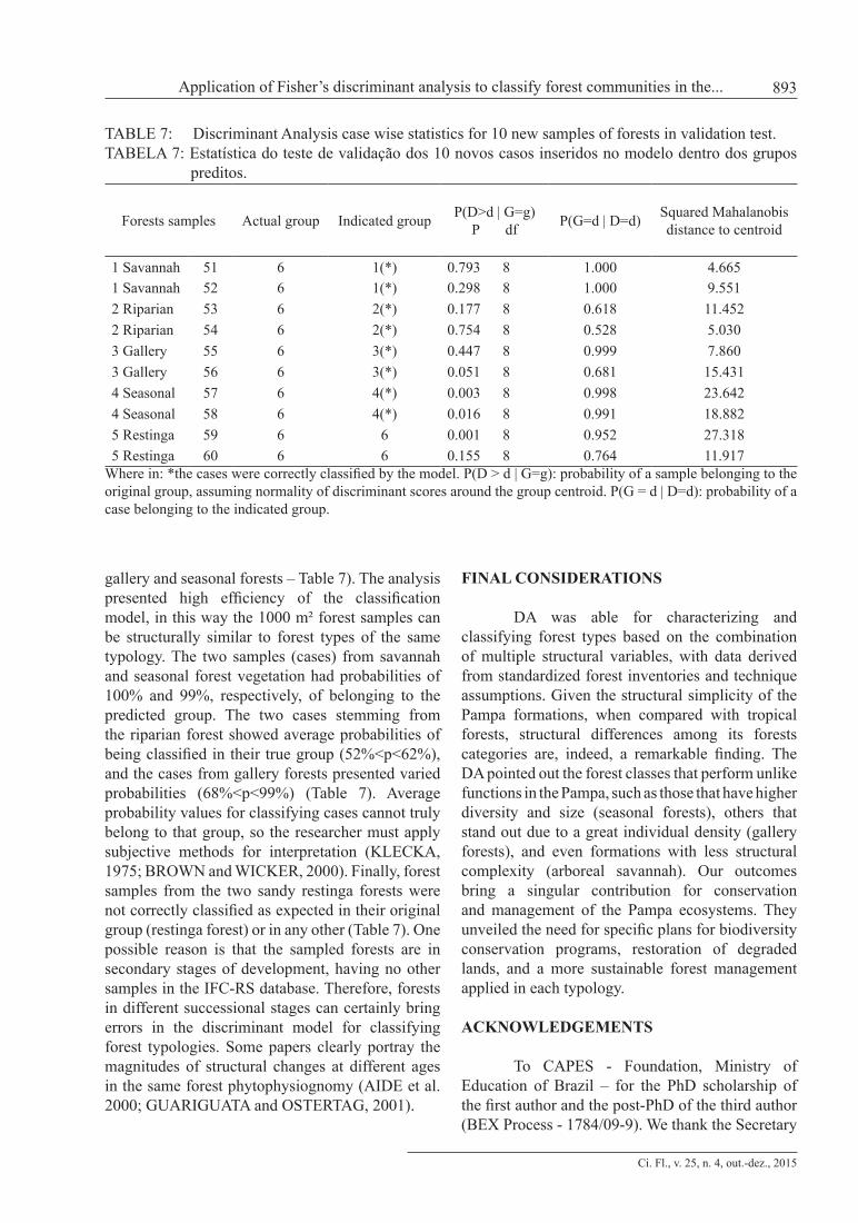
gallery and seasonal forests – Table 7). The analysis presented high efficiency of the classification model, in this way the 1000 m² forest samples can be structurally similar to forest types of the same typology. The two samples (cases) from savannah and seasonal forest vegetation had probabilities of 100% and 99%, respectively, of belonging to the predicted group. The two cases stemming from the riparian forest showed average probabilities of being classified in their true group (52%<p<62%), and the cases from gallery forests presented varied probabilities (68%<p<99%) (Table 7). Average probability values for classifying cases cannot truly belong to that group, so the researcher must apply subjective methods for interpretation (KLECKA, 1975; BROWN and WICKER, 2000). Finally, forest samples from the two sandy restinga forests were not correctly classified as expected in their original group (restinga forest) or in any other (Table 7). One possible reason is that the sampled forests are in secondary stages of development, having no other samples in the IFC-RS database. Therefore, forests in different successional stages can certainly bring errors in the discriminant model for classifying forest typologies. Some papers clearly portray the magnitudes of structural changes at different ages in the same forest phytophysiognomy (AIDE et al. 2000; GUARIGUATA and OSTERTAG, 2001).

FINAL CONSIDERATIONS

DA was able for characterizing and classifying forest types based on the combination of multiple structural variables, with data derived from standardized forest inventories and technique assumptions. Given the structural simplicity of the Pampa formations, when compared with tropical forests, structural differences among its forests categories are, indeed, a remarkable finding. The DA pointed out the forest classes that perform unlike functions in the Pampa, such as those that have higher diversity and size (seasonal forests), others that stand out due to a great individual density (gallery forests), and even formations with less structural complexity (arboreal savannah). Our outcomes bring a singular contribution for conservation and management of the Pampa ecosystems. They unveiled the need for specific plans for biodiversity conservation programs, restoration of degraded lands, and a more sustainable forest management applied in each typology.

ACKNOWLEDGEMENTS

To CAPES - Foundation, Ministry of Education of Brazil – for the PhD scholarship of the first author and the post-PhD of the third author (BEX Process - 1784/09-9). We thank the Secretary

TABLE 7: Discriminant Analysis case wise statistics for 10 new samples of forests in validation test.TABELA 7: Estatística do teste de validação dos 10 novos casos inseridos no modelo dentro dos grupos

preditos.

Forests samples Actual group Indicated group P(D>d | G=g) P df P(G=d | D=d) Squared Mahalanobis

distance to centroid

1 Savannah 51 6 1(*) 0.793 8 1.000 4.6651 Savannah 52 6 1(*) 0.298 8 1.000 9.5512 Riparian 53 6 2(*) 0.177 8 0.618 11.4522 Riparian 54 6 2(*) 0.754 8 0.528 5.0303 Gallery 55 6 3(*) 0.447 8 0.999 7.8603 Gallery 56 6 3(*) 0.051 8 0.681 15.4314 Seasonal 57 6 4(*) 0.003 8 0.998 23.6424 Seasonal 58 6 4(*) 0.016 8 0.991 18.8825 Restinga 59 6 6 0.001 8 0.952 27.3185 Restinga 60 6 6 0.155 8 0.764 11.917

Where in: *the cases were correctly classified by the model. P(D > d | G=g): probability of a sample belonging to the original group, assuming normality of discriminant scores around the group centroid. P(G = d | D=d): probability of a case belonging to the indicated group.

Ci. Fl., v. 25, n. 4, out.-dez., 2015

Kilca, R. V. et al894

of Environment of the State of Rio Grande do Sul for use of its Continuous Forest Inventory Database for Rio Grande do Sul. To the program Pró-Publicações Internacionais/PRPGP/Federal University of Santa Maria (UFSM) and the UFSM University Hospital for granting use of their computers with the SPSS 13.0 Software license. A special thanks to Dr. Fernando Hepp Pulgatti for his assistance with statistical analysis.

REFERENCES

AIDE, T. M. et al. Forest regeneration in a chronosequence of tropical abandoned pastures: Implications for restoration ecology. Restoration Ecology, vol. 8, p. 328–338, 2000.BROWN, M.T.; WICKER, L.R. 2000. Discriminant analysis, Chap. 8. In: TINSLEY, H. E. A.; BROWN, S, D. (Eds). Handbook of applied multivariate statistics and mathematical modelin. San Diego: Academic Press, 2000, p. 209-234.CABRERA, A.L.; WILLINK, A. Biogeografía de América Latina, 1st edition. Washington DC: Secretaría General de la Organización de los Estados Americanos, 1973. 120 p.DI MARCHI, T. C.; JARENKOW, J. A. Estrutura do componente arbóreo de mata ribeirinha no rio Camaquã, município de Cristal, Rio Grande do Sul, Brasil. Iheringia, Sér Bot. Porto Alegre, v. 63, n. 2, p. 241-248. 2008. DILLENBURG, L. R.; WAECHTER, J. L.; PORTO, M. L. Species composition and structure of a sandy coastal plain forest in northern Rio Grande do Sul, Brazil. In: SEELIGER, U. (Org). Coastal Plant Communities of Latin America. New York: Academic Press, p. 349-366. 1992.DORNELES, L. P. P.; WAECHTER, J. L. Fitossociologia do componente arbóreo na floresta turfosa do Parque Nacional da Lagoa do Peixe, Rio Grande do Sul, Brasil. Acta Botanica Brasilica, v. 18, n. 4, p. 815–824. 2004.FAO. Food and Agriculture Organization of the United Nations. Forest Resources Assessment 1990: Survey of tropical forest cover and study of change processes. Rome: FAO. 1996.HAIR, J.F. et al. Multivariate Data Analysis. 6nd ed. New Jersey: Prentice-Hall, 2006. 816 p. HUBERTY, C. J.; OLEJNIK, S. Applied MANOVA and Discriminant Analysis .Hoboken, New Jersey: JohnWiley & Sons Inc., 2006. 488 p.GUARIGUATA, M. R.; OSTERTAG, R. Neotropical secondary forest succession: changes in structural

and functional characteristics. Forest Ecology and Management 148: 185-206. 2001.IBGE. Instituto Brasileiro de Geografia e Estatística.. Manual Técnico da Vegetação Brasileira. Série Manuais Técnicos em Geociências - n. 1, Rio de Janeiro: IBGE, 1992. 92 p.IBGE. Instituto Brasileiro de Geografia e Estatística. Mapa da vegetação do Brasil. Available in http://www.ibge.gov.br/home/presidencia/ noticias/ noticia visualiza.php?id_ noticia=169&id_ pagina=1. Acessed 10 october 2004. JURINITZ, C. F.; JARENKOW, J. A. Estrutura do componente arbóreo de uma floresta estacional na Serra do Sudeste, Rio Grande do Sul, Brasil. Revista Brasileira de Botânica, v. 26, n. 4, p. 475-487. 2003KLECKA, W. R. Discriminant Analysis. In: NIE, N. H. et al. (Eds). Statistical Package for the Social Sciences. New York: McGraw-Hill, p. 434-467. 1975. KLEIN, R. M. Aspectos dinâmicos da vegetação no sul do Brasil. Sellowia, Itajaí, v. 36, p. 5-54. 1984. LEITE, P. F. Contribuição ao conhecimento fitoecológico do sul do Brasil. Ciência e Ambiente, Santa Maria, v. 24, p. 51-73. 2002.LINDMAN, C. A. M. Vegetação do Rio Grande do Sul (Brasil Austral). Porto Alegre: Tipografia Universal, 1906. 356 p.LOMBARDO, A. Flora Arborea y Arborescente del Uruguay. Montevideo: Consejo Departamental de Montevideo/Direccíon de Paseos Públicos, 1964.151 p.LONGHI, S. J. Aspectos fitossociológicos de uma floresta natural de Astronium balansae Engl., no Rio Grande do Sul. Ciência Rural, Santa Maria, v. 17, n. 1-2, p. 49-61. 1987.McELHINNY, C., GIBBONS, P., BRACK, C.; BAUHUS, J. Forest and woodland stand structural complexity: Its definition and measurement, Forest Ecology and Management, Amsterdam v. 218, p. 1–24, 2005.MANLY, B. F. J. Multivariate Statistical Methods: a Primer, 3rd ed. New York: Chapman & Hall, 2005. 215 p. MARCHIORI, J. N. C.; LONGHI, S. J.; GALVÃO, F. Composição florística e estrutura do Parque de Inhanduvá no Rio Grande do Sul. Ciência Rural, Santa Maria, v. 15, n. 4, p. 319-334. 1984.MARCHIORI, J. N. C.; LONGHI, S. J.; GALVÃO, F. Estrutura fitossociológica de uma associação natural de Parque Inhanduvá com Quebracho e Cina-cina, no Rio Grande do Sul. Ciência e Natura,

Ci. Fl., v. 25, n. 4, out.-dez., 2015

Application of Fisher’s discriminant analysis to classify forest communities in the... 895

Santa Maria, v. 7, n. 1, p. 147-162. 1985.OVERBECK, G. E. et al. Brazil’s neglected biome: The South Brazilian Campos. Perspectives in Plant Ecology, Evolution and Systematics, v. 9, p. 101-116. 2007.RAMBO, B. A fisionomia do Rio Grande do Sul. Porto Alegre: Selbach, 1956. 417 p.RENCHER, A. C. Methods of Multivariate Analysis. New York: Wiley, 2002. 798 p.RICHARDS, P. W. Tropical rain forest: an ecological study. Cambridge: Cambridge Univ. Press, 1952. 450 p .RIZZINI, C. T. Tratado de fitogeografia do Brasil, 2 ed. Rio de Janeiro: Ambito Cultural Edições Ltda, 1997. 747p.SEMA/UFSM. Secretaria Estadual do Meio

Ambiente/Universidade Federal de Santa Maria. 2002. Inventário Florestal Contínuo do Rio Grande do Sul. Available in http://coralx.ufsm.br/ifcrs/. Acessed 20 february 2006.THESSLER S. et al. Using k-NN and discriminant analyses to classify rain forest types in a Landsat TM image over northern Costa Rica. Remote Sensing of Environment, v. 112, n. 5, p. 2485-2494. 2008.TORTORELLI, L. A. Maderas y bosques Argentinos. Buenos Aires: ACME, 1956. 910 p.WAECHTER, J. L.; JARENKOW, J. A. Composição e estrutura do componente arbóreo nas matas turfosas do Taim, Rio Grande do Sul. Biotemas, Florianópolis, v. 11, n. 1, p: 45-69. 1998.