Application of geostatistics with Indicator Kriging for analyzing spatial variability of groundwater arsenic concentrations in Southwest Bangladesh (2011) Journal of Environmental Science and Health, Part A: Toxic/Hazardous Substances &

Environmental Engineering 46, 11, 1185-96 M. MANZURUL HASSAN1 and PETER J. ATKINS2

1 Department of Geography and Environment, Jahangirnagar University, Savar, Dhaka,

Bangladesh 2 Department of Geography, Durham University, Durham, United Kingdom

This article seeks to explore the spatial variability of groundwater arsenic (As) concentrations in Southwestern Bangladesh. Facts about spatial pattern of As are important to understand the

complex processes of As concentrations and its spatial predictions in the unsampled areas of the study site. The relevant As data for this study were collected from Southwest Bangladesh and were analyzed with Flow Injection Hydride Generation Atomic Absorption Spectrometry

(FI-HG-AAS). A geostatistical analysis with Indicator Kriging (IK) was employed to investigate the regionalized variation of As concentration. The IK prediction map shows a

highly uneven spatial pattern of arsenic concentrations. The safe zones are mainly concentrated in the north, central and south part of the study area in a scattered manner, while the contamination zones are found to be concentrated in the west and northeast parts of the

study area. The southwest part of the study area is contaminated with a highly irregular pattern. A Generalized Linear Model (GLM) was also used to investigate the relationship between As concentrations and aquifer depths. A negligible negative correlation between

aquifer depth and arsenic concentrations was found in the study area. The fitted value with 95 % confidence interval shows a decreasing tendency of arsenic concentrations with the

increase of aquifer depth. The adjusted mean smoothed lowess curve with a bandwidth of 0.8 shows an increasing trend of arsenic concentration up to a depth of 75 m, with some erratic fluctuations and regional variations at the depth between 30 m and 60 m. The borehole

lithology was considered to analyze and map the pattern of As variability with aquifer depths. The study has performed an investigation of spatial pattern and variation of As

concentrations. Keywords: Arsenic, geostatistics, GLM, Indicator Kriging, Bangladesh.

Introduction

Groundwater in Bangladesh is reportedly found to be contaminated with toxic levels of arsenic (As) that threaten the health of millions of people in Bangladesh. The impact of As poisoning on human health in Bangladesh has been alleged to be the “worst mass poisoning

in human history”.[ 1] Since the discovery ofAs in groundwater in 1993 by the Department of Public Health Engineering (DPHE), As contamination has been increasing at an alarming

rate, and the risk is spreading all over the country. The extensive use of As-contaminated groundwater for drinking and cooking threatens the health of about 70 million people in 61 out of 64 districts in Bangladesh.[2] Arsenic contaminated wells across the country are

thought to be a hazard to human health. One estimate is that millions of people may die or suffer from the very serious consequences of consuming As.[3]

There is a complex pattern of spatial variability of As concentrations in groundwater, with significant differences between neighboring wells, trends at the regional scale, and also

changes with depth underground.[4,5–10] Yu et al.[3] find a small statistically insignificant positive correlation between observed As concentrations and shallow tubewell density.

Mukherjee et al.[11] observed elevated dissolved As (>10 μg/L) in a majority of the deep groundwater samples in West Bengal, India and the maximum concentration was recorded at

137 μg/L. In addition, very little is known about changes in As concentration over time,[3] but a temporal variation of groundwater As concentrations is thought to be significant.[12–13]

The Indicator Kriging (IK) proposed by Journel[14] is one of the most efficient

nonparametric methods in geostatistics.[ 15] IK is a spatial interpolation technique devised for estimating a conditional cumulative distribution function at an unsampled location.[16] It has become the basis of some estimate algorithms and sequential indicator simulations.

Meliker et al.[17] investigated the validity of different spatial models. IK can model for estimating the probability distribution of spatial variables on the basis of surrounding

observations. In this study, an IK approach was adopted for analyzing the spatial pattern of As concentrations in Southwest Bangladesh.

Because of the distribution of groundwater As is extremely heterogeneous in both vertical and horizontal dimensions, a proper policy formulation to extract groundwater with new

tubewells is problematic. Mapping the geographical pattern of groundwater As concentrations with a spatial dimension is the focal issue of this study, and emphasis is laid on the relationships between As concentrations and aquifer depths as well as tubewell age.

Borehole lithology, the new data for this paper, is considered to analyze the pattern of As concentrations at different stratigraphy.

Earlier we reported for the same study site analyses of spatial risk fromAs poisoning andmainly focused ourwork on the spatial risk pattern of groundwater As poisoning analyzed

with Ordinary Kriging (OK) method.[18] However, in the present study described in this paper the subsurface geology of the study site has been considered with the inclusion of a

number of spatial analytical figures. Geostatistics with IK interpolation technique and Generalized Linear Model (GLM) which are the main data analysis methods were employed in order to investigate the pattern of As concentrations and its spatial variability. This spatial

variation of As concentrations will be helpful in formulating spatial policy to mitigate As poisoning in highly contaminated areas and so reducing the “health risk”.

Materials and methods

Study area and geology

The data for this study were collected from Ghona Union (the fourth-order local government administrative unit in Bangladesh) of Satkhira District in the southwest o f Bangladesh near to

the border with India (Fig. 1). The study area comprises nine administrative wards covering an area of 17.26 km2 and had a population of 13,287 in 1991.[19] The study area is geologically a part of the quaternary deltaic sediments of the Ganges alluvial and tidal

plains.[20] The surface geology of the study area mainly comprises (a) the Ganges alluvial plain, which covers the middle part of the study area (about one-third); and (b) the northern

and southern parts (two-thirds) that lies in the Ganges tidal plains. The British Khal (canal) and theMahmudpur Khal are the two main rivers flowing through the study area. The study area has been dominated by irrigated agriculture for the last few decades.

The subsurface geology of the study area has complex inter- fingerings of coarse and fine-

grained sediments from numerous regressions and transgressions throughout geologic

time.[21] The Holocene sedimentary succession, in the study area, shows a fining upward sequence from medium to fine sand, silt and finally to clay. The aquifer of this region is

mostly unconfined to leaky confined and groundwater occurs within a few meters of the surface. Two distinct aquifers occur all over the study area. The deep aquifer in the study area

is at depths of ≥144.5 meters and the shallow aquifer at depths of <144.5m (Fig. 1). The aquitard separating the shallow aquifer from the deep aquifer is a continuous one and increases in thickness towards the south and at places the thickness is about 100 m.[22] The

upper part of the shallow aquifer is comprised of fine to very fine sands and the lower part is medium to course sand. Arsenic is generally found in shallow aquifer; while the deeper

aquifer has not so far been found to be severely contaminated, other than in a few cases.

Fig. 1. The study area with lithology of a borehole: Ghona Union at Southwest Bangladesh. The borehole is located near the Ghona Union Headquarters (color figure available online).

Arsenic and attribute data

In most quantitative inquiry, the dominant sampling strategy is probability sampling. Tubewell screening is important priority work for As data collection. Which tubewells would be screened and how many? This was an important and sensitive issue in the context of

present arsenic situation in Bangladesh. Our previous experiences in this regard were taken into account, and all the tubewells were screened. Moreover, since groundwater As

concentrations are uneven in space and time dimension, all the 375 tubewells in the study area were analyzed. The geographical location of each tubewell in the study area was plotted on mouza maps (lowest level administrative territorial unit in Bangladesh) having a scale of

1:3960. Field test kits (FTK) are easy to use in analyzing groundwater As concentrations and are cost-effective, but their results are less reliable and less accurate than laboratory

methods.[13,18,23–25] In addition, FTK results are not accurate enough to permit testing at theWHOpermissible limit and sometimes even the Bangladesh DrinkingWater Standard (BDWS).

For evaluation of the reliability and accuracy of the As data, all the collected water samples

(n = 375) were analyzed with FI-HG-AAS method from the School of Environmental Studies

of Jadavpur University, Kolkata, India. To prevent adsorption losses, the collected samples were preserved by acidification with a 0.05 mL of concentrated nitric acid (14 M) in each

10mLofwater sample and placed in a refrigerator at a temperature below 4◦C prior to analysis. The method is characterized by high efficiency, low sample volume, reagent

consumption, improved tolerance of interference, and rapid determination.[26–27]With a 95 % confidence interval, the minimum detection limit of the FI-HG-AAS method is 0.001mg/L, and the quantification limit is 0.003 mg/L,[28] which is excellent for As research. Along with

the As content in water, two main attributes were collected for each tubewell: (a) tubewell depth and (b) tubewell installation year. All of the tubewell owners (375 tubewells) were

asked for information about these attributes of their tubewells through a questionnaire survey. This attribute information was stored as records (rows) in a relational database. The map features (e.g., point, line, and polygon) were used for geoststistical analysis and GIS

(Geographical Information Systems) mapping. The incorporated borehole litholog data was collected from the Department of Public Health Engineering (DPHE) office in Satkhira in

2009. The litholog data was then compiled and incorporated with arsenic concentrations, tubewell depths, aquifer depths, and age of each tubewell.

Geostatistics and indicator kriging

The geostatistical approach is a distribution-free procedure and is based on a theory of

regionalized variables whose values vary from place to place.[29–30] It relies on both statistical and mathematical methods to create surfaces and to assess the uncertainty of predictions. Geostatistics represents an appropriate method of prediction[15,31] and is widely

used for spatial estimation taking spatial variability into account.

Variogram provides a means of evaluation of the attributes in which each estimate is a weighted average of the observed values in the neighborhood. The weights mainly depend on fitting the variogram to the measured points. The variogram quantifies the spatial variability

of the random variables between two sites. The experimental variogram is fitted with a theoretical model, γ (h), which may be spherical, exponential or Gaussian, to determine the

nugget effect (C0), the sill (C0 + C1) and the range (a). The variogram can be computed in different directions to detect any spatial anisotropy of the spatial variability.[32] This study adopted a geometric anisotropic model, which yields variograms with the same structural

shape and variability (sill+nugget) but a direction-dependent range for the spatial

correlation.[33] The general equation for estimating prediction value, 0SZ

, is given by

(1) i

N

1ii0 SZλSZ

Where,

0SZ prediction value for location, 0S ;

N number of measured sample points surrounding the prediction location;

iλ the weight obtained from fitted variogram; and

iSZ observed value at location .iS

A kriging treatment quantifies the variability of As in the form of a semivariogram, which graphically expresses the relationship between the semivariance and the sampling distance.[34] The semivariogram, ˆ γ (h), is half the average squared difference between pairs

of data Z(xi) and Z(xi + h) at locations xi and xi + h. An estimate of the semivariogram with N(h) the number of sampling pairs separated by a distance of h(lag) is given by the following

equation:

)2( 2

)()()(2

1)(ˆ

)(

1

hN

i

hxZxZhN

hii

IK is an advanced nonparametric geostatistical method due to its ability to take data uncertainty into account. IK makes no assumption regarding the distributions of variables,

and a 0–1 indicator transformation of data is adopted to ensure that the predictor is robust to outliers.[35] In an unsampled location, the values estimated by IK represent the probability

that does not exceed a particular threshold. Therefore, the expected value derived from indicator data is equivalent to the cumulative distribution function of the variable.[36] IK provides an estimate of the cumulative distribution of the data set by calculating conditional

probabilities. These probabilities can be estimated by transforming the variables to a one or zero, depending upon whether they fall above or below a cutoff level:[37]

(3) . . . . . . . . . . . . . . . . . . . . . . . . . . . )( 0

)( 1);(

k

k

ZXZif

ZXZifZXi

Where, kZ is the cutoff level.

By using kriging, the interpolated indicator variable at any point X0 can be estimated by:[38]

)4( . . . . . . . . . . . . . . . . . . . . . . . . . . . . . . )()(1

00

*

n

j

jkjk XiXI

Where, *

kI the estimate of the conditional probability at jX ;

0j the kriging weight for the indicator value at point jX .

The conditional probability in this case is defined as:

(5) . . . . . . . . . . . . . . . . . . ) ., . . . . . ,1;/()( 0 njZZXZrob jK

By varying kZ , the cumulative probability can then be constructed.

IK determines the probability of the As indicator in the study area by using the samples in the neighborhood. To conduct IK, As concentrations were transformed into an indicator variable

and the variogram function was evaluated in horizontal directions to identify the anisotropic variation present in groundwater As concentrations. Some three threshold values ( i.e., the

first quartile, median and the third quartile)were selected forAs indicator analysis (Table 1). An omnidirectional variogram was used to analyze the spatial structures of As concentration. A lag increment of 1/2 km was adopted to obtain a stable variogram structure. The spatial As

probability map was analyzed and interpolated in ArcGIS (version 9.2).

The IK prediction map was developed with spherical variogram fit. The experimental variogram was computed from the As data and a mathematical model was fitted to As values

by weighted least-squares approximation. The spherical model was used to fit the raw semivariogram:[39]

(6) . . . . . . . . . . . .

0 2

1

2

3

0 0

)(ˆ

10

3

10

ahCC

aha

h

a

hCC

h

h

where, C0 is the nugget variance, and the lag, h required to reach the sill (C0 + C1) is called a

range, a. Nugget is a measure of spatial discontinuity at small distances, sill is an estimate of sample variances under assumption of spatial independence, and range is the distance at

which sample data is spatially independent. In producing prediction maps for spatial As concentrations with IK prediction method, different properties for cross-validation in terms of semivariogram and search neighbourhood were used in the interpolation (Fig. 2).

Generalized linear models

The GLM was used to identify the association between As concentrations and aquifer depths as well as tubewell installation age. The GLM is a mathematical extension of linear models that do not force data into unnatural scales, and thereby allow for non- linearity and non-

constant variance structures in the data.[40–43] They are based on an assumed relationship (link function) between the mean of the response variable and the linear combination of the

explanatory variables. Hypothesis testing applied to the GLM does not require normality of the response variable, nor does it require homogeneity of variances. Since As data are not distributed normally, the GLM was used for this paper. The maximum likelihood estimation

technique is an important advent in the development of GLM.[42] TheNewton-Raphson (maximumlikelihood) optimization technique was used in this paper to estimate the GLM and

the STATA statistical software was utilized to calculate the GLM.

Performance assessment

In the prediction maps of arsenic concentrations, cross validation was used to compare the prediction performance of the IKinterpolation algorithm (Fig. 2). Cross-validation indicators

and the model parameters (nugget, sill, and range) help us to choose a suitablemodel for the prediction maps of arsenic concentrations. In the procedure, arsenic concentration is

estimated successively for each sampled tubewell using the known neighbours. The cross-validation was applied to improve and to control the quality of the applied geostatistical model and thus the results of the spatial analysis. The differences between measured and

predicted values provide a quality control for the model of computation for arsenic concentrations. The difference between measured and estimated values was obtained by cross

validation. Based on the cross-validation results of the data exploration and the variogram analysis, the measured data are converted to surface maps. IK is used to divide values at locations to three different categories by means of a threshold limits. The observed values

Z(U) are then compared with the interpolated ones Z* (U) using the performance measures the bias:[44]

And the root mean square error normalized with the observed average:[44]

Interpolation usually leads to a smoothing of the observations and thus to a loss of variance.

In analyzing the data with IK prediction method, we found the average standard error of arsenic data to be 0.3903 with root mean square of 0.3964. The figures for mean standardized error were analyzed by −0.0034 and 1.023 for root mean square standardized. Figure 2 shows

the details about the prediction error of arsenic concentrations with the IK prediction method.

Results and discussion

Scale of arsenic concentrations

There has been a heterogeneous distribution of groundwater As concentration in the study

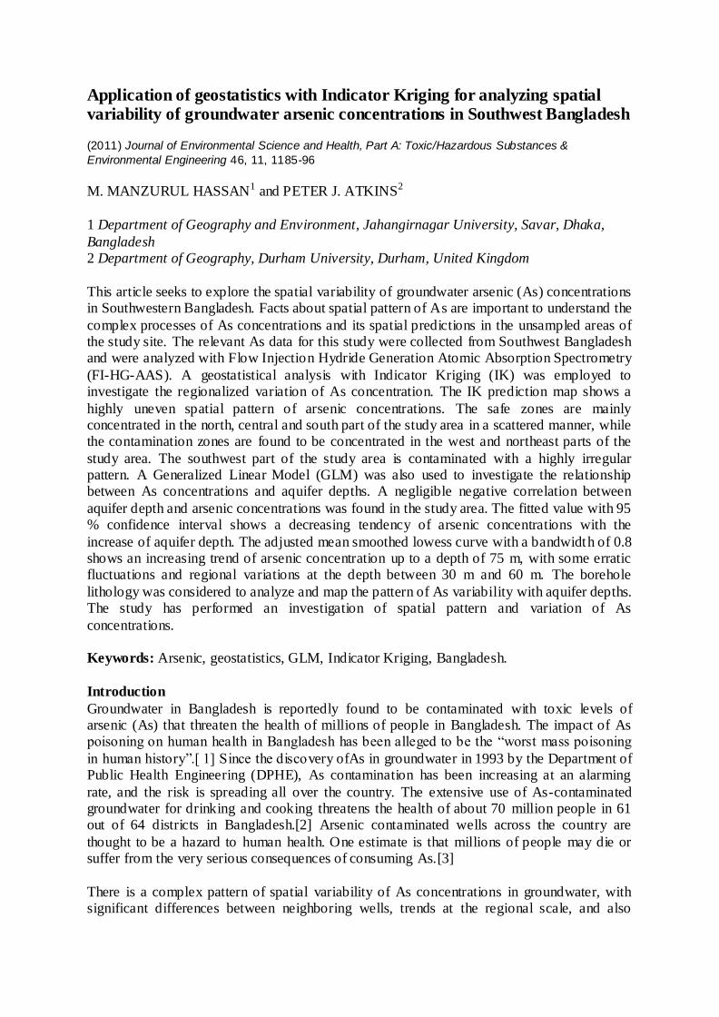
area (Fig. 3). The term “contamination” in this article refers to the elevated concentrations of As above the BDWS. Arsenic concentrations in the study area range between 0.003 mg/L and 0.600 mg/L with a mean concentration of 0.238 mg/L and the standard deviation of 0.117

mg/L. [18] The study shows that only 4.50 % of the sample tubewells (17 out of 375) belong to the safe level and 95.5 % (358 out of 375) are said to be contaminated with As ≥0.05 mg/L

(Table 2). In the safe band, only four tubewells meet the WHO permissible limit (<0.01 mg/L) and 13

tubewells qualify at the BDWS (Table 2). In addition, in the contamination category, As concentrations range between 0.057 mg/L and 0.600 mg/L with a mean concentration of

0.248 mg/L and standard deviation (δn) of 0.109 mg/L (Table 2). It is noteworthy that the mean As concentration in this contamination category is 5 times higher than the BDWS and 25 times higher than the WHO permissible limit. [18] The pattern of concentrations varies

considerably and unpredictably over distances of a few meters, notably about 46 % of tubewells are located within 25 m of each other within the settlement area of the study

site.[18] The measured As concentrations are 0.1405 mg/L, 0.241 mg/L and 0.3267 mg/L at the first,

second (median) and the third quartile of the frequency distribution of As concentrations (Table 1). The omnidirectional variogram was adopted to analyze the geometric anisotropic

variability. The anisotropic ratios (maximum range/minimum

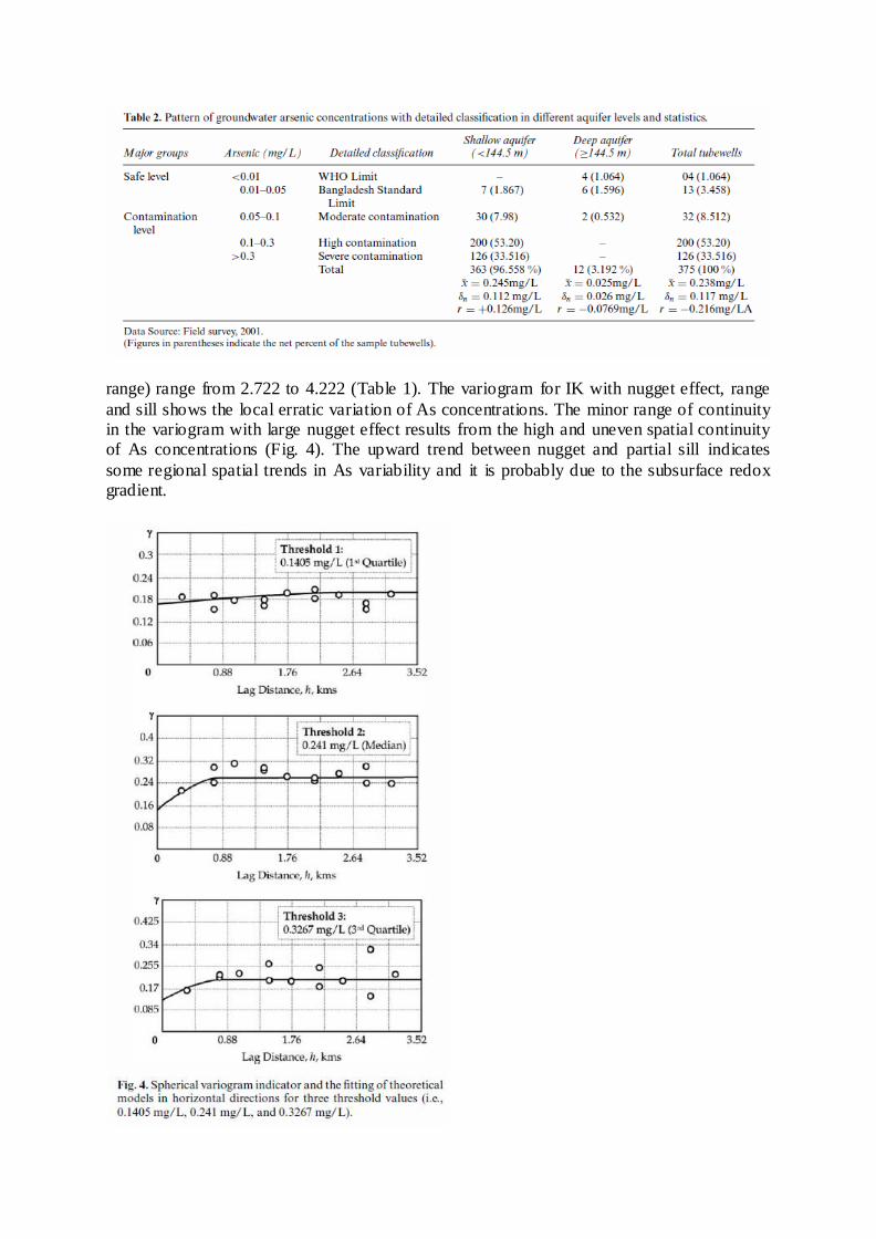
range) range from 2.722 to 4.222 (Table 1). The variogram for IK with nugget effect, range

and sill shows the local erratic variation of As concentrations. The minor range of continuity in the variogram with large nugget effect results from the high and uneven spatial continuity of As concentrations (Fig. 4). The upward trend between nugget and partial sill indicates

some regional spatial trends in As variability and it is probably due to the subsurface redox gradient.

The probability map developed with the IK prediction method shows a highly uneven spatial

pattern of As concentrations (Fig. 5). It is noted here that Figure 5 was prepared with IK prediction method. Three different threshold limits for As concentrations were used to

develop the maps for Figure 5. Table 1 shows the details regarding this issue. Different threshold limits show different patterns of spatial As continuity in the study area (Fig. 5). There are visible discrepancies in spatial continuity of As concentrations in the central and

eastern parts of the study area and the pattern is very uneven. The safe zones are mainly concentrated in the north, central and south part of the study area in a scattered manner. The

central part of the study area is found to be low contaminated - in an area roughly corresponding to the Ganges alluvial floodplain. Contamination zones are found everywhere in the study area but with a decrease in the degree of contamination from west to east: they

are largest in the low-lying area of the west and north-east. The south and southeast regions appear to show safe zones with some local variability. The west and northeast parts of the

study area are mostly contaminated; while the southwest part of the study area is contaminated with a highly irregular pattern (Fig. 5). The safe zones are associated with the highest elevations of the area, and the contamination zones are on the west and northeast part

where the elevation is low and agriculture predominant.

Arsenic concentrations with depth

Arsenic concentrations in the study area are highly uneven with depth (Fig. 6a). Tubewell

depths range between 18 m and 200 m. Drawing upon the shallow aquifer (≤144.5 m) and deep aquifer (>144.5 m), about 97 % (n = 363) and 3.0 % (n = 12) tubewells have been

recognized respectively (Table 2). The aquifer below the second aquitard is generally defined as the deep aquifer; while aquifer located in between the first and second aquitards is known as the shallow aquifer. The second aquitard is located between 92.0 and 144.5 m depth in the

study site (Fig. 1). Of those using the shallow aquifer, only 1.87 % cent of the tubewells (n = 7) were found to be safe and about 94.7 % (n = 356)were contaminated,with amean

concentration of 0.254 mg/L (Table 2). Moreover, in the deep aquifer, only eight tubewells (out of 12) failed the WHO standard and two tubewells failed the BDWS (Table 2). A negligible negative correlation between aquifer depth and As concentrations was found in the

study area. The product moment of correlation value (r = −0.216) shows that there is a slow

decreasing tendency of As concentrations with increase of aquifer depth. The fitted value with 95%confidence interval shows a decreasing tendency ofAs concentrations with the

increase of aquifer depth, but As concentration levels are low in tubewells tapping the deep

aquifer. In addition, the adjusted mean smoothed lowess curve with a bandwidth of 0.8 shows an increasing trend of As concentration up to a depth of 75 m, with some erratic fluctuations

and regional variations at the depth between 30 and 60 m (Fig. 7a).

Marked regional variations and a considerable contrast in As concentrations are noticeable in the sub-surface geology (Table 3). Arsenic concentrations in the ‘fine sand zone’ (depth: 42.7–49.2 m) range from 0.032 mg/L at 45 m depth to 0.535 mg/L at 46mdepth, with amean

concentration of 0.219 mg/L for 85 tubewells. In the ‘very fine sandy zone’ (depth: 49.3–65.6m), the value ranges between 0.032 mg/L at 51mdepth and 0.515 mg/L at 55mdepth with

themean concentration of 0.243 mg/L for about two-fifths (n = 153) of the total sample tubewells. At the depth of 65.7–91.9 m (fine to medium sandy zone), As concentrations range between 0.011 mg/L at 85 m depth and 0.600 mg/L at 71m depth, having a mean

concentration of 0.264 mg/L for 105 tubewells (Table 3).

It was found that the pattern of As concentration varies with grain-size distribution and that

there is a lithological relationship with As concentrations. The ‘r ’ values show very negligible positive associations between As concentrations at depths 42.7–49.2 m and 49.3–

65.6 m; while a negligible negative association was found at depths of 65.7–91.9 m (Table 3). Arsenic concentrations were also found to be highly uneven at certain depths (Fig. 8). At a

depth of 42 m, a sharp variation in As concentrations was identified in 51 tubewells having a range between 0.034 and 0.428 mg/L, with a mean concentration of 0.2035 mg/L. At a depth

of 55 m, a substantial variability in As concentrations for 28 tubewells was found: between 0.037 and 0.515 mg/L. At a depth of 74 m, a sharp variation was also identified in 25 tubewells having a range between 0.069 and 0.392 mg/L. Some nine tubewells have been

found within a 135 m radius in the southern part of the study area that have values between 0.142 and 0.241 mg/L; while at a depth of 180 m, dissimilarity in As concentrations was

found for seven tubewells having a range between 0.003 to 0.093 mg/L (Fig. 8).

Arsenic concentrations were found to be declining with tubewell age, although the

concentration pattern is uneven and erratic over different time periods (Fig. 6b). Tubewells were first installed in the study area in 1950 and there were only six tubewells prior to the 1971 LiberationWar. The figure increased to 375 by mid 2001. No tubewells were found to

be safe that had been installed prior to 1981. The very low negative association (r = −0.209) shows a slight decreasing pattern of As concentrations over time. The fitted line with 95 %

confidence interval shows a declining trend of As concentrations over time. In addition, the adjusted mean smoothed lowess curve (bandwidth 0.8) shows a declining pattern of relationship between tubewell age and As concentrations. The lowess smoothed line also

shows an erratic pattern for recently installed tubewells (Fig. 7b). Tubewell installation year is not a proxy of As concentration dynamics over time since the different concentrations

could be location-dependent and not just time-dependent. This can be assessed only within the framework of a monitoring program aimed to assess As concentration in time for given

wells. In this paper As concentration is measured only at one point in time, so it is hard to come to conclusive statements in terms of temporal dynamics.

Discussion

The IK prediction map shows a highly irregular and diverse pattern of As concentration in the study area. A line of evidence shows very high uneven groundwater As concentrations over space.[45–46] About half (46 %) and more than one-fourth (28 %) of the analyzed tubewells

measured by atomic fluorescence spectrometry were found to be contaminated with As having the WHO permissible limit and the BDWS respectively and found variation with

spatial characteristics having both small-scale variability and large-scale trends.[47] In addition, it was found that almost half of the surveyed 6000 tubewells in Araihazar failed the BDWS for As.[4]

Evidence shows that deep aquifers are almost free from As, but in Bangladesh, only 1 % of

tubewells deeper than 200 m have As above 0.05 mg/L and only 5 % exceeded 0.1 mg/L of As.[47] Arsenic is also commonly absent in wells at shallow depths (<5 m), especially in dug wells.[48] In our study, we found that 75 % of the deep tubewells failed to comply WHO

standard. At a depth of 12–24 m, themaximumnumber of tubewells was found to be concentrated with As frequently exceeding the BDWS.[4] Harvey et al.[45] showed in their

study that dissolved As has a distinct peak at approximately 30 m depth; while Jakariya et al.[13] show a robust association between As concentrations and aquifer depth between 30 and 76 m. A number of studies show typical depth profiles of As concentrations to be “bell-

shaped”.[4,49–50] Depth trends can be considered within different geologic regions and Yu et al.[3] show a statistically significant trend of decreasing As with depth in different

geologic regions of Bangladesh. Our study shows that As concentration is higher in the fine to medium sediments of the study

site. Concurrently, Ahmed et al.[51] and Burges and Ahmed[48] show that As source is preferentially concentrated within fine-grained sediments; while Jakariya et al.[13] argue that

a high As concentration is visible at aquifer levelswith the dominance of medium-sized sediments. However, Sharif et al.[8] claim that medium- to coarse-grained aquifer sands are generally less heterogeneous and have a spatially uniform As content. Moreover, Harvey et

al.[49] and Swartz et al.[52] note that no chemical characteristics of the solid sediment could be found to explain the high variation of As concentrations with aquifer depth. Spatial

variability of groundwater As concentrations is influenced by lithologic heterogeneity, which is controlled by sediment geochemistry, recharge potential, thickness of surface aquitard, local flow dynamics, and the degree of reducing conditions in the aquifer.[8] This incongruity

in the relation between grain size and As concentrations might result from the textural properties of the aquifer sands at different depths and aquifer chemistry. It should be noted

that a tubewell presently As-free or having an acceptable As concentration cannot be relied upon for long because of the paradoxical nature of concentrations in different space-time dimensions. The literature shows that older wells have a higher probability of high

concentrations of As in water. A BGS/DPHE[47] report indicates that those tubewells shallower than 150 m, which contain As at >0.05 mg/L increases consistently with time. A

general trend of increasing As concentration with the duration of pumping at individual tubewells was also noticed.[ 53–55] Nath et al.[56] demonstrate a decreasing trend of As concentration with depth, except for a slight increase observed between 70 and 80 m depth.

However, deeper groundwater (>80 m depth) is not entirely free from As. This contradicts the previously reported As distribution scenario in the Bengal Delta Plain.[47,57] These

observations imply that As is not released to groundwater uniformly with depth.[58] The

potential for a deep water supply depends on aquifer depth and the lateral extent of a substantial aquitard and its vertical profiles of permeability, coherence, and occurrence of

aquitard.

Conclusion

Analysis of the groundwater As concentrations in the study area reveals the significant spatial variability of As. The IK prediction map shows low As concentrations in the north, central

and south part of the study area in a scattered manner. The west and northeast of the study area are generally more contaminated, while the southwest part of the study area is

contaminated in a highly irregular pattern. The calculated nugget effects, ranges and sills have shown locally erratic variations of As concentrations in the study area. The study has also investigated the deviating relationships between aquifer depths and As concentrations. A

low negative association was found for aquifer depths and As concentrations. Deep tubewells were also found to be contaminated, but at a low level of concentration. Associations of As

with lithology have also been examined over small regional scales and indicate widespread occurrences of As in the alluvial aquifers that are controlled by larger geological and hydrogeological features.

The spatial pattern of As concentrations in the study area does not show any uniformity

corresponding to surface geology. This unevenness in As concentration is due to the aquifer characteristics and surface geology. The study shows thatGanges-deltaic flood plain deposits contain very high and erratic concentrations of As. The sharp microlevel variation of As

concentrations in the same aquifer raises a number of issues. Is geological variability the main cause of the differences? The variation ofAs concentrations over time also raises the

issue of the mechanism of As in Bangladesh groundwater. What are the reasons for the variation of As concentration with tubewell age: heavy

withdrawal of groundwater for irrigation and domestic uses, or according to geological origin and lithology? Therefore, more research is needed on spatio-temporal analysis, more

specifically depth-specific distribution in different geological settings to investigate the nature of As mobilization. Moreover, there is a need to investigate the role of organic matter in the mechanism of As release in groundwater.

Acknowledgments

The senior author would like to express his sincere thanks to Professor Dipankar Chakraborti of the SOES, Jadavpur University, Kolkata, India for his cooperation in the laboratory analysis of the water samples. In addition, we are grateful to three anonymous referees for

their constructive remarks.

References

[1] Smith, A.H.; Lingas, E.O.; Rahman, M. Contamination of drinking-water by arsenic in Bangladesh: a public health emergency. Bulletin of the World Health Organization 2000, 78,

1093–1103. [2] Stute, M.; Zheng, Y.; Schlosser, P.; Horneman, A.; Dhar, R.K.; Hoque, M.A.; Seddique,

A.A.; Shamsudduha, M.; Ahmed, K.M.; van Geen, A. Hydrological Control of As Concentrations in Bangladesh Groundwater. Water Resour. Res. 2007, 43. [3] Yu, W.H.; Harvey, C.M.; Harvey, C.F. Arsenic in groundwater in Bangladesh: a

geostatistical and epidemiological framework for evaluating health effects and potential remedies.Water Resour. Res. 2003, 39 (6), 1146.

[4] van Geen, A.; Zheng, Y.; Vesteeg, R.; Stute, M.; Horneman, A.; Dhar, R.; Steckler, M.; Gelman, A.; Ahsan, H.; Graziano, J.H.; Hussain, I.; Ahmed, K.M. Spatial variability of

arsenic in 6000 tubewells in a 25 km2 area of Bangladesh.Water Resour. Res. 2003, 39 (5), 1140.

[5] Ghosh, A.; Sarkar, D.; Dutta, D.; Bhattacharyya, P. Spatial variability and concentration of arsenic in the groundwater of a region in Nadia district, West Bengal, India. Arch. Agron. Soil Sci. 2004, 50, 521–527.

[6] Hossain, F.; Sivakumar, B. Spatial pattern of arsenic contamination in shallow wells of Bangladesh: Regional geology and nonlinear dynamics. Stochast. Environ. Res. Risk Assess.

2005, 20 (1–2), 66–76. [7] Peters, S.C.; Burkert, L. The occurrence and geochemistry of arsenic in groundwaters of the Newark basin of Pennsylvania. Appl. Geochem. 2008, 23, 85–98.

[8] Sharif, M.U.;Davis,R.K.; Steele, K.F.;Kim, B.; Hays, P.D.; Kresse, T.M.; Fazio, J.A. Distribution and variability of redox zones controlling spatial variability of arsenic in the

Mississippi River Valley alluvial aquifer, southeastern Arkansas. J. Contam. Hydrol. 2008, 99 (1–4), 49–67. [9] Smedley, P.L.; Nicolli, H.B.; Macdonald, D.M.J.; Barros, A.J.; Tullio, J.O.

Hydrogeochemistry of arsenic and other inorganic constituents in groundwaters from La Pampa, Argentina. Appl. Geochem. 2002, 17, 259–284.

[10] Wang, S.W.; Liu, C.W.; Jang, C.S. Factors responsible for high arsenic concentrations in two groundwater catchments in Taiwan. Appl. Geochem. 2007, 22, 460–476. [11] Mukherjee, A.; Fryar, A.E.; Scanlon, B.R.; Bhattacharya, P.; Bhattacharya, A. Elevated

arsenic in deeper groundwater of the western Bengal Basin, India: Extent and controls from regional to local scale. Appl.Geochem. 2011, doi:10.1016/j.apgeochem.2011.01.017 (in

press). [12] Nadakavukaren, J.J.; Ingermann, R.L.; Jeddeloh, G.; Falkowski, S.J. Seasonal variation of arsenic concentration in well water in Lane County, Oregon. Bull. Environ. Contam.

Toxicol. 1984, 33, 264–269. [13] Jakariya, M.; Bhattacharya, P.; Hassan, M.M.; Ahmed, K.M.; Hasan, M.A.; Nahar, S.

Temporal Variation of Groundwater Arsenic Concentrations in Southwest Bangladesh. In Natural Arsenic in Groundwater of Latin America - Occurrence, health impact and remediation; Bundschuh, J.;Armienta, M.A.;Birkle, P.;Bhattacharya, P.; Matschullat, J.;

Mukherjee, A.B.; eds.; Interdisciplinary Book Series: Arsenic in the Environment Volume 1, Bundschuh, J.; Bhattacharya, P. (Series Editors), CRC Press/Balkema, Leiden, The

Netherlands, 2009, 225–233. [14] Journel, A.G. Nonparametric estimation of spatial distributions. Math. Geol. 1983, 15, 445–468.

[15] Bastante, F.G.; Ord´o˜ nez, C.; Taboada, J.; Mat´ıas, J.M. Comparison of indicator kriging, conditional indicator simulation and multiplepoint statistics used to model slate

deposits. Engin. Geol. 2008, 81, 50–59. [16] Braimoh, A.K.; Onishi, T. Geostatistical techniques for incorporating spatial correlation into land use change models. Int. J. Appl. Earth Observ. Geoinform. 2007, 9, 438–446.

[17] Meliker, J.R.; AvRuskin, G.A.; Slotnick, M.J.; Goovaerts, P.; Schottenfeld, D.; Jacquez, G.M.; Nriagu, J.O. Validity of spatial models of arsenic concentrations in private well water.

Environ. Res. 2008, 106, 42–50. [18] Hassan, M.M.; Atkins, P.J.; Dunn, C.E. The spatial pattern of risk from arsenic poisoning: a Bangladesh case study. J. Environ. Sci. Health, Part A, 2003, A38 (1), 1–24.

[19] BBS. Bangladesh Population census (1991) Thana Statistics. Bangladesh Bureau of Statistics, Dhaka, Bangladesh, 1991.

[20] Dowling, C.B.; Poreda, R.J.; Basu, A.R.; Peters, S.L.; Aggarwal, P.K. Geochemical study of arsenic release mechanisms in the Bengal Basin groundwater. Water Resour. Res.

2002, 38, 1173– 1190. [21] Umitsu, M. Late Quaternary sedimentary environments and landforms in the Ganges

Delta. Sedi. Geol. 1993, 83, 177–186. [22] DPHE/DfID/JICA. Development of Deep Aquifer Database and Preliminary Deep Aquifer Map (First Phase), Dhaka, Bangladesh, 2006.

[23] Durham, N.; Kosmus, W. Analytical considerations of arsenic contamination inwater. Paper presented at the 28thWEDCConference (Sustainable Environmental Sanitation and

Water Services), 2002, Kolkata, India. [24] Rahman, M.M.; Mukherjee, D.; Sengupta, M.K.; Chowdhury, U.K.; Lodh,D.; Chanda, C.R.;Roy, S.; Selim,M.; Quamruzzaman, Q.; Milton, A.H.; Shahidullah, S.M.; Rahman,

M.T.; Chakraborti, D. Effectiveness and reliability of arsenic field testing kits: are the million dollar screening projects effective or not? Environ. Sci. Technol. 2002, 36, 5385–5394.

[25] Erickson, B.E. Field kits fail to provide accurate measure of arsenic in groundwater. Environ. Sci. Technol. 2003, 37, 35A–38A. [26] Le, X.C.; Cullen, W.R.; Reimer, K.J.; Brindle, I.D. A new continuous hydride generator

for the determination of arsenic, Antimony and tin by hybride generation atomic absorption spectrometry. Anal. Chim. Acta 1992, 258, 307–315.

[27] Samanta, G., Chakraborti, D. Flow injection atomic absorption spectrometry for the standardization of arsenic, lead and mercury in environmental and biological standard reference materials. Fres. J. Anal. Chem. 1997, 357, 827–832.

[28] Samanta, G.; Roy Chowdhury, T.; Mandal, B.K.; Biswas, B.K.; Chowdhury, U.K.; Basu, G.K.; Chanda, C.R.; Lodh, D.; Chakraborti, D. Flow injection hydride generation

atomic absorption spectrometry for determination of arsenic in water and biological samples from arsenic-affected districts of West Bengal, India, and Bangladesh. Microchem. J. 1999, 62, 174–191.

[29] Journel, A.G.; Huijbregts, C.J. Mining Geostatistics. Academic Press, San Diego, 1978. [30] Isaaks, E.H.; Srivastava, R.M. An Introduction to Applied Geostatistics. Oxford

University Press, New York, 1989. [31] Xu, C.; He, H.S.; Hu, Y.; Chang, Y.; Li, X.; Bu, R. Latin hypercube sampling and geostatistical modeling of spatial uncertainty in a spatially explicit forest landscape model

simulation. Ecol. Model. 2005, 185, 255–269. [32] Lee, J.J.; Jang, C.S.; Wang, S.W.; Liu, C.W. Evaluation of potencial health risk of

arsenic-affected groundwater using indicador kriging and dose response model. Sci. Total Environ. 2007, 384, 151–162. [33] Deutsch, C.; Journel, A. GSLIB: geostatistical software library and user’s guide. Oxford

University Press, New York, 1998. [34] Srivastava, R.M. Describing spatial variability using geostatistical analysis In

Geostatistics for Environmental and Geotechnical Applications ; Rouhani. S.; Srivastava, R.M.; Desbarats, A.J.; Cromer, M.V.; Johnson, A.I.; eds; American Society for Testing and Materials, Ann Arbor, MI; 1996.

[35] Cressie, N. Fitting variogram models by weighted least square. Math. Geol. 1985, 17 (5), 563–586.

[36] Smith, J.L.; Halvorson, J.J.; Papendick, R.I. Usingmultiple-variable indicator kriging for evaluating soil quality. Soil Sci. Soc. Amer. J. 1993, 57, 743–749. [37] Sullivan, J. Conditional recovery estimation through probability kriging theory and

practice. In Geostatistics for Natural Resources Characterization, Part I; Verly,G.; David, K.; Journel, A.G.; Marechel, A.; eds.; Dordrecht, Reidel Publishingompany, 1984; 365–384.

[38] Wild, M.R.; Rouhani, S. Effective use of field screening techniques in environmental investigations: A multiple geoststistical approach. In Geostatistics for Environmental and

Geotechnical Applications; Rouhani, S.; Srivastava, R.M.; Desbarats, A.J.; Cromer, M.V.; Johnson, A.I., eds.; Ann Arbor, American Society for Testing and Materials, 1996.

[39] Chang, Y.H.; Scrimshaw, M.D.; Emmerson, R.H.C.; Lester, J.N. Geostatistical analysis of sampling uncertainty at the Tollesbury Managed Retreat site in Blackwater Estuary, Essex, UK: Kriging and cokriging approach to minimise sampling density. Sci. Total Environ. 1998,

221, 43–57. [40] Jin, M.; Fang, Y.; Zhao, L. Variable selection in generalized linear models with

canonical link functions. Stat. Probabil. Lett. 2005, 71, 371–382. [41] Khuri, A.I. An overview of the use of generalized linear models in response surface methodology. Nonlin. Anal. 2001, 47, 2023–2034.

[42] McCullagh, P.; Nelder, J.A. Generalized Linear Models. London: Chapman and Hall, 1989.

[43] Nelder, J.A.; Wedderburn, R.W.M. Generalized linear models. J. Roy. Stat. Soc. Series A 1972, 135, 370–384. [44] Haberlandt, U. Geostatistical interpolation of hourly precipitation from rain gauges and

radar for a large-scale extreme rainfall event. J. Hydrol. 2007, 332, 144–157. [45] Harvey, C.F.; Ashfaque, K.N.; Yu, W.; Badruzzaman, A.B.M.; Ali, M.A.; Oates, P.M.;

Michael, H.A.; Neumann, R.B. Beckie, R.; Islam, S.; Ahmed, M.F. Groundwater dynamics and arsenic contamination in Bangladesh. Chem. Geol. 2006, 228, 112– 136. [46] Lin, Y.B.; Lin, Y.P.; Liu, C.W.; Tan, Y.C. Mapping of spatial multiscale sources of

arsenic variation in groundwater onChiaNan floodplain of Taiwan. Sci. Total Environ. 2006, 370, 168–181.

[47] BGS/DPHE. Arsenic contamination of groundwater in Bangladesh. Vol. 2: Final Report. BGS Technical Report WC/00/19. British Geological Survey and Department of Public Health Engineering, Ministry of Local Government, Rural Development & Co-operatives,

Government of Bangladesh, 2001. [48] Burges, W.; Ahmed, K.M. Arsenic in aquifers of the Bengal Basin: From sediment

source to tube-wells used for domestic water supply and irrigation. In Managing Arsenic in the Environment: From Soil to Human Health; Naidu, R.; Smith, E.; Owens, G.; Bhattacharya, P.; Nadebaum, P.; eds; CSIRO Publishing, Victoria (Australia), 2006.

[49] Harvey, C.F.; Swartz, C.H.; Badruzzman, A.B.M.; Keon-Blute, N.; Yu, W.; Ali, M.A.; Jay, J.; Beckie, R.; Niedan, V.; Brabander, D.; Oates, P.M.; Ashfaque, K.N.; Islam, S.;

Hemond, H.F.; Ahmed, M.F. Arsenic mobility and groundwater extraction in Bangladesh. Science 2002, 298, 1602–1606. [50] McArthur, J.M.; Banerjee, D.M.; Hudson-Edwards, K.A.;Mishra, R.; Purohit, R.;

Ravenscroft, P.; Cronin, A.; Howarth, R.J.; Chatterjee, A.; Talukder, T.; Lowry, D.; Houghton, S.; Chadha, D.K. Natural organic matter in sedimentary basins and its relation to

arsenic in anoxic ground water: the example of West Bengal and its worldwide implications. Appl. Geochem. 2004, 19, 1255– 1293. [51] Ahmed, K.M.; Bhattacharya, P.; Hasan, M.A.; Akhter, S.H.; Alam, S.M.M.; Bhuyian,

M.A.H.; Imam, M.B.; Khan, A.A.; Sracek, O. Arsenic contamination in groundwater of alluvial aquifers in Bangladesh: An overview. Appl. Geochem. 2004, 19, 181– 200.

[52] Swartz, C.H.; Blute, N.K.; Badruzzman, B.; Ali, A.; Brabander, D.; Jay, J.; Besancon, J.; Islam, S.; Hemond, H.F.;Harvey,C.F. Mobility of arsenic in a Bangladesh aquifer: Inferences fromgeochemical profiles, leaching data, and mineralogical characterization. Geochim. Acta

2004, 68 (22), 4539–4557. [53] Cobbing, J. The spatial variation of arsenic in groundwater at Magura, western

Bangladesh. MSc thesis (unpublished) University College, London, 2000.

[54] Mather, S. The vertical and spatial variability of arsenic in the groundwater of Chaumohani, Southeast Bangladesh. MSc thesis (unpublished), University College, London,

1999. [55] McCarthy, E.M.T. Spatial and depth distribution of arsenic in groundwater of the

Bengal Basin. MSc thesis (unpublished), University College, London, 2001. [56] Nath, B.; Chakraborty, S.; Burnol, A.; St¨uben, D.; Chatterjee, D.; Charlet, L. Mobility of arsenic in the sub-surface environment: An integrated hydrogeochemical study and

sorption model of the sandy aquifer materials. J. Hydrol. 2009, 364, 236– 248. [57] Bhattacharya, P.; Chatterjee, D.; Jacks, G. Occurrence of arsenic contaminated

groundwater in alluvial aquifers from delta plains, Eastern India: options for safe drinkingwater supply.WaterResour. Develop. 1997, 13, 79–92. [58] Bhattacharya, P.; Rahman, S.N.; Hossain,M.; Robinson, C.; Nath, B.; Rahman, M.;

Islam, M.M.; von Br ¨omssen, M.; Ahmed, K.M.; Chowdhury, D.; Rahman, M.; Persson, L.A.; Vahter, M. Trends in arsenic distribution in drinking water wells in Matlab, SE

Bangladesh:Apreliminary evaluation on the basis of a 4 year study. J. Environ. Sci. Health Pt. A (this volume).