Application of Graphic LASSO in Portfolio

Optimization

Yixuan Chen 158000258

Mengxi Jiang 160005688

Abstract

We used graphical lasso to estimate the precision matrix of stocks in the US stock

market and apply optimization to get portfolio. The graphical lasso is compared with

other estimation methods, sample covariance and shrinkage. And we find graphical

lasso has an excellent performance in the test data.

I. Introduction:

The Least Absolute Shrinkage and Selection Operator is also called LASSO. It is

a regression method that adds a constraint on the OLS in the regression. It makes the

sum of all absolute coefficients less than a tuning parameter t. When t is large, the

constraint may not have any influence on regression. However, by penalizing the

absolute size of the regression coefficients, you may push some of the parameter

estimates to zero when tuning parameter t is small. The smaller t is, the stronger

constraint is.

Graphic lasso is the expansion of lasso. However, it is not used on regression. It is

used to estimate the precision matrix. Shared the same penalized idea with lasso,

graphical lasso needs a constraint on the minimization. When tuning parameter t is

large, the constraint may not have any influence. However, when t is small, some

elements cij in precision matrix C = Σ−1 may be pushed to zero. The precision

matrix will become a sparse matrix. Graphical lasso is usually used to estimate a

sparse inverse covariance matrix. Besides, with the usage of coordinate descent

procedure, graphical lasso is significantly faster.

In past a few years, many scholars did research on the graphical lasso.

Meinshausen and Buhlmann (2006) suggested a simpler method for covariance

selection that can be used for very large Gaussian graphs. Using their method, we can

always estimate the non-zero elements in precision matrix. Besides them, other new

articles proposed different attractive algorithms to execute the Glasso estimation.

Yuan and Lin (2007), Banerjee and others (2007), and Dahl and others (2007) dealt

with maximization with penalized log-likelihood. Specifically, Yuan and Lin (2007)

used l1 penalty on cij, which is like what lasso did in a linear regression. l1 penalty

would push the concentration matrix to be sparse and then estimated this sparse

matrix. On the foundation of previous researches, Friedman, Hastie and Tibshirani

(2008) proposed another method to do the graphical lasso. the blockwise coordinate

descent approach is involved here in order to make calculation faster and at same time

explain the "conceptual gap". Besides, witten, Friedman and Simon (2011) presented

a condition for getting a related element in graphical lasso. The condition often was

neglected before.

In our project, the algorithm we use is the algorithm Yuan and Li proposed in

2007. The reason we use it over others is that it is sampler, faster and more efficient.

Their algorithm combines the positive definite constraint and the application of

likelihood. At present, most of the research on lasso is not on the field of finance.

Hence we try to apply graphical lasso to find the concentration matrix estimator Σ−1

and make the setting of portfolio optimization good. After we get the performance of

graphical lasso in portfolio, we try to find trading strategy and make money.

We want to estimate the concentration matrix C = Σ−1. Then use C to optimize

portfolio. The interesting part here is that we try to identify some part in C as zero.

II. Technical Description

We assume X = (X1, X2, … , Xn) is a n-dimensional random vector. X follows a

multivariate normal distribution Ν(μ, Σ) . μ is the mean, Σ is the a covariance

matrix. If we have a random sample x = (x1, x2, … , xn), and we want to do estimation

of the concentration matrix C = Σ−1. The elements in the concentration matrix is cij.

If some cij = 0, it means there is conditional independency between Xi and Xj

when other variables are given.

2.1 The reason why we estimate precision matrix

Graphical lasso is used to estimate the precision matrix instead of covariance

matrix. When we estimated the true covariance matrix of a stock market, the data is

every large. If we just estimate the covariance matrix directly, it is not easy and not

efficient. And we cannot push the elements in the covariance matrix to zero, which

means covariance matrix cannot be sparse in real stock market. This is because there

are no two independent stocks in real world.

However, if we estimate precision matrix instead of covariance matrix, we can

overcome these problems above. The elements in precision matrix can be pushed to

zero. When element 𝑐𝑖𝑗 = 0, the stocki and stockj are conditional independent.

That make sense. Besides, when data is large, we can decrease the number of

elements we need to estimate by pushing some to zero. It makes our estimation much

more sampler and faster. Therefore, it is a good move to estimate the precision matrix

instead of covariance matrix.

2.2 Computation of Graphical Lasso

the largest likelihood estimator of (μ, Σ) is (X, A), where

�� =1

𝑛∑(𝑋𝑖 − ��)(𝑋𝑖 − ��)′

𝑛

𝑖=1

Because our matrix should be sparse, in order to get a better estimation, we add a

constraint to the minimization:

min − log|C| +1

n∑(Xi − μ)C(Xi − μ)′

n

i=1

𝑠𝑢𝑏𝑗𝑒𝑐𝑡 𝑡𝑜 ∑|𝑐𝑖𝑗|

𝑖≠𝑗

≤ 𝑡

where t is a tuning parameter.

If sample observations are centered, µ=0. The minimization above becomes:

min − log|𝐶| +1

𝑛∑ 𝑋𝑖𝐶𝑋𝑖

′

𝑛

𝑖=1

𝑠𝑢𝑏𝑗𝑒𝑐𝑡 𝑡𝑜 ∑|𝑐𝑖𝑗|

𝑖≠𝑗

≤ 𝑡

Where 1

n∑ XiCXi

′ni=1 can be expressed as tr(CA). In order to solve the minimization,

we transform it as Lagrangian form:

− log|𝐶| + 𝑡𝑟(𝐶��) + 𝜆 ∑|𝑐𝑖𝑗|

𝑖≠𝑗

Here, λ is the tuning parameter.

2.3 Computation of Tuning Parameter

Tuning parameter is an important procedure in calculation of graphical lasso. It

decides the extent of sparsity of the concentration matrix. Therefore, we need to

choose an optimal tuning parameter λ∗. Here are two criterion of checking if λ is

good.

𝐵𝐼𝐶(𝑡) = − log|��(𝑡)| + 𝑡𝑟(��(𝑡)��) +log 𝑛

𝑛∑ ��𝑖𝑗(𝑡)

𝑖≤𝑗

where eij = 0 if cij = 0, and eij = 1 otherwise.

𝐾𝐿 == − log|��| + 𝑡𝑟(��Σ) − (− log|Σ−1| + 𝑝)

where p is the number of matrix dimension.

KL is called Kullback-Leibler loss. It measures the true distance between the true

precision matrix Σ−1 and the estimator C. The smaller the distance is, the better

tuning parameter λ is. BIC(t) is a approach to the true distance between the true

precision matrix Σ−1 and the estimator C.

We try λ from 0.01 to 0.99. Calculate every KL or BIC with every λ. And then

we take the one with minimum BIC or KL.

III. Simulation

We tried the eight different models in the paper of Yuan & Min in our simulation.

Among these models, there are both data with sparse and dense precision matrix.

Model 1. Heterogeneous model with ∑= diag(1,2,..., n).

Model 2. An AR(1) model with cii = 1 and ci,i−1 = ci−1,i = 0.5.

Model 3. An AR(2) model with cii = 1, ci,i−1 = ci−1,i = 0.5 and ci,i−2 = ci−2,i = 0.25.

Model 4. An AR(3)model with cii = 1, ci,i−1 = ci−1,i = 0.4 and ci,i−2 = ci−2,i = ci,i−3 =ci−3,i =

0.2.

Model 5. An AR(4) model with cii = 1, ci,i−1 = ci−1,i = 0.4, ci,i−2 = ci−2,i = ci,i−3 =ci−3,i = 0.2

and ci,i−4 = ci−4,i = 0.1.

Model 6. Full model with cij= 2 if i= j and cij= 1 otherwise.

Model 7. Star model with every node connected to the first node, with cii = 1,

c1,i= ci,1 = 0.2 and cij= 0 otherwise.

Model 8. Circle model with cii = 1, ci,i−1 = ci−1,i = 0.5 and c1n = cn1 = 0.4.

For each model, we generated sample data with the size n = 1000 and dimension

p = 15, then we use Glasso to estimate the precision matrix. We use the inverse of

estimated precision matrix, that is, the estimated covariance matrix in the portfolio

optimization to find the global minimum variance and the optimal portfolio

considering return. The “portfolio optimization” here in the simulation takes the 15

sets of data in each model as 15 component stocks. And there are 1000 daily returns

data for each of them. For the global minimum variance optimization, we try find a

portfolio weight to minimize the variance of the portfolio,

𝑎𝑟𝑔𝑚𝑖𝑛 𝜔𝑇Σ𝜔,

∑ 𝜔𝑖 = 1𝑖 .

For the optimization considering return, we add a target return ρto the portfolio,

𝑎𝑟𝑔𝑚𝑖𝑛 𝜔𝑇𝛴𝜔,

𝜔𝑇𝜇 = 𝜌,

∑ 𝜔𝑖 = 1𝑖 . We use the Lagrange multiplier and change the optimization objective,

𝑎𝑟𝑔𝑚𝑖𝑛 𝜔𝑇𝛴𝜔 − 𝜆(𝜔𝑇𝜇 − 𝜌) ,

∑ 𝜔𝑖 = 1𝑖 .

μ is the return of each portfolio component. There are two unknown parameter in

the optimization objective, the covariance matrix and mean of component stocks, Σ

and μ . To estimate the ω thatoptimizes the portfolio, we use the estimated

covariance matrix and sample mean in the optimization.

𝑎𝑟𝑔𝑚𝑖𝑛 𝜔𝑇��𝜔 − 𝜆(𝜔𝑇�� − 𝜌) ,

∑ 𝜔𝑖 = 1𝑖 .

Therefore, we get ω from this optimization. The solution of this optimization is,

𝜔 = 1

2��−1��𝜆 ,

𝜆 = −2𝜌��−1��(��𝑇)−1

As we can see, λ is determined by different return target we set to the portfolio.

Since we do not actually have a specific return target, we assume λ = 1 in the

optimization objective without the loss of generality to the convenience of

computation and comparison. Therefore, the optimization of portfolio considering

return turns out finally to be,

𝑎𝑟𝑔𝑚𝑖𝑛 𝜔𝑇��𝜔 − 𝜔𝑇��,

∑ 𝜔𝑖 = 1𝑖 .

The objective is intuitive in the way that it balances the goal of a small variance

and a large return.

We use the optimized component weights and a different test dataset generated by

the same model to simulate the prediction. We compare the results of both the train

dataset and the test dataset using Glasso estimator with two other estimators of

covariance matrix, the sample covariance and the shrinkage estimator. The Glasso

estimator and shrinkage estimator were obtained using the “glasso” and “corpcor”

package from R. The glasso method in R asks for the tuning parameter lambda when

it is used to do the estimation. As we mentioned above, there are two different

criterions to evaluate the estimator, BIC and KL-loss. In the simulation, we use the

KL-loss to select the appropriate tuning parameter λ for each model. Because BIC

depends on the information of sample data (sample covariance) and is actually an

approximate estimate of KL loss. Since we use generated data with known Σ in the

simulation, KL loss is applicable and thus a more accurate criterion. In other words,

KL is the measure of the true distance between estimator and true value, while BIC is

an approximant to the true distance.

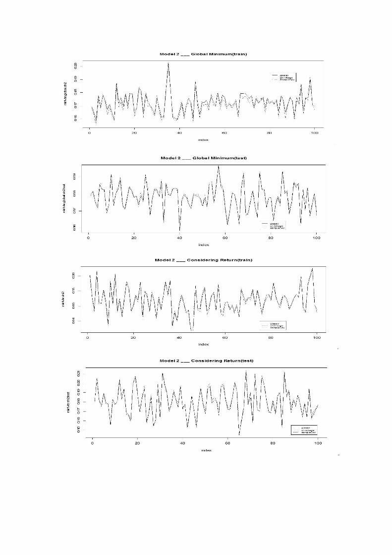
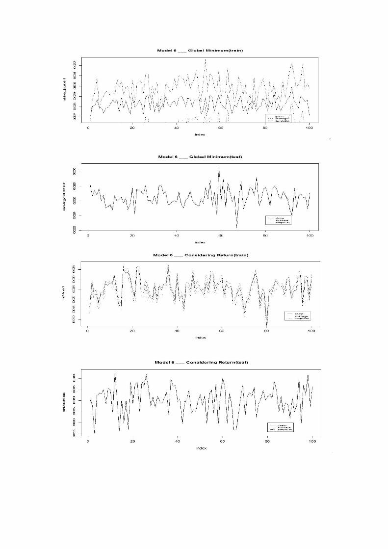
As shown in Figure 1-4, these are comparison of optimization result for Model 31.

The sample covariance gets the best performance in the train dataset of both the two

optimization while the Glasso estimator gets the best performance in the test dataset.

This is actually a desirable result since the goodness of the estimated covariance

matrix should be judged by how it performs to get a portfolio weight structure that

can gain more than others when applied to future data. What’s more, it is reasonable

to find that the sample covariance performs the best in the train data because the

sample covariance is the true covariance matrix for the train data.

1Figures for other models can be found in the appendixes

Figure 1

Figure 2

Figure 3

Figure 4

To see the significance that the Glasso performs better than the other estimators in

test data, we use t-test to exam the portfolio optimization result of Glasso estimator

compared with the other two estimator separately. The t-test’s null hypothesis is that

the optimized result of Glasso equals to that of sample covariance and shrinkage

estimator. And the alternative hypothesis is that the result of Glasso is smaller than the

others. As shown in Table 1, Glasso’s advantage over the other two estimators is most

significant in Model 3,4 and 8. Another important fact we should notice in the table is

that sample covariance is not significantly worse than Glasso only in model 7 which is

the full model where element variables is highly correlated with each other. This

corresponds with the theory that Glasso performs better in data with a sparse precision

matrix.

Global minimum variance Optimization considering return

Sample

covariance

Shrinkage

estimator

Sample

covariance

Shrinkage

estimator

Model 1 7.529993e-16 1 2.190922e-08 1

Model 2 2.101272e-25 0.3208471 9.987082e-22 0.2344433

Model 3 1.001844e-22 5.520879e-17 6.237072e-09 0.02483197

Model 4 7.915417e-19 7.118669e-08 1.788595e-12 0.01158764

Model 5 8.280318e-21 0.6967956 1.226117e-06 0.9867212

Model 6 6.868502e-16 0.05461308 1.04845e-05 0.9993311

Model 7 0.9766911 3.561808e-06 0.4037951 8.45485e-05

Model 8 1.891239e-24 5.771165e-24 2.622082e-10 2.007245e-05

Table 1. p-value of t-test

IV. Real World Examples

We consider two simple real world datasets. The component stocks return of DJI

and NASDAQ 100. The first datasets contains 30 component stocks and the second

datasets contains 85 component stocks2. We choose the daily data from 2010 to 2012

as the train data and that from 2013 as the test data. So there are 754 samples in the

train data and 252 samples in the test data. We use the holding period return because it

is assumed to approximately follow a normal distribution and is more stable than the

stock price. The HPR contains the dividend which also reduces the large jumping in

the data. To choose the tuning parameterλwhen using Glasso, we use BIC as the

criterion here in the real data due to the unavailability of true covariance matrix.

However, just apply Glasso to sample covariance of the return might not work

well. Because the precision matrix of the return is not necessarily sparse. We might

assume that the residual of the return using a factor model should have a sparse

precision matrix. So we apply the Fama-French model to the stock return and estimate

the covariance matrix separately. All component stocks are affected by the

Fama-French model. So the covariance between them can be partly explained by FF

model. The remaining part comes from the internal relationships between themselves.

In order to optimize the portfolio while the Fama-French factor keeps fluctuating, we

need to separate these two correlations.

2 The actual amount of components of NASDAQ 100 is 103. Here we filtered the some of the stocks due to the unavailability of data in the time periods we choose to study.

X𝑖 = 𝛽𝑖𝐹 + 𝜀𝑖,

cov(X) = 𝑐𝑜𝑣(𝑋1, 𝑋2, … , 𝑋𝑛),

𝑐𝑜𝑣(𝑋𝑖 , 𝑋𝑗) = 𝑐𝑜𝑣(𝛽𝑖𝐹 + 𝜀𝑖 , 𝛽𝑗𝐹 + 𝜀𝑗) = 𝑐𝑜𝑣(𝛽𝑖𝐹, 𝛽𝑗𝐹) + 𝑐𝑜𝑣(𝜀𝑖 , 𝜀𝑗)

Xi is the HPR of each component stocks, F is the four Fama-French model factors

and εi is the residual. We use the Fama-French model to separate the original data

into two parts, the Fama-French factor model data and the cleaned data. Then we use

the three methods to estimate the covariance matrix of the two parts separately and

add them up to get the estimated covariance matrix of the original data. This is

theoretical supported because the factor and residual is assumed to be independent in

the linear regression model.

Sample

Covariance

Glasso

Estimate

Shrinkage

Estimate

Global minimum variance (train) 3.89 x 10-05 1.37 x 10-05 4.2 x 10-05

Global minimum variance (test) 5.20 x 10-05 3.91 x10-05 5.08 x 10-05

Minimum objective considering return

(train)

-5.07 x 10-03 -1.89 x 10-03 -5 x 10-03

Minimum variance(train) 4.78 x 10-03 6.46 x 10-04 4.65 x 10-03

Minimum objective considering return

(test)

9.08 x 10-03 8.73 x 10-04 8.47 x 10-03

Minimum variance(test) 4.68 x 10-03 3.72 x 10-04 4.45 x 10-03

Return -4.39 x 10-03 1.25 x 10-03 -4.02 x 10-03

Table 2. DJI_independent model

Sample

Covariance

Glasso

Estimate

Shrinkage

Estimate

Global minimum variance (train) 3.89 x 10 -05 2.11 x 10 -05 3.99 x 10 -05

Global minimum variance (test) 5.20 x 10 -05 3.69 x 10 -05 5.05 x 10 -05

Minimum objective considering return

(train)

3.89 x 10 -05 2.11 x 10 -05 3.99 x 10 -05

Minimum variance(train) 3.89 x 10 -05 7.18 x 10 -05 3.92 x 10 -05

Minimum objective considering return

(test)

-4.96 x 10 -04 -9.56 x 10 -04 -5.02 x 10 -04

Minimum variance(test) 5.20 x 10 -05 3.69 x 10 -05 5.06 x 10 -05

Return(test) 5.48 x 10-04 9.94 x 10-04 5.53 x 10-04

Table 3. DIJ_Fama-French mode

Sample

Covariance

Glasso

Estimate

Shrinkage

Estimate

Global minimum variance (train) 8.20 x 10-05 2.19 x 10-05 9.2 x 10-05

Global minimum variance (test) 7.33 x 10-05 6.58 x10-05 7.34 x 10-05

Minimum objective considering return -8.59 x 10-03 -3.69 x 10-03 -8.61 x 10-03

(train)

Minimum variance(train) 8.23 x 10-03 1.74 x 10-03 8.31 x 10-03

Minimum objective considering return

(test)

1.68 x 10-02 2.46 x 10-03 1.67 x 10-02

Minimum variance(test) 6.85 x 10-03 1.24 x 10-03 6.83 x 10-03

Return -9.98 x 10-03 -1.22 x 10-03 -9.90 x 10-03

Table 4. NASDAQ_independent model

Sample

Covariance

Glasso

Estimate

Shrinkage

Estimate

Global minimum variance (train) 8.20 x 10 -05 24.99 x 10 -05 8.84 x 10 -05

Global minimum variance (test) 7.33 x 10 -05 5.98 x 10 -05 7.16 x 10 -05

Minimum objective considering return

(train)

8.20 x 10 -05 4.99 x 10 -05 8.84 x 10 -05

Minimum variance(train) 8.08 x 10 -03 1.72 x 10 -03 4.05 x 10 -03

Minimum objective considering return

(test)

-1.25 x 10 -05 -1.18 x 10 -05 -1.17 x 10 -05

Minimum variance(test) 7.33 x 10 -05 5.98 x 10 -05 7.16 x 10 -05

Return(test) 1.33 x 10-03 1.25 x 10-03 1.25 x 10-03

Table 5. NASDAQ_Fama-French model

As shown in the Table 2-5, using the Glasso estimator, we get the best

portfolio with the smallest variance and the largest return in the test data of both DJI

and NASDAQ component stock returns. What’s more, we get even smaller variance

in the Fama-French model compared with the independent model. For DJI, the

optimal portfolio with Fama-French model has a variance of 3.69 x 10 -05, which is

10 times smaller than that with the independent model 3.72 x 10-04. For NASDAQ,

the improvement is more significant, the variance is reduced from 1.24 x 10-03 to

5.98 x 10 -05 while the return is also increased.

V. Conclusion

Through the simulation and real data application above, we find that Graphical

LASSO performs well in the application to the portfolio optimization. And using a

factor model like Fama-French model can improve the result of portfolio optimization

significantly. Therefore, it is a useful and practical method to apply in practice to get

the estimate of stock return’s covariance matrix and do the optimization.

VI. Problems and Future plan

When applying Glasso to real data using Fama-French model in this paper, we

estimate 𝑋 − 𝛽𝐹 directly. This may cause a problem of getting a not positive definite

estimate. What’s more, just adding the two estimated covariance matrix up does not

utilize the significance of Glasso, that is estimating a sparse precision matrix.

Therefore, we plan to redo the Fama-French model using Woodbury Formula,

Following the formula, the precision matrix of return should be

Σ−1 = (Σ0 + 𝛽Ψ𝛽𝑇)−1 = Σ0−1 − Σ0

−1𝛽(Ψ−1 + 𝛽𝑇Σ0−1𝛽)𝛽𝑇Σ0

−1

Ψ−1 is the precision matrix of Fama-French factors, Σ0−1 is the precision

matrix of the residual. In this way, we might expect a better estimate and

guarantee the estimated covariance matrix to be positive definite.

Reference

Yuan, M., and Lin, Y. (2007), “Model Selection and Estimation in the Gaussian Graphical Model,”

Biometrika, 94, 19–35. [893,897]

Banerjee, O., El Ghaoui, L. E., and D’Aspremont, A. (2008), “Model Selection Through Sparse

Maximum Likelihood Estimation for Multivariate Gaussian or Binary Data,” Journal of Machine

Learning Research, 9,485–516. [893,895]

Friedman, J., Hastie, T., and Tibshirani, R. (2007), “Sparse Inverse Covariance Estimation With the

Graphical Lasso,” Biostatistics, 9, 432–441. [893,895,897]

Meinshausen, N., and Bühlmann, P. (2006), “High-Dimensional Graphs and Variable Selection With

the Lasso,” The Annals of Statistics, 34, 1436–1462. [897,898]

Tibshirani, R. (1996), “Regression Shrinkage and Selection via the Lasso,” Journal of the Royal

Statistical Society, Ser. B, 58, 267–288. [893]

Daniela M. Witten, Jerome H. Friedman, and Noah Simon(2011), "New Insight and Faster

computations for the Graphical Lasso", Journal of Computational and Graphical Statistics, 892-900

Max A. Woodbury, Inverting modified matrices, Memorandum Rept. 42, Statistical Research Group,

Princeton University, Princeton, NJ, 1950, 4pp MR 38136

Max A. Woodbury, The Stability of Out-Input Matrices. Chicago, Ill., 1949. 5 pp. MR 32564

Appendix