application of grey-markov chain model in software ... · results than other models and has...

Journal of Computers Vol. 30 No. 3, 2019, pp. 14-27

doi:10.3966/199115992019063003002

14

Application of Grey-Markov Chain Model in Software

Reliability Prediction

Gul Jabeen1, 2*, Xi Yang1, Ping Luo1, Sabit Rahim2

1 Key Laboratory for Information System Security, School of Software, Tsinghua University, Beijing 100084, China

{jgl14, xi-yang, luop}@mails.tsinghua.edu.cn

2 Department of Computer Sciences, Karakoram International University, Gilgit Baltistan, Pakistan

[email protected]

Received 8 August 2017; Revised 1 January 2018; Accepted 1 March 2018

Abstract. A variety of software reliability growth models have been proposed to analyze the

reliability of software, such as stochastic process models, neural network models and grey

theory models. When dealing with the limited amount of failure data, researchers tend to seek

for non-stochastic approaches because stochastic models require large samples of data to

determine underlying distributions. However non-stochastic approaches fail to deal with more

fluctuating data sequences. In this paper, we have used Grey-Markov Chain Model (G-MCM)

and show the effectiveness of model in handling dynamic software reliability data. G-MCM

combines the advantages of both grey prediction model (GM(1,1) and Markov Chain Model.

GM (1,1) can robustly deal with incomplete and imperfect information and gives excellent

prediction outcomes. At the same time, it takes the advantage of predictive power of Markov

chain which decreases the random variability of the data and zpositively effects the forecasting

accuracy. Musa’s failure datasets from various projects have been used to evaluate the

prediction capability of G-MCM and compared with GM (1, 1) and Modified Jelinski-Moranda

reliability prediction model. The comparison shows that the G-MCM has better prediction

results than other models and has adequate applicability in software reliability prediction

Keywords: GM (1,1), failures, Markov chain, software reliability prediction

1 Introduction

Software systems are comprised of various concepts such as specifications, test results, end-user

documentation, and maintenance records. These concepts are continuously playing a pivotal role in every

field of life in the contemporary era. Therefore, software reliability measurement becomes increasingly

important and its accurate prediction can help the software developers to make important decisions.

Although many software reliability prediction models were proposed but the unavailability of failure data

and complex nature of software systems make these reliability prediction models questionable.

Failure data have two basic problems such as data collecting during software development lifecycle

makes data limited and uncertain and failure occurrence is non-stationary process which generates

fluctuating data sequences. Data is always collected during the software development process, and failure

data which is most important for reliability analysis is collected during early testing and debugging phase

[1]. Traditional software reliability prediction models usually need a significant amount of data for

parameter estimation and prediction. If the reliability analysis of software started at the later stage of the

software development, i.e., after testing phase, then the predicted results will be too late to incorporating

any changes in decisions. Reliability analysis is initiated in the early stage of software development to

overcome this problem, but unavailability or a small sample of failure data generates inaccurate results.

To solve the above problem, Grey model GM (1,1) is considered suitable for forecasting software

reliability because it is specially designed to deal with uncertainty in data, i.e., having small samples and

* Corresponding Author

Journal of Computers Vol. 30 No. 3, 2019

15

inadequate information [2]. However, GM (1, 1) fails in the situations where the data sequences change

more randomly. On the other hand, because of random occurrence of failures, it is not convincing to

select a single grey prediction model which can consider all the significant factors. Hence we know that

every prediction model is developed with the hope to gain prediction accuracy. Prediction accuracy will

be better if more factors are considered that relate to the system dynamics. So the combination of

forecasting values from to more forecasting methods is also effective, because it is often superior to any

model alone. Therefore, the Markov chain will be a good choice to combine with the GM (1,1) model.

In this paper, a Markov chain which is based on statistical methods is integrated with the GM (1,1) to

enhance the prediction accuracy and extend the application scope of Grey prediction model. The

proposed model combines GM (1,1) prediction model with Markov chain is named as Grey Markov

Chain in Model (G-MCM). Moreover, the two famous Musa software failure datasets [3] are used to

analyze the effectiveness of G-MCM. G-MCM proved to be deal well with both the fluctuating

sequences and limited amount of failure data sequences. The experimental results show that the proposed

G-MCM has proved to be more efficient prediction model with dynamic software reliability data.

Furthermore, G-MCM prediction is compared with two famous reliability prediction models, i.e.,

statistical modified-JM prediction model [4] and GM(1,1) to show its applicability. This comparison will

help the developers to choose the most suitable method for software reliability prediction.

The remainder of this paper is organized as follows. In section 2, we have introduced the detailed

related work. Section 3 describes grey system theory, which includes grey prediction model GM (1,1) in

detail. Section 4 introduces the G-MCM model, which combines the GM (1,1) with the Markov Chain

model. In section 5 application of G-MCM model on software failure dataset has been presented. Section

6 shows the comparison between predictive values of G-MCM and Modified J-M Model. Section 7

illustrates the result evaluation of G-MCM model. Section 8 concludes the paper.

2 Literature Review

The software reliability estimation is a long existed problem in software engineering field. It is still a

progressing field, although tremendous theoretical and empirical software reliability models have been

developed. These models are divided into two main categories such as stochastic and non-stochastic

process models.

Stochastic process models are important and widely used software reliability predictive models, which

consider failure interval as an exponentially distributed stochastic process. Jelinski and Moranda [4]

proposed a basic software reliability growth model called Jelinski-Moranda (J-M) model based on

Markov process, which laid the basic foundation of software reliability measurement. Musa [3]

developed the basic execution time model with the similar assumptions as J-M model with some

significant modifications. Mahapatra and Roy [5] introduced a Modified-Jelinskie-Morenda (M-J-M)

model using imperfect debugging process in fault removal activity. Another type of stochastic reliability

prediction models is Non Homogenous Poisson Process (NHPP) model which consider software failure

interval as Poisson distribution. Geol and Okumoto [6] developed the first NHPP model with the

assumption of the fault removal process follows NHPP. Zhao et al. poposed a software reliability growth

model from testing to operation which incorporates environmental function and inherent fault detection

rate based on NHPP. Chatterjee and Singh [7], Kundu et al. [8] and Li and Pham [9] also proposed more

advanced and optimized models based on NHPP models. However, the performance of all the above

stochastic models depends on the failure sample size.

Similarly, in recent years, researchers try to use some non-stochastic process models for software

reliability estimation. The Artificial intelligence algorithms are most commonly used models. Cai et al.

[10], Aggarwal and Gupta [11], Lakshmanan and Ramasamy [12] and Bhuyan and Mohapatra [13]

applied neural network methods which are used to estimate the number of software defects, categorize

program modules, and predict the number of detected software failures and produced better results. In the

same line, Costa et al. [14], Kim and Baik [15] estimate software reliability by using genetic algorithms

and provide a comprehensive optimal solution to avoid local minimum problems, but their

implementation is very complicated. Recently, grey system theory is applied in every field of life, such as

agriculture, industries, health and technology [16-18]. Among all grey models, the GM (1,1) is the most

widely used technique and the basic prediction framework based on grey theory. Mei [19] and Mao [20]

proposed the basic fault prediction model based on GM (1,1). These models deal with the fault data

Application of Grey-Markov Chain Model in Software Reliability Prediction

16

recorded in software maintenance stage where the sample size is very small and the grey modeling

provides better results.

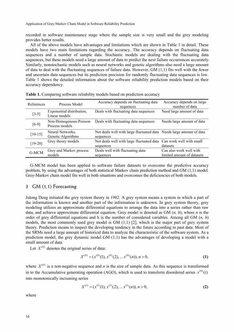
All of the above models have advantages and limitations which are shown in Table 1 in detail. These

models have two main limitations regarding the accuracy. The accuracy depends on fluctuating data

sequences and a number of sample data. Stochastic models are dealing with the fluctuating data

sequences, but these models need a large amount of data to predict the next failure occurrences accurately.

Similarly, nonstochastic models such as neural networks and genetic algorithms also need a large amount

of data to deal with the fluctuating sequences of failure data. However, GM (1,1) fits well with the fewer

and uncertain data sequences but its prediction precision for randomly fluctuating data sequences is low.

Table 1 shows the detailed information about the software reliability prediction models based on their

accuracy dependency.

Table 1. Comparing software reliability models based on prediction accuracy

References Process Model Accuracy depends on fluctuating data

sequences

Accuracy depends on large

number of data

[3-5] Exponential distribution,

Linear models

Deals with fluctuating data sequences Need large amount of data

[6-9] Non-Homogenous-Poisson

Process models

Deals with fluctuating data sequences Needs large amount of data

[10-15] Neural Networks,

Genetic Algorithms

Not deals well with large fluctuated data

sequences

Needs large amount of data

[19-20] Grey theory models Not deals well with large fluctuated data

sequences

Can work well with small

datasets

G-MCM Grey and Markov process

models

Deals well with fluctuating data

sequences

Can also work well with

limited amount of datasets

G-MCM model has been applied to software failure datasets to overcome the predictive accuracy

problem, by using the advantages of both statistical Markov chain prediction method and GM (1,1) model.

Grey-Markov chain model fits well in both situations and overcomes the deficiencies of both models.

3 GM (1,1) Forecasting

Julong Deng initiated the grey system theory in 1982. A grey system means a system in which a part of

the information is known and another part of the information is unknown. In grey system theory, grey

modeling utilizes an approximate differential equations to arrange the data into a series rather than raw

data, and achieve approximate differential equation. Grey model is denoted as GM (n, h), where n is the

order of grey differential equations and h is the number of considered variables. Among all GM (n, h)

models, the most commonly used grey model is GM (1,1) [2], which is the major part of grey system

theory. Prediction means to inspect the developing tendency in the future according to past data. Most of

the SRMs need a large amount of historical data to analyze the characteristic of the software system. As a

prediction model, the grey dynamic model GM (1,1) has the advantages of developing a model with a

small amount of data.

Let (0)X denotes the original series of data:

(0) (0) (0) (0)( (1), (2), ... ( )), 0,X x x x n n= > (1)

where (0)X is a non-negative sequence and n is the size of sample data. As this sequence is transformed

in to the Accumulative generating operation (AGO), which is used to transform disordered series (0) ( )x i

into monotonically increasing series

(1) (1) (1) (1)( (1), (2), ... ( )), 0,X x x x n n= > (2)

where


17

(1) (0)

1

( ) ( ), 1, 2, 3 ..., .j

i

x t x i j n=

= =∑ (3)

It is clear that the original data (0) ( )x i can be easily recovered, from (1) ( )x i as

(0) (1) (0)( ) ( ) ( 1).x i x i x i= − − . (4)

Based on the (1)X , we can get its mean sequence as follows:

(0) (1) (1) (1)( (2), (3), ... ( )),Z z z z n= (5)

where (1) ( )z t is the mean value of adjacent data, i.e.

(1) (1) (1)( ) 0.5 ( ) 0.5 ( 1),Z t x t x t= + − k=2, 3, ..., n (6)

The least square estimate sequence of the first order grey differential equation is defined as follows:

(0) (1)( ) ( ) .x t az t b+ = (7)

Where “a” is called the development coefficient and “b” is called driving coefficients. By using the

least square method, the estimation coefficient can be estimated.

(1) (0)

(1) (0)

(1) (1)

(2) 1 (2)

(3) 1 (3), , .

( ) 1 ( )

z x

z x aA Y

b

z n x n

β

⎡ ⎤ ⎡ ⎤−⎢ ⎥ ⎢ ⎥− ⎡ ⎤⎢ ⎥ ⎢ ⎥

= = = ⎢ ⎥⎢ ⎥ ⎢ ⎥⎣ ⎦⎢ ⎥ ⎢ ⎥

⎢ ⎥ ⎢ ⎥−⎣ ⎦ ⎣ ⎦

� � � � (8)

Based on the principle of least square method, we have

( ) ,T TA A A Yβ = , (9)

Hence, by using coefficient “a” and “b” we can construct the following response equation for future

prediction:

(1) (0)( 1) ( (1) ) .akb bx k x e

a a

−

+ = − + (10)

Thus the simulated value of (0)X can be obtained by using following equation:

(0) (1) (1)( 1) ( 1) ( ).x k x k x k+ = + − . (11)

It is commonly believed that the differential equation is only appropriate for continuous differential

function. The GM (1,1) with the differential equation is established based on discrete data with a

minimum number of samples.

4 G-MCM Reliability Prediction Model Understanding

Software failure data is more fluctuating and has a significant number of uncertainties. The predictive

accuracy of GM (1,1) is not appropriate because of its randomness, so Markov chain model is used to

enhance the prediction accuracy of GM (1,1) model. Thus, the G-MCM model is a combination of two

models such as GM (1,1) and Markov chain. The basic idea is to model the original data by using GM

(1,1) and obtain the residual errors from it. Subsequently, these error sequences are divided into different

states based on the historical data and find the central values. Then the Markov chain is used to establish

the transition behavior between different states by using Markov transition matrices, then conceivable

improvement for the predictive value can be made. The further detailed procedure is shown in [21]. The

following section shows the different steps to develop G-MCM reliability prediction model.


18

4.1 Division of States

Based on the original sequence of failure data (0) ( )x i , the predicted values of obtained by using GM(1, 1)

such as (0)ˆ ( )x i . After getting estimated values the residual errors (0) (0)ˆ( ) ( ) ( )e i x i x i= − can be obtained.

The residual errors divided into n states and each state zone is as follows

,

[ ], 1, 2 , .ij ij ijL U j n⊗ = = … (12)

Hence, ij⊗ is the j-th state of i-th timestamp having an interval whose width is fixed portion of the

range between the lower ijL and upper ijU limit of the whole residual error. Based on the historical data,

the numbers of states are decided, more historical data should be divided into more states and less

historical data cause fewer states.

4.2 Compute Central Values

According to the number of states as defined in equation 12 their central value are calculated. In this

model, mean is considering as a central value for different states such as

2

ij in

nv

⊗ + ⊗=

�

(13)

Hence, nv will be constant and used to predict next value.

4.3 Compute State Transition Probability Matrix

If the residual errors are divided into n-th states, then there will be n transition probability rows vectors.

Assume that the state n-th step transition probability is calculated using the following formula:

, 1, 2, 3 ..., .

n

ijn

ij

i

NP j n

N= = (14)

We specify that n

ijP is the probability transition from i-th state to the j-th state by n-th steps. Hence n

ijN

is the transition time of i-th state to j-th states by n steps and i

N is the total number of specified states.

( ) ( ) ( )11 12 1

( ) ( ) ( )21 22 2( ) ,

n n n

n

n n n

n

p p p

P n p p p

⎡ ⎤⎢ ⎥

= ⎢ ⎥⎢ ⎥⎣ ⎦

�

�

� � � �

(15)

It should satisfy the following properties

( )

1

1.n

ij

j

p

=

=∑

4.4 Compute Predicted Value

Although the last transition state is not known and the possibility of next state is predicted by using the

state transition matrix and n-th row vector, which is represented as ( ),ia k where 1, 2 , ,i n= … in k-th

time step.

(0)ˆ ˆ( 1) ( 1) , 1, 2 , .i

y k x k v i n+ = + + = … (16)

The center of n states are represented as iv , where

1

( ) [ ( ), ... ( )] ( 1)* ( )n

a n a k a k a k P n= = − (17)


19

and the next probability states can be determined as follows:

( 1) ( ) ( )

( 2) ( 1) ( )

( 1) ( 1) ( )

a k a k P n

a k a k P n

a k a k l P n

+ =⎧⎪ + = +⎪⎨⎪⎪ + = + −⎩

�

where n=1.

5 Application of G-MCM Model for Musa Failure Datasets

In this section, authors have concentrated on the analysis of two sets of real software reliability dataset

published by Musa [3]. Among many software reliability models, J-M model is the classic model.

Therefore, we choose Modified J-M model for comparison. A comparison of G-MCM with the most

popular software reliability stochastic model M-J-M and GM (1, 1) was carried out. In all cases, the G-

MCM provided higher prediction results than others.

5.1 Analysis of Musa System on Failure Data

Based on the 131 Musa systems 1 failure dataset, GM (1, 1) and G-MCM models are analyzed. For G-

MCM model prediction, the original data series (0) (0) (0)ˆ ˆ ˆ{ (1), (2) ... ( )}x x x n are first modeled by the GM

(1, 1) prediction model, then the residual error series {{ (1), (2) ... ( )}e e e n between the actual values and

predicted values for all the previous time steps are recorded. By using the least square method using

equation 8, the parameters 0.021a = − and 113.226b = are computed.

According to the residual errors of 131 Musa dataset, the corresponding intervals are divided into five

states for our model analysis.

The five states listed below are determined by using equation 12:

1 2 3 4 5

[ 500], [ 500, 100], [ 100, 0], [0, 500], [ 500]⊗ = > − ⊗ = − − ⊗ = − ⊗ = ⊗ = >

According to the states defined above, we calculate their central value using equation 13:

1 2 3 4 5

972, 246.66, 45.1, 223.33, 1511,v v v v v= − = − = − = =

The model fitted and estimated values by GM (1, 1), and G-MCM prediction model are plotted in Fig.

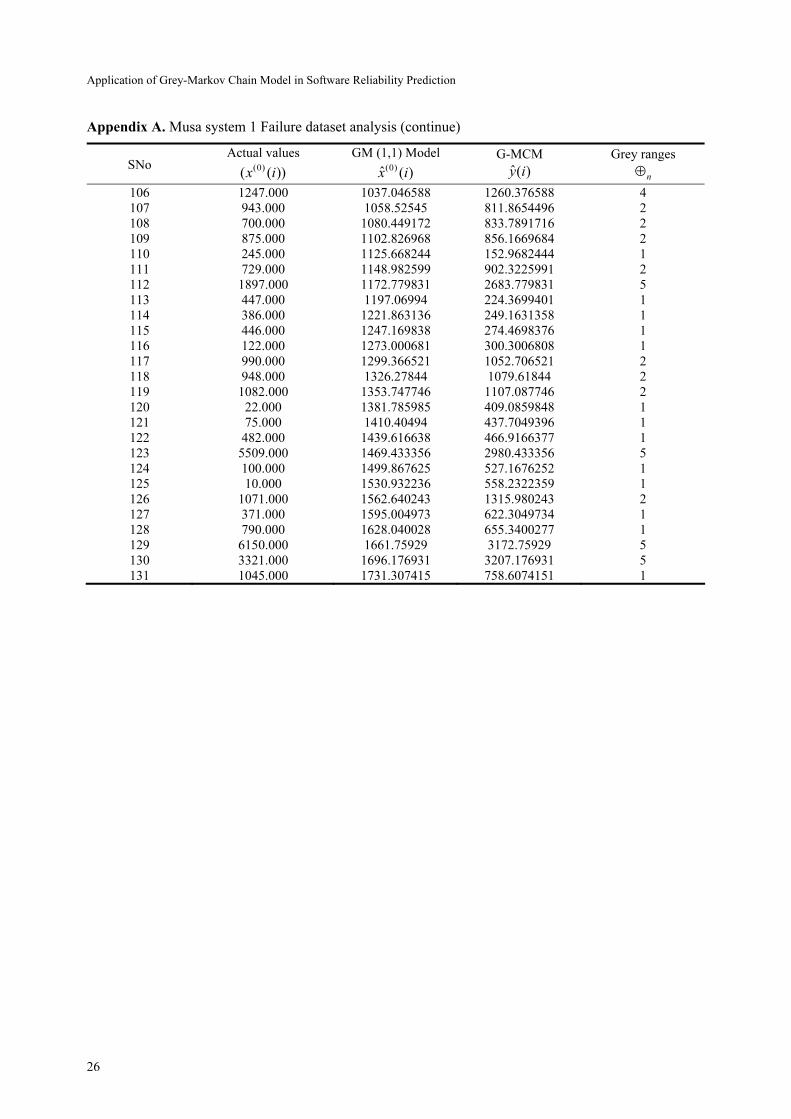
1 and Fig. 2. The detailed table is shown in Appendix A.

0

1000

2000

3000

4000

5000

6000

7000

1 6 11 16 21 26 31 36 41 46 51 56 61 66 71 76 81 86 91 96 101106111116121126131

Failure

Tim

e

Failure Number

Actual values

GM(1,1)

0

1000

2000

3000

4000

5000

6000

7000

1 6 11 16 21 26 31 36 41 46 51 56 61 66 71 76 81 86 91 96 101106111116121126131

Failure

Tim

e

Failure Number

Actual values

GMCM

Fig. 1. Actual versus GM (1, 1) predicted values Fig. 2. Actual versus G-MCM predicted values

Fig. 1 shows that the GM (1,1) gives an exponential curve that is smooth and it does not counterpart

with the data, which has high changing sequences because its forecast accuracy is low. Fig. 2 shows the


20

G-MCM prediction model fitted data and it shows clearly that the predicted values are accurate with both

high changing and low changing sequences.

5.1.1 Calculating Predicted Values

The transition probability matrix ( )P n for 131-datasets can be calculated according to the method

described above.

0.5789 0.1578 0.0000 0.0526 0.2105

0.0625 0.4791 0.2708 0.1254 0.1578

( ) 0.0357 0.4285 0.2857 0.1071 0.2105

0.0526 0.4736 0.2105 0.1578 0.1052

0.2500 0.0625 0.1250 0.3750 0.1578

P n

⎡ ⎤⎢ ⎥⎢ ⎥⎢ ⎥=⎢ ⎥⎢ ⎥⎢ ⎥⎣ ⎦

The 131-th row vector used to obtain the next state (131) [0.5789 0.1578 0.0000 0.0526 0.2105]a =

Based on the Markov chain model results the next state a(132) is 1, so the residual error for 132-th failure

data is in the state 1

[ 500].⊗ = > − According to the predicted state 1, we can calculate the central value as

1972.7,v = − where (0)ˆ (132) 1731.30x = is the predicted value of GM (1, 1) model. The G-MCM

predicted value ˆ( )y i is obtained using equation 16.

ˆ(132) 1731.30 ( 972.7)

ˆ(132) 794.47

y

y

= + −

=

As the original value of 132-th failure is 648 and the predicted value by using G-MCM model is

794.47, which is very close to actual data.

5.2 Analysis of Musa system 3 Failure Data

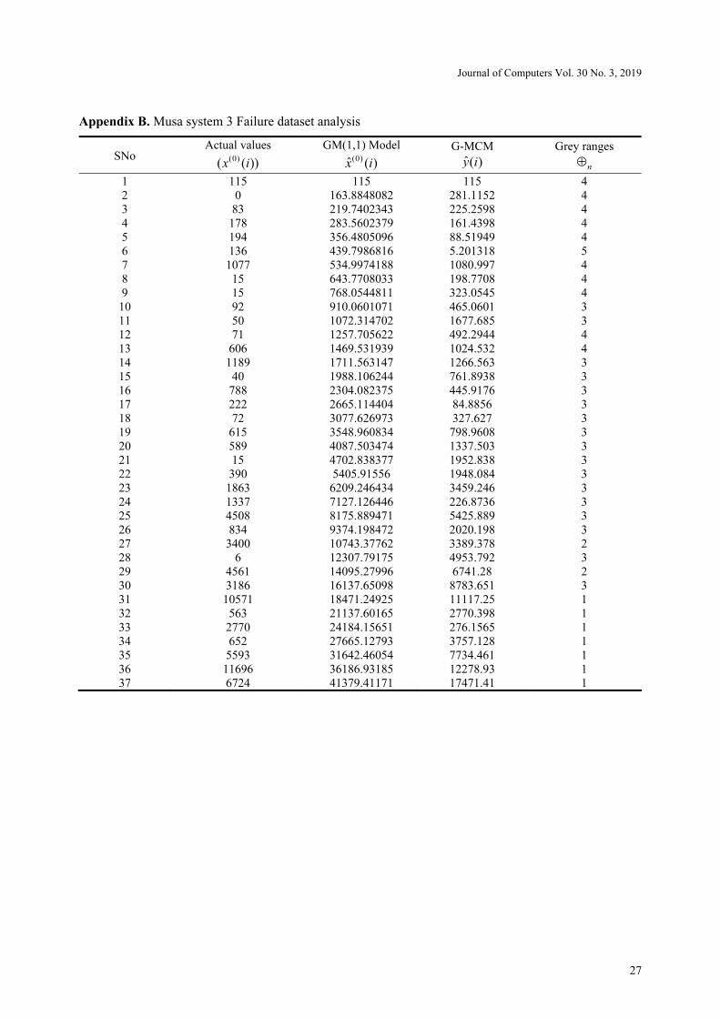
Similarly, 36 Musa system 3 failure datasets are used to evaluate G-MCM model. The computed

parameters by using equation (8) are 0.133a = − and 30.369.b = According to the predicted data series

by GM (1, 1) model we can obtain its residual errors. From the obtained residual errors, the

corresponding intervals are divided in to five states based on the equation 12:

1 2 3 4 5

[ 2000], [ 20000, 5000], [ 5000, 1000], [ 1000, 0], [ 0]⊗ = > − ⊗ = − − ⊗ = − − ⊗ = − ⊗ = >

Based on the above five states the central values are calculated as follows:

1 2 3 4 5

23908, 7354, 2750, 445.8, 546v v v v v= − = − = − = − =

The GM (1,1) and G-MCM model predicted values by using Musa system 3 failure dataset are plotted

in Fig. 3 and Fig. 4. Appendix B shows the detailed information.

0

5000

10000

15000

20000

25000

30000

35000

40000

1 2 3 4 5 6 7 8 9 10 1112 1314 15 16 17 18 19 2021 2223 24 25 26 27 28 2930 3132 33 34 35 36

Failure

Tim

e

Failure Number

Actual values

GM(1,1)

0

2000

4000

6000

8000

10000

12000

14000

1 2 3 4 5 6 7 8 9 10 11 12 13 14 15 16 17 18 19 20 21 22 23 24 25 26 27 28 29 30 31 32 33 34 35 36

Failure

Tim

e

Failure Number

Actual values

GMCM

Fig. 3. Actual versus GM (1,1) predicted values Fig. 4. Actual versus G-MCM predicted values


21

In Fig. 3 the GM (1,1) model shows the exponential curve that is smooth and it does not counterpart

with the data, which has fluctuating sequences. Fig. 4 shows the best accuracy of predicted values of G-

MCM model with both high and low changing sequences.

5.2.1 Calculating Predicted Values

Base on the Markov Chain prediction the transition probability matrix ( )P n for 36 datasets can be

calculated according to the method described above.

1.000 0.000 0.000 0.000 0.000

0.000 0.000 1.000 0.000 0.000

( ) 0.0588 0.117 0.764 0.058 0.000

0.000 0.000 0.200 0.700 0.100

0.000 0.000 0.000 1.000 0.000

P n

⎡ ⎤⎢ ⎥⎢ ⎥⎢ ⎥=⎢ ⎥⎢ ⎥⎢ ⎥⎣ ⎦

The 36-th row vector is:

(36) [1 0 0 0 0]a =

Based on equation (12) the 37-th predicted error state is 1 such as 1

20000.⊗ => − The calculated

central value for state 1 is 23908,iv = − and the predicted value of GM(1,1) model is

(0) (36) 36186.x =

Based on the obtained central value and GM(1,1) predicted value the G-MCM predicted value ˆ( )y i is

obtained using equation (16):

ˆ(37) 41379 ( 23908)

ˆ(37) 17471

y

y

= + −

=

For instance, the original value of 37-th failure is 6724 and the predicted value by G-MCM model is

17471, which is more close to the actual data.

6 Comparison between the Predicted Values of G-MCM and M-J-M Model

Based on the two Musa-failure datasets as described above, a comparison between G-MCM and M-J-M

reliability prediction model is made. For instance, the models fitted and the original Musa experimental

data are shown in Fig. 5 and Fig. 6.

0

1000

2000

3000

4000

5000

6000

7000

1 6 11 16 21 26 31 36 41 46 51 56 61 66 71 76 81 86 91 96 101106111116121126131

Failure

Tim

e

Failure Number

Actual values

M-JM

GMCM

0

2000

4000

6000

8000

10000

12000

14000

16000

1 2 3 4 5 6 7 8 9 10 11 12 13 14 15 16 17 18 19 20 21 22 23 24 25 26 27 28 29 30 31 32 33 34 35 36

Failure

Tim

e

Failure Number

Actual values

M-JM

GMCM

Fig. 5. Actual Musa 3 dataset versus J-M and

G-MCM

Fig. 6. Actual Musa 1 dataset versus J-M and

G-MCM


22

Meanwhile, Fig. 5 and Fig. 6, show the relationship of actual failure time with the traditional statistical

model M-J-M and G-MCM, which is clear indication of the failure prediction behavior of the models.

The figures show clearly that the predicted results of G-MCM are more accurate than M-J-M model.

Furthermore, authors have also discussed more clear evaluation criterion, which discusses the model’s

prediction accuracy results in more detail.

7 Results Evaluation

We used the evaluation criteria for each model to measure its performance and prediction capability.

Following are the three criteria of the evaluation method, which are used to compare different models

such as root mean square error (RMSE), mean absolute error (MAE) and average absolute error

percentage (AAEP). These are calculated as follows:

2

1 1 1

1 1 1( ) | | 100

n n n

i i

i i i i

ii i i

a pRMSE a p MAE a p AAEP

n n n a= = =

−

= − = − = ×∑ ∑ ∑　　　　

In statistics, the above evaluation criterion is used to measure how close the estimated or predicted

values ip with the actual outcomes

ia The forecast values of Musa failure 1 and 3 datasets are calculated

by Modified J-M, GM (1,1) and G-MCM models. Based on these forecasted values the models were

compared, results are analyzed based on the above evaluation criterion shown in Table 2.

Table 2. A comparison of prediction results between three models

Musa System 1 Failure Data Musa System 3 Failure Data

M-J-M Model GM(1,1) Model G-MCM Model M-J-M Model GM(1,1) Model G-MCM Model

RMSE 872.86 795.40 422.06 3901 11449 2432.6

MAE 577.0 461.72 185.09 3014 6995.4 1333.6

AAEP 964.7 669.80 210.22 5435 7666.7 2996.2

As the GM (1, 1) model is elementary to use and require few calculations, but its accuracy is not

satisfactory when the data is more fluctuating or having high randomness. The evaluation matrices in

Table 2 shows that GM (1, 1) prediction accuracy is not good with every failure data set, but when it is

combined with Markov Chain the results become more satisfying and gives more accurate prediction

results. As the predicted values in section 5.1.1 and 5.2.1 also show good results then M-J-M and GM (1,

1) models. However, Table 2 shows that the G-MCM prediction model is better for the software

reliability prediction and the forecast values of the G-MCM are more precise and accurate than M-J-M

and GM (1, 1) model.

8 Conclusion

The main purpose of this model was to show the applicability of G-MCM prediction model for software

reliability prediction. Through using different failure datasets, we have proved the effectiveness of G-

MCM model. The combined effect GM (1,1) and Markov chain achieved more accurate results than

other conventional models and the predicted values are also close to the actual values. This model is not

only considered suitable for predicting fluctuating data sequences, but can also be applied to early

software reliability prediction with less amount of data. Therefore, this model is considered suitable for

the prediction of the more dynamic system such as the failure variability of software systems having less

amount of data. Hence, the prediction accuracy is associated with the number of states. There is no

standard to resolve the problem of state division. Therefore, the model needs further enhancements and

review.

References

[1] R.M. Lyu, Handbook of Software Reliability Engineering, McGraw-Hill, New York, 1996.


23

[2] S. Liu, Y. Lin, Grey System Theory and Application, Springer-Verlag, Berlin, 2011.

[3] J. Musa, Data analysis center for software: an information analysis center, [dissertation] Kalamazoo, MI: Western Michigan

University, 1979.

[4] Z. Jelinski, P. Moranda, Software Reliability Research, Academic Press, New York, 1972.

[5] G. Mahapatra, P. Roy, Modified Jelinski-Moranda software reliability model with imperfect debugging phenomenon,

International Journal of Computer Applications 48(18)(2012) 38-46.

[6] A.L. Goel, K. Okumoto, Time-dependent error-detection rate model for software reliability and other performance measures,

IEEE Transactions on Reliability R-28(3)(1979) 206-211.

[7] S. Chatterjee, J.B. Singh, A NHPP based software reliability model and optimal release policy with logistic-exponential test

coverage under imperfect debugging, International Journal of Systems Assurance Engineering and Management 5(3)(2014)

399-406.

[8] S. Kundu, T.K. Nayak, S. Bose, Are nonhomogeneous poisson process models preferable to general-order statistics models

for software reliability estimation? in: F.Vonta, M. Nikulin, N. Limnios, C. Huber-Carol (Eds.), Statistical Models and

Methods for Biomedical and Technical Systems, Birkhäuser Boston, Boston, 2008, pp. 137-152.

[9] Q. Li, H. Pham NHPP software reliability model considering the uncertainty of operating environments with imperfect

debugging and testing coverage, Applied Mathematical Modelling 51(2017) 68-85.

[10] K.-Y. Cai, L. Cai, W.-D. Wang, Z.-Y. Yu, D. Zhang, On the neural network approach in software reliability modeling,

Journal of Systems and Software 58(1)(2001) 47-62.

[11] G. Aggarwal, V.K. Gupta, Neural network approach to measure reliability of software modules: a review, International

Journal of Advances in Engineering Sciences 3(2)(2013) 1-7.

[12] I. Lakshmanan, S. Ramasamy, An artificial neural-network approach to software reliability growth modeling, Procedia

Computer Science 57(2015) 695-702.

[13] M.K. Bhuyan, D.P. Mohapatra, Prediction strategy for software reliability based on recurrent neural network,

Computational Intelligence in Data Mining 411(2016) 295-303.

[14] E.O. Costa, S.R. Vergilio, A. Pozo, G. Souza, Modeling software eeliability growth with genetic programming, in: Proc.

16th IEEE International Symposium on Software Reliability Engineering (ISSRE’05), 2005.

[15] T. Kim, K. Lee, J. Baik, An effective approach to estimating the parameters of software reliability growth models using a

real-valued genetic algorithm, Journal of Systems and Software 102(2015) 134-144.

[16] E. Kayacan, B. Ulutas, O. Kaynak, Grey system theory-based models in time series prediction, Expert Systems with

Applications 37(2)(2010) 1784-1789.

[17] X. Wang, L. Qi, C. Chen, J. Tang, M. Jiang, Grey system theory based prediction for topic trend on Internet, Engineering

Applications of Artificial Intelligence 29(2014) 191-200.

[18] L. Li, R. Wang, X. Li Grey, GM (1, 1, βk) Model and its Application in R & D Personnel, Journal of Grey System

29(1)(2017) 120-134.

[19] D. Mei, Novel model of software reliability by the grey system theory, in: Proc. 2007 IEEE International Conference on

Electro/Information Technology, 2007.

[20] C. Mao, Software faults prediction based on grey system theory, SIGSOFT Software Engineering Notes 34(2)(2009) 1-6.

[21] G. Li, D. Yamaguchi, M. Nagai, A GM (1,1) – Markov chain combined model with an application to predict the number of

Chinese international airlines, Technological Forecasting and Social Change 74(8)(2007) 1465-1481.


24

Appendix

Appendix A. Musa system 1 Failure dataset analysis

SNo Actual values

(0)( ( ))x i

GM (1,1) Model (0)ˆ ( )x i

G-MCM

ˆ( )y i

Grey ranges

n⊕

1 3.000 3 3 3

2 30.000 122.9935769 77.89357686 3

3 113.000 125.5409667 80.44096672 3

4 81.000 128.141117 83.04111702 3

5 115.000 130.7951205 85.69512051 3

6 9.000 133.5040926 113.1559074 2

7 2.000 136.2691717 110.3908283 2

8 91.000 139.0915199 93.99151994 3

9 112.000 141.9723234 96.87232345 3

10 15.000 144.9127929 101.7472071 2

11 138.000 147.9141641 102.8141641 3

12 50.000 150.9776984 95.68230158 2

13 77.000 154.1046833 109.0046833 3

14 24.000 157.296433 89.36356701 2

15 108.000 160.5542888 115.4542888 3

16 88.000 163.8796199 118.7796199 3

17 670.000 167.2738238 1678.273824 5

18 120.000 170.7383271 125.6383271 3

19 26.000 174.2745856 72.38541443 2

20 114.000 177.8840855 132.7840855 3

21 325.000 181.5683439 404.8983439 4

22 55.000 185.3289091 61.33109094 2

23 242.000 189.1673614 412.4973614 4

24 68.000 193.0853141 53.57468588 2

25 422.000 197.0844138 420.4144138 4

26 180.000 201.1663411 156.0663411 3

27 10.000 205.3328115 41.32718853 2

28 1146.000 209.585576 1720.585576 5

29 600.000 213.926422 437.256422 4

30 15.000 218.3571737 28.30282634 2

31 36.000 222.8796932 23.78030684 2

32 4.000 227.4958811 19.16411887 2

33 0.000 232.2076776 14.4523224 2

34 8.000 237.0170628 9.642937238 2

35 227.000 241.9260578 196.8260578 3

36 65.000 246.9367259 0.276725889 2

37 176.000 252.0511727 206.9511727 3

38 58.000 257.2715478 10.6115478 2

39 457.000 262.600045 485.930045 4

40 300.000 268.0389038 491.3689038 4

41 97.000 273.5904098 26.93040982 2

42 263.000 279.2568963 234.1568963 3

43 452.000 285.0407445 508.3707445 4

44 255.000 290.9443854 245.8443854 3

45 197.000 296.9702999 251.8702999 3

46 193.000 303.1210205 56.46102049 2

47 6.000 309.3991322 62.73913219 2

48 79.000 315.8072734 69.14727343 2

49 816.000 322.3481373 545.6781373 4

50 1351.000 329.0244728 1840.024473 5


25

Appendix A. Musa system 1 Failure dataset analysis (continue)

SNo Actual values

(0)( ( ))x i

GM (1,1) Model (0)ˆ ( )x i

G-MCM

ˆ( )y i

Grey ranges

n⊕

51 148.000 335.8390856 89.17908559 2

52 21.000 342.7948397 96.13483973 2

53 233.000 349.8946584 103.2346584 2

54 134.000 357.1415255 110.4815255 2

55 357.000 364.5384866 319.4384866 3

56 193.000 372.0886504 125.4286504 2

57 236.000 379.7951898 133.1351898 2

58 31.000 387.6613438 141.0013438 2

59 369.000 395.6904182 350.5904182 3

60 748.000 403.8857873 627.2157873 4

61 0.000 412.2508954 165.5908954 2

62 232.000 420.7892579 174.1292579 2

63 330.000 429.5044633 384.4044633 3

64 365.000 438.4001743 393.3001743 3

65 1222.000 447.4801295 402.3801295 5

66 543.000 456.7481447 680.0781447 4

67 10.000 466.2081151 219.5481151 2

68 16.000 475.8640163 229.2040163 2

69 429.000 485.7199063 440.6199063 3

70 379.000 495.7799273 249.1199273 2

71 44.000 506.0483071 259.3883071 2

72 129.000 516.5293612 269.8693612 2

73 810.000 527.2274943 750.5574943 4

74 290.000 538.1472025 291.4872025 2

75 300.000 549.293075 302.633075 2

76 529.000 560.669796 515.569796 3

77 281.000 572.2821468 325.6221468 2

78 160.000 584.1350075 337.4750075 2

79 828.000 596.2333596 819.5633596 4

80 1011.000 608.5822875 831.9122875 4

81 445.000 621.1869811 374.5269811 2

82 296.000 634.0527376 387.3927376 2

83 1755.000 647.1849642 2158.184964 5

84 1064.000 660.5891797 883.9191797 4

85 1783.000 674.2710176 2185.271018 5

86 860.000 688.2362278 911.5662278 4

87 983.000 702.4906794 925.8206794 4

88 707.000 717.040363 671.940363 3

89 33.000 731.8913934 240.8086066 1

90 868.000 747.050012 970.380012 4

91 724.000 762.5225893 717.4225893 3

92 2323.000 778.3156279 2289.315628 5

93 2930.000 794.4357652 2305.435765 5

94 1461.000 810.8897757 2321.889776 5

95 843.000 827.6845747 1051.014575 4

96 12.000 844.8272202 127.8727798 1

97 261.000 862.3249168 110.3750832 1

98 1800.000 880.1850182 2391.185018 5

99 865.000 898.4150303 853.3150303 3

100 1435.000 917.0226145 2428.022614 5

101 30.000 936.0155909 36.68440906 1

102 143.000 955.4019417 17.29805828 1

103 108.000 975.1898142 2.489814239 1

104 0.000 995.3875246 22.68752463 1

105 3110.000 1016.003561 2527.003561 5


26

Appendix A. Musa system 1 Failure dataset analysis (continue)

SNo Actual values

(0)( ( ))x i

GM (1,1) Model (0)ˆ ( )x i

G-MCM

ˆ( )y i

Grey ranges

n⊕

106 1247.000 1037.046588 1260.376588 4

107 943.000 1058.52545 811.8654496 2

108 700.000 1080.449172 833.7891716 2

109 875.000 1102.826968 856.1669684 2

110 245.000 1125.668244 152.9682444 1

111 729.000 1148.982599 902.3225991 2

112 1897.000 1172.779831 2683.779831 5

113 447.000 1197.06994 224.3699401 1

114 386.000 1221.863136 249.1631358 1

115 446.000 1247.169838 274.4698376 1

116 122.000 1273.000681 300.3006808 1

117 990.000 1299.366521 1052.706521 2

118 948.000 1326.27844 1079.61844 2

119 1082.000 1353.747746 1107.087746 2

120 22.000 1381.785985 409.0859848 1

121 75.000 1410.40494 437.7049396 1

122 482.000 1439.616638 466.9166377 1

123 5509.000 1469.433356 2980.433356 5

124 100.000 1499.867625 527.1676252 1

125 10.000 1530.932236 558.2322359 1

126 1071.000 1562.640243 1315.980243 2

127 371.000 1595.004973 622.3049734 1

128 790.000 1628.040028 655.3400277 1

129 6150.000 1661.75929 3172.75929 5

130 3321.000 1696.176931 3207.176931 5

131 1045.000 1731.307415 758.6074151 1


27

Appendix B. Musa system 3 Failure dataset analysis

SNo Actual values

(0)( ( ))x i

GM(1,1) Model (0)ˆ ( )x i

G-MCM

ˆ( )y i

Grey ranges

n⊕

1 115 115 115 4

2 0 163.8848082 281.1152 4

3 83 219.7402343 225.2598 4

4 178 283.5602379 161.4398 4

5 194 356.4805096 88.51949 4

6 136 439.7986816 5.201318 5

7 1077 534.9974188 1080.997 4

8 15 643.7708033 198.7708 4

9 15 768.0544811 323.0545 4

10 92 910.0601071 465.0601 3

11 50 1072.314702 1677.685 3

12 71 1257.705622 492.2944 4

13 606 1469.531939 1024.532 4

14 1189 1711.563147 1266.563 3

15 40 1988.106244 761.8938 3

16 788 2304.082375 445.9176 3

17 222 2665.114404 84.8856 3

18 72 3077.626973 327.627 3

19 615 3548.960834 798.9608 3

20 589 4087.503474 1337.503 3

21 15 4702.838377 1952.838 3

22 390 5405.91556 1948.084 3

23 1863 6209.246434 3459.246 3

24 1337 7127.126446 226.8736 3

25 4508 8175.889471 5425.889 3

26 834 9374.198472 2020.198 3

27 3400 10743.37762 3389.378 2

28 6 12307.79175 4953.792 3

29 4561 14095.27996 6741.28 2

30 3186 16137.65098 8783.651 3

31 10571 18471.24925 11117.25 1

32 563 21137.60165 2770.398 1

33 2770 24184.15651 276.1565 1

34 652 27665.12793 3757.128 1

35 5593 31642.46054 7734.461 1

36 11696 36186.93185 12278.93 1

37 6724 41379.41171 17471.41 1

application of grey-markov chain model in software ... · results than other models and has...

Documents