application of jetstream to a suite of aerodynamic shape ... · 3.1 grid parameters for naca 0012...
TRANSCRIPT

Application of Jetstream to a Suite of Aerodynamic Shape OptimizationProblems
by
Karla Telidetzki
A thesis submitted in conformity with the requirementsfor the degree of Master of Applied Science
Graduate Department of Aerospace EngineeringUniversity of Toronto
c© Copyright 2014 by Karla Telidetzki

Abstract
Application of Jetstream to a Suite of Aerodynamic Shape Optimization Problems
Karla Telidetzki
Master of Applied Science
Graduate Department of Aerospace Engineering
University of Toronto
2014
The impact of dimensionality on three aerodynamic optimization cases is studied to determine
the effect of the number of geometric design variables. The cases investigated are: (1) drag
minimization of an airfoil in transonic inviscid flow, (2) drag minimization through optimizing
the twist distribution of a rectangular wing in subsonic inviscid flow, and (3) drag minimization
through optimizing the twist distribution and section shapes of a wing in transonic turbu-
lent flow. The optimization algorithm achieves significant drag reductions in all three cases.
Valuable insight into the impact of dimensionality is gained, showing that increasing the num-
ber of design variables can provide greater flexibility. This flexibility can come at a cost to
the convergence of the optimization algorithm, whether that be due to an inability to reduce
the optimality significantly, the increased geometric flexibility challenging the mesh movement
algorithm, or the unique aerodynamic shapes being unable to achieve converged flow solutions.
ii

Acknowledgements
I would like to thank Dr. David W. Zingg for his guidance during the completion of this Master’s
thesis. His supervision has been invaluable to me, without which I would not have achieved this
milestone. I deeply appreciate his support of not only my academic endeavours, but personal
and professional achievements as well.
To the students and staff that make up the UTIAS community, thank you for making my
experience memorable. UTIAS is not just a place for academic study, and many individuals
have contributed to the enrichment of my experience during my time here. The opportunities
provided to learn from academic experts and industry leaders are outstanding, and allowed me
to learn about many fascinating subjects.
Thank you to my family for their endless support, and for their courage to ask “How is your
thesis coming along?”. Nigel, thank you for your love and patience. I would not have started,
or finished, without your encouragement and support.
The financial support of the Natural Sciences and Engineering Research Council of Canada,
the Government of Ontario, the Government of Alberta, and the University of Toronto is
gratefully acknowledged.
iii
Contents
1 Introduction 1
1.1 Background . . . . . . . . . . . . . . . . . . . . . . . . . . . . . . . . . . . . . . . 1
1.2 Motivation . . . . . . . . . . . . . . . . . . . . . . . . . . . . . . . . . . . . . . . 2
1.3 Literature Review . . . . . . . . . . . . . . . . . . . . . . . . . . . . . . . . . . . 4
1.3.1 Impact of Dimensionality . . . . . . . . . . . . . . . . . . . . . . . . . . . 4
1.3.2 Benchmark Problems . . . . . . . . . . . . . . . . . . . . . . . . . . . . . 6
1.4 Objective . . . . . . . . . . . . . . . . . . . . . . . . . . . . . . . . . . . . . . . . 8
2 Algorithm 9
2.1 Geometry Parameterization and Mesh Movement . . . . . . . . . . . . . . . . . . 9
2.1.1 B-Spline Curves . . . . . . . . . . . . . . . . . . . . . . . . . . . . . . . . 9
2.1.2 B-Spline Curve Fitting . . . . . . . . . . . . . . . . . . . . . . . . . . . . . 11
2.1.3 Parameter Correction . . . . . . . . . . . . . . . . . . . . . . . . . . . . . 12
2.1.4 B-Spline Surfaces and Volumes . . . . . . . . . . . . . . . . . . . . . . . . 13
2.1.5 Mesh Movement . . . . . . . . . . . . . . . . . . . . . . . . . . . . . . . . 14
2.2 Flow Solver . . . . . . . . . . . . . . . . . . . . . . . . . . . . . . . . . . . . . . . 15
2.3 Optimization Algorithm . . . . . . . . . . . . . . . . . . . . . . . . . . . . . . . . 16
2.3.1 Gradient Evaluation . . . . . . . . . . . . . . . . . . . . . . . . . . . . . . 17
2.3.2 SNOPT Optimization . . . . . . . . . . . . . . . . . . . . . . . . . . . . . 19
3 Results 22
3.1 Case 1: Symmetrical Airfoil Optimization in Transonic Inviscid Flow . . . . . . . 22
3.1.1 Optimization Problem . . . . . . . . . . . . . . . . . . . . . . . . . . . . . 22
iv

3.1.2 Flow Conditions . . . . . . . . . . . . . . . . . . . . . . . . . . . . . . . . 23
3.1.3 Initial Geometry . . . . . . . . . . . . . . . . . . . . . . . . . . . . . . . . 23
3.1.4 Grid . . . . . . . . . . . . . . . . . . . . . . . . . . . . . . . . . . . . . . . 24
3.1.5 Optimization Results . . . . . . . . . . . . . . . . . . . . . . . . . . . . . . 26
3.2 Case 2: Twist Optimization of a Rectangular Wing in Subsonic Inviscid Flow . . 31
3.2.1 Optimization Problem . . . . . . . . . . . . . . . . . . . . . . . . . . . . . 31
3.2.2 Flow Conditions . . . . . . . . . . . . . . . . . . . . . . . . . . . . . . . . 32
3.2.3 Initial Geometry . . . . . . . . . . . . . . . . . . . . . . . . . . . . . . . . 32
3.2.4 Grid . . . . . . . . . . . . . . . . . . . . . . . . . . . . . . . . . . . . . . . 32
3.2.5 Optimization Results . . . . . . . . . . . . . . . . . . . . . . . . . . . . . . 33
3.3 Case 3: Wing Twist and Section Optimization in Transonic Turbulent Flow . . . 35
3.3.1 Optimization Problem . . . . . . . . . . . . . . . . . . . . . . . . . . . . . 35
3.3.2 Flow Conditions . . . . . . . . . . . . . . . . . . . . . . . . . . . . . . . . 36
3.3.3 Initial Geometry . . . . . . . . . . . . . . . . . . . . . . . . . . . . . . . . 36
3.3.4 Grid . . . . . . . . . . . . . . . . . . . . . . . . . . . . . . . . . . . . . . . 36
3.3.5 Optimization Results . . . . . . . . . . . . . . . . . . . . . . . . . . . . . . 37
4 Conclusions and Recommendations 41
4.1 Conclusions . . . . . . . . . . . . . . . . . . . . . . . . . . . . . . . . . . . . . . . 41
4.2 Recommendations . . . . . . . . . . . . . . . . . . . . . . . . . . . . . . . . . . . 43
References 44
v

List of Tables
3.1 Grid parameters for NACA 0012 airfoil grid study . . . . . . . . . . . . . . . . . 25
3.2 Results of grid study for NACA 0012 airfoil inflated using 48 streamwise control
points per patch . . . . . . . . . . . . . . . . . . . . . . . . . . . . . . . . . . . . 25
3.3 Grid study for NACA 0012 airfoil optimization on coarse grid . . . . . . . . . . . 30
3.4 Grid study for NACA 0012 airfoil optimization on medium grid . . . . . . . . . . 30
3.5 Grid study for NACA 0012 airfoil optimization on fine grid . . . . . . . . . . . . 30
3.6 Coefficients for rectangular wing with NACA 0012 sections on optimization mesh
and fine mesh . . . . . . . . . . . . . . . . . . . . . . . . . . . . . . . . . . . . . . 33
vi
List of Figures
2.1 Example of colinear control points at airfoil leading edge . . . . . . . . . . . . . . 12
2.2 Comparison of fitting a NACA 0012 airfoil using B-spline curves with 5 control
points, with and without parameter correction . . . . . . . . . . . . . . . . . . . 12
2.3 Comparison of fitting a NACA 0012 airfoil using B-spline curves with 9 control
points, with and without parameter correction . . . . . . . . . . . . . . . . . . . 12
2.4 Comparison of fitting a NACA 0012 airfoil using B-spline curves with 14 control
points, with and without parameter correction . . . . . . . . . . . . . . . . . . . 12
2.5 Plot of fit residual between NACA0012 airfoil and B-spline curve before param-
eter correction . . . . . . . . . . . . . . . . . . . . . . . . . . . . . . . . . . . . . 13
2.6 Effect of pressure switch on optimization of inviscid, transonic NACA 0012 airfoil
at zero angle of attack . . . . . . . . . . . . . . . . . . . . . . . . . . . . . . . . . 18
2.7 Comparison of Mach contours of NACA 0012 airfoil with and without pressure
switch . . . . . . . . . . . . . . . . . . . . . . . . . . . . . . . . . . . . . . . . . . 18
3.1 NACA 0012 extruded airfoil initial geometry . . . . . . . . . . . . . . . . . . . . 24
3.2 Coarse grid level for NACA 0012 extruded airfoil . . . . . . . . . . . . . . . . . . 24
3.3 Comparison of optimization of the NACA 0012 airfoil using Jetstream on fine
and medium grids with Vassberg et al. results [27] . . . . . . . . . . . . . . . . . 25
3.4 Comparison of Jetstream results on different grid levels for NACA 0012 airfoil . . 25
3.5 Typical convergence histories for NACA 0012 airfoil optimization . . . . . . . . . 27
3.6 Comparison of final optimized airfoil shapes to initial NACA 0012 airfoil . . . . . 27
3.7 Comparison of final coefficient of pressure distributions to initial NACA 0012
airfoil . . . . . . . . . . . . . . . . . . . . . . . . . . . . . . . . . . . . . . . . . . 27
vii

3.8 Comparison of Mach contours for initial NACA 0012 airfoil and final optimized
shape with 9 design variables . . . . . . . . . . . . . . . . . . . . . . . . . . . . . 28
3.9 Comparison of entropy contours for initial NACA 0012 airfoil and final optimized
shape with 9 design variables . . . . . . . . . . . . . . . . . . . . . . . . . . . . . 28
3.10 NACA 0012 rectangular wing initial geometry . . . . . . . . . . . . . . . . . . . . 32
3.11 Grid for NACA 0012 rectangular wing at root . . . . . . . . . . . . . . . . . . . . 32
3.12 Effect of change in number of spanwise control points per inboard patch on final
drag coefficient for NACA 0012 rectangular wing twist optimization case . . . . . 33
3.13 Effect of change in number of spanwise control points per inboard patch on final
span efficiency factor for NACA 0012 rectangular wing twist optimization case . 33
3.14 Effect of change in number of spanwise control points per inboard patch on change
in span efficiency factor for NACA 0012 rectangular wing twist optimization case 34
3.15 Typical optimization convergence history for NACA 0012 rectangular wing twist
optimization case . . . . . . . . . . . . . . . . . . . . . . . . . . . . . . . . . . . . 34
3.16 Lift distribution for NACA 0012 rectangular wing twist optimization case with
11 spanwise control points per inboard patch . . . . . . . . . . . . . . . . . . . . 34
3.17 Comparison of twist distribution for cases with 5 and 11 spanwise control points
per inboard patch to initial twist of NACA 0012 rectangular wing . . . . . . . . . 35
3.18 Initial CRM wing geometry . . . . . . . . . . . . . . . . . . . . . . . . . . . . . . 36
3.19 CRM wing drag results - all parameterizations . . . . . . . . . . . . . . . . . . . 38
3.20 Optimization convergence histories for CRM wing optimization - 5 streamwise
control points per patch . . . . . . . . . . . . . . . . . . . . . . . . . . . . . . . . 38
3.21 Spanwise lift distribution for CRM wing optimization with 5 streamwise and 7
spanwise control points per patch . . . . . . . . . . . . . . . . . . . . . . . . . . . 38
3.22 Comparison of initial and final surface pressure coefficient distributions for CRM
wing optimization with 5 streamwise and 7 spanwise control points per patch . . 39
3.23 Comparison of initial and final airfoil shapes for CRM wing optimization with 5
streamwise and 7 spanwise control points per patch . . . . . . . . . . . . . . . . . 39
viii

List of Symbols and Abbreviations
α angle of attack
ξ vector of curvilinear coordinates
∆cj parameter correction variable
Λ aspect ratio
Bijk vector of grid coordinates for a single B-spline control point
X vector of design variables
N pi B-spline basis function of order p
ξ, η, ζ curvilinear coordinates
c constraints of optimization problem
Cp−m−1 continuity of knot vector
CD drag coefficient
CL lift coefficient
CM pitching moment coefficient
Dj surface point of data to be fit
e span efficiency factor
f objective function of optimization problem
ix

g gradient of the objective function of optimization problem
H quasi-Newton approximation to the Hessian of the Lagrangian
J Jacobian of constraints of optimization problem
L total length of the control polygon defined by connecting the control points of the B-
spline curve
Ls segment length between surface points
LT total length of all surface points
M Mach number
m multiplicity of knot vector
N number of control points in B-spline parameterization
p order of B-spline basis function
S total number of airfoil surface points
ti knot vector component
wj component of chord-length parameterization
x, y, z Cartesian coordinates
Xj component of B-spline fitted curve
Yj normalized tangent vector to B-spline curve
CAD Computer Aided Design
CFD Computational Fluid Dynamics
CRM Common Research Model
FFD Free-Form Deformation
FGMRES Flexible Generalized Minimal Residual
x
GMRES Generalized Minimal Residual
IATA International Air Transport Association
MAC Mean Aerodynamic Chord
NURBS Non-Uniform Rational B-Spline
RANS Reynolds-Averaged Navier-Stokes
SATs Simultaneous Approximation Terms
SBP Summation-by-Parts
SLSQP Sequential Least Squares Quadratic Programming
SNOPT Sparse Nonlinear Optimizer
xi


Chapter 1
Introduction
1.1 Background
Growth in air traffic is driving the need for more fuel efficient aircraft to reduce greenhouse
gas emissions and fuel costs for airlines. In 2009, the International Air Transport Association
(IATA) outlined a set of targets for the reduction of carbon dioxide emissions produced by
commercial aircraft. The goals set forth by IATA require: an improvement in fuel efficiency
of 1.5% per year from 2009-2020; carbon-neutral growth from 2020; and a 50% reduction in
emissions by 2050, compared to 2005 [14]. A four-pillar strategy has been identified as the
means to achieve these ambitious targets:
1. Improved technology
2. Effective operations
3. Efficient infrastructure
4. Positive economic measures
The last three pillars consist of operations changes, infrastructure updates and government
policy. The first pillar, improved technology, is expected to provide the greatest reduction in
fuel burn and emissions. This could include unconventional aircraft, new engine types and the
use of biofuels.
1

Chapter 1. Introduction 2
Aerodynamic shape optimization has emerged to address these issues, motivated by the need
to reduce greenhouse gas emissions and increase fuel efficiency. Combining Computational Fluid
Dynamics (CFD) with numerical optimization methods allows designers to effectively explore
the design space. The use of a computer algorithm allows the designer to focus on defining the
priorities, objectives and constraints for the problem, rather than the aerodynamic shape itself.
Aerodynamic shape optimization has four key components:
1. A geometry parametrization which defines the design variables that control the change in
geometry
2. A mesh movement algorithm that moves the computational grid with the change in ge-
ometry
3. A flow solver
4. An optimization algorithm
Each component has a key role to play in the final solution and how efficiently that final
solution is obtained. There are several different methods that can be used for each component.
The geometry parametrization, for example, can be accomplished using a CAD package, basis
splines, surface mesh nodes, or free-form deformation. When all four component are combined,
an aerodynamic shape optimization algorithm is created. This algorithm can be used to op-
timize airfoils, wings, and more complex blended wing body configurations. It is useful for
optimizing conventional geometries, as well as discovering new unconventional configurations.
1.2 Motivation
The Drag Prediction Workshops were created by the CFD community to allow an assessment
of the performance of different CFD algorithms for practical aerodynamic flows. The aerody-
namic shape optimization community is undertaking a similar endeavour. In doing so, a suite of
increasingly complex benchmark problems is being developed. At present there are four cases
constituting the suite of benchmark problems, which are used to compare different algorithms.

Chapter 1. Introduction 3
The first case is drag minimization of a two-dimensional NACA 0012 airfoil in transonic in-
viscid flow. The second case is drag minimization of a two-dimensional RAE 2822 airfoil in
transonic turbulent flow, subject to lift and pitching moment constraints. The third case is drag
minimization through optimizing the twist distribution of a three-dimensional rectangular wing
compromised of NACA 0012 sections in subsonic inviscid flow, subject to a lift constraint. The
final case is drag minimization through optimizing the sections and twist distribution of the
blunt-trailing-edge Common Research Model (CRM) wing in transonic turbulent flow, subject
to lift and pitching moment constraints.
This thesis explores three of the four benchmark cases (all but the two-dimensional RAE
2822 case) using Jetstream, a high-fidelity aerodynamic shape optimization algorithm for three-
dimensional turbulent flows [20, 21, 11]. For each case, a systematic study on the impact of
the number of design variables on optimizer performance is completed. With the method of
geometry parameterization used for this study, the number of design variables increases directly
with the number of points controlling the geometry. As the number of geometric control points
increases, the problem has greater geometric flexibility. However, this comes at a cost to the
efficiency of the optimization algorithm. The optimization algorithm used with Jetstream is
called SNOPT (Sparse Nonlinear OPTimizer), and was developed by Gill, Murray and Saunders
[8]. It is a gradient-based optimizer capable of finding a local optimum for a constrained
optimization problem. The performance of SNOPT is greatly impacted by the choice of design
variables as well as the constraints placed on them. It will perform most efficiently for problems
that have a lower number of design variables and/or relatively few degrees of freedom. Since the
performance of SNOPT can degrade as the number of design variables increases, this suggests
that there is a preferred number of design variables that will allow a significant decrease in the
objective function while still maintaining good performance. The results of this study provide
guidance on how to best parametrize the geometry and set up the optimization problem for the
benchmark cases. The knowledge gained can be applied to more general optimization problems.

Chapter 1. Introduction 4
1.3 Literature Review
1.3.1 Impact of Dimensionality
Andreoli et al. [2] developed a free-form deformation technique with Bezier volumes and applied
it to the optimization of a three-dimensional wing in transonic flow. They used two gradient-
free optimization algorithms: the Nelder-Mead simplex method and a genetic algorithm. For
each optimization method, they looked at the impact of gradually increasing the number of
design variables via degree elevation during the optimization. This is accomplished by allow-
ing the optimizer to solve for a given number of iterations, then applying degree elevation to
the geometry at that point and continuing the optimization with the higher number of control
points. They compared this result with that obtained using the finest parametrization only.
They increased the number of control points in the streamwise direction from 6 to 9, increas-
ing by one control point each time, and compared to the results using 9 streamwise control
points initially. For the simplex methods, the degree elevation process produces an improve-
ment in the objective function (the drag coefficient) and an improvement in convergence speed.
When using a genetic algorithm, the effect of the degree elevation is less clear. Gradually in-
creasing the number of control points produces faster convergence, but starting with the finest
parametrization produces a better objective function.
Buckley and Zingg [4] looked at the impact of the number of design variables for multipoint
optimization of an airfoil in subsonic flow conditions. The gradient-based optimizer SNOPT was
used. They increased the number of design variables from 12 to 30, and saw only a slight trend
of better on-design performance as the number of design variables increased. The difference
between the coarsest and finest parametrization results was only 0.6%. As the number of design
variables increased, the computational expense also increased.
Zingg et al. [29] investigated the effect of the number of design variables on the convergence
of a gradient-based and a genetic algorithm. They parameterized a two-dimensional airfoil
with 15, 25, and 45 control points. This corresponds to 9, 19, and 35 design variables, which
includes angle of attack. As the number of design variables increases, the number of function
evaluations required by the optimizer also increases. For the gradient-based algorithm, the
number of function evaluations roughly doubles as the number of design variables doubles. The

Chapter 1. Introduction 5
genetic algorithm sees a much higher increase in the number of function evaluations as the
number of design variables increases, but the ratio is not consistent.
Han and Zingg [9] applied an evolutionary geometry parametrization using B-splines and
refined the parametrization through a sequence of optimizations. The idea is similar to the
degree elevation process performed by Andreoli et al., but the use of B-splines does not require
degree elevation to increase the number of design variables. The optimization algorithm used
is again SNOPT. This technique produced an improvement in the objective function, but at
significant computational expense.
Kumar et al. [16], using fourth-order NURBS parameterization, investigated the results
of aerodynamic shape optimization with a changing number of design variables. They used
a gradient-based optimizer to obtain maximum lift at a fixed angle of attack with Reynolds
numbers of 103 and 104. At the lower Reynolds number (103), performing optimization with 13,
39, and 61 control points showed that the highest lift coefficient was obtained using 13 control
points, a lift coefficient of 0.847, compared with 0.275 and 0.284 for 39 and 61 control points,
respectively. They suggest that this is due to multimodality, and that a richer design space
creates more local minima. When they instead progressively increased the design space, using
the optimal shape from the previous parameterization as an initial guess, the lift coefficient
increased each time, from 0.847 with 13 control points to 1.356 with 61 control points. At
the higher Reynolds number (104), they performed optimization with 13, 27, and 39 control
points and used the optimal shape from the previous parameterization as the initial guess for
the higher parameterization. The highest lift coefficient was obtained with 39 control points.
Thokola and Martins [25] applied variable-complexity methods to aerodynamic shape opti-
mization of a two-dimensional airfoil. They employed variable-fidelity and variable-parameterization.
Of interest to this thesis is the variable-parameterization results. Their method involved com-
paring the results of optimizing solely using the highest parameterization to the results of opti-
mizing a problem with a reduced parameterization, and then using that optimized result as the
initial condition for the highest parameterization. They showed that both methods converged
to the same optimum, with the variable parameterization approach taking more computational
time in one case, and less computational time in another. The design space used was small,
with the highest parameterization consisting of 15 design variables.

Chapter 1. Introduction 6
1.3.2 Benchmark Problems
The two-dimensional NACA 0012 benchmark case is based on work done by Vassberg et al.
[27]. This work presented the results of a systematic study on the impact of dimensionality.
Using a Bezier curve parameterization, the number of design variables was increased from 0
to 36, and the impact on the final optimized results was analyzed. As the number of design
variables increased, the final drag coefficient decreased from 468.9 drag counts for the initial
geometry to 103.8 drag counts for the final optimized geometry with 36 design variables.
Bisson et al. [3] presented the results of the two-dimensional NACA 0012 and three-dimensional
rectangular wing twist cases. The geometry parametrization is accomplished using B-splines
and the mesh movement using radial basis functions. The flow solver is a cell-centered finite
volume Reynolds-averaged Navier-Stokes (RANS) solver and the optimization algorithm used
is SNOPT. The parametrization and optimization algorithm are similar to those used in Jet-
stream. For the two-dimensional NACA 0012 case, four different geometry parametrizations
were studied: 16, 24, 32, and 48 control points. As the number of control points increased,
a lower optimal drag was obtained. Their results also show the importance of performing a
grid convergence study on both the initial and final geometries. While the initial grid study
showed little difference in drag calculated on the medium and fine grid levels, a final grid study
showed a significant drop in the drag coefficient on finer grid levels. For the three-dimensional
rectangular wing twist case, only a single geometry parameterization was studied. They were
able to produce a near-elliptical lift distribution with the optimized shape. A grid study showed
that the same span efficiency factor was obtained when comparing optimization on a coarse
grid to optimization on a fine grid, with both shapes analyzed by performing a flow solve on
the fine grid.
Carrier et al. [5] analyzed the two-dimensional NACA 0012 and three-dimensional CRM
cases. They used several local, gradient-based optimization algorithms, including a Sequential
Least Squares Quadratic Programming (SLSQP) algorithm that is similar to SNOPT. For
the two-dimensional NACA 0012 case, three different types of geometry parameterization were
used: Bezier curves; B-spline curves; and a full parameterization where the z-coordinate of each
surface mesh node is used as a design variable. An initial analysis comparing the Bezier and B-

Chapter 1. Introduction 7
spline parameterizations using 6 control points showed the B-spline parameterization obtained
a significantly lower optimized drag coefficient of 150 drag counts, compared to 350 drag counts
for the Bezier parameterization. When the control points for the Bezier parameterization are
redistributed based on an a posteriori analysis of the results, a better solution of 200 drag
counts is obtained. This shows the location of the control points has a significant impact on
the results, as well as the parameterization method itself. A second analysis used a hierarchy
of parameterizations based on Bezier curves, ranging from 6 to 96 design variables, with the
parameterizations consistent with those from Vassberg et al. [27]. This was first performed using
a conjugate gradient optimization algorithm. As the number of design variables is increased
from 6 to 36, better optimal results are obtained, from 360 to 77.6 drag counts. However, past 36
design variables, a better optimum is not achieved. As the number of design variables increases,
the problem becomes stiffer and the optimizer is not able to improve performance. The three
highest dimension parameterizations (36, 64 and 96 design variables) were analyzed using the
SLSQP algorithm. With this optimization algorithm, increasing the number of design variables
does produce a better optimal result. A third analysis looked at the full parameterization, which
did not produce optimal results as good as those achieved using the Bezier parameterization in
the second analysis. For the three-dimensional CRM case, 6 optimizations were performed with
various chordwise and/or spanwise refinements. As the number of chordwise control points is
increased, the wave drag is decreased. The number of spanwise control sections impacts the
induced drag component, with a fine parameterization required to minimize the induced drag.
These optimizations were performed allowing twist and camber modifications, such that the
internal wing volume remains constant. This differs from the formal problem description,
which only requires the internal volume be equal to or greater than the initial volume, allowing
section changes.
Amoignon et al. [1] analyzed the two-dimensional NACA 0012 case. The geometry was
parameterized using Free-Form Deformation (FFD). As the number of design variables is in-
creased, the final drag coefficient is reduced from 475 drag counts for the initial shape to 113.8
drag counts for the final shape with 41 design variables. However, many of these cases produced
lift coefficients that were non-zero.
Chapter 1. Introduction 8
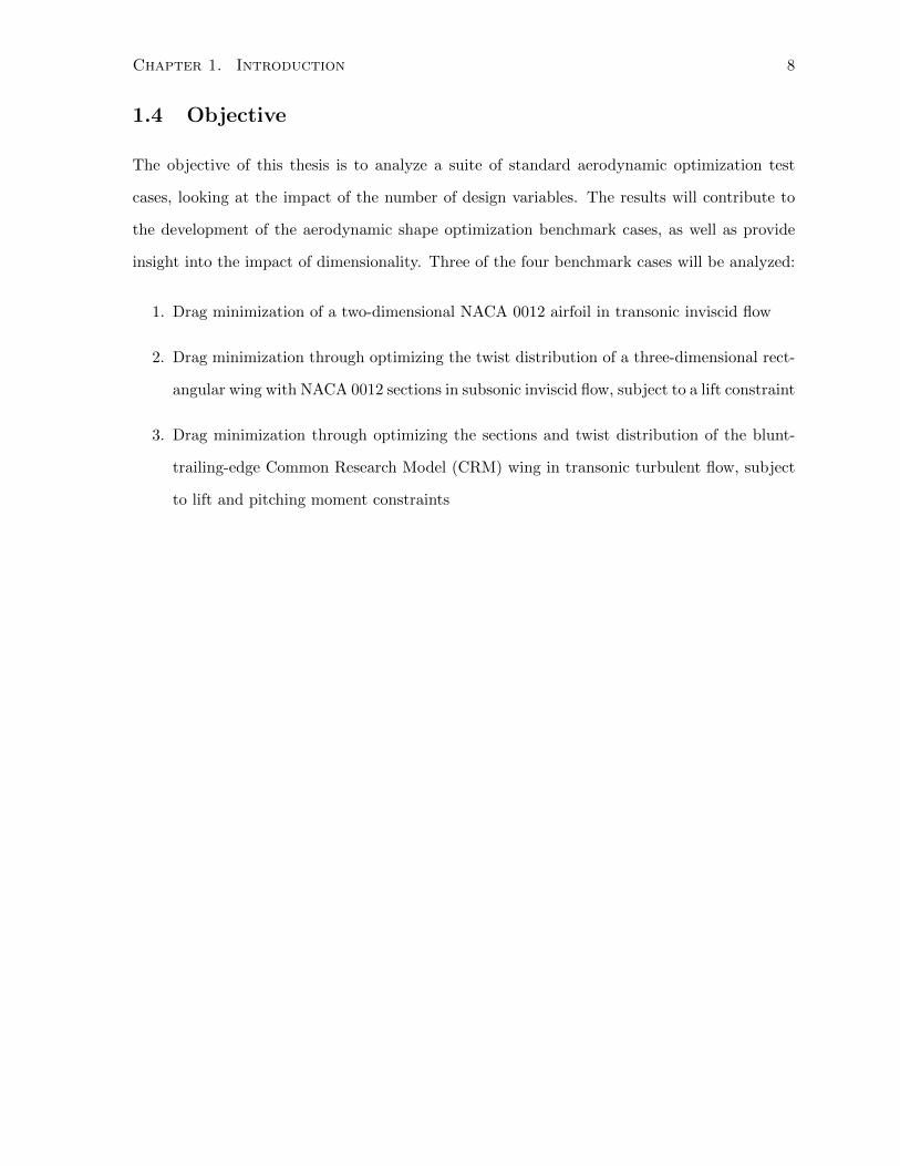
1.4 Objective
The objective of this thesis is to analyze a suite of standard aerodynamic optimization test
cases, looking at the impact of the number of design variables. The results will contribute to
the development of the aerodynamic shape optimization benchmark cases, as well as provide
insight into the impact of dimensionality. Three of the four benchmark cases will be analyzed:
1. Drag minimization of a two-dimensional NACA 0012 airfoil in transonic inviscid flow
2. Drag minimization through optimizing the twist distribution of a three-dimensional rect-
angular wing with NACA 0012 sections in subsonic inviscid flow, subject to a lift constraint
3. Drag minimization through optimizing the sections and twist distribution of the blunt-
trailing-edge Common Research Model (CRM) wing in transonic turbulent flow, subject
to lift and pitching moment constraints
Chapter 2
Algorithm
2.1 Geometry Parameterization and Mesh Movement
Geometric parameterization is employed to have a balance between the number of design vari-
ables and the ability to represent a wide variety of shapes. Numerical optimization algorithms
can only handle a finite set of variables, which requires that a geometry parameterization be
used to reduce the aerodynamic shape to a finite number of design variables. Several differ-
ent geometry parameterization techniques have been used for aerodynamic shape optimization,
each having its advantages and disadvantages. A good parameterization should be able to
approximate a wide variety of aerodynamic shapes while using as few design variables as possi-
ble. The parameterization in Jetstream uses B-spline tensor volumes to approximate not only
the surface, but the entire multi-block structured computational mesh, and was developed by
Hicken and Zingg [11]. As a result, the geometry parameterization is integrated with the mesh
movement scheme. This section will introduce how B-spline curves and volumes are utilized to
fit the surfaces and mesh blocks.
2.1.1 B-Spline Curves
A B-spline curve of order p is composed of a linear combination of control points and basis
functions:
X(ξ) =
N∑i=1
BiN (p)i (ξ) (2.1)
9
Chapter 2. Algorithm 10
where Bi are the coordinates of the de Boor control points, and N (p)i (ξ) are the B-spline basis
functions of order p (degree p−1). There are N control points used for a given parameterization.
The number of control points used will affect the accuracy with which the B-spline curve can fit
a given curve, with the minimum number of control points equal to p. A more complex shape
will require a higher number of control points to achieve a certain B-spline fitting accuracy.
The basis functions are defined according to the Cox-de-Boor recursion formula [7]:
N (1)i (ξ) =
1 if ti ≤ ξ ≤ ti+1
0 otherwise
(2.2)
N (p)i (ξ) =
ξ − titi+p−1 − ti
N (p−1)i (ξ) +
ti+p − ξti+p − ti+1
N (p−1)i+1 (ξ) (2.3)
and the basis functions are defined along a knot vector
T = (t1, t2, ..., tp−1, tp, tp+1, ..., tN−1, tN , tN+1, ..., tN+p) (2.4)
where the knot vector has N + p elements, equal to the number of control points (N) plus the
order of the basis functions (p). The multiplicity of the knots affects the continuity of the curve,
such that a knot with multiplicity m has a continuity of Cp−m−1. If the multiplicity is equal
to the order of the B-spline curve (m = p), the curve has C−1 continuity, or a discontinuity, at
that point. Enforcing this type of multiplicity at the endpoints of the knot vector ensures the
control points coincide with the data points at the beginning and end of the curve.
The order of the basis functions and the definition of the knot vector both affect the B-spline
curve. In this work, all B-spline basis functions are fourth order (p = 4). This means that the
minimum number of control points that can be used is N = 4, and a multiplicity of m = 4 is
enforced at the end points of the knot vector. The knot vector can be defined in different ways.
A uniform knot vector would have evenly spaced knot values, such that ti − ti−1 is constant
for all values of i. With this type of knot vector, enforcing multiplicity of knots is not possible.
Since we wish to have the endpoints of the curve pass through certain control points, it is
necessary to have a nonuniform knot vector.

Chapter 2. Algorithm 11
2.1.2 B-Spline Curve Fitting
The B-Spline curves presented in the previous section must be expanded in order to be useful
for fitting practical aerodynamic curves and surfaces. In order to fit a surface using a B-
spline curve, the surface must be parameterized and the knot vector must be set. A discrete
parameterization is required, so in place of ξ in the equations above, wj is used. A chord length
parameterization is used
w1 = 0 , wj =
∑j−1s=1
√Ls
LTwhere j = 2, ..., S − 1 , wS = 1 (2.5)
where S is the total number of airfoil surface points, Ls is the segment length between surface
points, and LT is the total length of all surface points.
A nonuniform knot sequence is used, given by [9]:
ti =
0 if 1 ≤ i ≤ p
1−cos( i−pN−p+1
π)
2 if p+ 1 ≤ i ≤ N
1 if N + 1 ≤ i ≤ N + p
(2.6)
Once the knot vector and parameterization are set, the B-spline basis functions can be calcu-
lated. In order to determine the locations of the control points, the following must be minimized
min
S∑j=1
‖Dj −Xj‖ (2.7)
where Dj are the surface points of the data to be fit, and Xj is the fitted curve, as defined by
equation 2.1. In order to ensure the leading edge of the airfoil is smooth, the control points
closest to the leading edge should be colinear, as shown in Figure 2.1. This can be accomplished
by moving a control point after the minimization, however this will change the fitted shape that
was obtained. Another way to accomplish this is to do a constrained minimization that sets the
colinearity through the least squares solution. In the algorithm, the colinearity is set outside
the minimization, and then the fit is adjusted using parameter correction as described in the
next section.

Chapter 2. Algorithm 12Y X
Z
Colinear control points at leading edge
Figure 2.1: Example of colinear control points at airfoil leading edge
2.1.3 Parameter Correction
With the parameterization method described in the previous sections, the vectors Dj − Xj
are not perpendicular to the tangent of the fitted curve X′j . A better fit can be obtained by
changing the values of the parameters wj through an iterative parameter correction procedure,
such as that suggested by Hoschek [13]
w̄j = wj + ∆cjtN − t1L
(2.8)
∆cj = (Dj −Xj)Yj (2.9)
where L is the total length of the control polygon defined by connecting the control points, and
Yj is the normalized tangent vector, found by calculating the derivative of the B-spline curve.
In order to demonstrate the effect of the parameter correction, it is applied to the fit of one
half of the symmetrical NACA0012 airfoil and iterated until the residual drops below 10−5, the
maximum number of iterations (1000) is reached, or the residual stops changing.
Figures 2.2 to 2.4 show how the impact of the parameter correction on the quality of the fit
depends on the number of control points. In practice, the parameter correction is implemented
on curves that compose a three-dimensional extruded airfoil or wing. This is done until the
residual drops below a tolerance of 1 × 10⁻⁶ or 1000 iterations are performed. An extruded

Chapter 2. Algorithm 13
0 0.2 0.4 0.6 0.8 1−0.07
−0.06
−0.05
−0.04
−0.03
−0.02
−0.01
0No parameter correction
Data pointsFitted points
0 0.2 0.4 0.6 0.8 1−0.07
−0.06
−0.05
−0.04
−0.03
−0.02
−0.01
0Parameter correction
Data pointsFitted points
Figure 2.2: Comparison of fitting a NACA 0012 airfoil using B-spline curves with 5 controlpoints, with and without parameter correction
0 0.2 0.4 0.6 0.8 1−0.07
−0.06
−0.05
−0.04
−0.03
−0.02
−0.01
0No parameter correction
Data pointsFitted points
0 0.2 0.4 0.6 0.8 1−0.07
−0.06
−0.05
−0.04
−0.03
−0.02
−0.01
0Parameter correction
Data pointsFitted points
Figure 2.3: Comparison of fitting a NACA 0012 airfoil using B-spline curves with 9 controlpoints, with and without parameter correction
0 0.2 0.4 0.6 0.8 1−0.07
−0.06
−0.05
−0.04
−0.03
−0.02
−0.01
0No parameter correction
Data pointsFitted points
0 0.2 0.4 0.6 0.8 1−0.07
−0.06
−0.05
−0.04
−0.03
−0.02
−0.01
0Parameter correction
Data pointsFitted points
Figure 2.4: Comparison of fitting a NACA 0012 airfoil using B-spline curves with 14 controlpoints, with and without parameter correction

Chapter 2. Algorithm 14
Streamwise Control Points
Init
ial F
it R
esid
ual
5 10 15 20
10-4
10-3
10-2
Figure 2.5: Plot of fit residual between NACA0012 airfoil and B-spline curve before parametercorrection
airfoil is composed of two curves, one which defines the upper surface and one which defines
the lower surface, that are extruded into space. For a NACA 0012 airfoil, these curves are
symmetrical about the chord. When 5 streamwise control points are used to parameterize each
surface (upper and lower) of the extruded NACA 0012 airfoil, the initial residual is 2.3× 10⁻²,
and after 1000 iterations of the parameter correction it is dropped to 8.4 × 10⁻⁵. When 9
streamwise control points are used, the residual begins at 2.1 × 10⁻³ and drops to 4.5 × 10⁻⁵
after 1000 iterations. Figure 2.5 shows how the initial residual changes with the number of
streamwise control points. As the number of control points is increased, the initial fit residual
decreases.
The parameter correction is limited in how much it can efficiently decrease the residual of
the curve fit. For example, when using 5 streamwise control points, the residual will not drop
much below 1 × 10⁻⁴, even if allowed to continue for 100,000 iterations. When 14 streamwise
control points are used, after 100,000 iterations the residual will drop from 3.39 × 10⁻⁴ to
5 × 10⁻⁶. The parameter correction can only drop the residual approximately two orders of

Chapter 2. Algorithm 15
magnitude. Using 100,000 iterations does not take much time in this case, because only a single
curve is being fit, but if multiple curves or the entire grid had the parameter correction applied,
it would not be possible to allow it to iterate so long.
Two of the cases investigated in this thesis use the parameter correction for B-spline curve
fitting to improve the initial geometry, as their geometries are composed of an extruded airfoil
in the two-dimensional case and an extruded airfoil with a pinched tip in the three-dimensional
case. The parameter correction is not applied to the more complicated Common Research
Model wing, as it is more costly to apply in three-dimensions.
2.1.4 B-Spline Surfaces and Volumes
The concepts that were explained in the previous sections for B-spline curves can be extended
to produce B-spline surfaces and B-spline volumes. This allows parameterization of the aero-
dynamic surface and the entire computational grid. For a B-spline volume, the curve definition
in equation 2.1 becomes
X(ξ) =
Ni∑i=1
Nj∑j=1
Nk∑k=1
BijkNi(ξ)Nj(η)Nk(ζ) (2.10)
where X(ξ) represents the coordinates of the nodes of the computational mesh as a function
of curvilinear coordinates ξ = (ξ, η, ζ). The basis functions calculated in the ξ direction, while
holding η and ζ constant, are
N (1)i (ξ; η, ζ) =
1 if ti(η, ζ) ≤ ξ ≤ ti+1(η, ζ)
0 otherwise
(2.11)
N (p)i (ξ; η, ζ) =
ξ − ti(η, ζ)
ti+p−1(η, ζ)− ti(η, ζ)N (p−1)i (ξ; η, ζ) +
ti+p(η, ζ)− ξti+p(η, ζ)− ti+1(η, ζ)
N (p−1)i+1 (ξ; η, ζ)
(2.12)

Chapter 2. Algorithm 16
with similar expressions for the η and ζ directions. The knot vector, ti(η, ζ), is a spatially
varying function that depends on η and ζ. The basis functions are defined along a knot vector
ti(η, ζ) = (1− η)(1− ζ)ti(0, 0) + η(1− ζ)ti(1, 0) + (1− η)ζti(0, 1) + ηζti(1, 1) (2.13)
where ti(0, 0), ti(1, 0), ti(0, 1) and ti(1, 1) are the edge knot values, which are constant. As with
the B-spline curve, the surface must be parameterized, and a chord-length parameterization is
used. The system is solved using a least-squares fitting, with the block edges fit first, followed
by the surfaces, and finally the internal volume control points. The final B-spline volume
mesh maintains the relative spacing of the original computational mesh, but is several orders of
magnitude smaller. Without this property, areas with high curvature would not be accurately
resolved.
2.1.5 Mesh Movement
In order for aerodynamic shape optimization to occur, geometry changes must be accommo-
dated by both the parameterization and the mesh movement schemes. By fitting the compu-
tational mesh with B-spline volumes, changes in the control points on the B-spline surface can
be propagated through the mesh using a method based on the principles of linear elasticity,
which was adapted from the work of Truong et al. [26] by Hicken and Zingg [12]. Using a
method based on linear elasticity is typically computationally expensive; however, the control
mesh made up of the B-spline volume control points is up to two orders of magnitude smaller
than the full computational mesh, allowing the computational time to be much lower.
The volumes of the control mesh are treated as linear elastic solids that are isotropic and
homogeneous, with a Poisson’s ratio of ν = −0.2 to prevent a high aspect ratio. The Young’s
modulus is proportional to the inverse of the cell volume. To accommodate large shape changes
and improve robustness, the mesh movement occurs in increments. This work uses m = 5
increments, but if mesh movement problems occur, it is possible to use more increments. The
intermediate control points are related to their initial b(0)s and final b
(m)s values using a linear

Chapter 2. Algorithm 17
relationship
b(i)s = i
m(b(m)s − b(0)s ) + b
(0)s , i = 1, ...,m. (2.14)
Equation 2.14 is discretized on the control mesh using a finite-element method. The resulting
linear system is solved using the conjugate gradient method preconditioned with ILU(1) [18],
with the convergence criterion being a reduction in the L2 norm to a relative tolerance of 10−12.
The fine mesh is then updated based on the control mesh using an algebraic approach that is
based on the B-spline volume basis functions.
2.2 Flow Solver
The flow solver is one of the key components of any aerodynamic shape optimization algorithm.
The flow solver should be efficient, accurate and robust. Accuracy is required to allow the
optimizer to use the information from the flow solver to produce an optimum solution. Efficiency
is required as the optimizer will perform many flow solves through the course of an optimization.
Robustness is necessary to accommodate significant geometry changes. This section presents
an overview of the parallel three-dimensional multi-block structured solver used in Jetstream.
The flow solver uses the Newton-Krylov method to obtain high-fidelity flow solutions for use
within the aerodynamic shape optimization algorithm. The flow solver was developed by Hicken
and Zingg [10] for the three-dimensional Euler equations, and by Osusky and Zingg [22] for the
three-dimensional RANS equations. The flow solver algorithm solves the three-dimensional
RANS equations for viscous turbulent flows, and the Euler equations for inviscid flows. The
RANS equations are fully coupled with the Spalart-Allmaras one-equation turbulence model.
The governing equations are discretized using second-order Summation-by-Parts (SBP) opera-
tors. Boundary conditions and block interfaces use Simultaneous Approximation Terms (SATs).
An implicit Euler time marching scheme is applied with an increasing time step, eventually be-
coming an inexact-Newton method, producing a large, sparse system of linear equations that
is solved using flexible GMRES (FGMRES) . An approximate Newton start-up phase is used
to provide the initial iterate for the inexact-Newton phase.

Chapter 2. Algorithm 18
2.3 Optimization Algorithm
The optimization algorithm used is called SNOPT (Sparse Nonlinear OPTimizer) and was
developed by Gill, Murray and Saunders [8]. It is a gradient based optimizer, capable of finding
a local optimum for a constrained optimization problem of the form
minimize f(x), x ∈ Rn
subject to ci(x) = 0, i ∈ E
ci(x) ≥ 0, i ∈ I
where the vector, x, contains the design variables, typically coordinates of the geometric control
points and angle of attack. The objective function, f(x), is often the drag coefficient or the
ratio of drag to lift. The vector, c(x), contains the constraint functions, which can be linear or
nonlinear and are expressed using an equality (i ∈ E) or inequality (i ∈ I).
On large problems, SNOPT performs most efficiently if only some of the variables enter
the problem nonlinearly or if there are relatively few degrees of freedom at a solution (meaning
many of the inequality constraints are at their bounds). For an aerodynamic shape optimization
problem, where the lift and drag coefficients depend on the geometry, all the design variables
will enter the problem nonlinearly, as lift and drag are nonlinear functions of the design vari-
ables. It is therefore reasonable to expect that as the number of design variables increases, the
convergence of the optimizer will be affected, as demonstrated by Zingg et al. [29]. In addition,
the presence of more design variables can impact the convergence of the mesh movement al-
gorithm or produce geometries that cannot achieve a converged flow solution. When either of
these situations occur, SNOPT must find a way back into a region where these functions are
defined by shortening the step length it takes along the search direction. If it is not able to get
back into a region with defined functions (meaning that both the mesh movement algorithm
and the flow solver converge) using this method, the algorithm will terminate.

Chapter 2. Algorithm 19
2.3.1 Gradient Evaluation
To use a gradient-based optimization method, the gradient must be computed accurately and
efficiently. Using finite differencing is not possible for the problems in question, as there are too
many design variables, and it would be prohibitively inefficient. Pironneau [24] and Jameson [15]
proposed the adjoint method, which allows the gradient to be computed at a cost that is virtually
independent of the number of design variables. The present work uses the discrete adjoint
method, rather than the continuous form. The mesh movement and flow residual equations are
treated as nonlinear constraints that are solved outside of SNOPT. These nonlinear constraints
are linearized analytically to form the adjoint gradient.
The flow Jacobian matrix is formed by linearizing the components of the discrete flow
residual, including the viscous and inviscid fluxes, the numerical dissipation, the turbulence
model, and the boundary conditions. This linearization was completed by Hicken and Zingg
[11] and Osusky [19]. The pressure switch was not linearized in the algorithm developed by
Hicken and Zingg, but was instead treated as a constant in the evaluation of the flow Jacobian.
Osusky introduced the full linearization. The pressure switch is used for capturing shocks,
and is important to use for transonic flows. It was shown that omitting the pressure switch
from the gradient only introduces small errors, which is not problematic for problems that are
shock-free at the final geometry. However, one of the cases investigated in this thesis is inviscid
and transonic, and the geometries produced are not shock-free. For this case, it was found that
if the pressure switch is turned on, but its linearization is not included, the total gradient is
inaccurate and the optimization algorithm cannot converge. If the pressure switch is turned
off, the drag and lift coefficients obtained are inaccurate. Figure 2.6 shows the effect of the
pressure switch on the drag minimization of a two-dimensional NACA 0012 airfoil in inviscid,
transonic flow at zero angle of attack with a lift constraint of zero. This is performed on the
algorithm Optima2D, which does not include the linearization of the pressure switch. In order
to achieve a converged optimization, the pressure switch was turned off to prevent having an
inaccurate gradient. When the final optimized geometries were analyzed by performing a flow
solve with the pressure switch turned on, the drag coefficients obtained were shown to be much
higher than those obtained without the pressure switch, and the lift constraint was no longer

Chapter 2. Algorithm 20
Number of Control Points
Fin
al D
rag
Co
effi
cien
t
0 10 20 30
0.005
0.01
0.015
0.02
0.025
0.03
0.035
0.04
0.045
Optima2D results with pressure switch offOptima2D with pressure switch on
Figure 2.6: Effect of pressure switch on optimization of inviscid, transonic NACA 0012 airfoilat zero angle of attack
met.
Figure 2.7 shows a Mach contour for the final optimized shape of the airfoil using 20 design
variables. Without the pressure switch on, this contour looks symmetrical, and the lift con-
straint is met. When this same geometry is analyzed with the pressure switch on, it is clear the
flow is no longer symmetrical across the airfoil chord, and the lift constraint is not met. There
is a shock on the upper surface of the airfoil. Although the airfoil is symmetric, it is producing
a lifting, or non-unique, solution. Ou et al. [23] analyzed four different symmetrical airfoils,
showing that they exhibited non-unique solutions in a range of transonic Mach numbers. The
Mach number, M = 0.85, used for this pressure switch analysis falls within this range. Further
analysis of the non-unique solutions produced by this case is recommended.
In summary, the pressure switch is necessary to accurately capture the flow conditions at
transonic Mach numbers. If the pressure switch is not linearized and included in the flow Jaco-
bian, the resulting gradient may be so inaccurate that it prevents the optimization algorithm
from achieving a converged solution. This inaccuracy is most pronounced for cases where the
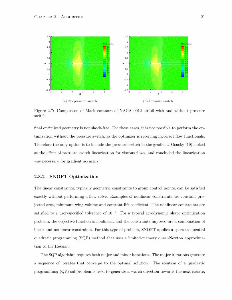
Chapter 2. Algorithm 21
X
Y
-2 -1 0 1 2 3-2.5
-2
-1.5
-1
-0.5
0
0.5
1
1.5
2
2.5
Mach Number
1.51.41.31.21.110.90.80.70.60.50.40.30.20.1
(a) No pressure switch
X
Y
-2 -1 0 1 2 3-2.5
-2
-1.5
-1
-0.5
0
0.5
1
1.5
2
2.5
Mach Number
1.51.41.31.21.110.90.80.70.60.50.40.30.20.1
(b) Pressure switch
Figure 2.7: Comparison of Mach contours of NACA 0012 airfoil with and without pressureswitch
final optimized geometry is not shock-free. For these cases, it is not possible to perform the op-
timization without the pressure switch, as the optimizer is receiving incorrect flow functionals.
Therefore the only option is to include the pressure switch in the gradient. Osusky [19] looked
at the effect of pressure switch linearization for viscous flows, and concluded the linearization
was necessary for gradient accuracy.
2.3.2 SNOPT Optimization
The linear constraints, typically geometric constraints to group control points, can be satisfied
exactly without performing a flow solve. Examples of nonlinear constraints are constant pro-
jected area, minimum wing volume and constant lift coefficient. The nonlinear constraints are
satisfied to a user-specified tolerance of 10−6. For a typical aerodynamic shape optimization
problem, the objective function is nonlinear, and the constraints imposed are a combination of
linear and nonlinear constraints. For this type of problem, SNOPT applies a sparse sequential
quadratic programming (SQP) method that uses a limited-memory quasi-Newton approxima-
tion to the Hessian.
The SQP algorithm requires both major and minor iterations. The major iterations generate
a sequence of iterates that converge to the optimal solution. The solution of a quadratic
programming (QP) subproblem is used to generate a search direction towards the next iterate,

Chapter 2. Algorithm 22
which is solved via minor iterations. It is in the solution of the QP subproblem where the
impact of the number of degrees of freedom is seen. The QP subproblem employs a two-phase
active-set algorithm that solves
minimize fk + gTk (x− xk) +1
2(x− xk)THk(x− xk) (2.15)
subject to ck + Jk(x− xk) ≥ 0 (2.16)
where fk is the objective function, gk is the gradient of the objective function, and the vector
x contains the design variables. The matrix, Hk, is a quasi-Newton approximation to the Hes-
sian of the Lagrangian, and is updated after each major iteration using BFGS. The nonlinear
constraints and linear constraints are converted to equalities using slack variables. The non-
linear constraints are then linearized. The second equation represents this linearization of the
nonlinear constraints, where the vector ck contains the nonlinear constraints, and the gradients
of these constraints form the Jacobian, Jk. At each minor iteration the constraints, ck, are
partitioned into basic, superbasic and nonbasic variables:
BxB + SxS +NxN = b (2.17)
The nonbasic variables are frozen at their upper and lower bounds, and therefore made
active and part of the working active set for the minor iteration. An inequality constraint is
considered active at a solution if
ci(x) = 0, i ∈ I (2.18)
meaning the constraint is at its bound. A search direction is sought that moves the superbasic
variables in a direction that will improve the objective function. The basic variables change
to satisfy the constraint equation and the nonbasic variables remain the same. The search
direction then satisfies:
BpB + SpS = 0 (2.19)
The superbasic variables represent the number of degrees of freedom that remain after the

Chapter 2. Algorithm 23
constraints are satisfied. The search direction is computed using the reduced-Hessian and the
reduced-gradient. The method used to calculate this depends on the number of superbasic
variables. When no more improvement can be found in the objective function, a nonbasic
variable is added to the superbasic variable set, decreasing the working active set. In contrast,
the working active set is increased by one when the step size is too large such that it violates
the bounds of a basic or superbasic variable.
An optimization is deemed successful, or fully converged, when SNOPT is able to satisfy
the KKT conditions to within a specified tolerance. The nonlinear constraints must be satisfied
to within a tolerance of 10−6, referred to as the feasibility tolerance. The gradient of the
Lagrangian must also meet a tolerance, referred to as the optimality tolerance, which is user
specified and can vary from problem to problem, but ranges from 10−5 to 10−7.

Chapter 3
Results
3.1 Case 1: Symmetrical Airfoil Optimization in Transonic In-
viscid Flow
This case involves drag minimization of the NACA 0012 airfoil in transonic, inviscid flow and is
based on work done by Vassberg et al. [27] The number of control points used to parameterize
the airfoil is varied to investigate the effect the parameterization has on the optimization. In
a two-dimensional inviscid flow, the only source of drag, other than numerical error (including
the effect of the finite distance to the far-field boundary), is wave drag. Hence if the shocks can
be eliminated, the drag is strictly a consequence of numerical error.
3.1.1 Optimization Problem
The optimization problem can be summarized as
minimize CD
wrt z
subject to z ≥ zbaseline
where CD is the drag coefficient, z is the vertical coordinate of the optimized geometry, and
zbaseline is the vertical coordinate of the baseline geometry. The geometry is subject to a min-
25
Chapter 3. Results 26
imum thickness constraint which requires the optimized geometry to be greater in thickness
than the baseline geometry. The thickness constraint is enforced by using 7 nonlinear thickness
constraints at 15%, 20%, 22%, 24%, 26%, 29%, and 35% chord, as done by Bisson, Nadarajah
and Dong [3]. These locations are chosen because the optimizer search direction tries to reduce
the airfoil thickness in this region. The thickness at other chordwise locations will be confirmed
after the final shape is obtained to ensure the thickness constraint is not violated. The use of
nonlinear constraints is preferred in place of linear constraints on the control points, as it is
independent of the initial fit of the airfoil. Since the B-spline fit is not exact, the initial fit of
the NACA 0012 airfoil can vary slightly based on the number of control points used. If the
constraints are placed on the control points, rather than the surface itself, the optimization
problem is changed slightly when the parameterization is changed. Using nonlinear thickness
constraints that constrain the surface ensures that the optimization problem is identical regard-
less of the parameterization. Since the initial airfoil is symmetric, the resulting lift coefficient is
zero, which should be maintained throughout the optimization. The symmetry is enforced by
adding linear constraints to the control points on the upper and lower surfaces that force them
to be equal and opposite in sign. The optimization is given an optimality tolerance of 10−7;
however, not all cases are able to achieve this level of convergence. The feasibility tolerance for
nonlinear constraints is 10−6.
3.1.2 Flow Conditions
The flow is inviscid and transonic with a freestream Mach number of M = 0.85 and zero angle
of attack (α = 0◦).
3.1.3 Initial Geometry
The NACA 0012 airfoil is modified to have a zero thickness trailing edge. The modified airfoil
is defined as
zbaseline = ±0.6(0.2969√x− 0.1260x− 0.3516x2 + 0.2843x3 − 0.1036x4), x ∈ [0, 1], (3.1)

Chapter 3. Results 27
Y X
Z
X Y
Z
X
Y
Z
Y X
Z
Figure 3.1: NACA 0012 extruded airfoil initial geometry
where the modification to the trailing edge occurs via a change in the x4 term. In order
to use the three-dimensional optimization algorithm, the optimization is performed using an
extruded airfoil. The airfoil is extruded one chord length, so it has a chord of one unit and a
span of one unit. The extruded airfoil is composed of an upper and lower patch. Each patch
is parameterized using a variable number of control points in the streamwise direction and a
constant number of control points (five) in the spanwise direction. Figure 3.1 shows the initial
geometry parameterized with fourteen streamwise control points on each surface.
3.1.4 Grid
A structured grid is created around a flat plate with a chord length of one unit and a span of
one unit. The mesh movement capabilities of the algorithm are then used to inflate this flat
plate into an extruded airfoil with the sections determined from the B-spline fit of the NACA
0012 airfoil. Just as the geometry can be thought of as the extrusion of a two-dimensional
airfoil, the grid can be thought of as an extrusion of a two-dimensional grid. There are ten
nodes in the extruded direction, meaning the three-dimensional grid is ten times larger than its
equivalent two-dimensional grid. Three different grid levels are created by starting with a fine
grid and removing every other grid node, except in the extruded direction where the number
of nodes remains constant. The fourth grid level (superfine) is created by refining the fine grid
by doubling the number of nodes in the streamwise and offwall direction. Figure 3.2 shows the
coarse grid level.

Chapter 3. Results 28
Y X
Figure 3.2: Coarse grid level for NACA 0012 extruded airfoil
Grid Study - Initial Geometry
Table 3.1 outlines the number of nodes, the streamwise spacing at the leading and trailing
edges, and the off-wall spacing of the different grid levels. The number of nodes reported is
the two-dimensional equivalent, calculated by taking the total number of nodes in the three-
dimensional grid and dividing by ten (the number of nodes in the extruded direction). A grid
study of the initial geometry is conducted by performing a flow solve on each grid level. The fine
grid is inflated using a parameterization with 48 streamwise control points on the upper and
lower surfaces. A relatively high number of control points is chosen to ensure a highly accurate
B-spline fit of the airfoil. The next two grid levels are created by subsequently removing every
other node in the streamwise and offwall direction. The superfine grid level is created by refining
the fine grid then splitting the blocks. Table 3.2 shows that the medium and fine grid levels are
within 3/10 of a drag count of each other. The fine and superfine grid levels produce the same
drag coefficient of 457.327 drag counts. Vassberg et al. [27] obtained an initial drag coefficient
of 468.9 drag counts, while Bisson et al. [3] obtained an initial drag of 464.2 drag counts on
their finest grid. Carrier et al. [5] obtained a zero mesh size drag coefficient of 471.1 counts.
The initial drag coefficient obtained by Jetstream on the superfine grid is 7 counts below the
lowest value obtained by Bisson et al.

Chapter 3. Results 29
Table 3.1: Grid parameters for NACA 0012 airfoil grid study
Grid Nodes (2D)Off-wallSpacing
Leading-EdgeSpacing
Trailing-EdgeSpacing
Coarse 12760 0.008 0.008 0.008Medium 49020 0.004 0.004 0.004
Fine 192100 0.002 0.002 0.002Superfine 768400 0.001 0.001 0.001
Table 3.2: Results of grid study for NACA 0012 airfoil inflated using 48 streamwise controlpoints per patch
Grid Level Nodes (2D)Drag Coefficient
(Counts)
Coarse 12760 461.299Medium 49020 457.598
Fine 192100 457.327Superfine 768400 457.327
3.1.5 Optimization Results
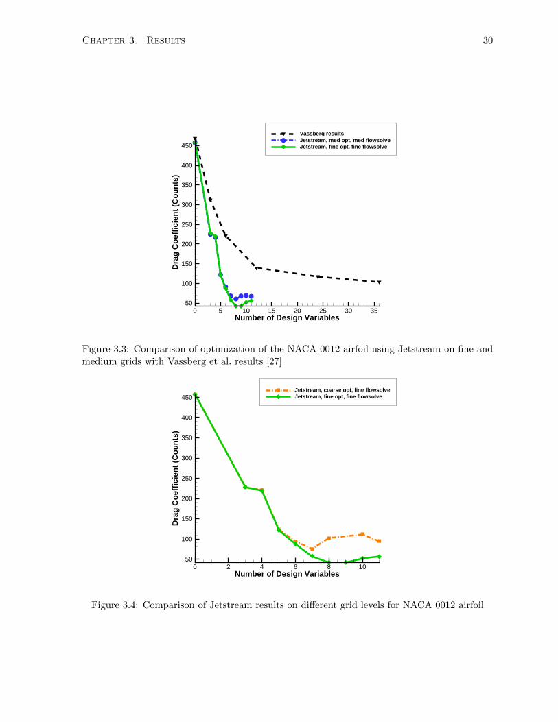
The results of the optimization using Jetstream can be compared to those obtained by Vassberg
et al. [27] They used a Bezier curve geometry parameterization along with a response-surface
optimization approach. Optimization using Jetstream is performed on the coarse, medium and
fine grid levels. Figure 3.3 shows the results obtained performing optimization using Jetstream
and compares them to those obtained by Vassberg et al. The number of control points used
to parameterize each surface in the streamwise direction is varied from 5 to 13. The leading
and trailing edge control points are fixed, and the movement of the lower surface control points
is constrained to be symmetric to the upper surface control points. The number of design
variables for each case is then equal to the number of streamwise control points per surface,
subtracting the two fixed control points. Therefore, the number of design variables is varied
from 3 to 11. The drag coefficients obtained by Jetstream are significantly lower than those
obtained by Vassberg et al., where the lowest drag coefficient obtained is 103.8 drag counts. One
explanation for this could be grid density. The grid used by Vassberg et al. has 65,536 nodes,
compared to the 2D-equivalent of 192,100 for the fine grid used with Jetstream. However, the
medium grid, which has a similar grid density at 49,020 nodes, is also able to achieve lower
drag values. Another explanation for the lower drag values is the parameterization used. The
Bezier curve parameterization used by Vassberg et al. has very few design variables near the
Chapter 3. Results 30
Number of Design Variables
Dra
g C
oef
fici
ent
(Co
un
ts)
0 5 10 15 20 25 30 3550
100
150
200
250
300
350
400
450
Vassberg resultsJetstream, med opt, med flowsolveJetstream, fine opt, fine flowsolve
Figure 3.3: Comparison of optimization of the NACA 0012 airfoil using Jetstream on fine andmedium grids with Vassberg et al. results [27]
Number of Design Variables
Dra
g C
oef
fici
ent
(Co
un
ts)
0 2 4 6 8 1050
100
150
200
250
300
350
400
450Jetstream, coarse opt, fine flowsolveJetstream, fine opt, fine flowsolve
Figure 3.4: Comparison of Jetstream results on different grid levels for NACA 0012 airfoil

Chapter 3. Results 31
Design Iteration
Op
tim
alit
y
5 10 15 20 25 30 35 40 45 5010-7
10-6
10-5
10-4
10-3
10-2
Figure 3.5: Typical convergence histories for NACA 0012 airfoil optimization
trailing edge, whereas the B-spline curve parameterization has more design variables in this
region. The B-spline parameterization has roughly half of the design variables in the first 50%
of chord length measured from the leading edge, and half in the second 50%. With the Bezier
parameterization, 5/6 of the design variables are within the first 50% of chord length, and 1/6
of the design variables are in the second 50%. Since the majority of the geometry change is
occurring near the trailing edge, the B-spline parameterization is better suited than the Bezier
parameterization, as shown by Carrier et al. [5] Looking at the optimization results on the fine
grid, as the number of design variables increases, the drag obtained decreases. The lowest drag
coefficient is obtained on the fine grid level with 9 design variables: 42.24 drag counts, which
is a reduction of 91% relative to the baseline geometry. However, after 9 design variables, the
drag increases slightly. Figure 3.4 compares the results of optimization using the coarse grid
(with a flowsolve on the final geometry using the fine grid) to optimization using the fine grid.
In all cases the final drag obtained on the fine grid is lower than that obtained on the coarse
grid. Using 3, 4, and 5 design variables, this difference is 2 drag counts or less. With 6 design
variables the fine grid optimization produces a geometry almost 6 drag counts lower than that
from the coarse grid, and with 8 design variables the difference is approximately 60 drag counts.
As the number of design variables increases, the convergence of the optimizer is adversely
Chapter 3. Results 32
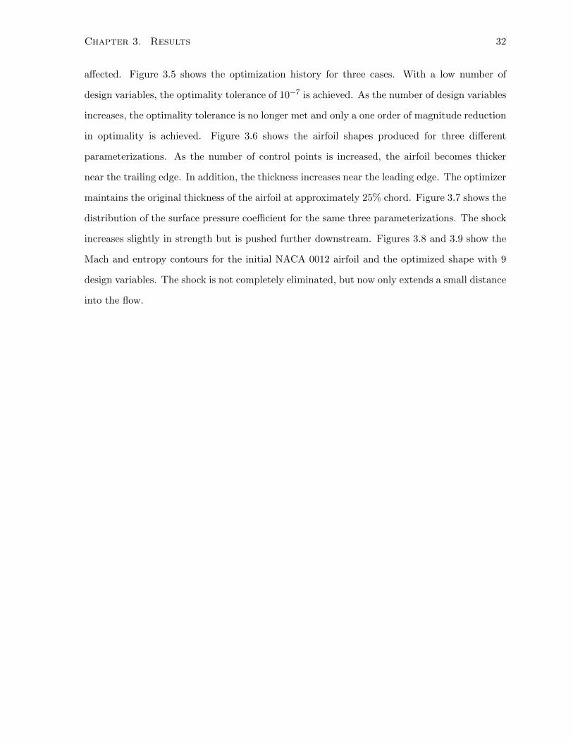
affected. Figure 3.5 shows the optimization history for three cases. With a low number of
design variables, the optimality tolerance of 10−7 is achieved. As the number of design variables
increases, the optimality tolerance is no longer met and only a one order of magnitude reduction
in optimality is achieved. Figure 3.6 shows the airfoil shapes produced for three different
parameterizations. As the number of control points is increased, the airfoil becomes thicker
near the trailing edge. In addition, the thickness increases near the leading edge. The optimizer
maintains the original thickness of the airfoil at approximately 25% chord. Figure 3.7 shows the
distribution of the surface pressure coefficient for the same three parameterizations. The shock
increases slightly in strength but is pushed further downstream. Figures 3.8 and 3.9 show the
Mach and entropy contours for the initial NACA 0012 airfoil and the optimized shape with 9
design variables. The shock is not completely eliminated, but now only extends a small distance
into the flow.

Chapter 3. Results 33
X
Z
0 0.2 0.4 0.6 0.8 10
0.01
0.02
0.03
0.04
0.05
0.06
0.073 DVs Surface Points6 DVs Surface Points9 DVs Surface PointsNACA Surface Po
Figure 3.6: Comparison of final optimized airfoil shapes to initial NACA 0012 airfoil
X
Pre
ssu
re C
oef
fici
ent
0 0.2 0.4 0.6 0.8 1
-1.5
-1
-0.5
0
0.5
1
1.5
NACA 00123 DVs6 DVs9 DVs
Figure 3.7: Comparison of final coefficient of pressure distributions to initial NACA 0012 airfoil

Chapter 3. Results 34
(a) Initial NACA 0012 Airfoil (b) Final, 9 Design Variables
Figure 3.8: Comparison of Mach contours for initial NACA 0012 airfoil and final optimizedshape with 9 design variables
(a) Initial NACA 0012 Airfoil (b) Final, 9 Design Variables
Figure 3.9: Comparison of entropy contours for initial NACA 0012 airfoil and final optimizedshape with 9 design variables

Chapter 3. Results 35
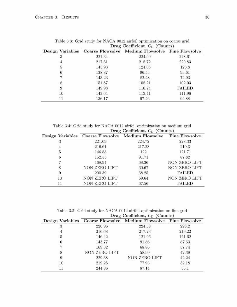
Grid Study - Final Geometry
Tables 3.3 to 3.5 show the results of a grid study on the final geometries for a variety of
parameterizations. Each table is based on the final optimized geometries using the coarse,
medium and fine grids, respectively. The final geometries are analyzed by performing a flow
solve on each grid level. For example, in Table 3.3, the optimization is performed on the coarse
grid, and then the final shape is analyzed using the medium and the fine grid. Unlike the grid
study for the initial geometry, where there is a difference of less than 1 drag count between the
medium and fine grids, the final geometries show a larger difference between the medium and
fine grid levels. For the optimizations run using the medium grid, at higher parameterizations
the flow solve either fails to converge on the coarse or fine grid level, or produces a solution with
a non-zero lift coefficient. The failed flow solves only occur on the fine grid level, suggesting
that the fine grid is resolving difficult flow features that were not present on the coarser grid
levels. Given the presence of non-unique solutions for this case, it is likely that the flow is
unsteady, but further analysis is required. For the fine optimization, fine flow solve case with
10 design variables, the order of accuracy is calculated to be p = 2.46, and the grid converged
value of drag is C∗D = 46.4 drag counts. Comparing to the grid converged value of drag for the
initial geometry, C∗D = 457.3 drag counts, this is a reduction of 90%. A grid converged value of
drag for the best case, with 9 design variables, could not be calculated due to the non-unique
solution obtained on the medium grid.
Chapter 3. Results 36
Table 3.3: Grid study for NACA 0012 airfoil optimization on coarse gridDrag Coefficient, CD (Counts)
Design Variables Coarse Flowsolve Medium Flowsolve Fine Flowsolve
3 221.34 224.99 228.614 217.31 218.72 220.835 145.93 124.05 123.86 138.87 96.53 93.617 143.23 82.48 74.938 151.87 108.21 102.039 149.98 116.74 FAILED10 143.64 113.41 111.9611 136.17 97.46 94.88
Table 3.4: Grid study for NACA 0012 airfoil optimization on medium gridDrag Coefficient, CD (Counts)
Design Variables Coarse Flowsolve Medium Flowsolve Fine Flowsolve
3 221.09 224.72 228.334 216.61 217.28 219.35 146.88 122 121.716 152.55 91.71 87.827 168.94 68.36 NON ZERO LIFT8 NON ZERO LIFT 60.67 NON ZERO LIFT9 200.39 68.25 FAILED10 NON ZERO LIFT 69.64 NON ZERO LIFT11 NON ZERO LIFT 67.56 FAILED
Table 3.5: Grid study for NACA 0012 airfoil optimization on fine gridDrag Coefficient, CD (Counts)
Design Variables Coarse Flowsolve Medium Flowsolve Fine Flowsolve
3 220.96 224.58 228.24 216.68 217.23 219.225 146.42 121.96 121.626 143.77 91.86 87.637 169.32 68.86 57.748 NON ZERO LIFT 58.99 42.399 229.38 NON ZERO LIFT 42.2410 219.25 77.93 52.1811 244.86 87.14 56.1

Chapter 3. Results 37
3.2 Case 2: Twist Optimization of a Rectangular Wing in Sub-
sonic Inviscid Flow
The second case investigated is the drag minimization of a rectangular wing with NACA 0012
sections through optimization of the twist distribution about the trailing edge. The number
of design variables is varied to investigate the effect on the optimization. The flow is subsonic
and inviscid; hence the goal is to minimize the induced drag at a fixed lift coefficient. The
optimization should recover a lift distribution that is close to elliptical and a span efficiency
factor close to one. The span efficiency factor is calculated using
e =C2L
πΛCDi
(3.2)
where e is the span efficiency factor, CL is the lift coefficient, Λ is the aspect ratio and CDi is
the induced drag coefficient.
3.2.1 Optimization Problem
The optimization problem is formally described as
minimize CD
wrt twist
subject to CL = 0.375
where CD is the drag coefficient and CL is the lift coefficient. The wing is twisted about the
trailing edge at a finite number of spanwise stations through the use of linear constraints. This is
accomplished by varying the z coordinates, so the projected surface area remains constant. The
span and aspect ratio are also fixed, so the only mechanism to reduce the induced drag coefficient
is through the span efficiency factor, which is related to the spanwise load distribution. The tip
is constrained to be a linear shear of the twist of the last two spanwise stations. This prevents
the optimizer from twisting the tip so drastically that it creates a winglet. The lift constraint
is the only nonlinear constraint implemented. The angle of attack is a design variable, and the

Chapter 3. Results 38
Figure 3.10: NACA 0012 rectangular wing initial geometry
root section is fixed. The optimization is given an optimality tolerance of 10−6; however, as in
the first case, not all cases are able to achieve this level of convergence. The feasibility tolerance
is 10−6.
3.2.2 Flow Conditions
The flow is invisicid and subsonic. The freestream Mach number is M = 0.5, and the initial
angle of attack is α = 4.4◦.
3.2.3 Initial Geometry
The geometry is a rectangular wing with NACA 0012 sections which have been modified to have
a sharp trailing edge (see Equation 3.1). The wing has a semispan of 3.06 chords, consisting of
3 chords of rectangular planform and 0.06 chords of wing-tip cap. The geometry has sixteen
surface patches, twelve inboard (upper and lower) that have a variable spanwise parameteriza-
tion and four outboard (upper and lower) that have a constant spanwise parameterization to
ensure a consistent tip geometry. Figure 3.10 shows the geometry with 13 streamwise and 11
spanwise control points on each inboard patch.
3.2.4 Grid
The grid has approximately 1.4 million nodes. The off-wall spacing is 0.002 chords, the stream-
wise leading-edge spacing is 0.005 chords, and the streamwise trailing-edge spacing is 0.01

Chapter 3. Results 39
Y
Figure 3.11: Grid for NACA 0012 rectangular wing at root
Table 3.6: Coefficients for rectangular wing with NACA 0012 sections on optimization meshand fine mesh
Initial Geometry Optimized GeometryMesh Size (nodes) 1.4× 10⁶ 11.2× 10⁶ 1.4× 10⁶ 11.2× 10⁶
CL 0.375 0.375 0.375 0.375
CD 0.00784 0.00773 0.00761 0.00759
chords. Figure 3.11 shows a close-up of the node distribution around the grid at the root.
Grid Study
A finer grid is created by doubling the number of nodes in each direction, and then splitting
the blocks to ensure a reasonable number of nodes per processor. This grid has approximately
10.2 million nodes, with an off-wall spacing of 0.001 chords, a streamwise leading-edge spacing
of 0.0025 chords and a streamwise trailing-edge spacing of 0.005 chords. Table 3.6 shows the
results of analyzing the initial and final geometry on the finer grid. The final geometry is from
the best case studied, which used 13 streamwise and 11 spanwise control points on each inboard
patch. On the coarse grid, the drag coefficient is reduced 2.3 drag counts from initial to final,
which is 3% of the initial drag. On the fine grid, the drag coefficient is reduced 1.4 drag counts
from initial to final, which is 1.8% of the initial drag. This shows that the improvement in drag
coefficient carries over to finer grid levels.

Chapter 3. Results 40
Spanwise CPs
Fin
al D
rag
Co
effi
cien
t (C
ou
nts
)
5 6 7 8 9 10 11
76.12
76.14
Figure 3.12: Effect of change in number of spanwise control points per inboard patch on finaldrag coefficient for NACA 0012 rectangular wing twist optimization case
3.2.5 Optimization Results
Figure 3.12 shows how the final drag coefficient changes as the number of spanwise control
points per inboard patch increases. The number of spanwise control points is varied from 5 to
11, and as the number increases, the final drag obtained decreases. The drag coefficient for the
untwisted wing is 78.4 drag counts, and the drag coefficient for the final optimized geometry
with 11 spanwise control points is 76.1 drag counts, which is a reduction of 3%. The difference
between the coarsest parameterization with 5 control points and the finest parameterization
with 11 control points is 0.09 drag counts. Figures 3.13 and 3.14 show how the span efficiency
factor changes as the number of spanwise control points increases. The initial spanwise efficiency
factor for the untwisted wing is 0.951, and the final span efficiency factor varies from 0.979 with 5
spanwise control points to 0.980 with 11 spanwise control points. The increase in span efficiency
is 3% from initial to final.
Figure 3.15 shows the optimization convergence history for two different parameterizations.
Both have very similar convergence histories, and the optimality is decreased four orders of
magnitude to reach the optimality tolerance of 10−6. All cases were able to achieve this required
tolerance. Figure 3.16 shows the lift distribution for the case with 11 spanwise control points.

Chapter 3. Results 41
Spanwise CPs
Eff
icie
ncy
5 6 7 8 9 10 110.95
0.955
0.96
0.965
0.97
0.975
0.98
Initial EfficiencyFinal Efficiency
Figure 3.13: Effect of change in number of spanwise control points per inboard patch on finalspan efficiency factor for NACA 0012 rectangular wing twist optimization case
Spanwise CPs
Ch
ang
e in
Eff
icie
ncy
5 6 7 8 9 10 11
0.0278
0.028
0.028
Figure 3.14: Effect of change in number of spanwise control points per inboard patch on changein span efficiency factor for NACA 0012 rectangular wing twist optimization case

Chapter 3. Results 42
Design Iteration
Op
tim
alit
y
5 10 15 20 25 30 35 40 45
10-6
10-5
10-4
10-3
10-2
5 Spanwise Control Points11 Spanwise Control Points
Figure 3.15: Typical optimization convergence history for NACA 0012 rectangular wing twistoptimization case
The initial lift distribution, shown in blue, is far from elliptical. The final lift distribution is
very close to elliptical, showing that the optimizer is able to produce a twist distribution that
has reduced the induced drag. Figure 3.17 shows the twist distribution for the cases with 5 and
11 spanwise control points. The twist distributions are very similar, with the exception of the
twist at the root, with the coarser parameterization producing a higher twist angle than the
finer parameterization. The twist distribution is not continuous near the wing root, with the
twist sharply jumping 3 degrees from 0% to 20% span. From 20% span to wing tip, the twist
decreases smoothly. A smooth twist distribution throughout could be enforced by implementing
additional constraints.

Chapter 3. Results 43
Y
Lif
t
0 0.5 1 1.5 2 2.5 30
0.05
0.1
0.15
0.2
0.25
0.3
0.35
0.4
Figure 3.16: Lift distribution for NACA 0012 rectangular wing twist optimization case with 11spanwise control points per inboard patch
Distance from root (% of b/2)
Tw
ist
ang
le (
deg
rees
)
0 0.2 0.4 0.6 0.8 1
1.5
2
2.5
3
3.5
4
4.5
Initial13x5 Final13x11 Final
Figure 3.17: Comparison of twist distribution for cases with 5 and 11 spanwise control pointsper inboard patch to initial twist of NACA 0012 rectangular wing

Chapter 3. Results 44
3.3 Case 3: Wing Twist and Section Optimization in Transonic
Turbulent Flow
The final case is the lift-constrained drag minimization of the Common Research Model (CRM)
wing-only geometry in fully turbulent transonic flow. The z-coordinates of the control points
are design variables, allowing for both twist and section shape optimization. Since this flow
is viscous and transonic, all three types of drag are captured by the flow solver: viscous drag,
lift-induced drag, and wave drag.
3.3.1 Optimization Problem
The optimization problem is
minimize CD
wrt twist and section shape
subject to CL = 0.5
CM ≥ −0.17
where CD is the drag coefficient, CL is the lift coefficient, and CM is the pitching moment
coefficient. The planform area, which is fixed throughout the optimization, is 3.407014 squared
reference units, with the mean aerodynamic chord (MAC) used as the reference length. Both
section changes and twist are permitted. This is achieved by allowing control point movement
in the vertical (z) direction and fixing the trailing edge. The planform area is fixed, and the
angle of attack is a design variable. The lift coefficient is constrained at CL = 0.5, and the
pitching moment coefficient is constrained at CM ≥ −0.17. There is a volume constraint such
that the total wing volume is greater than or equal to its initial value. The thickness of the
sections must be greater than or equal to 25% of the initial thickness.
3.3.2 Flow Conditions
The flow is viscous, transonic, and fully turbulent. The Mach number is 0.85, Reynolds number
5 million, and the initial angle of attack 2.2 degrees. The pitching moment is taken about the
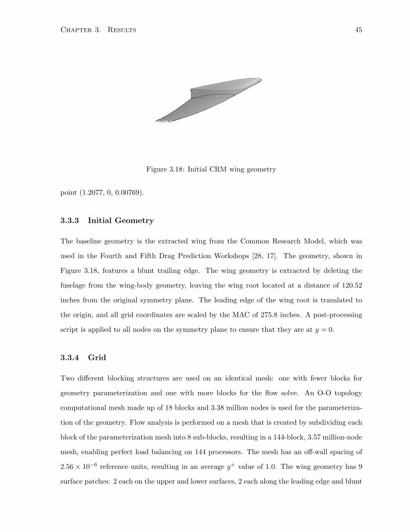
Chapter 3. Results 45
Figure 3.18: Initial CRM wing geometry
point (1.2077, 0, 0.00769).
3.3.3 Initial Geometry
The baseline geometry is the extracted wing from the Common Research Model, which was
used in the Fourth and Fifth Drag Prediction Workshops [28, 17]. The geometry, shown in
Figure 3.18, features a blunt trailing edge. The wing geometry is extracted by deleting the
fuselage from the wing-body geometry, leaving the wing root located at a distance of 120.52
inches from the original symmetry plane. The leading edge of the wing root is translated to
the origin, and all grid coordinates are scaled by the MAC of 275.8 inches. A post-processing
script is applied to all nodes on the symmetry plane to ensure that they are at y = 0.
3.3.4 Grid
Two different blocking structures are used on an identical mesh: one with fewer blocks for
geometry parameterization and one with more blocks for the flow solve. An O-O topology
computational mesh made up of 18 blocks and 3.38 million nodes is used for the parameteriza-
tion of the geometry. Flow analysis is performed on a mesh that is created by subdividing each
block of the parameterization mesh into 8 sub-blocks, resulting in a 144-block, 3.57 million-node
mesh, enabling perfect load balancing on 144 processors. The mesh has an off-wall spacing of
2.56 × 10⁻⁶ reference units, resulting in an average y+ value of 1.0. The wing geometry has 9
surface patches: 2 each on the upper and lower surfaces, 2 each along the leading edge and blunt

Chapter 3. Results 46
trailing edge, and one cap patch at the wing tip. The leading-edge patches (one for the inboard
section and one for the outboard) are required in order to match with the blunt trailing-edge
patches, and also serve as a method of better capturing the curvature of the leading edge.
In her Ph.D. thesis, Osusky [19] analyzed the initial and optimized geometries on a finer
mesh made up of 39.4× 10⁶ nodes and compared the results to those obtained on the 3.6× 10⁶
node mesh. When the analysis is done on the fine mesh, the pitching moment constraint is
violated, however the difference is less than 2%. The drag coefficients are 4 - 7% lower on
the fine mesh as compared to the coarse mesh. This analysis shows that the final geometry
produced reduces the drag relative to the initial geometry, even on a refined mesh.
3.3.5 Optimization Results
As in previous cases, the number of design variables used to parameterize the geometry is
varied to determine the effect this has on the final result. Figure 3.19 shows how the final
drag coefficient changes with the number of design variables. The data points represented by
red circles are parameterized using 5 spanwise control points on each surface patch, and then
the number of streamwise control points per patch is increased from 5 to 9. The data points
represented by blue squares are parameterized using 6 spanwise control points, with the same
pattern applied to the streamwise control points. The black triangle data points have 7 spanwise
control points. The lowest drag coefficient, 192.63 drag counts, is obtained with the coarsest
streamwise parameterization (5 control points per patch) and finest spanwise parameterization
(7 control points per patch). This is almost 20 drag counts lower than the initial drag coefficient
of 212 drag counts, which is a 9% reduction in drag. The drag coefficient decreases as the number
of spanwise control points used increases. As the number of spanwise control points increases,
there is more flexibility for the geometry to achieve an improved twist distribution. The drag
coefficient generally increases as the number of streamwise control points used increases. This
is contrary to the results seen by Carrier et al. [5], however their use of camber and twist
modifications, not section shape and twist modifications, means the problem was constrained
differently. The thickness constraint that requires the section shapes to maintain at least 25%
of the original thickness is imposed on the control points, not the surface itself. This means
that the thickness constraints vary slightly depending on the initial parameterization. It would

Chapter 3. Results 47
Number of Streamwise Control Points (Per Patch)
Fin
al D
rag
Co
effi
cien
t (C
ou
nts
)
5 6 7 8 9192.5
193
193.5
194
5 spanwise6 spanwise7 spanwi
Figure 3.19: CRM wing drag results - all parameterizations
be preferable to use nonlinear thickness constraints that enforce the thickness between surface
points, not between control points.
It is important to note that the optimizer is not fully converging for any of the cases. An
example of a typical convergence history is shown in Figure 3.20 for two cases: 5 streamwise and
5 spanwise control points per patch, and 5 streamwise and 7 spanwise control points per patch.
The optimality is reduced by roughly an order of magnitude overall, with the optimizer unable
to achieve deep convergence. With the number of surface patches required to fit this geometry,
the number of design variables ranges from 150 - 300, depending on the parameterization. The
high number of design variables is making it difficult for the optimizer to fully converge.
Figure 3.21 compares the initial and final lift distribution for the case with 5 streamwise
and 7 spanwise control points. The final distribution is closer to elliptical than the initial
distribution, showing that the optimizer has reduced the induced drag. Surface pressure coef-
ficient distributions and airfoil section shapes are shown in Figures 3.22 and 3.23, respectively.
These compare the initial and final results for the case with 5 streamwise and 7 spanwise con-
trol points. The pressure distributions show that the optimizer has changed the geometry to

Chapter 3. Results 48
Design Iteration
Op
tim
alit
y
0 10 20 30 40 50
0.0002
0.0004
0.0006
0.0008
0.001
0.0012
5 Spanwise Control Points7 Spanwise Control Points
Figure 3.20: Optimization convergence histories for CRM wing optimization - 5 streamwisecontrol points per patch
weaken or eliminate shock waves, in order to reduce wave drag. The airfoil shapes show that the
leading edge is becoming pointed near the wing tip. This feature is undesirable structurally and
aerodynamically at lower angles of attack, and can be avoided by using geometric constraints
or performing a multipoint optimization with cases at lower angles of attack.
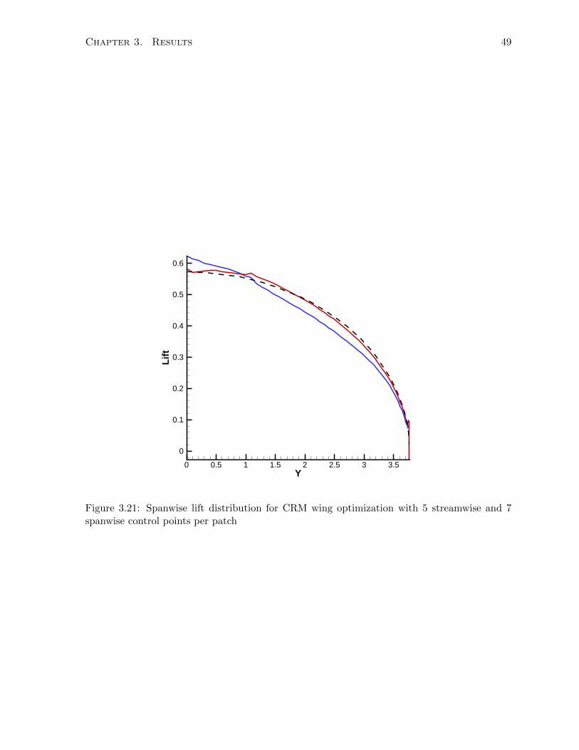
Chapter 3. Results 49
Y
Lif
t
0 0.5 1 1.5 2 2.5 3 3.5
0
0.1
0.2
0.3
0.4
0.5
0.6
Figure 3.21: Spanwise lift distribution for CRM wing optimization with 5 streamwise and 7spanwise control points per patch
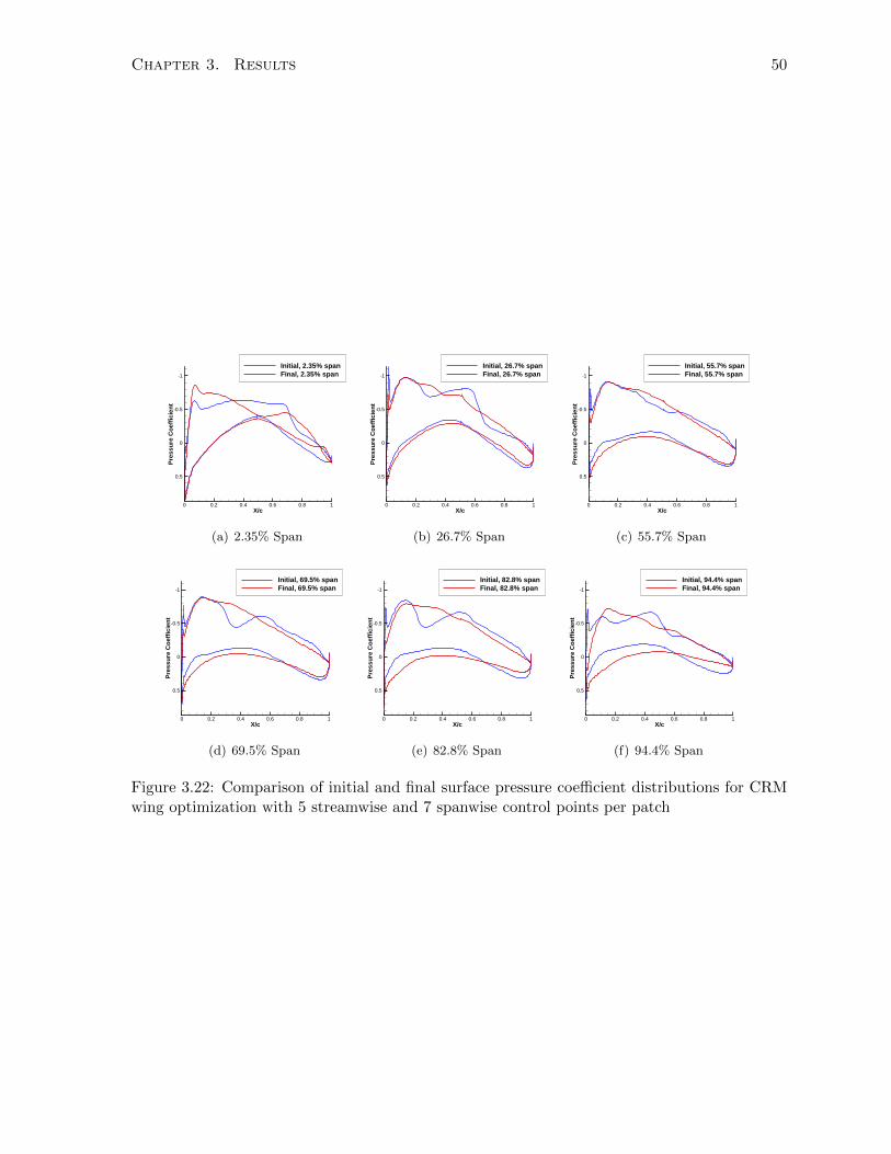
Chapter 3. Results 50
X/c
Pre
ssu
re C
oef
fici
ent
0 0.2 0.4 0.6 0.8 1
-1
-0.5
0
0.5
Initial, 2.35% spanFinal, 2.35% span
(a) 2.35% Span
X/c
Pre
ssu
re C
oef
fici
ent
0 0.2 0.4 0.6 0.8 1
-1
-0.5
0
0.5
Initial, 26.7% spanFinal, 26.7% span
(b) 26.7% Span
X/c
Pre
ssu
re C
oef
fici
ent
0 0.2 0.4 0.6 0.8 1
-1
-0.5
0
0.5
Initial, 55.7% spanFinal, 55.7% span
(c) 55.7% Span
X/c
Pre
ssu
re C
oef
fici
ent
0 0.2 0.4 0.6 0.8 1
-1
-0.5
0
0.5
Initial, 69.5% spanFinal, 69.5% span
(d) 69.5% Span
X/c
Pre
ssu
re C
oef
fici
ent
0 0.2 0.4 0.6 0.8 1
-1
-0.5
0
0.5
Initial, 82.8% spanFinal, 82.8% span
(e) 82.8% Span
X/c
Pre
ssu
re C
oef
fici
ent
0 0.2 0.4 0.6 0.8 1
-1
-0.5
0
0.5
Initial, 94.4% spanFinal, 94.4% span
(f) 94.4% Span
Figure 3.22: Comparison of initial and final surface pressure coefficient distributions for CRMwing optimization with 5 streamwise and 7 spanwise control points per patch

Chapter 3. Results 51
X
Z
0.5 1 1.5
-0.18
-0.16
-0.14
-0.12
-0.1
-0.08
-0.06
-0.04
-0.02
0
0.02
0.04
0.06
Initial, 2.35% SpanFinal, 2.35% Span
(a) 2.35% Span
X
Z
0.8 1 1.2 1.4 1.6 1.8
-0.04
-0.02
0
0.02
0.04
0.06
Initial, 26.7% SpanFinal, 26.7% Span
(b) 26.7% Span
X
Z
1.6 1.8 2 2.2
0.06
0.08
0.1
0.12
Initial, 55.7% SpanFinal, 55.7% Span
(c) 55.7% Span
X
Z
2 2.2 2.4 2.60.12
0.14
0.16
0.18
Initial, 69.5% SpanFinal, 69.5% Span
(d) 69.5% Span
X
Z
2.4 2.6 2.8
0.2
0.22
0.24
Initial, 82.8% SpanFinal, 82.8% Span
(e) 82.8% Span
X
Z
2.75 2.8 2.85 2.9 2.95 3 3.05 3.1
0.28
0.3
0.32
Initial, 94.4% SpanFinal, 94.4% Span
(f) 94.4% Span
Figure 3.23: Comparison of initial and final airfoil shapes for CRM wing optimization with 5streamwise and 7 spanwise control points per patch


Chapter 4
Conclusions and Recommendations
4.1 Conclusions
The objective of this thesis is to investigate the impact of the number of design variables on
three standard aerodynamic shape optimization test cases. The goal is to provide insight into
the impact of dimensionality on aerodynamic shape optimization. The three cases investigated
are:
1. drag minimization of a symmetrical two-dimensional airfoil in transonic inviscid flow,
subject to a thickness constraint that requires the airfoil to have thickness greater than
or equal to the NACA 0012 airfoil;
2. lift-constrained drag minimization through optimizing the twist distribution of a rectan-
gular wing with NACA 0012 sections in subsonic inviscid flow;
3. drag minimization through optimizing the twist distribution and section shapes of the
CRM blunt trailing edge wing in transonic turbulent flow subject to lift and pitching
moment constraints.
Due to the thickness constraint imposed for the first case, shock waves cannot be completely
eliminated. The optimizer thickens the airfoil near the trailing edge and is able to weaken the
shocks and move them aft. As the number of design variables increases, the general trend
shows a decrease in the final drag coefficient. However, the decrease is not strictly monotonic,
53
Chapter 4. Conclusions and Recommendations 54
and as the number of design variables increases, the optimizer is not able to achieve significant
reductions in optimality. As a result, the drag coefficient begins to increase. The lowest drag
coefficient is obtained with 9 design variables, and is reduced by 91% to 42 drag counts. The
results show that a finer parameterization is required to gain enough flexibility for the optimizer
to reduce the drag significantly; however this comes at a cost to optimization convergence.
For the second case, the optimization algorithm is able to produce a known result, the ellip-
tical spanwise lift distribution due to minimum induced drag for a planar wake. As the number
of spanwise control points increases, the drag coefficient decreases and the span efficiency factor
increases. However, the difference between the coarsest and finest parameterization is small.
The number of spanwise control points has no effect on the convergence of the optimizer, with
all cases able to converge to the required tolerance. The drag is reduced 3% and the span
efficiency factor is increased 3% from the initial geometry.
The third case introduces optimization based on the RANS equations. In contrast to the first
two cases, where most optimizations achieved the required optimality measure, the optimality is
not well converged for any of the parameterizations examined. Nevertheless, the drag coefficient
is consistently reduced. The number of streamwise and spanwise control points is varied from 5
to 9 in the streamwise direction and 5 to 7 in the spanwise direction, for a total of 15 different
parameterizations. The drag coefficient decreases as the number of spanwise control points
increases, and the lowest drag coefficient is seen with the coarsest streamwise parameterization
(5 control points per patch) and the finest spanwise parameterization (7 control points per
patch). The difference between the best and worst cases is 1.7 drag counts. For the best case,
the optimizer is able to achieve a drag reduction of 20 counts, or 9%, on the grid used for
optimization.
The optimization algorithm is able to achieve significant drag reductions in all three cases
studied. Valuable insight into the impact of dimensionality is gained, showing that increasing
the number of control points used to parameterize the geometry can provide greater flexibility
to the optimization algorithm. This flexibility can come at a cost to the convergence of the
optimization algorithm, whether that be due to an inability to reduce the optimality signif-
icantly, the increased geometric flexibility challenging the mesh movement algorithm, or the
unique aerodynamic shapes being unable to achieve converged flow solutions.

Chapter 4. Conclusions and Recommendations 55
4.2 Recommendations
For the first case, the number of design variables should be further increased beyond 11 to
see what impact increased dimensionality has. Other researchers who examined this test case
used as many as 64 control points (which would equate to 62 design variables). Many of the
final solutions are not in the grid converged region, so further study of the grid convergence of
the final solutions is required. For the second case, it would be preferable to analyze with a
coarser parameterization. Due to the grid created, the rectangular wing has 16 surface patches,
with each patch parameterized with 13 streamwise and 5 to 11 spanwise control points. This
is a relatively fine geometry parameterization. Using fewer surface patches, or decoupling the
number of design variables from the grid blocking, would allow a coarser parameterization to be
used. The optimizer produced a twist distribution with drastic changes in the twist angle near
the root, which is not desirable structurally. Imposing constraints to prevent this or performing
aerostructural optimization is recommended. For the third case, a complete grid convergence
study should be performed, particularly on the final optimized geometries.
The cases would benefit from analysis using free-form deformation (FFD), which would
allow for a larger number of geometric control points to be used while maintaining a manageable
number of design variables for the optimization algorithm. The first case would particularly
benefit from this treatment, as it shows a degradation in optimizer performance as the geometry
parameterization is refined. Chernukhin and Zingg [6] investigated the multimodality of several
types of problems, including an airfoil, wing, and blended-wing-body. It would be interesting
to investigate if any of the 3 cases show multimodality, and particularly if the number of design
variables could impact multimodality.


References
[1] O. Amoignon, J. Navratil, and J. Hradil. Study of parameterizations in the project
CEDESA. In 52nd AIAA Aerospace Sciences Meeting, number AIAA–2014–0570, National
Harbor, Maryland, January 2014.
[2] M. Andreoli, A. Janke, and J-A. Desideri. Free-form-deformation parameterization for
multilevel 3D shape optimization in aerodynamics. Technical report, Institut National de
Recherche en Informatique et en Automatique, 2003.
[3] F. Bisson, S. Nadarajah, and D. Shi-Dong. Adjoint-based aerodynamic optimization of
benchmark problems. In 52nd AIAA Aerospace Sciences Meeting, number AIAA–2014–
0412, National Harbor, Maryland, January 2014.
[4] H. P. Buckley and D. W. Zingg. On aerodynamic design through multipoint numerical op-
timization. In 49th AIAA Aerospace Sciences Meeting, number AIAA–2011–1244, Orlando,
Florida, January 2011.
[5] G. Carrier, D. Destarac, A. Dumont, M. Meheut, I. Salah El Din, J. Peter, and S. Ben
Khelil. Gradient-based aerodynamic optimization with the elsA software. In 52nd AIAA
Aerospace Sciences Meeting, number AIAA–2014–0568, National Harbor, Maryland, Jan-
uary 2014.
[6] O. Chernukhin and D. W. Zingg. Multimodality and global optimization in aerodynamic
design. AIAA Journal, 51(6):1342–1354, June 2013.
[7] Carl de Boor. A Practical Guide to Splines. Springer-Verlag Berlin and Heidelberg GmbH
and Co., 1978.
57
References 58
[8] P. E. Gill, W. Murray, and M. A. Saunders. SNOPT : An SQP algorithm for large-scale
constrained optimization. SIAM Review, 47(1):99–131, 2005.
[9] X. Han and D. W. Zingg. An adaptive geometry parametrization for aerodynamic shape
optimization. Journal of Optimization and Engineering, 15(1):69–91, March 2014.
[10] J. E. Hicken and D. W. Zingg. A parallel Newton-Krylov solver for the Euler equations
discretized using simultaneous approximation terms. AIAA Journal, 46(11):2773–2786,
November 2008.
[11] J. E. Hicken and D. W. Zingg. Aerodynamic optimization algorithm with integrated
geometry parameterization and mesh movement. AIAA Journal, 48(2):400–413, February
2010.
[12] J. E. Hicken and D. W. Zingg. Aerodynamic optimization algorithm with integrated
geometry parameterization and mesh movement. AIAA Journal, 48(2):400–413, 2010.
[13] J. Hoschek. Intrinsic parametrization for approximation. Computer Aided Geometric
Design, 5(1):27–31, June 1988.
[14] IATA. Vision 2050. Technical Report February, 2011.
[15] A. Jameson. Aerodynamic design via control theory. Journal of Scientific Computing,
3(3):233–260, 1988.
[16] N. Kumar, A. Diwakar, S. K. Attree, and S. Mittal. A method to carry out shape op-
timization with a large number of design variables. International Journal for Numerical
Methods in Fluids, 71:1494–1508, August 2013.
[17] D. W. Levy, K. R. Laflin, E. N. Tinoco, J. C. Vassberg, M. Mani, B. Rider, C. L. Rumsey,
R. A. Wahls, J. H. Morrison, O. P. Brodersen, S. Crippa, D. J. Mavriplis, and M. Mu-
rayama. Summary of data from the Fifth AIAA CFD Drag Prediction Workshop. In 51st
AIAA Aerospace Sciences Meeting and Aerospace Exposition, number AIAA–2013–0046,
Grapevine, Texas, United States, January 2013.

References 59
[18] J. A. Meijerink and H. A. van der Vorst. An iterative solution method for linear systems
of which the coefficient matrix is a symmetric m-matrix. Mathematics of Computation,
31(137):148–162, January 1977.
[19] L. Osusky. A numerical methodology for aerodynamic shape optimization in turbulent flow
enabling large geometric variation. PhD thesis, University of Toronto, 2013.
[20] L. Osusky and D. W. Zingg. A Novel Aerodynamic Shape Optimization Approach for
Three-Dimensional Turbulent Flows. In 50th AIAA Aerospace Sciences Meeting, number
AIAA–2012–0058, Nashville, Tennessee, United States, January 2012.
[21] L. Osusky and D. W. Zingg. Application of an efficient Newton-Krylov algorithm for
aerodynamic shape optimization based on the Reynolds-Averaged Navier-Stokes equations.
In 21st AIAA Computational Fluid Dynamics Conference, number AIAA–2013–2584, San
Diego, California, United States, June 2013.
[22] M. Osusky, J. E. Hicken, and D. W. Zingg. A parallel Newton-Krylov-Schur flow solver
for the Navier-Stokes equations using the SBP-SAT approach. In 48th AIAA Aerospace
Sciences Meeting and Aerospace Exposition, number AIAA–2010–116, Orlando, Florida,
United States, January 2010.
[23] K. Ou, A. Jameson, and J. C. Vassberg. Airfoils supporting non-unique transonic solutions
for unsteady viscous flows. In 7th AIAA Theoretical Fluid Mechanics Conference, number
AIAA–2014–2927, June 2014.
[24] O. Pironneau. Optimal shape design for elliptic systems. Springer-Verlag, 1983.
[25] P. Thokala and J. R. R. A. Martins. Variable-complexity optimization applied to airfoil
design. Engineering Optimization, 39(3):271–286, April 2007.
[26] A. H. Truong, C. A. Oldfield, and D. W. Zingg. Mesh movement for a discrete adjoint
Newton-Krylov algorithm for aerodynamic optimization. AIAA Journal, 46(7):1695–1704,
July 2008.
[27] J. C. Vassberg, N. A. Harrison, D. L. Roma., and A. Jameson. A systematic study on the
impact of dimensionality for a two-dimensional aerodynamic optimization model problem.
References 60
In 29th AIAA Applied Aerodynamics Conference, number AIAA–2011–3176, pages 1–19,
Honolulu, Hawaii, June 2011.
[28] J. C. Vassberg, E. N. Tinoco, M. Mani, B. Rider, T. Zickuhr, D. W. Levy, O. P. Broder-
sen, B. Eisfeld, S. Crippa, R. A. Wahls, J. H. Morrison, D. J. Mavriplis, and M. Mu-
rayama. Summary of the fourth AIAA CFD Drag Prediction Workshop. In 28th AIAA
Applied Aerodynamics Conference, number AIAA–2010–4547, Chicago, Illinois, United
States, June 2010.
[29] D. W. Zingg, M. Nemec, and T. H. Pulliam. A comparative evaluation of genetic and
gradient-based algorithms applied to aerodynamic optimization. REMN, 48(2):103–126,
February 2008. (invited paper in a special issue on adjoint-based shape design in Revue
Europeenne de Mecanique Numerique - European Journal of Computational Mechanics).