Durham E-Theses

Application of Modern Techniques in Crystallographic

Software Development

GILDEA, RICHARD,JAMES

How to cite:

GILDEA, RICHARD,JAMES (2011) Application of Modern Techniques in Crystallographic Software

Development, Durham theses, Durham University. Available at Durham E-Theses Online:http://etheses.dur.ac.uk/3332/

Use policy

The full-text may be used and/or reproduced, and given to third parties in any format or medium, without prior permission orcharge, for personal research or study, educational, or not-for-pro�t purposes provided that:

• a full bibliographic reference is made to the original source

• a link is made to the metadata record in Durham E-Theses

• the full-text is not changed in any way

The full-text must not be sold in any format or medium without the formal permission of the copyright holders.

Please consult the full Durham E-Theses policy for further details.

Academic Support O�ce, Durham University, University O�ce, Old Elvet, Durham DH1 3HPe-mail: e-theses.admin@dur.ac.uk Tel: +44 0191 334 6107

http://etheses.dur.ac.uk

2

Application of Modern

Techniques in Crystallographic

Software Development

Richard J. Gildea

Department of Chemistry

Durham University

A thesis submitted for the degree of

Doctor of Philosophy

March 2011

Declaration

The work described herein was carried out at Durham University be-

tween October 2007 and March 2011 under the supervision of Professor

Judith A.K. Howard. Unless otherwise stated all the work is my own

and has not been submitted previously for a degree at this or any other

university.

Richard J. Gildea

The copyright of this thesis rests with the author. No quotation from it

should be published without the prior written consent and information

derived from it should be acknowledged.

Acknowledgements

I would like to start by giving thanks to my supervisor, Professor Judith

Howard, for having the trust in allowing me the freedom to explore

those areas of the project I found most interesting, and for providing

support and giving me the opportunity to visit several international

conferences during the course of my PhD.

I am hugely grateful to all of the Olex2 team: Luc Bourhis, Oleg

Dolomanov and Horst Puschmann. You are a fantastic group of people

to work with, and my PhD would not have been anywhere near as much

fun without any one of you.

Luc Bourhis for his patience in spending so many hours explaining

mathematical and crystallographic concepts in detail, and for putting

up with all my questions about programming. Oleg Dolomanov for the

time spent donating his crystallographic and programming expertise

and countless hours spent debugging code and compiler errors. Thanks

for those beers in Istanbul, and the innumerable “last” pints in the

Market Tavern. Horst Puschmann for his constantly positive attitude,

for putting up with me sitting next to him for three and a half years,

and for counting pixels.

I would like to thank my parents for their support and encouragement

throughout my education and for pushing me to reach my full potential.

Finally, I must thank all the friends I have made during my time in

Durham, especially those with whom I have lived with throughout the

years, you have made my stay in Durham all the more enjoyable.

Abstract

This thesis describes contributions made as part of the EPSRC-funded

project Age Concern: Crystallographic Software for the Future. Work

has been done in various areas of small molecule crystallographic soft-

ware development, both within the smtbx (Small Molecule Toolbox)

and the Olex2 software.

Chapter 2 details the work that was done towards the smtbx-based re-

finement that was developed as part of the “Age Concern” project.

A framework was created enabling the inclusion of observations of

restraint in the refinement, and new restraints on geometry and

anisotropic displacement parameters were added. Refinement of

(pseudo-)merohedrally twinned structures was implemented.

In Chapter 3 a description of the determination of absolute structure

by various methods is given. The methods of Hooft et al. [2008] and

Flack [1983] have been implemented, and a quantitative comparison

made between the two methods.

Chapter 4 discusses the method of van der Sluis and Spek [1990] for the

refinement of structures containing severely disordered regions. This

method has been implemented and a modification designed to give

improved results when one or more low angle reflections are missing is

proposed and tested, and shown to be beneficial.

Chapter 5 introduces a new module, iotbx.cif, which has been added

to the cctbx (Computational Crystallography Toolbox), providing a

comprehensive set of tools for the manipulation of Crystallographic

Information Files (CIFs).

Contents

Contents iv

List of Figures vii

Nomenclature x

1 Introduction 1

1.1 Age Concern: Crystallographic Software for the Future . . . . . . . 1

1.2 Olex2 . . . . . . . . . . . . . . . . . . . . . . . . . . . . . . . . . . 3

1.3 Computational Crystallographic Toolbox . . . . . . . . . . . . . . . 4

1.4 Small Molecule Toolbox . . . . . . . . . . . . . . . . . . . . . . . . 5

1.4.1 Outline . . . . . . . . . . . . . . . . . . . . . . . . . . . . . 5

2 Least Squares Refinement 6

2.1 Restrained Least Squares Refinement . . . . . . . . . . . . . . . . . 7

2.1.1 Geometry Restraints . . . . . . . . . . . . . . . . . . . . . . 9

2.1.1.1 Restraints involving symmetry . . . . . . . . . . . 10

2.1.1.2 Bond similarity restraint . . . . . . . . . . . . . . . 10

2.1.2 Restraints on Atomic Displacement Parameters . . . . . . . 11

2.1.2.1 Rigid-bond restraint . . . . . . . . . . . . . . . . . 12

2.1.2.2 ADP similarity restraint . . . . . . . . . . . . . . . 13

2.1.2.3 Isotropic ADP restraint . . . . . . . . . . . . . . . 14

2.1.3 Implementation . . . . . . . . . . . . . . . . . . . . . . . . . 15

2.1.4 Applications . . . . . . . . . . . . . . . . . . . . . . . . . . . 19

2.1.4.1 Bond similarity restraint . . . . . . . . . . . . . . . 19

iv

CONTENTS

2.1.4.2 ADP similarity restraints . . . . . . . . . . . . . . 20

2.2 Twinning . . . . . . . . . . . . . . . . . . . . . . . . . . . . . . . . 22

2.2.1 Testing . . . . . . . . . . . . . . . . . . . . . . . . . . . . . . 25

2.3 Errors on derived parameters . . . . . . . . . . . . . . . . . . . . . 27

2.3.1 Symmetry . . . . . . . . . . . . . . . . . . . . . . . . . . . . 29

2.3.2 Discussion . . . . . . . . . . . . . . . . . . . . . . . . . . . . 30

3 Reflection Statistics 32

3.1 Absolute Structure . . . . . . . . . . . . . . . . . . . . . . . . . . . 32

3.1.1 Anomalous Scattering . . . . . . . . . . . . . . . . . . . . . 32

3.1.2 Hamilton’s Ratio Test . . . . . . . . . . . . . . . . . . . . . 34

3.1.3 Rogers η Parameter . . . . . . . . . . . . . . . . . . . . . . . 34

3.1.4 Flack x Parameter . . . . . . . . . . . . . . . . . . . . . . . 34

3.1.5 Hooft y Parameter . . . . . . . . . . . . . . . . . . . . . . . 36

3.1.5.1 Treatment of Outliers . . . . . . . . . . . . . . . . 40

3.1.5.2 Probability plots . . . . . . . . . . . . . . . . . . . 40

3.1.5.3 Student’s t-distribution . . . . . . . . . . . . . . . 42

3.1.5.4 Applications . . . . . . . . . . . . . . . . . . . . . 44

3.1.5.5 Results . . . . . . . . . . . . . . . . . . . . . . . . 45

3.1.6 Implementation . . . . . . . . . . . . . . . . . . . . . . . . . 46

3.2 Reflection Statistics in Olex2 . . . . . . . . . . . . . . . . . . . . . . 48

3.2.1 Cumulative Intensity Distribution . . . . . . . . . . . . . . . 49

3.2.2 Fo vs. Fc Plot . . . . . . . . . . . . . . . . . . . . . . . . . . 50

3.2.3 Data Completeness . . . . . . . . . . . . . . . . . . . . . . . 51

4 A New Solvent Masking Procedure 54

4.1 Introduction . . . . . . . . . . . . . . . . . . . . . . . . . . . . . . . 54

4.2 Theory . . . . . . . . . . . . . . . . . . . . . . . . . . . . . . . . . . 57

4.2.1 Refinement . . . . . . . . . . . . . . . . . . . . . . . . . . . 58

4.2.2 Incomplete Data . . . . . . . . . . . . . . . . . . . . . . . . 59

4.2.3 Twinned Data . . . . . . . . . . . . . . . . . . . . . . . . . . 61

4.2.4 Standard Uncertainties . . . . . . . . . . . . . . . . . . . . . 61

4.3 Method . . . . . . . . . . . . . . . . . . . . . . . . . . . . . . . . . 62

v

CONTENTS

4.4 Implementation . . . . . . . . . . . . . . . . . . . . . . . . . . . . . 63

4.4.1 Computational Crystallography Toolbox . . . . . . . . . . . 63

4.4.2 Olex2 . . . . . . . . . . . . . . . . . . . . . . . . . . . . . . 64

4.5 Test Structures . . . . . . . . . . . . . . . . . . . . . . . . . . . . . 64

4.6 Applications . . . . . . . . . . . . . . . . . . . . . . . . . . . . . . . 68

4.7 Discussion . . . . . . . . . . . . . . . . . . . . . . . . . . . . . . . . 69

5 The Crystallographic Information Framework (CIF) 74

5.1 iotbx.cif . . . . . . . . . . . . . . . . . . . . . . . . . . . . . . . . . 74

5.1.1 Introduction . . . . . . . . . . . . . . . . . . . . . . . . . . . 74

5.1.2 Using iotbx.cif . . . . . . . . . . . . . . . . . . . . . . . . . . 76

5.1.2.1 CIF output . . . . . . . . . . . . . . . . . . . . . . 79

5.1.3 Validation of CIFs against data dictionaries . . . . . . . . . 80

5.1.4 Interconversion with cctbx crystallographic objects . . . . . 81

5.1.5 Performance . . . . . . . . . . . . . . . . . . . . . . . . . . . 81

5.1.6 Common CIF syntax errors and error recovery . . . . . . . . 83

5.1.7 Discussion . . . . . . . . . . . . . . . . . . . . . . . . . . . . 86

5.2 CIF as a publication and archiving format . . . . . . . . . . . . . . 86

6 Concluding Remarks 88

A Absolute Structure Results 91

B CIF Grammar 110

C Additional Information 119

D Supplementary Electronic Materials 122

D.1 cctbx source code . . . . . . . . . . . . . . . . . . . . . . . . . . . . 122

D.2 Olex2 binaries . . . . . . . . . . . . . . . . . . . . . . . . . . . . . . 124

References 126

vi

List of Figures

2.1 Flow diagram illustrating the steps taken when building up the

normal equations. . . . . . . . . . . . . . . . . . . . . . . . . . . . . 16

2.2 Demonstration of the effective use of ADP similarity restraints. . . 21

2.3 Flow diagram illustrating the steps taken when building up the

normal equations taking twinning into account. . . . . . . . . . . . 26

3.1 The probability density function of pu(γ) with and without rejection

of 348 (23%) Bijvoet differences outliers. With rejection of outliers

the probability density is shifted towards γ = 0, giving G = 1.2(11)

compared to G = 1.5(10) without such outlier rejection. The prob-

ability plot slopes were 0.544 and 0.754 respectively. . . . . . . . . . 41

3.2 A comparison of a normal distribution and Student’s t fit of the

same set of Bijvoet differences. . . . . . . . . . . . . . . . . . . . . . 43

3.3 The probability density function of pu(γ) for two structures with

G = 1.6(7) and 1.02(2) respectively. . . . . . . . . . . . . . . . . . . 44

3.4 A plot of the Flack x parameter against the Hooft y parameter

calculated using the Student’s t distribution for the error model.

The straight dashed line is the total least squares line of best fit

of the data, y = 0.985x + 0.007. The grey error bars indicate the

standard uncertainty in the calculated values of the Flack x and

Hooft y parameters respectively. . . . . . . . . . . . . . . . . . . . . 47

3.5 An example of a Bijvoet differences scatter plot as displayed in Olex2. 49

3.6 An example of the presence of twinning being indicated by the cu-

mulative intensity distribution. . . . . . . . . . . . . . . . . . . . . 50

vii

LIST OF FIGURES

3.7 The effects of twinning and extinction on a plot of Fo vs. Fc. The

line y = x is plotted as a dashed line. . . . . . . . . . . . . . . . . . 52

3.8 A plot of data completeness in resolution shells. . . . . . . . . . . . 53

4.1 New structures deposited with CSD per year that are disordered,

or have used the SQUEEZE routine. . . . . . . . . . . . . . . . . . 55

4.2 An image of the Chicago skyline (a) and its Fourier transform (d);

(b) is the image reconstructed after application of a low-pass filter

to the Fourier transform (e); (c) is the image reconstructed after

application of a high-pass filter to the Fourier transform (f). Fourier

transforms calculated using the FTL-SE software [JCrystalSoft, 2010]. 60

4.3 The completeness in resolution shells for compound I after approx-

imately 5% of the reflections were discarded at random. . . . . . . . 66

4.4 The amplitudes of three ‘floating’ missing structure factors at each

iteration of the solvent masking procedure. The lightly dashed hor-

izontal lines indicate the ‘true’ amplitudes. . . . . . . . . . . . . . . 66

4.5 The view of the unit cell down the c-axis for compound VII. The

peaks in the difference electron density are displayed as transparent

light-brown spheres. . . . . . . . . . . . . . . . . . . . . . . . . . . . 70

4.6 Two alternate views of electron density map for F diff for compound

VII. . . . . . . . . . . . . . . . . . . . . . . . . . . . . . . . . . . . 71

5.1 A simplified rule dependency graph for the CIF grammar. . . . . . 77

viii

Nomenclature

Roman Symbols

At The transpose of the matrix A.

h A column vector of the Miller indices of a Bragg reflection.

ht The transpose of the column vector h (i.e. a row vector).

F (h) The complex structure factor associated with Miller indices h.

Greek Symbols

σ Standard deviation or uncertainty

Acronyms

ADP Anisotropic Displacement Parameter

ASCII American Standard Code for Information Interchange

CBF Crystallography Binary Format

cctbx Computational Crystallography Toolbox

CIF Crystallographic Information File (Framework)

COD Crystallography Open Database

CSD Cambridge Structural Database

EPSRC Engineering and Physical Sciences Research Council

ix

LIST OF FIGURES

GUI Graphical User Interface

HTML HyperText Markup Language

IUCr International Union of Crystallography

smtbx Small Molecule Toolbox

x

Chapter 1

Introduction

1.1 Age Concern: Crystallographic Software for

the Future

The work described in this thesis is part of a larger software project between

groups in Durham and Oxford funded by the EPSRC of the UK1, with the title

Age Concern: Crystallographic Software for the Future. The background to this

project, and also the aims and objectives as outlined in the grant proposal, are

described in detail by Howard and Watkin [2009] and Dolomanov et al. [2009b].

They highlight that whilst in previous decades (1960s, 1970s, 1980s) there was

healthy competition amongst a wide variety of actively developed crystallographic

systems, in recent years only relatively few are still under active development and

commonly used within the small molecule community. They noted that many

of the authors of significant programs are approaching retirement, with no clear

indication of who would take their place, either through continued development of

the existing programs, or by development of a new generation of crystallographic

software.

Much of the computer code currently used in small molecule crystallography

has its foundations in code written up to 40 years ago, using older programming

languages and techniques. Consequently, it is frequently difficult for such code

to be extended significantly, or reused in a different context, in particular by

1EPSRC Grant EP/C536274/1

1

developers other than the original authors. Nonetheless, there is a huge amount

of knowledge and experience that is coded within these programs, which any new

software should strive to incorporate.

In contrast to the small molecule crystallographic community, there currently

exist two substantial multi-author efforts within macromolecular crystallography

that coordinate the software developments of multiple groups of programmers,

namely CCP4 [Potterton et al., 2004] and PHENIX [Adams et al., 2010].

In view of the massive advances both in computer hardware and programming

techniques since those long-standing programs were first conceived, it was proposed

to provide a new crystallographic software framework implemented in modern

programming languages and written in a style designed to maximise extensibility

and reusability of code. In addition to providing much of the functionality of the

software in common use, this new framework should ensure that new ideas and

algorithms in crystallographic computing can be developed rapidly and effectively,

and made available to the wider crystallographic community with minimal effort.

A reference application would be developed which would at the same time serve

as a test-application for the development of the newly created framework, whilst

also providing the crystallographic community with a fully functional, single crys-

tal refinement application with unprecedented functionality, flexibility, customis-

ability and extensibility.

It was decided that the crystallographic software framework would be based

upon the pre-existing cctbx (Computational Crystallography Toolbox) which is

described in §1.3. A new small molecule toolbox, the smtbx, would provide a set

of algorithms dedicated to small molecule crystallography, whilst tools developed

in the course of the project that are more generally applicable to the whole of

crystallography would be added to the cctbx itself, thus contributing back to the

wider crystallographic software community as a whole.

The reference application mentioned in the proposal became the software Olex2,

which would provide access to the new tools developed within the smtbx as they

became available.

2

1.2 Olex2

A more comprehensive overview of the Olex2 software and its design and im-

plementation is given by Dolomanov et al. [2009a]. The core of the program is

written using the C++ programming language and is highly optimised for excel-

lent graphical performance. The program is designed as a set of libraries which can

be re-used to build applications with minimal dependencies. Separate libraries are

concerned with core functionality, crystallographic operations, input/output and

graphical display. As a result, a command line version of the Olex2 executable

exists in addition to the graphical user interface (GUI). The graphical display of

the model uses the OpenGL [Khronos Group] library. Extended functionality of

the Olex2 core is achieved in two ways: through the use of a built-in macro lan-

guage; or through the provision of an embedded Python interpreter. The control

panel section of the GUI is written using extended HTML which is displayed us-

ing wxWidgets. This provides a set of GUI controls which support event-driven

execution, allowing the creation of a clearly laid out and easy-to-follow workflow

path.

Much of the overall workflow (especially with regard to structure solution,

refinement, and report preparation stages) is written in Python/HTML. Functions

or macros provided by the Olex2 core can be accessed either through the command

console, which is part of the OpenGL window, or through functionality provided

by the GUI.

The Python layer allows the integration of the cctbx (Computational Crys-

tallography Toolbox) and its subpackage, the smtbx (Small Molecule Toolbox).

This vastly extends the functionality available through Olex2, including tools for

structure solution and refinement.

In addition to the structure solution and refinement methods provided through

the smtbx, Olex2 also supports the SHELX suite of solution and refinement pro-

grams [Sheldrick, 2008]. Plugins have also been developed by interested users

providing access to a range of external programs including PLATON [Spek, 2003],

the structure solution program SUPERFLIP [Palatinus and Chapuis, 2007] and

the SIR9x-SIR20xx range of structure solution programs [Burla et al., 2007].

The latest installers for Windows, Mac and Linux are included on the DVD

3

accompanying this thesis. Details regarding their installation can be found in

Appendix D.

1.3 Computational Crystallographic Toolbox

The Computational Crystallographic Toolbox (cctbx) is an open source code li-

brary originally developed as the open source component of the PHENIX system

[Adams et al., 2010] for macromolecular structure determination. It features an

object-oriented, highly modular design, which encourages code reuse across many

different applications. The cctbx is written using a combination of two modern

programming languages, Python [Python Software Foundation] and C++, which

provides the flexibility of using an interpreted language (Python) at the same time

as the performance benefits gained through using a statically typed, compiled lan-

guage (C++). Python bindings for C++ code are written using the Boost.Python

library. The cctbx code is extremely portable, and is known to compile on a

large range of hardware and platforms. The writing of regression tests is actively

encouraged, contributing to the stability of the cctbx.

The foundation of the cctbx is the scitbx module, which provides a large number

of tools for general scientific computing. Built upon this is the cctbx module, a

set of libraries for general crystallographic applications. The iotbx (input/output

toolbox) provides libraries for reading and writing most common crystallographic

formats. For an in-depth discussion of the design of the cctbx the reader is referred

to Grosse-Kunstleve et al. [2002] and the several cctbx articles in the newsletters

of the IUCr Commission on Crystallographic Computing, in particular the very

first one [Grosse-Kunstleve and Adams, 2003].

The latest cctbx source code bundles are included on the DVD accompanying

this thesis. Details regarding their extraction and compilation can be found in

Appendix D.

4

1.4 Small Molecule Toolbox

The Small Molecule Toolbox (smtbx) is an extension of the cctbx with a partic-

ular emphasis on the provision of algorithms and tools that are specific to small

molecule crystallography. Currently it provides ab initio structure solution using

the charge flipping algorithm [Oszlanyi and Suto, 2008], full matrix least squares

refinement of crystal structures with constraints and restraints on parameters, an

implementation of the BYPASS algorithm for treating severely disordered solvent

in structure refinement [van der Sluis and Spek, 1990], and tools for the determi-

nation of absolute structure.

1.4.1 Outline

Chapter 1 describes work carried out as part of the development of the least squares

refinement program, smtbx-refine. §2.1 describes the framework that was imple-

mented to allow the inclusion of restraints on anisotropic displacement parameters

and geometry in the refinement. The addition of refinement of (pseudo)merohedrally

twinned crystal structures is described in §2.2, and §2.3 details the calculation of

errors on derived parameters.

§3.1 contains a discussion of the various methods for the determination of

absolute structure, along with a description of the implementation of two of those

methods within the smtbx. A quantitative comparison is made between the two

methods. A description of the various graphs for the analysis of reflection statistics

that have been implemented using the cctbx is given in §3.2. The graphs are made

available using the new graph plotting tool implemented in Olex2.

Chapter 4 contains a description of the procedure of van der Sluis and Spek

[1990] for dealing with severely disordered solvent. The procedure has been imple-

mented within the smtbx and a modification is proposed in §4.2.2 that is intended

to give improved results for the procedure when some low angle data are missing.

Several test cases and applications of the procedure are given.

A new module has been added to the cctbx providing extensive support for the

Crystallographic Information Framework (CIF); a description of the implementa-

tion and capabilities of the new module is given in Chapter 5.

5

Chapter 2

Least Squares Refinement

A crystal structure X-ray diffraction experiment yields a set of intensities of

diffracted X-ray beams which contain information about the electron density dis-

tribution in the unit cell. The Fourier transform relationship between the electron

density, ρ(x), and the structure factors, F (h), is given by:

ρ(x) = V −1∑h

|F (h)| exp(iφh) exp(−2πih · x) (2.1)

and

F (h) =

∫cell

ρ(x) exp(2πih · x) dx, (2.2)

where h is a column vector of the Miller indices for a Bragg reflection.

The electron density is usually interpreted in terms of an atomic model and

the structure factors can then be calculated according to

F (h) 'atoms∑j

fjT (h) exp(2πih · x), (2.3)

where fj is the scattering factor calculated for an atom at zero Kelvin and x =

(x, y, z) are the atomic coordinates. The Debye-Waller factor, T (h), is given by

T (h) = exp(−2π2htU∗h), (2.4)

where U∗ is a symmetric second-rank tensor whose elements are dimensionless

6

mean-square displacements. U∗ is one of several definitions of the anisotropic

displacement parameters (ADPs) [Grosse-Kunstleve and Adams, 2002].

Once an atomic model is proposed, the parameters of the model can be varied

in order to obtain the best possible model given the experimental data. In small

molecule crystallography, this is usually achieved by least squares refinement of

the structural parameters.

2.1 Restrained Least Squares Refinement

A small molecule structure refinement typically minimises the weighted least squares

function

L =∑h

wh(Yobs(h)− kYcalc(h))2 (2.5)

where Yobs are the X-ray observations, either Fobs or F 2obs, and Ycalc are similarly

|Fcalc| or |Fcalc|2 where Fcalc are the structure factors calculated from the current

structure model according to equation 2.3, and k is an overall scale factor that

places Ycalc on the same scale as Yobs. Each observation is given an appropriate

weight, wh, based on the reliability of the measurement. These may be pure

statistical weights, w = 1/σ2(Yobs), where σ is the estimated standard deviation

of the Yobs, although more complex weighting schemes are usually used.

Since the minimisation function introduced above is not linear, the minimisa-

tion is non-linear least squares, which requires that we calculate the gradients of

Ycalc with respect to each parameter. For a small molecule structure with a high

data to parameter ratio, such unconstrained minimisation as defined by equation

2.5 may well be sufficient. However, as the structure becomes larger, or the data

to parameter ratio worsens, unconstrained minimisation may not be well-behaved,

or result in some questionable parameter values. These X-ray observations can be

supplemented with the use of ‘observations of restraint’, as suggested by Waser

[1963], where additional information, such as target values for bond lengths, angles

etc. is included in the minimisation. This now gives the minimisation function

L =∑h

wh(Yobs(h)− kYcalc(h))2 +∑

restraints

w(Tobs − Tcalc)2 (2.6)

7

where Tobs is the target value for our restraint, and Tcalc is the value of the target

function calculated using the current model (see, for example Giacovazzo et al.

[2002]; Watkin [2008]). With the use of appropriate weighting of the restraints the

minimisation is gently pushed towards giving a chemically sensible and hopefully

correct structure.

Using the notation of Watkin [2008], the observational least squares equations

can be written

W ·A · δx = W ·∆Y, (2.7)

with the weight matrix and the vector of residuals, ∆Y, where each row is given

by Yobs(h)− kYcalc(h). The elements of the matrix of derivatives, A, are given by

Aij =∂Yc(hi)

∂xi. (2.8)

The shifts, δx, in the values of the refined parameters are obtained via the

solution of the normal equations,

AT ·W ·A · δx = AT ·W ·∆Y. (2.9)

If we allow the repameterisation of the model by use of constraints, the vector

of parameters, x is expressed as a function of a smaller vector of parameters, y,

in a non-linear fashion. The linearisation of that relationship reads

δx = Mδy (2.10)

where M is the matrix of constraint, usually known to mathematicians as the

Jacobian matrix of the transformation y→ x.

Since the normal matrix, AT ·W · A is symmetric, it can be inverted using

the Cholesky method. A naıve approach to solving these equations would start

by first of all constructing the matrix of derivatives, A. This is not feasible, since

the design matrix is of size m × nx, for m observations, and nx crystallographic

parameters. In a typical small molecule crystal structure determination, the data

to parameter ratio, m/nx is typically in the range 10−30. In contrast, the normal

matrix, AT ·W ·A is symmetric, with dimensions nx×nx. With the common use

8

of constraints, particularly with respect to those on the parameters of hydrogen

atoms, the ratio nx/ny can be as large as 2, meaning that the most efficient, both

in terms of storage and floating point operations, would in fact be to construct

directly the normal matrix for the independent parameters, MTAT ·W ·AM.

Whilst the part of the design matrix derived from the observations is relatively

dense, that coming from the equations of restraint is sparse, with each restraint

typically only involving a few crystallographic parameters. Therefore, it is now

feasible to compute and store the design matrix for the restraints independently,

and then use sparse matrix techniques to compute the contribution of the restraints

to the overall normal equations.

It would be desirable to place the weights of the restraints on the same scale as

the typical residual, such that a restraint will have a similar strength for the same

weight in different structures. Giacovazzo et al. [2002] suggest the normalization

factor

wrestraints =∑h

wh(Yobs(h)− kYcalc(h))2/ (m− ny) , (2.11)

where for m observations and ny independent parameters. This is better known

as the square of the goodness of fit, χ2. Ths normalising factor also allows the

restraints to have greater influence when the fit of the model to the data is poor

(and the goodness of fit is greater than unity), whilst their influence lessens as the

fit improves [SHELX manual, Sheldrick, 1997].

2.1.1 Geometry Restraints

Possible restraints on the stereochemistry or geometry of atomic positions include

restraints on bond distances, angles and dihedral angles, chiral volume and pla-

narity. These restraints are used extensively in macromolecular crystallography,

and hence were already implemented within the cctbx as part of the macromolec-

ular refinement program phenix.refine [Adams et al., 2010]. With the exception

of the bond distance restraint, these restraints were not able to accept symmetry

equivalent atoms. Since this is more frequently required in small molecule crys-

tallography, these restraints have now been extended to allow for symmetry. We

have also implemented other restraints commonly used in small molecule struc-

9

ture refinement, such as a bond similarity restraint, and restraints on anisotropic

displacement parameters (ADPs) including restraints based on Hirshfeld’s ‘rigid-

bond’ test [Hirshfeld, 1976], similarity restraints and isotropic ADP restraints.

2.1.1.1 Restraints involving symmetry

Given a restraint, f(x), involving a site x which is outside the asymmetric unit

and which is related to the site y within the asymmetric unit by some symmetry

transformation M , such that x = My, the gradient is transformed as

∇y (f (x)) = MT∇x (f (x))

= M−1∇x (f (My)) (2.12)

since M is a space group symmetry operation and is therefore an orthogonal trans-

formation (i.e. one which preserves distances and angles), which means that,

MT = M−1.

2.1.1.2 Bond similarity restraint

The distances between two or more atom pairs are restrained to be equal by

minimising the weighted variance of the distances, where the least squares residual,

R, is defined as the population variance biased estimator

R(r1, ..., rn) =

∑ni=1wi(ri − 〈r〉)2∑n

i=1wi. (2.13)

As discussed above, since our minimisation is non-linear, we need the derivatives of

the residuals with respect to the least squares parameters. It is easier to compute

the derivatives by using the alternative form of the residual

R =⟨r2⟩− 〈r〉2

=

∑ni=1wir

2i∑n

i=1 wi−(∑n

i=1wiri∑ni=1 wi

)2

. (2.14)

10

The derivative of the residual with respect to a distance rj is then

∂R

∂rj=

2wjrj∑ni=1 wi

− 2wj∑n

i=1 wiri(∑n

i=1wi)2

=2wj∑ni=1 wi

(rj − 〈r〉). (2.15)

Given that

rj = u12 ,

where for a pair of atoms, a and b,

u = (xa − xb)2 + (ya − yb)2 + (za − zb)2,

the derivative of rj with respect to the Cartesian coordinate xa is then

∂rj∂xa

=∂rj∂u

∂u

∂xa=

(xa − xb)rj

. (2.16)

Therefore, the derivative of the residual with respect to xa is

∂R

∂xa=∂R

∂rj

∂rj∂xa

=2wj(rj − 〈r〉)(xa − xb)

rj∑n

i=1wi. (2.17)

2.1.2 Restraints on Atomic Displacement Parameters

There appears to be very little in the literature with regard to restraints on ADPs,

and in particular the details of their implementation in refinement programs. It

was therefore necessary to devise our formulae for the equations of restraints and

derive their gradients with respect to the least squares parameters. The analytical

gradients were confirmed to be correct by testing against gradients determined

by the finite differences method. The residuals were also tested for frame invari-

ance (i.e. for a given Ucart, the least squares residual should be unchanged after

transformation of Ucart by an arbitrary rotation matrix).

11

2.1.2.1 Rigid-bond restraint

In a ‘rigid-bond’ restraint the components of the anisotropic displacement param-

eters of two atoms in the direction of the vector connecting those two atoms are

restrained to be equal. This corresponds to Hirshfeld’s ‘rigid-bond’ test [Hirshfeld,

1976] for testing whether anisotropic displacement parameters are physically rea-

sonable [see SHELX manual, DELU restraint, Sheldrick, 1997] and is in general

appropriate for bonded and 1,3-separated pairs of atoms and should hold true for

most covalently bonded systems.

We therefore minimise the mean square displacement of the atoms in the di-

rection of the bond. The weighted least squares residual is then

R = w(z2A,B − z2

B,A)2, (2.18)

where in the Cartesian coordinate system the mean square displacement of atom

A along the vector−→AB, z2

A,B, is given by

z2A,B =

rTUcart,Ar

‖r‖2, (2.19)

where

r =

xA − xByA − yBzA − zB

=

xyz

, (2.20)

rT is the transpose of r (i.e. a row vector) and ‖r‖ is the length of the vector−→AB.

The derivative of the residual with respect to an element of Ucart,A, UA,ij is

given by (using the chain rule)

∂R

∂UA,ij=

∂R

∂z2A,B

∂z2A,B

∂UA,ij(2.21)

= 2w(z2A,B − z2

B,A)∂z2

A,B

∂UA,ij(2.22)

The matrix multiplication in obtaining z2A,B can be evaluated as follows (re-

12

membering Ucart is symmetric):

rTUcart,Ar =(x y z

)U11 U12 U13

U12 U22 U23

U13 U23 U33

xyz

(2.23)

= U11 x2 + U22 y

2 + U33 z2 + 2U12 xy + 2U13 xz + 2U23 yz (2.24)

It then follows that

∂z2A,B

∂U11

=x2

‖r‖2,

∂z2A,B

∂U22

=y2

‖r‖2,

∂z2A,B

∂U33

=z2

‖r‖2, (2.25)

and∂z2

A,B

∂U12

=2xy

‖r‖2,

∂z2A,B

∂U13

=2xz

‖r‖2,

∂z2A,B

∂U23

=2yz

‖r‖2. (2.26)

These can be combined with eqn (2.22) to give us the derivatives with respect to

each Uij component.

2.1.2.2 ADP similarity restraint

The anisotropic displacement parameters of two atoms are restrained to have the

same Uij components. Since this is only a rough approximation to reality, this

restraint should be given a smaller weight in the least squares minimisation than

for a rigid-bond restraint and is suitable for use in larger structures with a poor

data to parameter ratio. Applied correctly, this restraint permits a gradual increase

and change in direction of the anisotropic displacement parameters along a side-

chain [Sheldrick, 1997]. This is equivalent to a SHELXL SIMU restraint [Sheldrick,

1997]. The weighted least squares residual is defined as

R = w

3∑i=1

3∑j=1

(UA,ij − UB,ij)2, (2.27)

which, denoting ∆U = UA − UB the matrix of deltas, is the trace of ∆U∆UT .

This expression1 makes it clear that it is invariant under any rotation R, since it

1This is known to mathematicians as the square of the Frobenius norm of the matrix ∆U .

13

transforms ∆U into R∆URT . Since U is symmetric, i.e. Uij = Uji, this can be

rewritten as

R = w

(3∑i=1

(UA,ii − UB,ii)2 + 2∑i<j

(UA,ij − UB,ij)2

). (2.28)

Therefore the gradient of the residual with respect to the diagonal element UA,ii

is then∂R

∂UA,ii= 2w(UA,ii − UB,ii). (2.29)

Similarly the gradient with respect to the off-diagonal element UA,ij is

∂R

∂UA,ij= 4w(UA,ij − UB,ij). (2.30)

2.1.2.3 Isotropic ADP restraint

Here we minimise the difference between the Cartesian ADPs, Ucart, and the

isotropic equivalent, Ueq. Again, this is an approximate restraint and as such

should have a comparatively small weight. A common use for this restraint would

be for solvent water, where the two restraints discussed previously would be inap-

propriate [Sheldrick, 1997]. As in §2.1.2.2, we must remember that we are dealing

with symmetric matrices, and we can therefore define the weighted least squares

residual as

R = w

(3∑i=1

(Uii − Ueq,ii)2 + 2∑i<j

(Uij − Ueq,ij)2

), (2.31)

where

Ueq =

Uiso 0 0

0 Uiso 0

0 0 Uiso

, (2.32)

and

Uiso = 13tr(Ucart). (2.33)

14

We expand the summation of the residual as follows

R = w((U11 − Uiso)2 + (U22 − Uiso)2 + (U33 − Uiso)2 + 2U2

12 + 2U213 + 2U2

23

).

(2.34)

We can now see by inspection that the derivatives of the residual with respect to

the off-diagonal elements are

∂R

∂Uij,i<j= 4wUij. (2.35)

The derivatives of the residual with respect to the diagonal elements can be gen-

eralised as∂R

∂Uii= 2w(Uii − Uiso). (2.36)

2.1.3 Implementation

Some of the differences between typical macro-molecular and full matrix least

squares cycles have been described by Bourhis et al. [2009]. Figure 2.1 illustrates

the steps involved with building the normal equations. With the inclusion of

observations of restraint in the minimisation target function

L = Ldata + wLrestraints, (2.37)

where using a least squares minimiser

Ldata =∑h

wh(Fo(h)2 − k |Fc(h)|2

)2, (2.38)

and

Lrestraints =∑

restraints

w(Tobs − Tcalc)2 (2.39)

Due to the extremely large number of parameters in a typical macro-molecular

refinement compared to that for the typical small molecule refinement, it is usually

prohibitive to construct the normal matrix and solve the observational equations

via the Cholesky method. As a result, there is only the need for a single array

storing the gradient of the target function (equation 2.37) with respect to each

15

Figure 2.1: Flow diagram illustrating the steps taken when building up the normalequations.

16

parameter. The gradients ∇Ldata and ∇Lrestraints can be calculated separately be-

fore combining their sum to obtain ∇L which is to be passed to the minimiser.

Note that it is possible to, for example, calculate the gradients of the restraints

with respect to the sites in Cartesian coordinates (which is generally easier, es-

pecially for the geometrical restraints), and only at the very end transform the

gradients back to fractional coordinates (it is usually fractional coordinates which

are refined) before combining with the gradients from the experimental data. This

also means that it is possible to make certain optimisations for the handling of

restraints involving symmetry. In contrast, for full matrix least squares refine-

ment the gradient for each restraint must be transformed to fractional coordinates

individually (i.e. for each row of the design matrix).

One further complication due to the differences between using restraints in

a macromolecular compared to a full matrix least squares context is that the

minimisers require different gradients. For a restraint

L = w (Tobs − Tcalc)2 (2.40)

then a minimiser such as the LBFGS minimiser, as used in the macromolecular

refinement program phenix.refine [Adams et al., 2010], requires the gradient of L

with respect to the parameters

∂L

∂x= 2w (Tobs − Tcalc)

∂Tcalc

∂x, (2.41)

whereas full matrix least squares requires simply ∂Tcalc∂x

.

In order to make the restraints function with either minimiser, it was necessary

to provide access to both ∂L∂x

and ∂Tcalc∂x

(of course, the former can be calculated as

a by-product of the latter).

The route taken to add restraints into this framework was to build indepen-

dently those rows of the design matrix associated with the equations of restraint.

Since the restraints largely involve relatively few of the crystallographic parame-

ters, it can be efficient to store this part of the design matrix as a sparse matrix.

This allows the restraints to be built up without any knowledge of the constraint

matrix, and only after the contribution of the data to the normal matrix has been

17

computed, the contribution of the restraints can be added efficiently with the use

of sparse matrix techniques. The restraints framework was designed in such a way

that it would be easy to add further restraints (e.g. the quotient restraints sug-

gested by Parsons and Flack [2004]). All that is required is the array of derivatives

of the restraint with respect to the parameters (one row of the design matrix), the

restraint delta, Tobs − Tcalc, and the weight, w, of the restraint.

As described by Grosse-Kunstleve et al. [2004], the restraints are split into three

levels. The restraint class performs all the basic computations needed for gradient-

driven refinement. A restraint proxy class holds all the information about the

restraint that does not change during the refinement (e.g. the sequence ids1 of the

scatterers involved in the restraint, any target values for the restraint, the weight,

etc.). At the highest level, there is a ‘shared’ proxy which is an array of proxies

of a particular type. These shared proxies can then be passed to the appropriate

function to calculate the residuals and gradients, and other information as and

when it is required at each refinement cycle. The ADP restraints were designed in

the same way as the pre-existing geometry restraints classes.

The SHELXL SIMU, ISOR and DELU instructions for restraints on anisotropic

displacement parameters automatically set up the appropriate restraints for ad-

jacent pairs of atoms (and 1,3- pairs in the case of DELU), using the atomic

connectivity table or simply the proximity of a pair of atoms [SHELX manual,

Sheldrick, 1997]. This can be done for all atoms in the structure, current residue,

or given list of atoms. A Python class was implemented to emulate each of these

SHELXL instructions and create the appropriate shared proxy arrays for each re-

straint type. These were tested and compared against structures refined using

SHELXL to confirm that both programs setup the same restraints.

It was necessary to add the ability to create the smtbx atomic connectivity

table by taking into account the covalent radii of the atoms when deciding whether

any two atoms are bonded or not. Previously it was only possible to discriminate

bonded from non-bonded by means of a general distance cutoff value. Functionality

was also added to take into account disorder when calculating the connectivity

table. Conformer indices (equivalent to positive values of the PART instruction

in SHELXL) are used to denote that bonds should not be generated between

1i.e. the index into the array of scatterers for a given scatterer.

18

atoms with different conformer indices (atoms with index equal to zero belong to

the major part of the structure and are bonded to atoms of all other indices that

are within the bonding distance for the designated scattering types). Symmetry

exclusion indices are used to suppress generation of bonds to symmetry equivalent

atoms, such as when a molecule is disordered over a special position. Further

functionality was added to allow fine-tuning of the connectivity table by manual

insertion and deletion of individual bonds. The connectivity table is also essential

in the initialisation of the geometrical constraints.

2.1.4 Applications

2.1.4.1 Bond similarity restraint

A crystal structure of an Iridium-containing complex contained a disordered mix-

ture of chloroform and hexane solvates refined to an R1-factor of 2.77%. In some

positions there was observed same-site disorder of the solvents. Two of these sites

were modelled with a hexane and chloroform molecule sharing the same site in a

60 : 40 ratio. The bond lengths of the hexane molecule varied substantially, and a

bond similarity restraint was applied. In the resulting restrained crystal structure,

less variation in the hexane bond lengths was observed (see Table 2.1). Decreasing

the estimated standard deviation associated with the restraint (i.e. increasing the

weight of the restraint) resulted in the variation in bond lengths being further

reduced. The following output of the program lists the deltas associated with each

bond as well as the overall residual for the restraint.

d e l t a sigma weight rms de l t a s r e s i d u a l

bond C1−C2 0.020 2 .00 e−02 2 .50 e+03 3 .84 e−02 1 .47 e−03

C2−C3 0.003 2 .00 e−02 2 .50 e+03

C3−C4 −0.073 2 .00 e−02 2 .50 e+03

C4−C5 0.056 2 .00 e−02 2 .50 e+03

C5−C6 −0.005 2 .00 e−02 2 .50 e+03

C6−C1 −0.002 2 .00 e−02 2 .50 e+03

19

Bond Length (A)free σ = 0.02 σ = 0.01

C1 C6 1.485(12) 1.487(10) 1.490(8)C1 C2 1.512(9) 1.509(8) 1.503(7)C2 C3 1.506(13) 1.492(11) 1.487(8)C3 C4 1.371(16) 1.416(13) 1.455(9)C4 C5 1.564(12) 1.544(11) 1.521(8)C5 C6 1.480(12) 1.484(10) 1.489(8)

Table 2.1: The C-C bond lengths for a disordered hexane molecule modelled withand without bond similarity restraints.

2.1.4.2 ADP similarity restraints

In a crystal structure containing two phenyl rings, the ADPs of some of the carbon

atoms on one of the rings were elongated in a direction perpendicular to the plane

of the ring (Figure 2.2a). In this case a rigid bond restraint would have little

effect, since a such a restraint only has an effect along the bond vector. ADP

similarity restraints were placed upon the six carbon atoms of the phenyl ring with

an estimated standard deviation of 0.01, resulting in more conventional looking

ADPs (Figure 2.2b).

20

(a) After unrestrained refinement the ADPs of C15 and C16 are elongated ina direction perpendicular to the plane of the ring.

(b) After refinement with ADP similarity restraints there is less variation inthe ADPs of the carbon atoms C11-C16.

Figure 2.2: Demonstration of the effective use of ADP similarity restraints.

21

2.2 Twinning

A twinned crystal consists of two or more crystals of the same species that are

joined together and related by some symmetry operation. The resulting observed

diffraction pattern is a superposition of the diffraction pattern of each component

after application of the appropriate symmetry operation for each twin component.

Problems can sometimes arise in solving structures in the presence of twinning, and

it is essential to include the contribution of any twin components in the refinement

of the structural parameters in order to get the best possible result.

Each twin component is defined by a rotation matrix (twin law) which defines

the relative orientation of the twin component to the major component, and the

fractional contribution of that component to the total crystal volume.

Twinned crystals can be grouped into four distinct types [Herbst-Irmer and

Sheldrick, 1998]:

(a) Twinning by merohedry: The crystal posseses lower symmetry than the

crystal system. The twin law belongs to the crystal system, but not to the crystal

point group. As a result, the diffraction patterns from the crystal components

overlap exactly, and the observed diffraction pattern may appear to have higher

symmetry than is actually present. Racemic twinning, where both “hands” of a

non-centrosymmetric structure are present is a special case of this subset, from

which follows the definition of the Flack parameter [Flack, 1983, §3.1.4].

(b) Twinning by pseudo-merohedry: The metric symmetry is higher than the

crystal system of the structure. This kind of twinning is essentially the same as

for (a), except that the twin law belongs to a higher symmetry crystal system

than the structure. Common examples of this type of twinning include monoclinic

structures where β u 90◦ , or a u b.

(c) Twinning by reticular merohedry: Similarly to types a and b, the diffraction

patterns are exactly superimposed, however the symmetry is such that some of the

reflections of one component overlap with the systematic absences of the others

and vice versa. As a result, it may be possible to attempt structure solution

using those reflections that contain a contribution from one component only. For

examples of the treatment of such twins, see Herbst-Irmer and Sheldrick [2002].

(d) Non-merohderal twinning: The previous types of twinning all require that

22

the symmetry operator belongs to some crystallographic point group, and can be

indexed on a single lattice. In contrast, the components of a non-merohedral twin

are related by some arbitrary operator, and each component is indexed on a dif-

ferent lattice with a different orientation matrix. Some reflections may happen to

overlap exactly, or be otherwise indistinguishable, while the majority of reflections

can be identified as belonging entirely to one twin component. This type of twin-

ning is observable directly in the diffraction pattern and can lead to problems with

unit cell determination and indexing, however diffractometer software is becoming

increasingly sophisticated in dealing with non-merohedral twinning.

For the first three cases outlined above, where the reciprocal lattices are ex-

actly superimposed, the observed diffracted intensity can be given as the sum over

the intensities for all miller indices that contribute to a particular point in the

diffraction pattern:

F 2o =

n∑i

αiF2oi, (2.42)

where αi is the fractional contribution of twin component i to the crystal. Since

the sum over all the fractional contribution must be equal to one, n − 1 of them

can be refined, whereas the last one is expressed as a function of those n − 1

independent parameters,

αn = 1−n−1∑i

α. (2.43)

For certain applications it may be necessary to obtain a set of observations that

contain only the contribution from the major component. This is essential when

calculating an electron density map, and may occasionally be necessary in order

to solve a structure successfully. In addition, many early twinned structures were

refined against such detwinned datasets [Britton, 1972; Grainger, 1969; Murray-

Rust, 1973].

In the simplified case of hemihedral twinning, two reflections combine in the

following way

I1 = (1− α)J1 + αJ2 (2.44)

I2 = αJ1 + (1− α)J2, (2.45)

23

where I1 and I2 are the observed intensities produced by the superposition of the

untwinned intensities, J1 and J2 with twin fraction α.

This can be solved algebraically [Britton, 1972; Grainger, 1969; Zachariasen,

1965] to give

J1 = I1 +α

1− 2α(I1 − I2) (2.46)

J2 = I2 −α

1− 2α(I1 − I2). (2.47)

These equations become singular as the value of α approaches 0.5, however it

is possible to detwin the data using the proportionality of related intensities as

calculated from the model

J1 = I1F 2a (1− α)

F 2a (1− α) + F 2

b α+ I2

F 2aα

F 2aα + F 2

b (1− α)(2.48)

where F 2a and F 2

b are the calculated intensities of reflections related by the twin

law. This method has the drawback of being more biased towards the model, and

it may be better to use the algebraic method if possible.

Alternatively the data can be reduced to the ‘prime’ twin component by

J1 = I1F 2a (1− α)

F 2a (1− α) + F 2

b α(2.49)

which is the equation used for Fourier map calculations for twinned structures

in JANA [JANA98 manual, Dusek et al., 2001; Petrıcek and Dusek, 2000] and

SHELXL [SHELX manual, Sheldrick, 1997]. This formula is more trivially ex-

tended to multiply twinned crystals.

Several methods have been described for estimating the twin fraction based

purely on the statistics of the observed intensities [Britton, 1972; Murray-Rust,

1973]. This approach is impossible as the value of α approaches 0.5, since the

separation of intensities in that case relies on equation 2.48 and the calculated

intensities are not known in the absence of a structural model. In addition, co-

variance of the twin fraction with any other least squares parameters is ignored.

Most commonly used crystallographic refinement software [CRYSTALS, SHELXL,

etc. Betteridge et al., 2003; Sheldrick, 2008] use the twin refinement method of

24

Jameson [1982] and Pratt et al. [1971], where the original, unaltered, observed

intensities are used, whilst the F 2c are calculated according to equation 2.42. It is

this method of twin refinement that has been implemented within smtbx-refine.

The derivatives of the squared structure factors with respect to the model

parameters are calculated as

∂F 2c

∂pj=

(1−

n−1∑i

αi

)∂F 2

cn

∂pj+

n−1∑i

αi∂F 2

ci

∂pj, (2.50)

and the derivatives with respect to the twin fractions, αi, given by

∂F 2c

∂αi= F 2

ci− F 2

cn . (2.51)

Figure 2.3 outlines the general steps involved in building the normal equations,

with the inclusion of twinning.

2.2.1 Testing

As part of the regression test cases that are standard procedure in the cctbx, a

simple test case was created from the coordinates of a known small structure (11

atoms, hall symbol P 3 -2c). Synthetic intensities were created based on the exist-

ing crystal structure and scaled by a random scale factor, and using unit weights.

A twinned dataset was then computed using the pre-existing cctbx hemihedral

twinning/detwinning tools [Zwart et al., 2005], using a random twin fraction and

the twin law k, h,−l. The atomic coordinates and ADPs were shaken with random

displacements and a shift of ±0.1 was applied to the ’true’ twin fraction to provide

starting values for the refinement.

After refinement with a maximum of 10 cycles, it was confirmed that the twin

fractions had successfully refined to the original randomly generated values and

that the final least squares objective was equal to zero.

25

Figure 2.3: Flow diagram illustrating the steps taken when building up the normalequations taking twinning into account.

26

2.3 Errors on derived parameters

For a function, f , of a set of atomic parameters, pi, its variance is given by [Sands,

1966]

σ2(f) =∑i,j

(∂f

∂pi

)(∂f

∂pj

)cov(pi, pj) (2.52)

Derived parameters such as bond lengths and angles are a function of both the

least squares atomic parameters and the unit cell parameters. As such, the error in

a derived parameter is likewise a function of both the atomic and unit cell param-

eters. If the errors in atomic parameters are considered to be totally uncorrelated

with the errors in the cell parameters (i.e. their covariance is zero), then the error

in a derived parameter can be considered as comprising two independent sources

of errors:

σ2(f) = σ2cell(f) + σ2

xyz(f), (2.53)

where σxyz(f) is the part coming from the errors in the least square estimates

of the positional parameters, and σcell(f) comes from the errors in the unit cell

parameters,

σ2cell(f) =

∑i,j

∂f

∂i

∂f

∂jcov (i, j), (2.54)

where i, j = {a, b, c, α, β, γ}.This necessitates the calculation of the derivatives of the function with respect

to the unit cell parameters. In order to do so, it is easier to calculate separately

the derivative of the function with respect to the elements of the metrical matrix,

and also the derivative of the metrical matrix with respect to the cell parameters.

The former must be evaluated for every function, whereas the latter is constant

for a given unit cell.

∂f

∂i=

∂f

∂gjk

∂gjk∂i

, i = a, b, c, α, β, γ (2.55)

Now we consider the application of equation 2.52 to determine the estimated

error in the length of the vector u, in fractional coordinates. The length, D, of

27

the vector u is given by

D = (uTGu)12 , (2.56)

where G is the metrical matrix.

The derivative of the distance, D, with respect to the elements of the metrical

matrix, G, is given by

∂D

∂gii=

1

2

u2i

D(2.57)

and (given the metrical matrix is symmetric)

∂D

∂gij=uiujD

, for all i < j. (2.58)

Similarly, for the angle between two vectors in fractional coordinates, u and v,

where the angle is defined as

θ = arccosuTGv

‖uTGu‖‖vTGv‖(2.59)

or

θ = arccosrA · rB‖rA‖‖rB‖

, (2.60)

where rA and rB are the Cartesian equivalents of u and v. The derivative of the

angle, θ, with respect to the elements of the metrical matrix, G, is given by

∂θ

∂gii=

1

2 sin θ

(u2i cos θ

‖rA‖2− 2uivi‖rA‖‖rB‖

+v2i cos θ

‖rB‖2

)(2.61)

and

∂θ

∂gij=

1

sin θ

(uiuj cos θ

‖rA‖2− uivj + ujvi‖rA‖‖rB‖

+vivj cos θ

‖rB‖2

), for all i < j. (2.62)

The derivative of the metrical matrix with respect to the unit cell parameters,

28

needed in order to apply equation 2.55, are given below:

∂g11

∂cell= (2a, 0, 0, 0, 0, 0) (2.63)

∂g22

∂cell= (0, 2b, 0, 0, 0, 0)

∂g33

∂cell= (0, 0, 2c, 0, 0, 0)

∂g12

∂cell= (b cos γ, a cos γ, 0, 0, 0,−ab sin γ)

∂g13

∂cell= (c cos β, 0, a cos β, 0,−ac sin β, 0)

∂g23

∂cell= (0, c cosα, b cosα,−ac sin β, 0, 0)

2.3.1 Symmetry

The variance-covariance matrix that is obtained from the inversion of the least

squares normal matrix contains the variance and covariance of all the refined pa-

rameters. Frequently, it is necessary to compute functions that involve parameters

that are related by some symmetry operator of the space group to the original

parameters. Sands [1966] suggests that the symmetry should be applied to the

variance-covariance matrix to obtain a new variance-covariance matrix for the

symmetry generated atoms. Alternatively, and it is this method that is used here,

the original variance-covariance matrix can be used if the derivatives in 2.52 are

mapped back to the original parameters.

Let the function f depend on the Cartesian site yc that is generated by the

symmetry operator Rc from the original Cartesian site xc, i.e.

yc = Rcxc (2.64)

= ORfFxc,

where F and O are the fractionalisation and orthogonalisation matrices respec-

tively, with Rc and Rf the symmetry operator in Cartesian and fractional coordi-

nates respectively.

29

Then the gradient with respect to the original site can be obtained by

∇xcf(yc) = RTc∇ycf(yc) (2.65)

= O−TR−1f OT∇ycf(yc).

The variance-covariance matrix that is used in this case should be the one

that is transformed to Cartesian coordinates. The variance-covariance matrix for

Cartesian coordinates can be obtained from that for fractional coordinates by the

transformation

Vc = OVfOT , (2.66)

where O is the orthogonalisation matrix, such that

xc = Oxf (2.67)

The transformation matrix needed to transform the entire variance-covariance

matrix in one operation would be block diagonal, with the 3 × 3 orthogonalisa-

tion matrix, O, repeated at the appropriate positions along the diagonal. This

transformation can be computed efficiently using sparse matrix techniques.

2.3.2 Discussion

There have been recent attempts in the literature to absorb the errors in the unit

cell parameters into the covariance matrix [Haestier, 2009; Schwarzenbach, 2010].

Methods have been developed which are capable of absorbing into the covariance

matrix the errors in the unit cell lengths a, b, c, however complications arise for

atoms related by symmetry operations involving translations, so the advantage of

this method is unclear. Schwarzenbach [2010] showed that a similar scheme for the

standard uncertanties in the unit cell angles α, β, γ is not possible. Furthermore,

Schwarzenbach [2010] concludes the safest course remains to explicitly calculate all

derivatives and, since computer time has become cheap, this is also the method to

be preferred. It is the author’s opinion that given that the derived parameters of

interest are relatively few and the availability of computer algebra tools such as

30

Mathematica [Wolfram Research, Inc., 2010], it is not particularly onerous to code

the required derivatives explicitly for each of the functions of interest.

Dolomanov et al. [2009a] have found that the use of numerical differentiation

techniques, as implemented in the Olex2 software, give similar results to using

analytical techniques, without the need for calculation of explicit derivatives, with

no significant penalty in computing time.

31

Chapter 3

Reflection Statistics

3.1 Absolute Structure

3.1.1 Anomalous Scattering

Friedel’s law [Friedel, 1913] states that for a reflection, hkl, its intensity will be

equal to the reflection related by inversion, hkl. This is a direct result of the

Fourier transform of a real function:

F (h) =

∫ ∞−∞

f(x) exp(−ih · x)dx. (3.1)

If f(x) is real, then:

F (h) = F ∗(−h), (3.2)

where h and −h (or in alternative notation, hkl and hkl) are termed Friedel pairs.

The observed intensity is proportional to the square of the amplitude and, as a

result, is centrosymmetric:

|F (h)|2 = |F (−h)|2 . (3.3)

32

The phases of the two inversion-related reflections are equal in magnitude but

opposite in sign:

F (h) = |F (h)| exp(iθh) (3.4)

F (−h) = |F (h)| exp(−iθh) (3.5)

An important consequence of the strict application of Friedel’s law is that the

diffraction pattern is centrosymmetric regardless of whether the crystal symmetry

is centrosymmetric or not. This means that it is impossible to distinguish a non-

centrosymmetric crystal structure from its inversion-related image if the atomic

scattering factor, fj, is real. Fortunately, in reality, this is only approximately true

and the atomic scattering factor usually contains a real and imaginary anomalous

(or resonant) scattering contribution that is a result of absorption in the scattering

of photons by electrons (inelastic scattering):

fj = f0 + f ′ + if ′′ (3.6)

This phenomenon causes small deviations from Friedel’s law; these differences

are commonly referred to as Bijvoet differences. Unlike the term coming from

elastic scattering, the inelastic term is wavelength, as well as element, dependent.

In general, the effect increases with both atomic number and wavelength, although

the largest effect is observed close to an absorption edge, which can be obtained

with tuneable radiation, such as that found at synchrotrons. It is these small

differences in intensities of inversion-related reflections that have led to numerous

techniques for distinguishing non-centrosymmetric crystal structures from their

inversion-related images.

The first demonstration of the inversion-distinguishing power of anomalous

scattering with X-ray diffraction by Coster et al. [1930] was followed by the first

recorded absolute-configuration determination of an organic compound by Bijvoet

et al. [1951]. Using Zr Kα radiation close to the K-absorbtion edge of rubid-

ium, they observed differences in the intensities of reflections related by Friedel’s

law. From analysis of these differences (“Bijvoet differences”) they were able to

confirm the absolute configuration of (+)-tartaric acid. Lutz and Schreurs [2008]

33

recently asked the question “Was Bijvoet right?” when they revisited the absolute-

configuration determination of sodium rubidium (+)-tartrate tetrahydrate using

modern equipment and up-to-date techniques. Their answer: an unequivocal ‘yes’.

3.1.2 Hamilton’s Ratio Test

Hamilton [1965] advocated the application of his R-factor ratio test for the de-

termination of absolute structure. He suggested using the ratio, R−/R+, of the

R-factors calculated using the inverted coordinates, −x and the refined coordi-

nates, +x. Alternatively, the same effect can be obtained by reversing the signs of

the if′′j and keeping the coordinates intact. In the presence of anomalous scatter-

ing different values should be obtained for R+ and R−, and Hamilton’s ratio test

could be used to determine whether the difference in the R-factors is significant

and the absolute structure can be reliably determined.

3.1.3 Rogers η Parameter

Rogers [1981] highlighted numerous potential difficulties with Hamilton’s method,

as well as providing examples of misunderstandings and abuses of the method.

Problems include overestimation of the probability of correct assignment caused by

selective application of dispersion corrections only for the atoms with the strongest

anomalous scattering, statistically illusory or even suspect enhanced ratios ob-

tained from comparison of two dispersion-refined models, and difficulties in cor-

rectly estimating the correct value for N , the number of degrees of freedom.

As a result, he introduced a parameter, η, to be refined along with the rest of

the least squares parameters, a precision for which can be readily computed. The

variable η is introduced as a multiplicative factor into the imaginary anomalous

dispersion terms to give iηf′′j . Refinement of η should give values that converge

close to +1, indicating a correct assignment of absolute structure, or to −1, im-

plying that inversion of the structure is necessary.

3.1.4 Flack x Parameter

Flack [1983] showed the Rogers η parameter to be inadequate under certain condi-

34

tions in that the value of η determined in a least squares refinement would depend

on its starting value. In addition, for structures that are nearly centrosymmet-

ric, the η parameter can give over-precise estimates of the absolute structure. He

suggested a new least squares parameter, x, which addressed these faults and

converges more rapidly than η. The definition of the x parameter is based on

anomalous scattering from twin components related by a centre of inversion (see

§2.2 for further details on refinement of twins):

|F (h, x)|2 = (1− x) |F (h)|2 + x |F (−h)|2 . (3.7)

With the correct absolute structure, the parameter refines to a value of 0, whereas

a value of 1 indicates incorrect assignment of absolute structure. This definition of

the parameter allows for the possibility of an inversion twin fraction of anywhere

in the range 0− 100%, where the crystal contains 100(1− x)% of the component

whose coordinates are refined in the least squares procedure and 100x% of its

image by inversion. The faster convergence of the x parameter is due to x being

a linear function and η a quadratic function of |F |2. With its implementation in

(amongst others) the widely used SHELXL refinement program [Sheldrick, 2008],

the Flack x parameter has since become the defacto method of absolute structure

determination.

Flack and Bernardinelli [2000] published some guidelines on interpreting the

Flack x parameter and its associated standard uncertainty u. Under the assump-

tion that the errors are drawn from a Gaussian distribution (for remarks on whether

this is in fact always the case, see §3.1.5), for reliable assignment of the absolute

structure they require that the value of the Flack x parameter is within three

standard deviations of zero. Of equal importance is the size of the standard un-

certainty: in the general case, they require that u < 0.04; in the event that the

formation of inversion twins can be discounted (such as in the crystallisation of an

entantiopure compound) then this requirement can be relaxed to u < 0.1.

In addition, whilst the Flack x parameter can be calculated outside of a full

matrix least squares refinement, this can lead to inaccurate values of x if it deviates

significantly from zero and an underestimation of its uncertainty by a factor of up

to 3. As a consequence, they recommend that the published Flack x parameter

35

should always be obtained via full matrix least squares refinement where x is varied

along with all other parameters.

Parsons and Flack [2004] recently proposed a method of obtaining improved

estimates of the Flack x parameter by careful measurement of selected pairs of

Friedel opposites in such a way that the systematic errors are the same for both

measurements. The ratios

Dobs =I(h)− I(−h)

I(h) + I(−h)∼= (1− 2x)

|F (h)|2 − |F (−h)|2

|F (h)|2 + |F (−h)|2(3.8)

are then used as additional observations of restraints in a conventional least squares

refinement. They found this led to improvements of up to a factor of 3 in the

precision of the absolute-structure determination.

Dittrich et al. [2006b] demonstrated that improvements in both the value and

standard uncertainty of the Flack x parameter could be obtained with the use of

ashperical scattering factors, or ‘invarioms’, instead of normal spherical scattering

factors.

3.1.5 Hooft y Parameter

Hooft et al. [2008] introduced a new probabilistic approach to absolute-structure

determination based on intensity differences between Bijvoet pairs. For each Bi-

jvoet pair of reflections, h and −h, we can define the Bijvoet differences ∆o(h) =

|Fo(h)|2−|Fo(−h)|2 and similarly ∆c(h) = |Fc(h)|2−|Fc(−h)|2. If the coordinates

of the refined structure are of the correct hand, then the signs of each observed

and calculated Bijvoet difference should be matching. Conversely, if the wrong

hand was used in the refinement, then the signs would be opposite. This can be

generalised to allow for the possibility of twinning by inversion by replacing the

change of sign with a continously variable parameter, γ.

xh(γ) =γ∆c(h)−∆o(h)

σ (∆o(h))(3.9)

36

If the variable xh(γ) follows a Gaussian distribution, then

p(xh(γ)) =1

(2π)1/2exp(−xh(γ)2) (3.10)

We can calculate the probability of observing the measured data given γ:

p (observations | γ) =∏h

p(xh(γ)) (3.11)

For numerical stability, we will calculate log(p) and hence:

log p(observations | γ) ' −1

2

∑h

xh(γ)2 (3.12)

From Bayes’ theorem for probability densities, the posterior probability density

function for γ given the observations is

p(γ | observations) =p(observations | γ)p(γ)∫∞

−∞ p(observations | γ)p(γ)dγ. (3.13)

Since the probability density p(γ) is unknown, Hooft et al. [2008] propose to use

a uniform probability density for γ, however a uniform probability is only defined

for a finite interval. We note that, both in theory and in practice, large positive or

negative values of γ are unrealistic and therefore propose to restrict γ to a more

realistic interval, −Γ ≤ γ ≤ Γ. Equation 3.13 can be given as

p(γ | observations) =p(observations | γ)∫ +Γ

−Γp(observations | γ)dγ

(3.14)

where the mean and variance of γ are given by

G = 〈γ〉 =

∫ +Γ

−Γγp(observations | γ)dγ∫ +Γ

−Γp(observations | γ)dγ

, (3.15)

σ(G)2 = var γ =

∫ +Γ

−Γ(γ −G)2p(observations | γ)dγ∫ +Γ

−Γp(observations | γ)dγ

(3.16)

37

Since p(observations | γ) is a rapidly falling normal distribution, the denom-

inator is approximately equal to the integral between −∞ and +∞ and we can

safely use Γ =∞ in the above equations, giving

G =

∫∞−∞ γp(observations | γ)dγ∫∞−∞ p(observations | γ)dγ

, (3.17)

σ(G)2 =

∫∞−∞(γ −G)2p(observations | γ)dγ∫∞

−∞ p(observations | γ)dγ. (3.18)

The calculated values of log p(observations | γ) are usually very small and

therefore we use instead the probability density function

pu(γ) = exp (log p(observations | γ)− log p(observations | γ0)) , (3.19)

where log p(observations | γ0) is a large value of the probability density function

given in equation 3.12. This then results in equations (23) and (24) of Hooft et al.

[2008]

G =

∫∞−∞ γpu(γ)dγ∫∞−∞ pu(γ)dγ

(3.20)

and

σ2(G) =

∫∞−∞ (γ −G)2pu(γ)dγ∫∞

−∞ pu(γ)dγ. (3.21)

As suggested by Hooft et al. [2008], the values G and σ2(G) can be computed

by numerical integration within suitable bounds. However, by introducing

A =∑h

∆c(h)2

σ2∆o(h)

B =∑h

∆c(h)∆o(h)

σ2∆o(h)

C =∑h

∆o(h)2

σ2∆o(h)

(3.22)

equation 3.12 can be rewritten as

log p(observations | γ) ' −1

2A

(γ − B

A

)2

+1

2C − B2

A(3.23)

38

The terms not involving γ will appear in all calculated values of log p(observations |γ) and hence will cancel, meaning that equation 3.21 can be now be written

G =

∫∞−∞ γq(γ)dγ∫∞−∞ q(γ)dγ

, (3.24)

where

q(γ) = exp

(−1

2A

(γ − B

A

)2). (3.25)

It is clear that q(γ) follows a normal distribution with µ = BA

and σ = A−12 .

Therefore G and σ(G) are equal to µ and σ respectively and can be calculated

directly without computing the full probability distribution pu(γ).

The value of the parameter G behaves in much the same way as the Rogers η

parameter, in that a value close to 1 indicates correct absolute structure assignment

whilst a value close to -1 indicates that inversion is necessary. A simple change

of variable results in a new y parameter which is comparable with the Flack x

parameter:

y = (1−G)/2 (3.26)

and

σy = σG/2 (3.27)

Hooft et al. [2008] use the version of Bayes’ theorem for probabilities to give

p(γi | observations) =p(observations | γi)p(γi)∑j p(observations | γj)p(γj)

(3.28)

for the discrete set of values, γ1, γ2, ..., γn. Similarly to the case of a continuous

distribution, they suggest the use of a discrete uniform distribution for p(γj), i.e.

p(γj) = 1/n. In this form, two sets of probabilities are calculated. The first,

p2(true), is the probability for a two-hypothesis model: the sample can assumed

to be enantiopure and hence the absolute structure is either right or wrong. Us-

ing a three-hypothesis model (additionally allowing for the possibility of a 50%

inversion twin), the three probabilities p3(true), p3(twin) and p3(false) are calcu-

lated. It should be noted that Bayes’ theorem as employed in equation 3.28 only

39

strictly applies to probabilities, yet here it is applied to the probability density

p(observations | γi).

3.1.5.1 Treatment of Outliers

The implementation of the procedure that is available within the current version

of the software PLATON [Spek, 2003] uses an outlier cutoff that rejects observed

Bijvoet differences that are significantly larger than the maximum calculated dif-

ferences. With the default cutoff factor of k = 2, only the reflections where

|∆o(h)| < k × max (|∆c(h)|) are used in the calculation. When the inversion-

distinguishing power is weak, the standard deviations for some of the Bijvoet

differences may be of the same order of magnitude as the differences themselves.

In such a case, a large percentage of the Bijvoet pairs may be rejected using such

an arbitrary outlier cutoff, which may in turn significantly skew the result of the

analysis. Figure 3.1 shows how the probability distribution is shifted towards γ = 0

when a significant number of pairs are rejected using an outlier cutoff. This can

be understood by considering the relation G = BA

. Under the assumptions that for

the rejected Bijvoet pairs |∆o(h)| are larger than |∆c(h)| and that the structure

is of the correct hand (i.e. the observed and calculated differences have the same

sign), then G will tend towards zero since B will approach zero at a faster rate

than A.

3.1.5.2 Probability plots

The use of probability plots as a method of assessing errors in crystallography

was first suggested by Abrahams and Keve [1971]. A plot of the ordered statistic

xh(γ = 1) against the ordered theoretical quantiles of the normal distribution can

be used to verify that the errors in the Bijvoet differences do indeed follow a normal

distribution. A plot that deviates significantly from linearity indicates that the

errors do not follow a normal distribution, whilst a slope for the least squares line

of best fit that departs from unity can indicate a misestimation of the assigned

standard deviations of the data.

In practice, it is frequently observed that the observations do not closely follow

a normal distribution, with values with high deviations being observed with much

40

0

1

-3 -2 -1 0 1 2 3 4 5

pu(γ

)

γ

All pairsOutlier rejection

Figure 3.1: The probability density function of pu(γ) with and without rejectionof 348 (23%) Bijvoet differences outliers. With rejection of outliers the probabilitydensity is shifted towards γ = 0, giving G = 1.2(11) compared to G = 1.5(10)without such outlier rejection. The probability plot slopes were 0.544 and 0.754respectively.

41

higher frequency than would be expected [Hooft et al., 2009]. Figure 3.2a shows

the normal probability plot [Abrahams and Keve, 1971] of the Bijvoet differences

in such a case. Large tails are observed in the distribution and the least squares

line of best fit has a slope significantly above 1.0 and a poor linear correlation

coefficient is obtained for the probability plot.

As described by Hooft et al. [2010], a more robust approach may be to use

a Student’s t-distribution [Hooft et al., 2009; Student, 1908] of the errors. Fig-

ure 3.2b shows that the same data more closely fits a Student’s t-distribution with

ν = 2.5.

3.1.5.3 Student’s t-distribution

The Student’s t-distribution is a continuous probability distribution that, sim-

ilarly to the normal distribution, is symmetric and bell-shaped, but has larger

tails. The distribution has one parameter, ν, which is often referred to as the

degrees of freedom, that can be used to control the shape of the distribution. As ν

approaches zero the tails of the probability density function become increasingly

pronounced. At the limit of ν = ∞ the distribution is indistinguishable from the

normal distribution.

The value of ν for the Student’s t-distribution is chosen as the one which

maximises the linear correlation coefficient of the probability plot [Hooft et al.,

2009].

To determine the absolute structure using a Student’s t-distribution, equations

3.10 and 3.12 can be replaced by

p(xh, ν) =Γ(ν+1

2

)(νπ)1/2Γ

(ν2

) (1 +x2h

ν

)(ν+1)/2

(3.29)

and

log p(observations | γ) ' −(1 + ν)

2

∑h

log(x2h + ν

)(3.30)

respectively.

Figure 3.3 shows the distribution of equation 3.19 for two structures, one where

the absolute structure is well defined (G = 1.6(7)) and one where it is not (G =

1.02(2)). As can be seen clearly from the Figure, the expected value, G, is a

42

-30

-20

-10

0

10

20

30

-30 -20 -10 0 10 20 30

Obs

erve

d de

viat

ions

Expected deviations

(a) A normal probability plot of the Bijvoet differences showing significantdeviations from a normal distribution of the errors. The least squares line ofbest fit has a slope of 2.21 and the probability plot has a linear correlationcoefficient of 0.9416.

-30

-20

-10

0

10

20

30

-30 -20 -10 0 10 20 30

Obs

erve

d de

viat

ions

Expected deviations

(b) A Student’s t-distribution probability plot of the same data, with ν = 2.5.The least squares line of best fit has a slope of 1.348 and the probability plothas a correlation coefficient of 0.9994.

Figure 3.2: A comparison of a normal distribution and Student’s t fit of the sameset of Bijvoet differences.

43

0

1

-1 0 1 2 3 4

pu(γ

)

γ

G = 1.6(7)G = 1.02(2)

Figure 3.3: The probability density function of pu(γ) for two structures with G =1.6(7) and 1.02(2) respectively.

measure of the location of the distribution and σ(G) a measure of the width1.

The structure with G = 1.02(2) the entire area of the probability density closely

surrounds γ = 1 (indicating the correct absolute structure), leading to values for p2

and p3 indicating the correct assignment of the absolute structure. In contrast, the

structure with G = 1.6(7) has a broad curve for the probability density function,

reflected in the values of p2(false) = 0.003, p3(false) = 0.003 and p3(twin) = 0.119.

3.1.5.4 Applications

Comparisons between the Flack x parameter and the analysis of Hooft et al. [2008,

2010] were made for a set of 134 routine in-house data sets for non-centrosymmetric

crystal structures. Of the 134 data sets, 99 were in chiral space groups and 3

were measured using copper radiation (the remaining using molybdenum radia-

1For a normal distribution the inflection points are situated at x = µ± 1σ.

44

tion). Each data set was refined as an inversion twin (i.e. refinement of the Flack

x parameter) to convergence using smtbx-refine. The twin fraction was refined

alongside all other structural parameters so as to take into account any possible

correlation between parameters. A Bayesian analysis of the Bijvoet differences

was carried out using both the Gaussian and Student’s t-distributions. The value

of ν for the Student’s t-distribution was determined by an automatic procedure

that finds the value that maximises the linear correlation coefficient of the Bijvoet

differences probability plot, searching over the range 1 ≤ ν ≤ 300. Scaling of the

standard deviations of the Bijvoet differences based on the slope of the probability

plot was performed for the Student’s t-distribution fits, however this was not used

when using Gaussian statistics (since in general it isn’t a true fit). The complete

data recorded are included in Appendix A.

3.1.5.5 Results

Unless stated otherwise, the text below refers to the Student’s t-distribution fit.

Using the criteria of Flack and Bernardinelli [2000], it was possible to reliably

determine the absolute structure of 63 of the structures analysed using the criterion

u < 0.04 (strong inversion-distinguishing power), or 92 with the criterion u < 0.1

(enantiopure-sufficient inversion-distinguishing power) for both the Flack x and

Hooft y parameters, where u = σ(x) or σ(y). Using the Hooft y parameter alone

(i.e. only the Hooft y need satisfy the criteria), these numbers could be improved

by a further 22 and 2 for u < 0.04 and u < 0.1 respectively.

Of the 94 structures where the absolute structure was reliably assigned accord-

ing to the criteria above (u < 0.1), there did not seem to be a systematic pattern

as to whether the Hooft y parameter was closer to zero, or lower in value than,

the Flack x parameter (43 and 45 structures respectively).

Hooft et al. [2008] recommend that a probability plot linear correlation coeffi-

cient of at least 0.999 is required in order to establish if the error model used for

the data is sufficient. 88 structures meet this requirement for the normal probabil-

ity plot, whilst a total of 129 structures satisfy the requirement using a Student’s

t-distribution to model the errors. In all but two cases the Student’s t-distribution

model gives at least the same or better value of the linear correlation coefficient

45

for the probability plot when compared to 4 significant figures. This indicates that

the automatic optimisation procedure produces values of ν (ranging from 2.4 to

300) that are appropriate models of the error distribution.

The Bijvoet statistics procedure was run both with and without outlier rejec-

tion as described in §3.1.5.1. With rejection of outliers it was frequently observed

that slope of the probability plot deviated significantly from unity, usually closer

to zero. In one case where almost 93% of the reflections were rejected using the

criteria of §3.1.5.1 a slope of 0.067 resulted. In contrast when all data were used

the probability plot slope was usually much closer to unity, indicating a better fit

of the error model. This is the case for 31 out of the 32 structures where more

than 10% of the reflections were rejected using an outlier cutoff. The value of ν

that was determined when using all data was lower compared to when using a

cutoff for 35 out of 43 structures where more than 1% of the reflections were above

the cutoff. It is postulated that this analysis demonstrates that the use of the

Student’s t-distribution is a more robust approach than the use of an abritrary

cutoff to reject outliers.

In order to compare the values of the Flack x and Hooft y parameters that were

obtained, a total least squares fit of a straight line was attempted using the or-

thogonal distance regression module of the SciPy scientific tools library for Python

[SciPy]. Table 3.1 shows the calculated lines of best fit, whilst Figure 3.4 plots the

values obtained for the Flack x and Hooft y parameters using the Student’s t dis-

tribution. The slope of the straight line is within 2σ(slope) of unity for the normal

distribution, and 3σ(slope) for the Student’s t distribution. The vast majority of

the data points in Figure 3.4 are either along the line of best fit, or the best fit

line passes within the error bars. There is an obvious outlier at (−0.605, 0.299)

which was identified as structure code 07srv401. On further examination a prob-

able explanation is the poor Bijvoet pair coverage of only 15% for this data set.

3.1.6 Implementation

The Flack x parameter is determined by refinement of an inversion twin along

with the rest of the parameters. See §2.2 for further details on the refinement of

46

Distribution Slope InterceptNormal 0.9874(70) 0.0040(10)Student’s t 0.9855(72) 0.0042(10)

Table 3.1: The total least squares lines of best fit for a plot of the Flack x parameteragainst the Hooft y parameter and the associated errors.

-1

0

1

-1 0 1

Hoo

ft y

para

met

er

Flack x parameter

Figure 3.4: A plot of the Flack x parameter against the Hooft y parameter calcu-lated using the Student’s t distribution for the error model. The straight dashedline is the total least squares line of best fit of the data, y = 0.985x + 0.007. Thegrey error bars indicate the standard uncertainty in the calculated values of theFlack x and Hooft y parameters respectively.

47

twins within smtbx-refine.

The Bayesian statistics analysis of the Bijvoet differences as described above

is implemented in the smtbx.absolute structure module. A command line tool

was also developed that runs the procedure automatically for a given structure file

and/or reflection file, or alternatively for all non-centrosymmetric structures of the

given file type that are found in a recursive search in the directory provided.

In the software Olex2 [Dolomanov et al., 2009a] the procedure is run by de-

fault after every refinement for non-centrosymmetric structures regardless of the

refinement program used and a warning printed if it is suspected that inversion of

the structure is necessary, or refinement of an inversion twin may be needed. A

more complete output of the analysis can be obtained when viewing the Bijvoet

differences probability and scatter plots that are available through the reflection

statistics section of the Olex2 GUI. Here the user may choose between using the

normal and Student’s t-distributions and also choose to use an ’.fcf’ file (such as can

be output by SHELXL) as the source of F 2c instead of using internally-calculated

structure factors. The plots are displayed using the graph tools that have been

developed within Olex2 (see also §3.2; an example of a Bijvoet differences scatter

plot is shown in Figure 3.5).

3.2 Reflection Statistics in Olex2

A new tool has been developed within Olex2 for visualisation of the reflection

data. Various common plots of the reflection data have been implemented, which

frequently can be useful in identifying potential issues with the data and/or model.

The framework has been designed in such a way that new graphs can be easily

added into the existing framework and exposed to the user through the GUI with

minimal effort. The graphs are displayed in Olex2 using custom graph plotting

code (see for example Figures 3.5 and 3.6). Optionally a comma-separated values

(csv) file can be output for all graphs to enable plotting of the data in external

software (as was used for many of the graphs in this chapter).

In addition to the plots that are discussed in more detail below, other plots

that have been implemented within Olex2 include plots of scale factor, R1-factor

and Fo

Fcvs. resolution, normal probability plots [Abrahams and Keve, 1971] and

48

Figure 3.5: An example of a Bijvoet differences scatter plot as displayed in Olex2.

Wilson plots [Giacovazzo et al., 2002].

3.2.1 Cumulative Intensity Distribution

As described by Howells et al. [1950], the cumulative intensity distribution can be

useful in distinguishing between centrosymmetric and non-centrosymmetric struc-

tures. Stanley [1972] extended the method to aid in the identification of twinned

structures.

The data are sorted and grouped into bins by resolution. For each intensity,

z = I/〈I〉, the fraction of the intensity over the average intensity for the given bin

is calculated. Use of z rather than I compensates for the decrease in 〈I〉 with sin θ

that is caused by thermal motion and the decrease in the atomic scattering factors.

The fractions, N(z), of the reflections whose intensities are less than or equal to

z are then plotted against z, as shown in Figure 3.6. The calculated distribution

can then be compared against the theoretical distributions for centric and acentric

structures:

Ncentric(z) = erf(1

2z)

12 , (3.31)

49

Figure 3.6: An example of the presence of twinning being indicated by the cumu-lative intensity distribution.

and

Nacentric(z) = 1− exp(−z) (3.32)

where erf is the ‘error function’. The theoretical distribution for a twinned acentric

structure as determined by Stanley [1972] is given by

N(z) = 1− (1 + 2z) exp(−2z). (3.33)

3.2.2 Fo vs. Fc Plot

A plot of Fo vs. Fc can indicate problems with the current model and/or data.

Figure 3.7a shows a plot of Fo vs. Fc for a twinned structure that also required

refinement of an extinction parameter. Figure 3.7b shows the effect on the plot

when extinction is neglected; since extinction primarily affects the strong reflec-

tions at low angles, the points deviate from the line y = x at larger values of Fo.

In Figure 3.7c twinning is not accounted for, resulting in a larger spread of the

50

data points. A Fo vs. Fc plot can also be used to identify individual outlying

reflections that may be omitted from the refinement (e.g. a low angle reflection

that was partially occluded by the beam stop and hence the measured intensity

was much lower than it should be).

3.2.3 Data Completeness

A plot of the data completeness binned by resolution can give some insight into the

quality of a data collection, or give indications of potential problems. For example,

whilst not necessarily having a detrimental effect on the least squares refinement,

missing low angle reflections can have a significant impact in an electron density

map calculation. For procedures such as that discussed in §4 it is important to be

aware of such missing reflections.

Another example could be an indication that the data were collected assum-

ing higher crystal symmetry than was actually the case. Furthermore, a plot of

data completeness against resolution could be instructive in choosing an appro-

priate value for the CIF data item diffrn reflns theta full, which is in turn used

in computing the value of diffrn measured fraction theta full. The definition of

diffrn reflns theta full specifies the theta angle (in degrees) at which the measured

reflection count is close to complete. According to this definition and by inspection

of Figure 3.8, a value of ∼ 27.5◦ would be appropriate for this data set. It is also

evident from inspection of the plot that there is at least one low angle reflection

missing, which could be important if it was necessary to use the solvent masking

procedure described in §4. A list of the missing reflections sorted by resolution is

also output by the routine.

51

0

20

40

60

80

100

120

0 20 40 60 80 100 120

Fo

Fc

(a) Final model

0

20

40

60

80

100

120

0 20 40 60 80 100 120

Fo

Fc

(b) Extinction not refined

0

20

40

60

80

100

120

0 20 40 60 80 100 120

Fo

Fc

(c) Twinning or extinction not refined

Figure 3.7: The effects of twinning and extinction on a plot of Fo vs. Fc. The liney = x is plotted as a dashed line.

52

0

20

40

60

80

100

0 10 20 30 40 50 60 70

She

ll co

mpl

eten

ess

Resolution (2 θ)

Figure 3.8: A plot of data completeness in resolution shells.

53

Chapter 4

A New Solvent Masking

Procedure

4.1 Introduction

The number of new crystal structures deposited in the Cambridge Structural

Database (CSD) [Allen, 2002] that contain disorder of some description appears

to be increasing both in real terms and as a proportion of the total number of

structures deposited (Figure 4.1). As more than a quarter of crystal structure

depositions now contain some form of disorder, it is evident that the correct treat-

ment of disordered crystal structures is more important than ever.

A crystal structure determination is a time and space-averaged picture of the

electron density, i.e. an average of every unit cell in the crystal, and averaged

over the time of the diffraction experiment. Two kinds of disorder are possible:

positional, when an atom/fragment/molecule can occupy two or more similar ori-

entations or positions, and substitutional, when two or more atoms or molecules

can occupy the same site in different unit cells. Positional disorder can be subdi-

vided into dynamic and static, where the former describes real motion in the solid

state, and the latter is simply different orientations in different unit cells.

At this point, it is apposite to recall that the very nature of the Fourier trans-

form relationship between the electron density and the structure factors relates

54

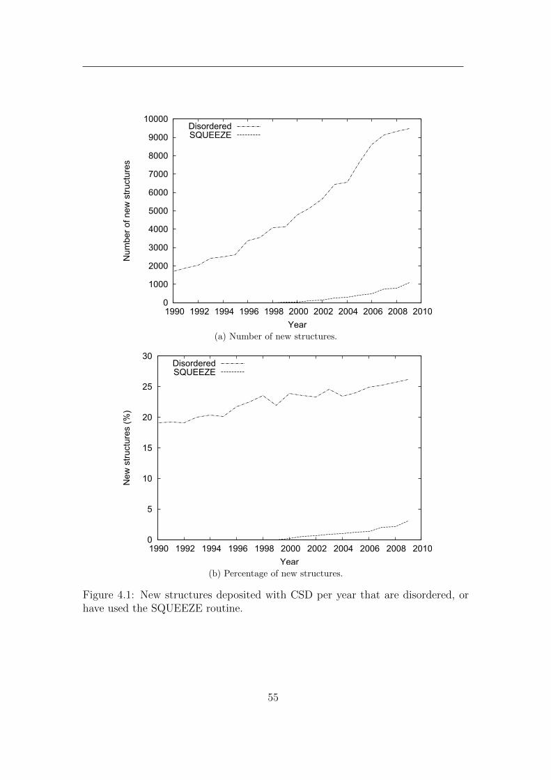
0

1000

2000

3000

4000

5000

6000

7000

8000

9000

10000

1990 1992 1994 1996 1998 2000 2002 2004 2006 2008 2010

Num

ber

of n

ew s

truc

ture

s

Year

DisorderedSQUEEZE

(a) Number of new structures.

0

5

10

15

20

25

30

1990 1992 1994 1996 1998 2000 2002 2004 2006 2008 2010

New

str

uctu

res

(%)

Year

DisorderedSQUEEZE

(b) Percentage of new structures.

Figure 4.1: New structures deposited with CSD per year that are disordered, orhave used the SQUEEZE routine.

55

every point in the unit cell to every structure factor:

ρ(x) = V −1∑h

|Fh| exp(iφh) exp(−2πih · x) (4.1)

F (h) =

∫cell

ρ(x) exp(2πih · x) dx. (4.2)

The crystallographic model is simply an interpretation of the measured electron

density, usually in terms of an atomic model. Therefore, any deficiencies in the

model can adversely affect the parameters of the ordered part of the model, as

their values change to compensate for deficiencies elsewhere in the least squares

minimisation. This can affect both the geometry of the molecule and also the

calculated standard uncertainties of refined and derived parameters. It is therefore

evident that it is important to account for any disorder in the best possible manner

during the process of crystal structure determination.

Orientational disorder is most commonly modelled with two or more overlap-

ping fragments, often requiring the extensive use of restraints and/or constraints

to keep the model chemically reasonable. When appropriate, a somewhat more

elegant alternative may be to model atoms as continuously disordered along some

special figure, such as a line, a ring or the surface of a sphere, as featured by the

program CRYSTALS [Schroder et al., 2004].

However, there are often cases where extensive disorder or unknown solvent

composition is such that neither approach is appropriate. Van der Sluis and Spek

[1990] suggested a method whereby the contribution to the calculated structure

factors of the disordered solvent area is calculated via a Fourier transform of that

area. This solvent contribution can then either be added to that calculated from

the ordered part of the structure, or alternatively subtracted from the observed

data before further cycles of refinement. This method has been made widely pop-

ular by the SQUEEZE routine available through the software PLATON [Spek,

2003]. As can be seen in Figure 4.1 it appears that this method is becoming in-

creasingly accepted as an appropriate method to deal with cases of severe disorder,

with, at the time of writing1, a total of over 4500 structures in the CSD where the

1CSD V5.32 database, November 2010 update

56

SQUEEZE routine has been applied, with over 1100 in 2009 alone.

4.2 Theory

The total calculated structure factor, F calch , can be considered as being composed

of two parts, that from the ordered atomic model of the structure, Fmodelh , and the

diffuse solvent1 contribution, F diffh . These are related according to

F calch = Fmodel

h + F diffh . (4.3)

The diffuse solvent contribution can be calculated from the discrete Fourier

transform of the electron density difference map over the solvent area

F diffh = Vg

∑xj∈S

∆ρ(xj) exp(2πih · xj), (4.4)

where Vg is the volume per grid point and S is the set of grid points xj that define

the solvent area.

This difference map is in turn calculated according to

∆ρ(x) = V −1∑h

[s∣∣F obs

h

∣∣ exp(iφcalch )

−∣∣Fmodel

h

∣∣ exp(iφmodelh )]

exp(−2πih · x),

(4.5)

where s is the overall scale factor,∣∣F obs

h

∣∣ is the observed structure factor, φmodelh is

the phase of Fmodelh , φcalch the phase of F calc

h and V is the volume of the unit cell.

We can optimize the diffuse scattering contribution, F diffh , by iteratively ap-

plying equations 4.5 and 4.4. Given the initial structure model, φcalch and the true

scale factor, s, are unknown. In the first cycle the true values are substituted with

φcalch = φmodelh and the scale factor obtained from the starting model is used. In

subsequent cycles, the phases and scale factor calculated using the provisional sol-

vent contribution from the previous cycle are used to provide an improved estimate

of the true values.

1The term “solvent” is used rather loosely throughout this chapter to include anions andcations, which could also be treated in the same way.

57

By examining equation 4.2 it is possible to see that when substituting h for

the 000 reflection, the resulting structure factor, F0 is equal to the integral of the

electron density over the whole unit cell, i.e. the total electron count of the unit

cell. The average density level of the difference map is zero and a summation of

the electron density over the solvent area gives the value

F0 =∑xj∈S

Vg∆ρ(xj), (4.6)

where the count over the region outside the solvent area is equal to −F0.

The average density of the difference map can be raised to such a level that

a summation over the points outside the solvent area gives zero, enabling an ap-

proximation of the number of electrons in the solvent region to be given by

F diff0 = F0[V/(V − Vs)], (4.7)

where Vs is the volume of the solvent region and V is the unit cell volume. A con-

tribution of F diff0 /V is added to ∆ρ(xj) before the next iteration of the procedure.

4.2.1 Refinement

Once the diffuse solvent contribution to the calculated structure factors has been

determined, it is then necessary to include this contribution in the refinement of the

ordered part of the structure. The most straightforward way of doing this would

be to refine against the total calculated structure factor as defined by equation 4.3.

This would be the preferred method if the desired refinement program is capable

of accepting fixed contributions to the structure factors, which is the case with our

own refinement program, smtbx-refine [Bourhis et al., 2011].

In order to use the method with the refinement program SHELXL [Sheldrick,

2008], an alternative approach is used to modify the observed structure factors:

F obs′

h = s∣∣F obs

h

∣∣ exp(iφmodelh )− F diffh (4.8)

58

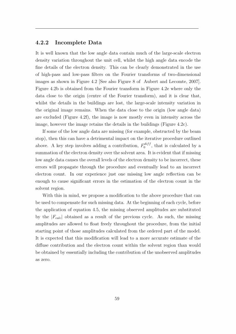
4.2.2 Incomplete Data

It is well known that the low angle data contain much of the large-scale electron

density variation throughout the unit cell, whilst the high angle data encode the

fine details of the electron density. This can be clearly demonstrated in the use

of high-pass and low-pass filters on the Fourier transforms of two-dimensional

images as shown in Figure 4.2 [See also Figure 8 of Aubert and Lecomte, 2007].

Figure 4.2b is obtained from the Fourier transform in Figure 4.2e where only the

data close to the origin (centre of the Fourier transform), and it is clear that,

whilst the details in the buildings are lost, the large-scale intensity variation in

the original image remains. When the data close to the origin (low angle data)

are excluded (Figure 4.2f), the image is now mostly even in intensity across the

image, however the image retains the details in the buildings (Figure 4.2c).

If some of the low angle data are missing (for example, obstructed by the beam

stop), then this can have a detrimental impact on the iterative procedure outlined

above. A key step involves adding a contribution, F diff0 , that is calculated by a

summation of the electron density over the solvent area. It is evident that if missing

low angle data causes the overall levels of the electron density to be incorrect, these

errors will propagate through the procedure and eventually lead to an incorrect

electron count. In our experience just one missing low angle reflection can be

enough to cause significant errors in the estimation of the electron count in the

solvent region.

With this in mind, we propose a modification to the above procedure that can

be used to compensate for such missing data. At the beginning of each cycle, before

the application of equation 4.5, the missing observed amplitudes are substituted

by the |Fcalc| obtained as a result of the previous cycle. As such, the missing

amplitudes are allowed to float freely throughout the procedure, from the initial

starting point of those amplitudes calculated from the ordered part of the model.

It is expected that this modification will lead to a more accurate estimate of the

diffuse contribution and the electron count within the solvent region than would

be obtained by essentially including the contribution of the unobserved amplitudes

as zero.

59

(a) (b) (c)

(d) (e) (f)

Figure 4.2: An image of the Chicago skyline (a) and its Fourier transform (d);(b) is the image reconstructed after application of a low-pass filter to the Fouriertransform (e); (c) is the image reconstructed after application of a high-pass filterto the Fourier transform (f). Fourier transforms calculated using the FTL-SEsoftware [JCrystalSoft, 2010].

60

4.2.3 Twinned Data

In order to obtain a correct electron density map in the case of twinned data, it is

necessary to first deconvolute, or ‘detwin’, the data. Detwinning of intensity data

and methods of doing so, are discussed in detail in §2.2. Regardless of the method

used to detwin the data, it is necessary to know the twin fraction(s) sufficiently

accurately in order to obtain a reasonable estimate of the untwinned intensities.

In our experience the twin fraction obtained through least squares refinement of

an incomplete model does not usually lead to a sufficiently accurate difference

electron density map for the solvent masking procedure to work well.

4.2.4 Standard Uncertainties

In the case of using a solvent mask as an alternative to modelling the solvent with

a disordered model and under the assumption that the model of the disorder is a

good fit to the data (at least comparable to that attained with the use of a solvent

mask), then it is to be expected that the standard uncertainties on the refined

parameters will be artificially reduced. The standard uncertainty for parameter pj

is given by

σ(pj) =

((A−1)jj

∑Ni=1wi∆

2i

N − P

)1/2

(4.9)

where A−1 is the inverse least squares normal matrix, wi∆2i are the weighted

residuals, for N observations and P parameters.

Under the assumption that the value of (A−1)jj is unchanged and that the fit

of the model to the data is identical in both cases, it is evident that the value of

the denominator will increase as the number of parameters decreases, thus causing

the standard uncertainty of the refined parameters to be underestimated.

Consider a hypothetical data set for which there are 4000 unique reflections

after merging with 316 parameters refined for the ordered part of the model. A

dichloromethane molecule is disordered over 3 orientations and each part is mod-

elled anisotropically for each atom (this is unlikely considering a 3 part disor-

der) and the positions of the hydrogen atoms are refined using riding constraints

[Watkin, 2008]. This gives a total of 27 parameters for each part (3 site param-

61

eters and 6 anisotropic displacement parameters per non-hydrogen atom). An

occupancy parameter is refined for each disorder component (with a restraint that

the sum of the occupancies is equal to unity), giving a total of 84 parameters to

model the disorder. From equation 4.9 a reduction in the standard uncertainties

of 1.15% would be expected after using the solvent masking procedure, taking into

account only the difference in the number of parameters. More realistically, only

the major disorder component is refined anisotropically, giving a total of 54 pa-

rameters required to model the disorder. Now a reduction of 0.74% in the standard

uncertainties would be expected. Since the number of data is usually much greater

than the number of parameters1, the reduction in the standard uncertainties due

to a change in the number of parameters is expected to be small.

It is important to remember, however, that the solvent masking procedure

is not intended as a replacement for correct atomic models of solvent disorder,

but rather as a complementary technique for the cases when an atomic model is

insufficient, or would lead to chemically nonsensical results. In such a case it is

expected that a significantly better fit of the model to the data can be obtained

using a solvent mask and hence the standard uncertainties would decrease by a

much greater amount than would be caused purely by the reduction in number of

refined parameters.

4.3 Method

The first step is to identify the areas of the unit cell that are accessible to solvent

molecules. A grid is set up where the grid step is chosen relative to the high

resolution limit, usually by a factor of 1/4. Initially all the grid points are set

to be 1. All points within a distance of ri from atom i, where ri is the sum of

the van der Waals radius and the solvent probe radius, rprobe, are set to 0. All

grid points with the value 0 are then tested to see if they are within a distance

rshrink of a grid point marked 1 and are themselves set to 1 if this is the case. The

grid points marked 1 are thus the solvent accessible region. This two-step process

1The current recommendation of the IUCr journals is for a data/parameter ratio > 10 for cen-trosymmetric and > 8 for non-centrosymmetric structures for a ‘quality structure determination’(http://journals.iucr.org/services/cif/checking/platon.html).

62

has the effect of smoothing the surface area of the solvent region relative to just

including all points that are outside the van der Waals radii of the atomic model.

The search for solvent accessible voids uses the procedure originally developed for

the cctbx bulk-solvent and scaling module [Afonine et al., 2005].

The above procedure acts in the space group P 1, however it can be optimised

by taking into account the space group symmetry. All atoms are moved to the

standardised asymmetric unit and this is expanded with symmetry equivalents

within a buffer region equivalent to the sum of the maximum van der Waals radius

and the solvent probe radius. Solvent accessible volumes are then carried out as

described previously and the space group symmetry is applied to the resulting map

to yield all the solvent regions in the unit cell. This approach gives substantial

speed increases for higher symmetry space groups and large unit cells.

Independent voids are then identified using a simple flood fill1 algorithm and,

for each void, a centre of mass and moment of inertia is calculated. Each void is

labelled with a sequential integer. The solvent accessible volume constitutes all

grid points with value greater than zero.

The solvent contribution to the structure factors is calculated following the

iterative procedure outlined in section 4.2.

4.4 Implementation

4.4.1 Computational Crystallography Toolbox

The procedure outlined above is implemented as part of the Small Molecule Tool-

box (smtbx) which is part of the Computational Crystallography Toolbox (cctbx)

[Grosse-Kunstleve et al., 2002].

The high-level code controlling the flow of the program is written in Python,

whilst the computationally intensive calculations (Fast Fourier Transform, void

search, structure factor calculations, etc.) are written using C++, which is exposed

to Python using the Boost.Python Library (http://www.boost.org/).

This combination allows for rapid prototyping of new ideas, whilst maintaining

the performance benefits of a compiled language.

1http://en.wikipedia.org/wiki/Flood fill

63

4.4.2 Olex2

The procedure is integrated within the Olex2 software package [Dolomanov et al.,

2009a], which can be used for visualisation of the calculated solvent accessible voids

and F diffh and F calc

h electron density maps. Once calculated, it is straightforward

to include the solvent mask in the refinement of the ordered part of the structure,

either with our own refinement program, smtbx-refine [Bourhis et al., 2011] or

alternatively with SHELXL [Sheldrick, 2008].

The details of the calculations and subsequent refinement are seamlessly prop-

agated into the CIF output by Olex2 ready for publication.

4.5 Test Structures

There are a number of tests that can be carried out to test the validity of the

procedure. In the first instance, a crystal structure can be taken where the solvent

content is both known and ordered. The procedure can be carried out using both

the original observed data and using structure factors calculated from the model,

and with and without prior least squares refinement. The electron count estimated

by the procedure should be close to that expected for the solvent that is omitted

from the model and the subsequent least squares procedure should give a similar

outcome to that obtained with an atomic model of the solvent.

The completion of missing data can be tested similarly using a test case with

ordered solvent, where one or more low angle reflections are missing (or manually

omitted) and the results of the procedure can be compared with and without

using the set completion technique. The amplitudes of the omitted reflections can

be followed throughout the iterations, in order to observe whether their values

converge close to the true values.

The outcomes of the procedure obtained for several test structures and appli-

cations are tabulated in Table 4.1. Analysis of the differences in geometry after

the procedure is presented in Table 4.2.

64

Compound I

1-methyl-3-phenyl-7,8-dimethoxy-3H-pyrazolo(3,4-c)isoquinoline acetonitrile sol-

vate [Bogza et al., 2005, CSD code YAKRUY], space group P 1, a = 7.086(1),

b = 10.791(3), c = 12.850(2) A, α = 104.16(2)◦, β = 105.87(2)◦, γ = 95.86(1)◦,

containing one acetonitrile molecule per asymmetric unit.

A synthetic data set was created from the full atomic model to dmin = 0.7 A

with 100% completeness. The acetonitrile solvate molecule was then discarded

from the model with the solvent masking procedure used in place. An electron

count of 43.4 was found for a single void per unit cell, with volume 174 A3. The

structure refined to R1 = 0.88% using unit weights. The 001 reflection was then

discarded and the procedure repeated, with the resulting electron count of 40.5 and

R1 = 1.81%. The procedure was run once more, this time using the set completion

technique, giving an electron count of 43.4 and R1 = 0.89%.

To test the technique more extensively, approximately 5% of the reflections were

discarded at random, resulting in a completeness of 95.3% (Figure 4.3). Without

the use of the set completion technique, an electron count of 34.5 was obtained

and R1 = 5.20%. Using the set completion technique gave an electron count of

43.4 and R1 = 0.89%. The amplitudes of three of the omitted low angle reflections

were followed at each iteration. From the results shown in Figure 4.4 it can be

seen that in each case the amplitude of the reflection converges close to the ‘true’

value.

Compound II

1(2,5)-Thiophena-3,7-dioxa-2,8-dioxo-5(5,5’)(9,10-bis(4-methyl-1,3-dithiol-2-

ylidene)-9,10-dihydroanthracena)cyclo-octaphane dichloromethane solvate

[Godbert et al., 2001, CSD code QIPZEU], space group P21/c, a = 11.407(5),

b = 17.160(8), c = 15.607(7) A, β = 99.83(2)◦. The asymmetric unit contains one

dichloromethane molecule which is disordered over two orientations, modelled

with 50% occupancy for each position. The refinement converges to R1 = 7.15%

for 2901 reflections where I ≥ 2u(I). Bond similarity restraints on the C-Cl

distances were required in order to keep the geometry of the dichloromethane

molecule chemically reasonable. Alternatively a solvent mask was used instead

65

0

20

40

60

80

100

0 10 20 30 40 50 60 70

She

ll co

mpl

eten

ess

Resolution (2θ)

Figure 4.3: The completeness in resolution shells for compound I after approxi-mately 5% of the reflections were discarded at random.

0

5

10

15

20

25

30

35

40

0 1 2 3 4 5 6 7

|Fo|

Iteration

(-1 0 1)( 0 -2 2)( 1 -2 1)

Figure 4.4: The amplitudes of three ‘floating’ missing structure factors at eachiteration of the solvent masking procedure. The lightly dashed horizontal linesindicate the ‘true’ amplitudes.

66

of modelling the dichloromethane atomically. Two symmetry-related voids were

found in the unit cell, each with a volume of 235 A3

and an estimated electron

count of 79.7 per void. Refinement using the solvent mask gave a slightly reduced

R1 = 6.99%. Although the completeness was high (99.98%) to 2θ = 50◦, it was

noted that the (100) reflection was not measured. The solvent masking procedure

was repeated using the set completion technique, giving an estimated electron

count of 84.8 and a marginally lower R1 = 6.95% after refinement to convergence.

Although there was not a significant change in the R1-factor, the estimated

electron count obtained using the set completion technique was much closer to

the expected value for two dichloromethane molecules (2× 42e− = 84e−).

Compound III

9-(4-chlorophenyl)-5,6-dimethoxy-10,11,19-triazatetracyclo[9.8.0.03,8.013,18]

nonadeca-1(19),3(8),4,6,13(18),14,16-heptaen-12-one acetone solvate [Bat-

sanov, 2000], space group C2/c, a = 20.085(5), b = 7.717(1), c = 28.907(3) A,

β = 97.77(1)◦. The asymmetric unit contains half an acetone solvate molecule

sited on a special position. Refinement of the full atomic model converges to

R1 = 5.03%. The acetone molecule was then discarded in the model and the

solvent masking procedure was used in its place. Four voids were found per unit

cell, each with a volume of 124 A3

and an estimated electron count of 25.9 and

R1 = 5.11%. It was noted that the (002) reflection was missing and therefore the

procedure was repeated using the set completion technique, giving an electron

count of 32.9 and R1 = 5.00%.

Compound IV

Tetrachloro-(1,2-bis(diphenylphosphoryl)ethane-O,O’)-tin(iv) acetone solvate

[Batsanov et al., 2009, CSD code QOZQAY], space group P 1, a = 9.796(2),

b = 11.497(1), c = 16.171(3) A, α = 99.91(1)◦, β = 102.85(1)◦, γ = 110.81(1)◦.

The structure contains one acetone molecule per asymmetric unit, which is

disordered over two parts in the ratio 80:20. With the use of bond similarity

restraints, the refinement converges to R1 = 2.64% for 7533 reflections where

I ≥ 2u(I). When a solvent mask was used instead of the atomic model of

67

the disordered acetone, one void was found in the unit cell with a volume of

309 A3

with an estimated electron count of 63.6 electrons per unit cell. This is

comparable to the expected count for two acetone molecules (2 × 32e− = 64e−).

Refinement using the solvent mask converged to R1 = 2.47%.

4.6 Applications

Compound V

1,13(1,4)-Dibenzena-7,19(2,6)-bis(9,10-bis(4,5-bis(methylthio)-1,3-dithiol-2-

ylidene)-9,10-dihydroanthracena)-3,6,8,11,15,18,20,23-octaoxa-2,12,14,24-

tetraoxotetracosaphane dichloromethane hexane solvate [Christensen et al.,

2001, CSD code QOSDIL], space group P 1, a = 14.525(2), b = 15.647(2),

c = 18.238(2) A, α = 88.59(2)◦, β = 86.97(2)◦, γ = 79.82(2)◦. The

dichloromethane and hexane molecules are severely disordered along chan-

nels through the unit cell. In the original publication the disorder was modelled

with arbitrary chlorine and carbon atoms, with R1 = 7.63%. Five of the six

largest residual electron density peaks (0.6 − 0.65 e− A−3

) are found within the

solvent region. After application of the solvent masking procedure, R1 = 6.73%

and the highest residual electron density peak (0.64 e− A−3

) is close to one of

the sulphur atoms, with no significant residual electron density peaks within the

solvent region. A single void was found that runs along a channel parallel to the

b-axis, with volume 596 A3

and an estimated electron count of 143.5 electrons per

unit cell.

Compound VI

2-(3’-(t-Butyldimethylsiloxy)-1’-oxo-1’,3’-dihydroisoindol-3’-yl)-1,2’-propano-1,2-

dicarba-closo-dodecaborane pentane solvate [Batsanov et al., 2001, CSD code

QOYXOR], space group P 1, a = 14.448(1), b = 14.680(1), c = 16.137(1) A,

α = 101.58(1)◦, β = 90.07(1)◦, γ = 96.13(1)◦. The pentane solvent is severely

disordered along channels through the unit cell. In the published structure the

disordered solvent is modelled with arbitrary carbon atoms of varying fixed

68

occupancy, with R1 = 8.35%. The ten largest residual electron density peaks

(0.65− 0.79 e− A−3

) are found within the solvent region. After application of the

solvent masking procedure (electron count = 117.7), R1 = 6.15% and there are

no significant residual electron density peaks within the solvent region. However,

it was noted that there were several missing low angle reflections, (001), (100),

(010), (−101) and (101). The procedure was repeated using the set completion

technique, resulting in a significantly larger electron count of 235 and R1 = 5.57%.

Compound VII

Space group R3, a = 27.065(3), b = 27.065(3), c = 24.318(3) A [Batsanov,

2009]. Hexane solvent molecules are severely disordered along the 3-fold axis.

After refinement with no attempt made to model the solvent, an R1-factor of

9.24% was achieved. The 15 largest residual electron density peaks (in the range

0.5 − 1.3 e− A−3

) are all in the channel parallel to the c-axis (Figure 4.5a). The

solvent masking procedure found 3 symmetry equivalent voids parallel to the c-

axis, giving a total solvent accessible volume of 3687 A3

per unit cell (24% of the

unit cell volume) and an estimated electron count of 866 electrons per unit cell.

Figure 4.6 shows the electron density map for F diff as displayed in Olex2. A

much improved R1-factor of 4.60% was obtained for 2564 reflections I ≥ 2u(I).

No significant residual electron density was observed in the voids and the highest

residual electron density peaks (< 0.4 e− A−3

) were in the vicinity of the atomic

model (Figure 4.5b).

4.7 Discussion

It is encouraging that for Compound I the set completion technique gives much

improved results for the cases where there are missing reflections. Almost identical

results are obtained compared to the complete data set, even for the case where

almost 5% of the reflections are missing. Compounds II and III demonstrate that

the set completion technique gives estimated electron counts closer to the expected

value when used with original data sets where one or more low angle reflections are

unobserved. From Table 4.2 it can be seen that only relatively small decreases in

69

(a) The 15 highest residual electron density peaks are all found within thechannel parallel to the c-axis.

(b) After the use of a solvent mask there are no significant residual electrondensity peaks within the solvent channels.

Figure 4.5: The view of the unit cell down the c-axis for compound VII. The peaksin the difference electron density are displayed as transparent light-brown spheres.

70

(a) The view down the c-axis.

(b) The view perpendicular to the ab vector.

Figure 4.6: Two alternate views of electron density map for F diff for compoundVII.

71

Atomic model Mask Set completion

Compound Solvent R1(%) e− R1(%) e− R1(%) e− Vs(A)3

Vs(%)I CH3CN 0.00 44 0.88 43.4 - - 186 20.6

I† CH3CN 0.00 44 1.81 40.5 0.89 43.4 186 20.6

I‡ CH3CN 0.00 44 5.20 34.5 0.89 43.4 186 20.6II CH2Cl2 7.15 84 6.99 79.7 6.95 84.8 479 15.6III (CH3)2CO 5.04 128 5.11 103.6 5.00 131.6 497 11.2IV (CH3)2CO 2.64 64 2.47 63.6 - - 309 19.4V CH2Cl2, C6H14 7.63 - 6.73 143.5 - - 596 14.6VI C5H12 8.35 - 6.15 117.7 5.57 235 1103 33.1VII C6H14 9.24 - 4.60 865.8 - - 3844 24.9

Table 4.1: Comparisons of the results obtained using the solvent masking pro-cedure with and without the set completion technique and the original atomicmodels. Vs is the total solvent accessible volume per unit cell. Also given isthe solvent accessible volume as a percentage of the unit cell volume. †The 001reflection was rejected. ‡Approximately 5% of the reflections were discarded.

Bond lengths (A) Bond Angles (◦)Compound RMS deltas s.u. % decrease RMS deltas s.u. % decreaseII 0.00328 5.7 0.24015 5.5III 0.00099 1.7 0.07437 1.9IV 0.00068 6.7 0.03596 7.1V 0.00507 18.1 0.27379 17.0VI 0.00416 37.5 0.14702 37.0VII 0.01527 56.8 0.78640 54.4

Table 4.2: The root mean square (RMS) differences in bond lengths and angles,and the percentage decrease in their standard uncertainties after application of thesolvent masking procedure.

72

the standard uncertainties of the geometrical parameters are observed compared

to those obtained when using an atomic model. Whilst for these test compounds

a full atomic model of the solvent is undoubtedly the correct approach to take, the

results show that the solvent masking procedure can give comparable results.

All three applications show significant improvements after the use of the pro-

cedure and larger decreases in the standard uncertainties are observed, ranging

from 17% for Compound V to > 50% for Compound VII. After the use of the set

completion technique to compensate for several missing low angle reflections, the

estimated electron count obtained for Compound VI is significantly larger with an

improved least squares fit. This difference in electron count could be significant

when attempting to estimate the solvent composition of the crystal. Compounds

V and VI were both published before the method of van der Sluis and Spek [1990]

was popularised (Figure 4.1) and consequently arbitrary atoms of varying types

and occupancies were used to model the severely disordered solvents. Given that

the current procedure gives demonstrable improvements in both the least squares

fit and the geometry of the ordered part of the structure whilst also giving further

information in terms of the estimated electron count which may be useful in identi-

fying the solvent composition (in conjunction with ancillary information), it is the

author’s opinion that it is more meaningful to use the solvent masking procedure

in such cases, provided the use and outcomes of the procedure are clearly reported.

73

Chapter 5

The Crystallographic Information

Framework (CIF)

5.1 iotbx.cif

5.1.1 Introduction

The CIF (Crystallographic Information File) syntax [Hall et al., 1991] has become

firmly established [Brown and McMahon, 2002] as the file format for deposition

and archiving of small molecule crystal structures, and increasingly their structure

factors. Whilst the PDB is still the preferred file format for deposition of macro-

molecular crystal structures, the CIF format is nonetheless important to macro-

molecular software through their extensive use of the PDB chemical components1

and REFMAC monomer libraries [Vagin et al., 2004]. The IUCr maintain CIF dic-

tionaries for describing the results of powder diffraction [Toby, 1998] and electron

density studies [Mallinson, 2003], and for describing incommensurately modulated

crystal structures [Madariaga, 2002]. The Crystallography Binary Format (CBF)

and Image-supporting Crystallographic Information File (ImgCIF) [Hammersley

et al., 2003] are extensions to the CIF format to support inclusion of binary data

in the CIF, in particular raw experimental data from area detectors. The CIF is

probably one of the most well known file formats within the field of chemistry,

1http://www.wwpdb.org/ccd.html

74

since it is predominantly the form in which synthetic chemists receive the results

of a crystal structure analysis carried out on their behalf.

Evidently the CIF is intrinsically involved in a wide variety of crystallographic

applications from data collection to publication and archiving of the outcomes of

crystallographic studies. In addition there is a wealth of crystal structure coordi-

nates and reflection data freely available in the CIF format through the Crystal-

lographic Open Database (COD) [Grazulis et al., 2009] and the large quantity of

data available as supplementary material for papers published in IUCr journals,

for which many possible uses can be imagined. As such it is vital for a crystallo-

graphic library such as the cctbx to provide high quality tools for reading, creation

and manipulation of CIFs, and extraction of crystallographic data from them.

Several CIF programming libraries have been developed for various languages,

including FORTRAN [Hall and Bernstein, 1996], C [Ellis and Bernstein, 2001;

Westbrook et al., 1997], Objective C [Chang and Bourne, 1998], .NET [Lin, 2010],

Perl [Bluhm, 2000] and Python [Hester, 2006]. For some time PyCIFRW [Hester,

2006] has been distributed with the cctbx source code bundles, however there was

only limited support within the cctbx for PyCIFRW. Since the parsing of CIF

files in PyCIFRW occurs using an interpreted language (Python [Python Software

Foundation]), parsing of extremely large CIFs (e.g. reflection files, dictionary files)

can be considerably slower than when using comparable compiled parsers. As a

result there existed several partial CIF parsers within the cctbx, each hand-crafted

to suit the specific task in hand (separate tools for reading the PDB chemical

components and REFMAC monomer libraries; as part of the phenix.cif as mtz

tool; for reading fcf reflection files as output by SHELXL [Sheldrick, 2008]).

During the development of the tools described in earlier chapters within the

context of the smtbx and Olex2, it became apparent that the CIF format would

play a central part in presenting the results of the procedures developed, in addition

to a need for providing an interface for managing the contents of the CIF within

Olex2. Therefore it was decided to implement a new CIF framework within the

iotbx (input/output toolbox) module of the cctbx.

Given the availability of a clearly defined formal grammar for the CIF syntax1,

it was decided to use the ANTLR parser generator [Parr, 2007] for generation of a

1http://www.iucr.org/resources/cif/spec/version1.1/cifsyntax

75

lexer and parser from a formally defined grammar. ANTLR was chosen because of

its support for multiple programming languages, in particular its support of Python

and C/C++. In addition, the associated ANTLRWorks GUI development envi-

ronment features a number of tools that aid the development of grammars, such

as visualisation of syntax diagrams and rule dependency graphs. This enabled the

majority of the development to be focused on the design of the internal represen-

tation of the CIF model, whilst ensuring that the resulting parser closely follows

the formal CIF grammar. The code is structured in such a way that the parser is

quite distinct from the model, meaning an alternative representation of the model

could be used with the same parser, and conversely a different parser could be used

to populate the existing iotbx.cif model. The CIF grammar in ANTLR format is

included in Appendix B. This grammar is suitable for generating CIF parsers in

any of the programming languages supported by ANTLR (including C, C#, Ob-

jective C, Java, JavaScript, Python, Ruby). Figure 5.1 shows a simplified rule

dependency graph generated for the CIF grammar using the ANTLRWorks GUI.

5.1.2 Using iotbx.cif

Developers familiar with the built-in dictionary type of the Python programming

language [Python Software Foundation] will be immediately at home with the

syntax of the iotbx.cif representation of the CIF model.

The top level object is iotbx.cif.model.cif, which is the type equivalent to a

full CIF file. This contains zero or more data blocks, which are accessed by data

block name using the traditional Python dictionary square brackets notation for

accessing a dictionary by key. Using a valid data block name, this returns a

CIF data block of the type iotbx.cif.model.block. A CIF data block consists of a

sequence of data items and associated values. A data item can be associated with

either one value, or a list of values (as part of a CIF loop), and a given data item

can only be found once per data block. These values can in turn be accessed using

the square bracket notation to retrieve the value(s) associated with a specified data

item (tag).

76

Figure 5.1: A simplified rule dependency graph for the CIF grammar.

77

import i o tbx . c i f

c i f m o d e l = iotbx . c i f . r eader ( f i l e p a t h=’ myf i l e . c i f ’ ) . model ( )

c i f b l o c k = c i f m o d e l [ ’ my block name ’ ]

ha l l symbo l = c i f b l o c k [ ’ space group name Hal l ’ ]

Then:

>>>print ha l l symbo l

−P 2yn

Looped items are stored by columns, and the full list for a given looped item

can be accessed by the data name as shown below.

>>>sym ops = c i f b l o c k [ ’ space group symop operat ion xyz ’ ]

>>>for sym op in sym ops :

. . . print sym op

x , y , z

−x+1/2 ,y+1/2,−z+1/2

−x,−y,−z

x−1/2,−y−1/2 ,z−1/2

The full loop object can be extracted by the name of the loop. The name of

the loop is taken to be the longest common substring starting with an underscore

character, and followed by (but not including) an underscore (in the case of DDL1

CIFs) or point (in the case of DDL2 CIFs) character separator. This follows the

IUCr guidelines for reserved prefixes for local dictionary extensions1. Once a loop

has been extracted, this can then be used to iterate through by rows, or to add

further rows or columns to the loop. The following example demonstrates the

creation of a CIF loop describing the given distance restraints.

loop = model . loop ( header=(

” r e s t r d i s t a n c e a t o m s i t e l a b e l 1 ” ,

” r e s t r d i s t a n c e a t o m s i t e l a b e l 2 ” ,

” r e s t r d i s t a n c e s i t e s y m m e t r y 2 ” ,

” r e s t r d i s t a n c e t a r g e t ” ,

” r e s t r d i s t a n c e t a r g e t w e i g h t p a r a m ” ,

” r e s t r d i s t a n c e d i f f ” ) )

for proxy in pr o x i e s :

r e s t r a i n t = g e o m e t r y r e s t r a i n t s . bond (

u n i t c e l l=u n i t c e l l ,

1http://www.iucr.org/resources/cif/spec/ancillary/reserved-prefixes

78

s i t e s c a r t=s i t e s c a r t ,

proxy=proxy )

loop . add row ( (

s i t e l a b e l s [ proxy . i s e q s [ 0 ] ] ,

s i t e l a b e l s [ proxy . i s e q s [ 1 ] ] ,

s p a c e g r o u p i n f o . c i f symmetry code ( proxy . r t m x j i ) ,

r e s t r a i n t . d i s t a n c e i d e a l ,

math . s q r t (1/ r e s t r a i n t . weight ) ,

r e s t r a i n t . d e l t a ) )

c i f b l o c k . add loop ( loop )

5.1.2.1 CIF output

CIF objects (model.cif, model.block, model.loop) can be exported in several ways.

The simplest way is using the Python ”print” statement as follows:

f = open ( ’ my f i l e . c i f ’ , ’w ’ )

print >> f , my ci f model

f . c l o s e ( )

The show() method of the CIF objects allows more fine-tuning of the output,

including the amount of indentation used for looped data and the width of the

data name field. For more advanced formatting, a Python formatting string can

be provided to control the output of individual loops (in contrast to the default

behaviour where items are single space-separated). The following example demon-

strates the use of the tools provided by iotbx.cif to output reflection data in a

format similar to that output by SHELXL using the ‘LIST 4’ instruction:

f = open ( ’ my f i l e . f c f ’ ) , ’w ’ )

c i f = iotbx . c i f . model . c i f ( )

m a s a s c i f b l o c k = iotbx . c i f . m i l l e r a r r a y s a s c i f b l o c k (

f c a l c s q , a r ray type=’ c a l c ’ )

m a s a s c i f b l o c k . a d d m i l l e r a r r a y ( f o b s s q , a r ray type=’ meas ’ )

c i f [ ’ my block name ’ ] = m a s a s c i f b l o c k . c i f b l o c k

f o r m a t s t r i n g=’%−4i ’ ∗3 + ’%−12.2 f ’ ∗2 + ’%−10.2 f ’

c i f . show ( out=f , l o o p f o r m a t s t r i n g s={ ’ r e f l n ’ : f o r m a t s t r i n g })

f . c l o s e ( )

Below is an example of part of the refln * loop generated by this short script.

79

l o op

r e f l n i n d e x h

r e f l n i n d e x k

r e f l n i n d e x l

r e f l n F s q u a r e d c a l c

r e f l n F squa r ed meas

r e f l n F s q u a r e d s i g m a

0 0 1 129 .73 59 .30 3 .63

0 1 0 157 .87 157 .99 4 .45

0 1 1 176 .00 185 .32 3 .75

1 0 0 142 .63 141 .28 2 .62

0 −1 1 2024.44 2010.97 30 .75

5.1.3 Validation of CIFs against data dictionaries

Successful parsing without errors of a given CIF indicates only that it is syntac-

tically correct. CIF dictionaries allow for a machine-readable formal description

of allowed data items, and for possible restrictions on the attributes of their as-

sociated values. A collection of application-specific dictionaries are maintained by

the Committee for the Maintenance of the CIF Standard (COMCIFS), and can

be used to validate the contents of a given CIF. The CIF data dictionaries abide

by the CIF syntax, with two distinct dictionary definition languages (DDL1 and

DDL2) currently in use.

In the context of iotbx.cif, once loaded, a CIF can be validated as follows:

from i o tbx . c i f import v a l i d a t a t i o n

c i f d i c = v a l i d a t i o n . s m a r t l o a d d i c t i o n a r y (name=’ c i f c o r e . d i c ’ )

c i f m o d e l . v a l i d a t e ( c i f d i c , show warnings=True )

The smart load dictionary function allows for a dictionary to be loaded from a

variety of sources, including a locally stored version, downloaded from an arbitrary

URL, or via lookup in a cif dictionary register1 allowing use of the most up-to-date

version of the dictionary. A list of potential errors and warnings found during the

validation is output by the procedure. The error handling is designed such that it

1e.g. ftp://ftp.iucr.org/pub/cifdics/cifdic.register

80

is possible for an application making use of iotbx.cif to override the default error

handler with one specific to the needs of the application.

5.1.4 Interconversion with cctbx crystallographic objects

An essential part of any crystallographic library or software is a means to easily

export/extract crystallographic information to/from the CIF format. As such, two

key crystallographic objects in the cctbx, namely xray.structure and miller.array,

have methods enabling easy interconversion of either object with a CIF.

from cctbx import mi l l e r , xray

x r a y s t r u c t u r e = xray . s t r u c t u r e . f r o m c i f ( f i l e p a t h=’my. c i f ’ )

x r a y s t r u c t u r e . show summary ( )

m i l l e r a r r a y s = m i l l e r . array . f r o m c i f ( f i l e p a t h=’my. f c f ’ )

f c a l c s q = m i l l e r a r r a y s [ ’ r e f l n F s q u a r e d c a l c ’ ]

f o b s s q = m i l l e r a r r a y s [ ’ r e f l n F squa r ed meas ’ ]

f o b s s q . show comprehensive summary ( )

Tools have been developed in order to support output of the requisite struc-

tural information for publication of a structure determination. This includes the

export of an xray.structure into CIF format, and also the inclusion of geometrical

features such as bonds and angles. Optionally the covariance matrices for the re-

fined parameters and for the unit cell parameters can be provided to enable the

calculation of standard uncertainties for both refined and derived parameters (see

also §2.3).

Support was recently added for the new restraints CIF dictionary [Brown and

Guzei, 2011] which is intended to allow for the description in CIF format of the

restraints and constraints used in a least-squares refinement.

5.1.5 Performance

Since the program uses a compiled parser rather than a pure Python parser, it is

expected that parsing would be of sufficient speed to make handling of large CIF

files acceptable, particularly for the case of reading in files containing structure

factors. To test the performance of the parser and the procedures extracting

81

File ext. No. files Build errors Parsing errors CPU time (s) Average (ms)cif 136405 - 3 2409 18cif 136405 1943 3 3549 26hkl 13738 - 21 1845 134hkl 13738 83 21 2121 154

Table 5.1: Performance of iotbx.cif when tested on the Crystallography OpenDatabase (COD) using a server with 4 times AMD 12-core OpteronTMProcessor6174, 2.2GHz, running Fedora 14.

File name File size Read time (ms) Write time (ms) Validation time (ms)(kB) (a) (b) (a) (b) (a) (b)

fg3210.cif 25 26 34 20 25 41 47fg3210CPsup2.hkl 84 43 51 117 150 48 584hhb.cif 705 733 891 1830 2309 2023 1955cif core 2.4.1.dic 469 125 191 78 102 254 298mmcif std 2.0.09.dic 1717 729 1057 356 461 1549 2018

Table 5.2: Execution times on (a) Intel R©CoreTM2 Duo E6750 PC, 2.66 GHz,3GB RAM running Windows Vista, and (b) Server with 4 times AMD 12-coreOpteronTMProcessor 6174, 2.2GHz, running Fedora 14.

crystallographic information, a short script was run over all the CIF files in the

Crystallography Open Database (COD) [Grazulis et al., 2009].

A total of 136405 CIF files were parsed in 2409 seconds of CPU time, at an

average of 18 ms per file. 3 files were found to contain syntax errors; the remain-

ing all parsed successfully. The procedure was repeated constructing instances of

xray.structure; a total of 134462 instances were successfully constructed in 3549

seconds of CPU time, at an average of 26 ms per file. Table 5.1 also gives the results

obtained when the procedure was run over 13738 CIF format reflection files found

in the COD. The average parsing time for a reflection file was 134 ms, increasing to

154 ms when construction of a miller.array was attempted after parsing. Table 5.2

gives the performance of iotbx.cif tools on typical small molecule and protein data

files and two selected dictionary files.1

The results show good performance for both the parser and the procedures

extracting crystallographic information from the CIF model. With the increasing

availability of multi-core processors, it is clear that, in conjunction with the large

14hbb.cif was downloaded from the PDB website [Fermi et al., 1984]; fg3210.cif andfg3210CPsup2.hkl were obtained from the IUCr website [Yufit and Howard, 2011].

82

number of tools provided by the cctbx, the iotbx.cif is suitable for performing

large-scale analyses of crystal structures, since the overhead of reading structures

from CIFs is minimal.

The performance of CIF output for files containing loops with a large number of

values can be improved significantly by using the advanced loop formatting option

described in §5.1.2.1, since each value will no longer be checked individually to

determine if quoting of the value is necessary.

5.1.6 Common CIF syntax errors and error recovery

As a result of comprehensive testing of the iotbx.cif parser a number of commonly

encountered syntax errors were identified, some of which are listed below. Among

the sources of CIF files used are the Crystallography Open Database (COD), a

selection of CIFs obtained from the websites of IUCr journals, the PDB chemical

components library, the REFMAC monomer library and an in-house database of

crystal structures.

1. Missing starting or closing quotes.

2. Missing starting and closing quotes for a string containing whitespace.

3. Some text prepended to CIF but not using CIF comment format (e.g. Check-

CIF output).

4. Mismatching semicolons.

5. More than one data value per tag.

6. Missing data value for a tag.

7. Incomplete CIF - e.g. missing data block heading

8. Intended data block heading contains whitespace or illegal character(s). This

can happen if a program uses the file name as the data block heading when

creating a CIF but does not remove/substitute whitespace or illegal charac-

ters.

83

9. Non-ASCII characters - data values have been “copy and pasted” from other

sources, for example, this could be an author’s name or place name.

10. Unquoted string with ’[’ as the first character.

11. Wrong number of values for loop.

Item 10 was the syntax error most commonly observed in the publicly available

databases (i.e. excluding the in-house database). The CIF grammar explicitly

forbids the characters ‘[’ and ‘]’ from being the first character of an unquoted

string1:

Matching square bracket characters, ’[’ and ’]’, are reserved for possi-

ble future introduction as delimiters of multi-line data values. At this

revision of the CIF specification a data value may not begin with an

unquoted left square bracket character ’[’. (While not strictly neces-

sary, the right square bracket character ’]’ is restricted in the same way

in recognition of its reserved use as a closing delimiter.)

It appears that the syntax checking routines used by the IUCr and the COD,

and also CheckCIF/PLATON do not currently consider this a syntax error, which

is in conflict with the formal definition of the CIF grammar.

The most commonly encountered syntax error for CIF format reflection files is

item 11, although this error can affect any CIF containing a loop. The number

of values in a loop must be an exact multiple of the number of tags in the loop

header and it is an error if this is not the case. This is probably the hardest error to

diagnose since it is not associated with a specific line number, only the particular

loop, which may be many thousands of lines long in the case of reflection data, and

hence the entire loop is rendered invalid. Frequently this error can be attributed to

manual editing of the file resulting in one or more value being accidentally deleted.

More worryingly, it is occasionally the result of a program outputting the data in

fixed-field format when one of the values takes up the full width of its fixed field,

losing a whitespace separator in the process. One such example can be found on

line 3708 of the file sk1436Isup2.hkl which can be obtained from the supplementary

materials accompanying Picard et al. [2001]:

1http://www.iucr.org/resources/cif/spec/version1.1/cifsyntax#general

84

line 3708: 0 0 42 40917268.00 43615084.002105532.75 o

This highlights one of the dangers of attempting to combine fixed-width formatting

with a whitespace separated file format such as the CIF.

Some of the syntax errors outlined above are to varying extents recoverable

parsing or lexing errors. Missing quotes potentially can be detected and miss-

ing tokens inserted when an end-of-line (EOL) character is encountered, since a

quoted string can not extend past an EOL character. For errors such as multiple

values for a tag that is not part of a loop, or a tag with no value given, the parser

may recommence parsing at the next valid token it finds, discarding those invalid

tokens. For invalid characters (items 9 and 10) the invalid characters can either

be accepted, or the offending tag-value pair can be discarded (the current imple-

mentation does the latter). The most dangerous error is that of a missing closing

semicolon for a semicolon text field, since the rest of the file up until the end-of-file

(EOF) character is consumed as part of the semicolon text field. Upon reaching

the EOF character an error is emitted by the lexer, but recovery from this error

is not possible.

On the one hand, it may be desirable for a program to be as accommodating

of errors as possible on input whilst ensuring that the output is as correct as

possible. On the other hand, there are clear advantages in having software that

raises clear errors when syntax errors are encountered, as this would discourage the

proliferation of incorrectly formed CIFs. Indeed, one would not expect a computer

code compiler to be accepting of errors, syntax or otherwise, in source code files.

The syntax errors observed generally fall into two categories: either as the re-

sult of manual editing of the CIF introducing some error; or some bug or oversight

on behalf of the crystallographic software used to create or manipulate the CIF in-

troduces a syntax error. The latter category of error can be fixed easily if software

authors are aware of any potential pitfalls in CIF output. It should be the aim of

every crystallographic program that creates CIFs to ensure that they are syntac-

tically correct. Errors that are introduced by manual editing can be eliminated if

there exists software that provides the means to manage the information output in

the CIF with minimal effort. The following section describes the steps that have

been made to address both of these issues within Olex2. If further editing of the

85

CIF is required, it would be preferable to use a dedicated tool such as enCIFer

[Allen et al., 2004] or publCIF [Westrip, 2010] instead of manual editing of the file

since these provide comprehensive syntax and dictionary validation in addition to

many other tools to aid preparation of the final CIF.

5.1.7 Discussion

With the addition of the iotbx.cif module, the cctbx module now comprehensively

supports most major small molecule and macromolecular crystallographic file for-

mats (SHELX ins/res and hkl, CIF, PDB1, CCP4 maps2, X-PLOR format3, MTZ

format4 and others).

The iotbx.cif module is now used heavily in the Olex2 software, as described

in the following section. Additionally, the tools provided by the iotbx.cif module

are currently being used extensively, in conjunction with the COD as a source

of structural models and associated reflection data, in the evaluation of different

approaches to minimization, including full-matrix, conjugate gradient, lbfgs and

new algorithms under development [Grosse-Kunstleve, 2011].

5.2 CIF as a publication and archiving format

Publication of a small molecule crystal structure usually requires the submission

of the results of the structural determination in a CIF format file, with increas-

ingly the structure factors also required in CIF format. In addition, publication

within an IUCr journal usually requires the use of the IUCr full validation suite

(checkCIF/PLATON 5), which performs a large number of consistency checks to

highlight any potential errors in the structure determination or reporting of the

results [Spek, 2009].

A published CIF will contain information from numerous sources at various

stages of the crystal structure determination process: data collection, data pro-

1http://www.wwpdb.org/documentation/format32/v3.2.html2http://www.ccp4.ac.uk/html/maplib.html3http://psb11.snv.jussieu.fr/doc-logiciels/msi/xplor981/formats.html4http://www.ccp4.ac.uk/html/mtzformat.html5http://journals.iucr.org/services/cif/checking/checkfull.html

86

cessing, structure solution, structure refinement and molecular graphics software,

to name but a few. Tools for aggregating information related to the structure at

hand were developed within the Olex2 software and are available as part of the

Report module. Relevant information is automatically extracted from experimen-

tal files present in the working directory (e.g. numerous Bruker-specific output

files, Agilent *.cif od, Rigaku CrystalClear.cif). Further information can be en-

tered through the GUI where there are sections containing fields relevant to the

diffraction, crystal and publication sections of the CIF. Details entered during

the report stage about authors, journals and diffractometers are stored locally, to

avoid having to input the same data repeatedly for different structures (as most

people tend to collaborate with the same people regularly, and only have access to

a limited range of diffractometers).

A complete list of data items extracted and managed by Olex2 can be viewed in

CIF format using an internal text editor, where items can be edited or removed, or

new CIF items added, with Olex2 storing the changes, before merging with the CIF

file generated by the refinement program. Both the information harvested from

the experimental files and that entered manually by the user are stored separately

to the CIF from the refinement, meaning that if it later becomes necessary to

re-refine or even re-solve a particular structure, all the information can still be

merged with the final CIF.

After refinement using smtbx-refine within Olex2, a CIF is created using the

tools described in §5.1 containing structural information as detailed in §5.1.4 and,

also details of the intensities recorded and details regarding the refinement of

the structural parameters. A CIF format reflection file can also be output after

refinement if required.

If the solvent masking procedure (see §4) was used in the refinement, details

of the procedure are also included into the final CIF.

In summary, we aim to ensure a CIF file output by Olex2 is as complete

and correct as possible and ready for publication and/or archiving with minimal

effort. The iotbx.cif plays a central role in this, both in the tools it provides for

exporting crystallographic information from the cctbx, and in the role it plays in

the management of CIF items within Olex2.

87

Chapter 6

Concluding Remarks

Described within this thesis are numerous contributions that have been made in

various areas of crystallographic computing as part of the EPSRC-funded project,

Age Concern: Crystallographic Software for the Future. Tools have been imple-

mented within the smtbx (small molecule toolbox), and made available to crystal-

lographic users through the Olex2 software [Dolomanov et al., 2009a].

As part of the new full matrix least squares refinement program being developed

within smtbx/Olex2 under the project, a framework was implemented enabling

the inclusion of observations of restraints in the refinement. Pre-existing cctbx

restraints were adapted to conform with the new framework, and new restraints on

geometry and anisotropic displacement parameters were added. The geometrical

restraints were extended to allow for symmetry equivalent atoms. Support was

added in the new iotbx.cif module for inclusion of the restraints in CIF format

according to the recently created CIF restraints dictionary.

Calculations of errors on derived parameters such as bond lengths and angles

is an essential part of the preparation of a small molecule crystal structure for

publication. In conjunction with the iotbx.cif module, tables of bond lengths

and angles and their associated errors are now included in the CIF output after

refinement with smtbx-refine in Olex2.

Refinement of (pseudo-)merohedrally twinned structures was implemented, which

also enables the refinement of the Flack x parameter as part of the determination

of absolute structure.

In §3.1 a brief outline was given of the evolution of methods for the determi-

88

nation of absolute structure through the use of anomalous scattering. The prob-

abilistic approach to absolute structure determination developed by Hooft et al.

[2008] was implemented, both using the Gaussian distribution and Student’s t-

distribution to model the experimental errors. It was shown that it is preferable

to use the Student’s t-distribution as the error model, rather than an arbitrary

outlier cutoff which can bias the results of the procedure.

134 non-centrosymmetric structures were analysed in order to compare the

results obtained using the new probabilistic procedures with those obtained from

the refinement of the Flack x parameter [Flack, 1983]. It was shown that the

Hooft y parameter usually gives comparable values to the Flack x parameter, but

frequently has a lower standard uncertainty, which may increase the confidence

with which a conclusion on the absolute structure can be made.

The determination of absolute structure by both methods is now automatically

carried out after refinement of non-centrosymmetric structures in Olex2. Also

discussed were the new graphs for analysis of reflection statistics that have been

implemented and made available through Olex2.

The procedure of van der Sluis and Spek [1990], intended for improved re-

finements of crystal structures affected by severely disordered solvent, was im-

plemented in the smtbx. A fast void search routine is used which can lead to

significant speed improvements for large, high symmetry structures. A modifica-

tion to the procedure was proposed and implemented, which had demonstrable

improvements on the results obtained when one or more low angle reflections were

missing. Several test cases were used to verify that the procedure gave results

comparable with those obtained with a standard atomic solvent model, and three

applications of the procedure showed the significant improvements that were ob-

tained in the refinement of the ordered part of the structure for cases where severe

disorder meant that an atomic solvent model was not possible.

Finally, a new library was added to the cctbx to provide an interface between

the cctbx and the Crystallographic Information Framework (CIF) file format. A

fast parser was created from the formal definition of the CIF grammar using the

ANTLR parser generator. Interconversion between cctbx crystallographic objects

and the CIF format was added, and also validation of CIFs against CIF data

dictionaries. A discussion of the commonly encountered syntax errors gave several

89

examples and pointed out potential reasons why errors may appear in published

CIF files. The iotbx.cif is now relied upon heavily by the Olex2 software, and is

actively being used to aid the development of new minimisation algorithms.

As a whole, the “Age Concern” project has provided a solid foundation for

future developments in small molecule crystallographic computing. In the smtbx

we have developed a modern and extensible framework for the solution and refine-

ment of small molecule crystal structures that provides much of the functionality

of commonly-used refinement programs [Betteridge et al., 2003; Sheldrick, 2008].

We have implemented some of the latest ideas and algorithms in the literature,

including the charge flipping algorithm for structure solution [Oszlanyi and Suto,

2008], and probabilistic approach to absolute structure determination of Hooft

et al. [2008, 2010]. We have also added further tools in the cctbx which we hope

will prove useful to the wider crystallographic software developer community. The

code is open source and hosted on SourceForge1, which we hope will encourage

contributions from other developers in the future.

In Olex2 we have provided a reference application that allows new developments

to be made available rapidly to a wide audience. In combination with the structure

solution and refinement tools provided by the smtbx we have a program that

can take a crystal structure determination from structure solution and refinement

through to publication of the results.

Whilst a considerable amount has been achieved by the project, there is a much

greater area of crystallographic computing that has thus far been unexplored by

the project. Potential areas for future work range from small projects, which

could include adding support for the quotient restraints suggested by Parsons

and Flack [2004] for improved absolute structure determination or support for

refinement against multiple datasets, to much larger projects, such as the addition

of aspherical form factors both for use with a library of multipole parameters

[Coppens and Volkov, 2004; Dittrich et al., 2006a] or charge density refinement

[Hansen and Coppens, 1978].

1http://cctbx.sourceforge.net/

90

Appendix A

Absolute Structure Results

91

Tab

leA

.1:

Bij

voet

pai

ran

alysi

sfo

r13

4non

-cen

tros

ym

met

ric

stru

cture

susi

ng

Gau

ssia

nst

atis

tics

.A

nas

teri

skin

dic

ates

the

use

ofco

pp

erra

dia

tion

.

Str

uct

ure

Hoof

ty

σ(y

)P

2(false)

P3(true)

P3(false)

P3(twin

)S

lop

eC

orr

.C

oeff

.

06av

c06

-0.0

080

0.0134

01

00

0.7

69

0.9

997

06av

c07

0.01

480.

0116

01

00

0.8

76

0.9

996

06av

c13

0.01

810.

0236

01

00

0.9

57

0.9

998

06av

c16

-0.7

199

0.5943

0.0

31

0.7

78

0.0

25

0.1

97

1.0

11

0.9

998

06av

c17

-0.0

454

0.0149

01

00

1.2

17

0.9

956

06av

c18

-0.2

123

0.5691

0.1

0.6

25

0.0

69

0.3

06

0.9

87

0.9

994

06av

c19

0.02

250.

0159

01

08.3

4E

-197

0.9

80

0.9

998

06av

c32

-0.0

041

0.0223

01

02.3

4E

-111

0.9

66

0.9

999

06av

c35

-0.0

033

0.0181

01

05.4

9E

-168

1.0

28

0.9

996

06sr

v04

20.

0155

0.0185

01

00

1.0

22

0.9

993

06sr

v05

5-0

.151

70.

1940

00.9

95

00.0

05

1.0

82

0.9

839

06sr

v13

4-0

.023

50.

0551

01

00

0.8

42

0.9

839

06sr

v14

80.

0083

0.0393

01

00

1.0

81

0.9

982

06sr

v15

10.

0241

0.0496

01

00

1.0

13

0.9

998

06sr

v15

50.

4265

0.0565

00

01

1.6

52

0.9

987

06sr

v17

8-0

.045

60.

0126

01

00

0.9

32

0.9

992

06sr

v17

9-0

.068

00.

0366

01

00

0.7

71

0.9

992

06sr

v18

4-0

.042

50.

0121

01

00

0.8

12

0.9

989

06sr

v18

50.

0342

0.0484

4.9

2E

-087

14.9

2E

-087

1.0

2E

-020

0.8

32

0.9

971

06sr

v19

10.

2742

0.2490

0.0

26

0.4

46

0.0

12

0.5

42

0.9

44

0.9

998

06sr

v22

0-0

.034

30.

0081

01

00

0.9

88

0.9

998

06sr

v22

2-0

.040

80.

1138

01

00

1.1

23

0.9

976

06sr

v22

70.

0019

0.0033

01

00

1.0

18

0.9

997

06sr

v23

00.

1814

0.0210

01

00

0.9

26

0.9

933

06sr

v24

10.

6094

0.9169

0.5

32

0.2

96

0.3

37

0.3

67

0.7

99

0.9

992

06sr

v24

30.

2303

0.0177

01

00

1.0

03

0.9

993

06sr

v26

3-0

.232

50.

4827

0.0

41

0.7

15

0.0

31

0.2

54

0.7

54

0.9

996

06sr

v26

40.

1897

0.3228

0.0

48

0.5

56

0.0

28

0.4

16

0.8

73

0.9

994

Continues

onnextpage...

92

Str

uct

ure

Hoof

ty

σ(y

)P

2(false)

P3(true)

P3(false)

P3(twin

)S

lop

eC

orr

.C

oeff

.(cont’d)

(cont’d)

(cont’d)

(cont’d)

(cont’d)

(cont’d)

(cont’d)

(cont’d)

(cont’d)

06sr

v27

4-0

.022

20.

0259

01

00

0.9

85

0.9

986

06sr

v29

0-0

.030

90.

0198

01

00

1.0

13

0.9

999

06sr

v32

0*0.

0329

0.0113

01

00

1.3

51

0.9

938

06sr

v32

1*0.

0898

0.0111

01

03.3

2E

-283

1.0

69

0.9

944

06sr

v32

50.

4190

0.3314

0.3

24

0.2

75

0.1

32

0.5

93

1.0

10

0.9

995

06sr

v32

90.

1614

0.0343

01

00

1.0

27

0.9

996

06sr

v35

9-0

.008

90.

0276

01

00

1.0

05

0.9

999

06sr

v36

40.

5294

0.0100

n/a

00

11.0

12

0.9

995

06sr

v37

0-0

.098

10.

1809

00.9

95

00.0

05

1.2

92

0.9

978

06sr

v37

70.

4582

0.0053

n/a

00

10.9

77

0.9

996

06sr

v38

0-0

.020

40.

0094

01

00

0.9

82

0.9

960

06sr

v38

7-0

.005

10.

0071

01

00

0.7

83

0.9

995

07sr

v01

5-0

.031

40.

0091

01

00

0.8

12

0.9

996

07sr

v03

9-1

.063

81.

4550

0.3

23

0.4

52

0.2

16

0.3

32

0.7

21

0.9

985

07sr

v04

00.

1433

0.0031

01

00

2.2

10

0.9

416

07sr

v04

2-0

.027

20.

0095

01

00

0.8

79

0.9

982

07sr

v04

30.

0052

0.0203

01

00

1.5

64

0.9

854

07sr

v06

20.

1956

0.1115

00.8

99

00.1

01

1.0

97

0.9

965

07sr

v06

7-0

.032

10.

3849

0.0

27

0.7

07

0.0

19

0.2

73

0.9

64

0.9

998

07sr

v07

3-0

.002

80.

0042

01

00

0.8

39

0.9

998

07sr

v07

7-0

.251

80.

3329

0.0

01

0.9

05

0.0

01

0.0

94

0.8

95

0.9

996

07sr

v07

9-0

.028

10.

0064

01

00

1.0

30

0.9

998

07sr

v09

00.

0239

0.0485

01

00

1.1

05

0.9

990

07sr

v09

40.

3053

0.3599

0.1

82

0.4

06

0.0

90.5

03

1.0

65

0.9

482

07sr

v10

0-0

.043

80.

0113

01

00

0.9

14

0.9

992

07sr

v12

9-0

.011

50.

0079

01

00

0.8

92

0.9

998

07sr

v14

20.

8226

0.4777

0.8

04

0.1

16

0.4

77

0.4

07

0.9

35

0.9

999

07sr

v15

70.

0326

0.0093

01

00

0.8

13

0.9

979

07sr

v16

10.

4321

0.0240

00

01

1.3

13

0.9

930

07sr

v16

7-0

.002

70.

0103

01

00

0.7

50

0.9

997

07sr

v17

00.

0164

0.0536

01

00

0.9

26

0.9

999

Continues

onnextpage...

93

Str

uct

ure

Hoof

ty

σ(y

)P

2(false)

P3(true)

P3(false)

P3(twin

)S

lop

eC

orr

.C

oeff

.(cont’d)

(cont’d)

(cont’d)

(cont’d)

(cont’d)

(cont’d)

(cont’d)

(cont’d)

(cont’d)

07sr

v17

2-0

.641

10.

8142

0.1

52

0.5

92

0.1

06

0.3

02

0.8

70

0.9

993

07sr

v20

5-0

.032

20.

0048

01

00

0.9

63

0.9

998

07sr

v24

40.

0780

0.0230

01

00

0.8

96

0.9

997

07sr

v25

8-0

.013

70.

0272

01

00

1.2

73

0.9

985

07sr

v27

50.

4256

0.0067

n/a

00

10.9

63

0.9

993

07sr

v28

8-0

.209

00.

3245

0.0

01

0.8

97

0.0

01

0.1

01

0.8

79

0.9

969

07sr

v29

50.

1843

0.0276

01

00

0.9

39

0.9

992

07sr

v29

9-1

.265

00.

7821

0.0

53

0.7

43

0.0

41

0.2

15

1.0

89

0.9

990

07sr

v31

00.

2779

0.0062

02.4

7E

-157

01

0.8

80

0.9

995

07sr

v31

2-4

.200

83.

3647

0.3

98

0.4

03

0.2

66

0.3

31

1.0

77

0.9

464

07sr

v33

10.

0511

0.0234

01

00

0.9

26

0.9

998

07sr

v34

50.

4616

0.0040

n/a

00

11.0

36

0.9

995

07sr

v34

60.

0082

0.0137

01

05.7

5E

-281

0.8

32

0.9

984

07sr

v36

30.

0478

0.0046

01

00

0.8

29

0.9

999

07sr

v37

60.

5600

0.0303

10

01

0.9

34

0.9

996

07sr

v37

9-0

.060

10.

4089

0.0

34

0.6

99

0.0

25

0.2

76

0.9

11

0.9

996

07sr

v38

7-0

.077

40.

2351

00.9

51

00.0

49

0.8

58

0.9

991

07sr

v40

1-0

.052

40.

2162

00.9

62

00.0

38

0.8

62

0.9

851

07sr

v42

20.

0281

0.0134

01

00

2.2

94

0.9

749

07sr

v43

00.

0174

0.0065

01

00

0.8

01

0.9

999

07sr

v45

7-0

.246

70.

2863

00.9

54

00.0

46

0.7

78

0.9

995

07sr

v46

00.

0228

0.0096

01

00

0.6

78

0.9

994

07sr

v46

6-0

.014

50.

0172

01

00

0.8

83

0.9

999

07sr

v48

40.

0663

0.0052

01

00

0.6

91

0.9

998

07sr

v48

90.

0325

0.0044

01

00

0.6

34

0.9

999

07sr

v49

00.

0407

0.0076

01

00

0.9

23

0.9

999

07sr

v51

3-0

.011

80.

0087

01

00

0.8

50

0.9

996

08sr

v02

3-0

.055

80.

0139

01

00

0.9

04

0.9

998

08sr

v04

8-0

.012

90.

0071

01

00

0.8

63

0.9

999

08sr

v05

1-0

.045

40.

0149

01

00

1.2

17

0.9

956

08sr

v07

90.

0163

0.0252

01

00

1.2

63

0.9

983

Continues

onnextpage...

94

Str

uct

ure

Hoof

ty

σ(y

)P

2(false)

P3(true)

P3(false)

P3(twin

)S

lop

eC

orr

.C

oeff

.(cont’d)

(cont’d)

(cont’d)

(cont’d)

(cont’d)

(cont’d)

(cont’d)

(cont’d)

(cont’d)

08sr

v08

70.

0122

0.0427

5.7

8E

-117

15.7

8E

-117

4.6

4E

-029

0.9

67

0.9

999

08sr

v08

8-0

.031

30.

0109

01

00

0.8

55

0.9

997

08sr

v09

60.

1979

0.0066

01

04.5

4E

-261

0.7

49

0.9

977

08sr

v09

70.

0042

0.0036

01

00

0.7

74

0.9

990

08sr

v10

40.

0318

0.0667

01

00

0.8

94

0.9

992

08sr

v12

81.

5327

1.0618

0.7

14

0.1

90.4

75

0.3

35

0.8

36

0.9

803

08sr

v13

2-0

.164

21.

1372

0.3

74

0.4

08

0.2

44

0.3

48

0.8

99

0.9

990

08sr

v14

5-6

.613

22.

3783

0.2

21

0.5

47

0.1

55

0.2

98

1.0

56

0.9

787

08sr

v16

80.

0149

0.0118

01

00

0.7

92

0.9

881

08sr

v21

80.

0329

0.0339

01

00

0.8

08

0.9

977

08sr

v22

1-0

.036

50.

0073

01

00

0.9

86

0.9

997

08sr

v22

20.

5235

0.0278

10

01

0.8

99

0.9

996

08sr

v26

10.

0140

0.0144

01

00

1.5

12

0.9

932

08sr

v26

90.

2589

0.4260

0.2

09

0.4

37

0.1

16

0.4

48

0.9

46

0.9

994

08sr

v27

40.

4784

0.0084

n/a

00

10.9

17

0.9

999

08sr

v28

70.

4412

0.1340

0.0

36

0.0

05

00.9

95

0.9

59

0.9

678

08sr

v29

00.

0225

0.0080

01

00

0.8

88

0.9

998

08sr

v30

3-8

.192

35.

5875

0.4

31

0.3

80.2

88

0.3

32

0.8

45

0.9

993

08sr

v33

60.

0378

0.0114

01

00

0.9

04

0.9

999

08sr

v42

1-0

.008

20.

0079

01

00

0.9

60

0.9

995

08sr

v43

9*-0

.192

60.

2110

00.9

93

00.0

07

1.1

41

0.9

949

08sr

v47

0-0

.036

20.

0088

01

00

1.7

48

0.9

971

09sr

v02

6-0

.013

60.

0118

01

00

0.8

95

0.9

992

09sr

v02

80.

0549

0.0137

01

00

0.8

38

0.9

999

09sr

v05

20.

0561

0.0272

01

00

0.9

05

0.9

999

09sr

v07

1-0

.384

90.

4345

0.0

09

0.8

37

0.0

08

0.1

56

0.8

74

0.9

993

09sr

v07

30.

1435

0.4850

0.1

80.4

96

0.1

09

0.3

95

0.7

61

0.9

948

09sr

v12

90.

3191

0.0152

00

01

0.9

03

0.9

997

09sr

v13

70.

0216

0.0046

01

00

0.7

65

0.9

998

09sr

v14

01.

0617

0.3792

0.9

80.0

15

0.7

36

0.2

49

0.9

42

0.9

999

09sr

v16

00.

3783

0.0174

00

01

0.9

77

0.9

999

Continues

onnextpage...

95

Str

uct

ure

Hoof

ty

σ(y

)P

2(false)

P3(true)

P3(false)

P3(twin

)S

lop

eC

orr

.C

oeff

.(cont’d)

(cont’d)

(cont’d)

(cont’d)

(cont’d)

(cont’d)

(cont’d)

(cont’d)

(cont’d)

09sr

v16

2-0

.038

10.

0054

01

00

0.8

36

0.9

998

09sr

v21

00.

0132

0.0136

01

06.9

2E

-279

0.8

45

0.9

998

09sr

v22

5-0

.025

60.

0130

01

00

0.9

12

1.0

000

09sr

v23

0-0

.049

90.

1091

01

00

0.9

22

0.9

998

09sr

v23

1-0

.154

91.

3080

0.4

05

0.3

89

0.2

65

0.3

46

0.9

52

0.9

997

09sr

v23

80.

4152

0.7740

0.4

65

0.3

32

0.2

88

0.3

81

0.6

08

0.9

972

09sr

v25

4-0

.014

70.

0353

01

00

0.9

05

0.9

966

09sr

v27

70.

0191

0.0344

7.6

9E

-177

17.6

9E

-177

5.2

9E

-043

0.9

20

0.9

999

09sr

v28

80.

1047

0.7166

0.3

17

0.4

29

0.1

99

0.3

72

0.9

49

0.9

999

09sr

v31

30.

0082

0.0080

01

00

0.9

01

0.9

997

09sr

v35

60.

0330

0.0077

01

00

0.8

04

0.9

994

09sr

v38

0-0

.668

30.

4029

0.0

01

0.9

44

0.0

01

0.0

56

0.9

15

0.9

994

09sr

v38

60.

0185

0.1023

01

00

1.1

01

0.9

520

96

Tab

leA

.2:

Bij

voet

pai

ran

alysi

sfo

r13

4non

-cen

tros

ym

met

ric

stru

cture

susi

ng

Stu

den

t’s

tst

atis

tics

.A

nas

teri

skin

dic

ates

the

use

ofco

pp

erra

dia

tion

.

Str

uct

ure

Hoof

ty

σ(y

)P

2(false)

P3(true)

P3(false)

P3(twin

)ν

Slo

pe

Corr

.C

oeff

.

06av

c06

-0.0

078

0.01

040

10

023.4

0.7

40

1.0

000

06av

c07

0.01

440.

0103

01

00

24.4

0.8

44

0.9

999

06av

c13

0.01

940.

0227

01

00

29.0

0.9

24

0.9

999

06av

c16

-0.7

518

0.60

220.0

31

0.7

79

0.0

25

0.1

96

38.4

0.9

83

0.9

999

06av

c17

-0.0

333

0.01

810

10

07.5

1.0

55

0.9

996

06av

c18

-0.2

878

0.56

410.0

78

0.6

60.0

56

0.2

84

19.7

0.9

30

0.9

999

06av

c19

0.02

220.

0156

01

01.5

7E

-200

38.4

0.9

50

1.0

000

06av

c32

-0.0

046

0.02

160

10

7.2

3E

-119

150.5

0.9

59

0.9

999

06av

c35

-0.0

055

0.01

880

10

1.2

0E

-151

22.3

0.9

90

0.9

999

06sr

v04

20.

0144

0.01

890

10

019.7

0.9

59

1.0

000

06sr

v05

5-0

.184

60.

2145

00.9

91

00.0

09

4.5

0.8

30

0.9

999

06sr

v13

4-0

.005

40.

0481

01

00

4.3

0.6

44

0.9

998

06sr

v14

80.

0104

0.04

320

10

010.4

0.9

76

0.9

999

06sr

v15

10.

0225

0.05

040

10

029.0

0.9

80

1.0

000

06sr

v15

50.

4275

0.09

030

00

112.7

1.5

30

0.9

999

06sr

v17

8-0

.043

60.

0119

01

00

19.7

0.8

72

0.9

999

06sr

v17

9-0

.057

70.

0289

01

00

15.0

0.7

20

0.9

999

06sr

v18

4-0

.040

60.

0104

01

00

13.1

0.7

53

0.9

999

06sr

v18

5-0

.001

80.

0419

2.5

7E

-112

12.5

7E

-112

2.4

6E

-031

7.8

0.7

29

0.9

998

06sr

v19

10.

2619

0.23

550.0

13

0.4

70.0

06

0.5

24

75.8

0.9

32

0.9

999

06sr

v22

0-0

.034

30.

0080

01

00

46.6

0.9

69

0.9

999

06sr

v22

2-0

.058

70.

1282

01

00

10.4

0.9

99

0.9

999

06sr

v22

70.

0021

0.00

340

10

026.5

0.9

82

0.9

998

06sr

v23

00.

2063

0.02

020

10

06.0

0.8

00

0.9

990

06sr

v24

10.

8553

0.72

570.6

63

0.2

11

0.4

14

0.3

75

15.0

0.7

47

0.9

999

06sr

v24

30.

2322

0.01

800

10

019.7

0.9

45

1.0

000

06sr

v26

3-0

.301

00.

3707

0.0

03

0.8

79

0.0

03

0.1

19

26.2

0.7

27

0.9

998

06sr

v26

40.

1823

0.28

320.0

19

0.5

97

0.0

11

0.3

91

20.6

0.8

42

0.9

997

Continues

onnextpage...

97

Str

uct

ure

Hoof

ty

σ(y

)P

2(false)

P3(true)

P3(false)

P3(twin

)ν

Slo

pe

Corr

.C

oeff

.(cont’d)

(cont’d)

(cont’d)

(cont’d)

(cont’d)

(cont’d)

(cont’d)

(cont’d)

(cont’d)

(cont’d)

06sr

v27

4-0

.022

50.

0255

01

00

300.0

0.9

80

0.9

985

06sr

v29

0-0

.030

80.

0202

01

00

75.8

1.0

00

1.0

000

06sr

v32

0*0.

0290

0.01

600

10

4.5

2E

-170

5.7

1.1

21

0.9

999

06sr

v32

1*0.

0785

0.01

320

10

2.5

5E

-189

5.9

0.9

29

0.9

995

06sr

v32

50.

3905

0.33

870.2

78

0.3

10.1

19

0.5

71

19.7

0.9

54

0.9

999

06sr

v32

90.

1565

0.03

570

10

021.4

0.9

89

0.9

999

06sr

v35

9-0

.009

20.

0279

01

00

52.5

0.9

86

0.9

999

06sr

v36

40.

5293

0.01

02n

/a

00

138.4

0.9

80

0.9

997

06sr

v37

0-0

.120

10.

2400

00.9

61

00.0

39

10.4

1.1

59

0.9

999

06sr

v37

70.

4577

0.00

52n

/a

00

122.4

0.9

40

0.9

999

06sr

v38

0-0

.026

60.

0095

01

00

7.2

0.8

48

0.9

999

06sr

v38

7-0

.005

50.

0055

01

00

19.9

0.7

53

0.9

999

07sr

v01

5-0

.032

20.

0077

01

00

21.2

0.7

81

1.0

000

07sr

v03

9-1

.414

01.

0969

0.1

70.5

86

0.1

20.2

94

10.4

0.6

52

0.9

998

07sr

v04

00.

1231

0.00

690

10

02.5

1.3

49

0.9

994

07sr

v04

2-0

.024

20.

0089

01

00

10.9

0.8

14

0.9

999

07sr

v04

30.

0091

0.02

950

10

05.7

1.2

20

0.9

991

07sr

v06

20.

1612

0.11

740

0.9

61

00.0

39

7.0

0.9

56

0.9

996

07sr

v06

7-0

.032

70.

3712

0.0

20.7

25

0.0

15

0.2

677.5

0.9

55

0.9

999

07sr

v07

3-0

.002

80.

0035

01

00

38.4

0.8

16

0.9

999

07sr

v07

7-0

.258

40.

2965

00.9

47

00.0

53

22.3

0.8

63

0.9

999

07sr

v07

9-0

.027

90.

0066

01

00

40.7

1.0

10

0.9

999

07sr

v09

00.

0125

0.05

480

10

013.0

1.0

25

1.0

000

07sr

v09

4-0

.158

80.

3663

0.0

07

0.8

16

0.0

06

0.1

78

2.6

0.6

47

0.9

991

07sr

v10

0-0

.042

90.

0105

01

00

16.4

0.8

58

0.9

999

07sr

v12

9-0

.010

80.

0072

01

00

41.9

0.8

75

0.9

998

07sr

v14

20.

8119

0.44

660.8

27

0.1

01

0.4

84

0.4

15

113.1

0.9

27

1.0

000

07sr

v15

70.

0270

0.00

740

10

010.4

0.7

30

0.9

999

07sr

v16

10.

4643

0.03

410

00

15.9

1.1

33

0.9

996

07sr

v16

7-0

.002

80.

0077

01

00

300.0

0.7

47

0.9

997

07sr

v17

00.

0164

0.04

970

10

0300.0

0.9

22

0.9

999

Continues

onnextpage...

98

Str

uct

ure

Hoof

ty

σ(y

)P

2(false)

P3(true)

P3(false)

P3(twin

)ν

Slo

pe

Corr

.C

oeff

.(cont’d)

(cont’d)

(cont’d)

(cont’d)

(cont’d)

(cont’d)

(cont’d)

(cont’d)

(cont’d)

(cont’d)

07sr

v17

2-0

.859

40.

7122

0.0

64

0.7

13

0.0

49

0.2

39

19.7

0.8

16

0.9

999

07sr

v20

5-0

.032

10.

0046

01

00

39.4

0.9

44

0.9

999

07sr

v24

40.

0770

0.02

050

10

038.4

0.8

70

0.9

998

07sr

v25

8-0

.002

50.

0351

01

00

10.5

1.1

83

0.9

999

07sr

v27

50.

4250

0.00

64n

/a

00

119.7

0.9

09

0.9

998

07sr

v28

8-0

.350

40.

2922

00.9

71

00.0

29

10.4

0.7

76

0.9

997

07sr

v29

50.

1862

0.02

590

10

019.7

0.8

80

0.9

999

07sr

v29

9-0

.972

20.

8692

0.1

24

0.6

30.0

90.2

812.9

1.0

11

0.9

999

07sr

v31

00.

2775

0.00

550

1.9

0E

-151

01

19.7

0.8

34

0.9

999

07sr

v31

2-2

.287

23.

6897

0.4

49

0.3

67

0.2

99

0.3

34

2.5

0.6

63

0.9

976

07sr

v33

10.

0526

0.02

170

10

041.7

0.9

08

0.9

999

07sr

v34

50.

4613

0.00

42n

/a

00

120.9

0.9

97

0.9

999

07sr

v34

60.

0066

0.01

150

10

011.8

0.7

71

0.9

997

07sr

v36

30.

0477

0.00

380

10

075.8

0.8

16

0.9

999

07sr

v37

60.

5577

0.02

841

00

122.3

0.8

99

0.9

999

07sr

v37

9-0

.037

30.

3741

0.0

21

0.7

25

0.0

16

0.2

619.7

0.8

66

0.9

999

07sr

v38

7-0

.067

00.

2013

00.9

80

0.0

219.7

0.8

06

0.9

999

07sr

v40

10.

2987

0.27

210.0

52

0.3

89

0.0

21

0.5

93.4

0.6

38

0.9

938

07sr

v42

20.

0597

0.02

960

10

03.6

1.7

40

0.9

991

07sr

v43

00.

0174

0.00

520

10

075.8

0.7

91

0.9

999

07sr

v45

7-0

.217

20.

2283

00.9

89

00.0

11

21.2

0.7

50

0.9

998

07sr

v46

00.

0207

0.00

640

10

019.7

0.6

44

0.9

998

07sr

v46

6-0

.014

40.

0152

01

00

300.0

0.8

78

0.9

999

07sr

v48

40.

0658

0.00

360

10

045.6

0.6

78

0.9

999

07sr

v48

90.

0325

0.00

280

10

0300.0

0.6

31

0.9

999

07sr

v49

00.

0400

0.00

700

10

054.0

0.9

06

1.0

000

07sr

v51

3-0

.012

90.

0074

01

00

23.3

0.8

18

1.0

000

08sr

v02

3-0

.055

70.

0126

01

00

43.3

0.8

87

0.9

999

08sr

v04

8-0

.012

90.

0061

01

00

75.8

0.8

50

0.9

999

08sr

v05

1-0

.033

30.

0181

01

00

7.5

1.0

55

0.9

996

08sr

v07

90.

0139

0.03

250

10

010.8

1.1

75

0.9

996

Continues

onnextpage...

99

Str

uct

ure

Hoof

ty

σ(y

)P

2(false)

P3(true)

P3(false)

P3(twin

)ν

Slo

pe

Corr

.C

oeff

.(cont’d)

(cont’d)

(cont’d)

(cont’d)

(cont’d)

(cont’d)

(cont’d)

(cont’d)

(cont’d)

(cont’d)

08sr

v08

70.

0120

0.04

132.2

1E

-124

12.2

1E

-124

5.4

9E

-031

300.0

0.9

63

0.9

999

08sr

v08

8-0

.030

30.

0094

01

00

23.5

0.8

23

0.9

999

08sr

v09

60.

1995

0.00

510

10

3.5

6E

-280

11.9

0.6

93

0.9

990

08sr

v09

70.

0029

0.00

270

10

015.0

0.7

22

1.0

000

08sr

v10

40.

0568

0.05

950

10

014.5

0.8

34

0.9

999

08sr

v12

80.

9768

0.98

450.6

21

0.2

44

0.4

0.3

56

3.6

0.6

39

0.9

992

08sr

v13

2-0

.250

01.

0136

0.3

25

0.4

41

0.2

13

0.3

46

14.2

0.8

41

0.9

997

08sr

v14

5-6

.591

53.

2249

0.3

33

0.4

51

0.2

26

0.3

23

3.3

0.7

49

0.9

990

08sr

v16

80.

0146

0.01

130

10

9.9

6E

-282

4.4

0.6

15

0.9

998

08sr

v21

80.

0281

0.02

750

10

010.4

0.7

24

0.9

998

08sr

v22

1-0

.038

30.

0072

01

00

27.6

0.9

51

0.9

999

08sr

v22

20.

5227

0.02

511

00

122.7

0.8

65

0.9

999

08sr

v26

10.

0100

0.02

200

10

05.9

1.3

07

0.9

995

08sr

v26

90.

2843

0.40

660.2

13

0.4

20.1

14

0.4

66

19.7

0.8

92

0.9

999

08sr

v27

40.

4784

0.00

77n

/a

00

1300.0

0.9

12

0.9

999

08sr

v28

70.

5150

0.11

990.6

86

00

13.3

0.6

59

0.9

986

08sr

v29

00.

0228

0.00

710

10

038.4

0.8

64

0.9

999

08sr

v30

3-7

.852

14.

7957

0.4

10.3

95

0.2

74

0.3

31

21.4

0.8

16

0.9

996

08sr

v33

60.

0377

0.01

040

10

075.8

0.8

91

0.9

999

08sr

v42

1-0

.006

50.

0076

01

00

21.4

0.9

24

0.9

999

08sr

v43

9*-0

.076

20.

2392

00.9

46

00.0

54

5.8

0.9

95

0.9

996

08sr

v47

0-0

.033

20.

0163

01

00

10.4

1.5

67

0.9

993

09sr

v02

6-0

.012

60.

0105

01

00

19.7

0.8

38

0.9

999

09sr

v02

80.

0548

0.01

150

10

0300.0

0.8

34

0.9

999

09sr

v05

20.

0563

0.02

460

10

0300.0

0.9

01

0.9

998

09sr

v07

1-0

.398

80.

3786

0.0

02

0.9

04

0.0

02

0.0

94

19.7

0.8

22

0.9

999

09sr

v07

3-0

.007

70.

4489

0.0

75

0.6

21

0.0

50.3

28

5.9

0.6

63

0.9

994

09sr

v12

90.

3207

0.01

370

00

126.2

0.8

69

1.0

000

09sr

v13

70.

0213

0.00

350

10

028.0

0.7

39

0.9

999

09sr

v14

01.

0575

0.35

710.9

88

0.0

10.7

62

0.2

28

300.0

0.9

37

0.9

999

09sr

v16

00.

3792

0.01

700

00

175.8

0.9

64

0.9

999

Continues

onnextpage...

100

Str

uct

ure

Hoof

ty

σ(y

)P

2(false)

P3(true)

P3(false)

P3(twin

)ν

Slo

pe

Corr

.C

oeff

.(cont’d)

(cont’d)

(cont’d)

(cont’d)

(cont’d)

(cont’d)

(cont’d)

(cont’d)

(cont’d)

(cont’d)

09sr

v16

2-0

.038

10.

0045

01

00

38.4

0.8

09

1.0

000

09sr

v21

00.

0131

0.01

160

10

039.6

0.8

30

0.9

998

09sr

v22

5-0

.026

00.

0119

01

00

150.5

0.9

06

1.0

000

09sr

v23

0-0

.049

70.

1007

01

00

300.0

0.9

17

0.9

998

09sr

v23

1-0

.572

11.

2418

0.3

33

0.4

42

0.2

20.3

38

22.2

0.9

17

1.0

000

09sr

v23

80.

4948

0.49

440.4

95

0.2

75

0.2

70.4

55

10.4

0.5

39

0.9

999

09sr

v25

40.

0148

0.03

280

10

07.4

0.7

87

0.9

998

09sr

v27

70.

0190

0.03

173.3

1E

-207

13.3

1E

-207

1.1

8E

-050

225.3

0.9

15

0.9

999

09sr

v28

80.

1100

0.67

980.3

01

0.4

37

0.1

88

0.3

75

89.3

0.9

40

0.9

999

09sr

v31

30.

0080

0.00

800

10

0300.0

0.8

97

0.9

997

09sr

v35

60.

0345

0.00

610

10

019.7

0.7

56

0.9

999

09sr

v38

0-0

.738

90.

3692

00.9

74

00.0

26

20.2

0.8

82

0.9

997

09sr

v38

6-0

.039

20.

1199

01

00

2.4

0.6

87

0.9

955

101

Tab

leA

.3:

Fla

ckpar

amet

eran

dm

isce

llan

eous

info

rmat

ion

for

134

non

-cen

tros

ym

met

ric

stru

cture

s.A

nas

teri

skin

dic

ates

the

use

ofco

pp

erra

dia

tion

.

Str

uct

ure

For

mu

laS

pace

gro

up

No.

Bij

voet

pair

sB

ijvo

etp

air

cove

rage

(%)

Fla

ckx

σ(x

)

06av

c06

C42

H50

N2

O4

Ti

P21

21

21

4006

99

0.0

092

0.0

202

06av

c07

C29

H48

Cl2

N2

O4

Ti

P21

21

21

3128

98

0.0

031

0.0

256

06av

c13

C32

H50

N2

O4

Ti

P21

21

21

2944

100

0.0

211

0.0

286

06av

c16

C21

H27

NO

2P

21

21

21

2045

99

-0.3

093

0.9

871

06av

c17

C69

H66

N2

O4

Ti

P1

21

14574

61

0.0

017

0.0

273

06av

c18

C16

H27

NO

2P

21

21

21

1817

98

-0.0

081

1.0

078

06av

c19

C63

H60

Cl2

N2

O4

Ti

P21

21

21

6326

97

0.0

304

0.0

207

06av

c32

C48

H50

N2

O4

Ti

P21

21

21

3972

100

-0.0

034

0.0

273

06av

c35

C27

H39

NO

4T

iP

21

21

21

2841

100

-0.0

07

0.0

284

06sr

v04

2C

14H

10B

10C

l10

P21

21

21

3331

99

0.0

082

0.0

349

06sr

v05

5C

33H

47F

3O

P1

21

17627

99

-0.0

315

0.3

118

06sr

v13

4C

25H

31N

3O

SP

121

15872

100

-0.0

536

0.0

531

06sr

v14

8C

21H

24N

2S

P1

21

11860

81

-0.0

053

0.0

612

06sr

v15

1C

30H

34O

5S

iP

na

21

3386

100

0.0

708

0.0

858

06sr

v15

5C

28H

29A

l2C

l8P

3P

ba

27141

91

0.3

97

0.1

196

06sr

v17

8C

42H

48C

l4N

4P

d2

S2

P1

21

15547

100

-0.0

427

0.0

164

06sr

v17

9C

25H

31C

l2N

3O

Pd

SP

41

2983

100

-0.0

373

0.0

501

06sr

v18

4C

25H

31C

l2N

3O

Pd

SP

121

13810

99

-0.0

382

0.0

146

06sr

v18

5C

14H

8S

C1

c1

1522

98

-0.0

536

0.0

895

06sr

v19

1C

14H

18.9

67B

10F

P21

21

21

4047

100

0.5

13

0.5

999

06sr

v22

0C

26H

25C

l4N

3O

Pd

SP

21

21

21

3405

100

-0.0

372

0.0

144

06sr

v22

2C

32H

29A

lF

19L

iO

2C

1c

12891

70

-0.1

17

0.3

028

06sr

v22

7C

14H

19B

rP

21

21

21

1564

100

0.0

075

0.0

065

06sr

v23

0C

35H

31C

l2F

eN

P2

Pn

a21

3649

96

0.2

05

0.0

28

06sr

v24

1C

24H

30O

Pc

a21

2204

99

-0.3

209

2.9

414

06sr

v24

3C

84.5

H73

Cl3

F6

NO

0.5

P5

Ru

2P

18451

96

0.2

372

0.0

264

06sr

v26

3C

14H

16F

N5

P21

21

21

1546

100

-0.2

492

0.6

945

06sr

v26

4C

13H

14F

N5

P21

21

21

1487

100

0.3

372

0.5

896

Continues

onnextpage...

102

Str

uct

ure

For

mu

laS

pace

gro

up

No.

Bij

voet

pair

sB

ijvo

etp

air

cove

rage

(%)

Fla

ckx

σ(x

)(cont’d)

(cont’d)

(cont’d)

(cont’d)

(cont’d)

(cont’d)

(cont’d)

06sr

v27

4C

19H

18O

2S

2P

41

21

2757

100

0.0

219

0.0

723

06sr

v29

0C

25H

31C

l2N

3O

Pd

SP

21

21

21

2532

84

-0.0

168

0.0

256

06sr

v32

0*C

29H

31C

l2N

3O

8.25

SP

21

21

21

1672

92

0.0

195

0.0

31

06sr

v32

1*C

30H

29C

l2N

3O

8.5

SP

21

21

21

1800

92

0.0

877

0.0

415

06sr

v32

5C

10H

11N

O5

P21

21

21

1091

100

0.0

331

0.9

84

06sr

v32

9C

19H

28S

iP

21

21

21

2053

100

0.0

991

0.0

932

06sr

v35

9C

22H

29P

SP

21

21

21

2306

100

-0.0

242

0.0

537

06sr

v36

4C

5.98

H6.

92I

O1.

96P

21

21

21

1726

100

0.5

376

0.0

201

06sr

v37

0C

21H

33B

O2

P1

c1

5066

95

-0.1

797

0.5

515

06sr

v37

7C

36.7

5H

45C

l5N

2O

4P

2P

tC

12

14777

100

0.4

643

0.0

084

06sr

v38

0C

23H

34B

Fe

NO

3P

121

13173

99

-0.0

20.0

149

06sr

v38

7C

25.5

H31

Cl2

.91

N3

OP

dS

P1

21

110611

90

-0.0

043

0.0

114

07sr

v01

5C

47.8

H67

.6C

l11.

1N

6O

2P

d2

S2

P21

21

21

8231

100

-0.0

293

0.0

226

07sr

v03

9C

11H

8O

P21

21

21

745

100

-1.0

539

1.6

713

07sr

v04

0C

7H

12B

r0.6

84N

O3

P1

2621

91

0.1

354

0.0

076

07sr

v04

2C

54H

77.4

Cl7

N6

O4.

2P

d2

S2

P21

21

21

8420

100

-0.0

027

0.0

184

07sr

v04

3C

46H

66C

l8N

6O

2P

d2

S2

P1

21

14844

81

0.0

349

0.0

447

07sr

v06

2C

24H

50O

5S

i4C

12

1979

23

0.3

656

0.1

913

07sr

v06

7C

10H

20B

NO

4P

21

21

21

1466

100

-0.1

171

0.6

859

07sr

v07

3C

6H

15C

l5P

2P

tP

21

21

21

1925

100

-0.0

079

0.0

042

07sr

v07

7C

9H

18B

NO

4P

21

21

21

1342

100

-0.2

326

0.6

225

07sr

v07

9C

26H

35C

l2N

3O

2P

dS

P1

21

13607

92

-0.0

148

0.0

104

07sr

v09

0C

19H

29N

3O

7S

iP

121

13036

99

0.0

106

0.0

84

07sr

v09

4C

8H

11F

2N

3O

Pn

a21

2407

100

-0.0

715

0.4

739

07sr

v10

0C

44H

62C

l4N

6O

3P

d2

S2

P1

21

16824

100

-0.0

33

0.0

151

07sr

v12

9C

45H

64C

l6N

6O

2P

d2

S2

P41

21

22461

96

-0.0

059

0.0

436

07sr

v14

2C

23H

28B

NO

4P

121

12463

86

0.6

816

0.7

156

07sr

v15

7C

40H

32N

2P

2P

tC

1c

13693

77

0.0

236

0.0

073

07sr

v16

1C

68H

79A

g2N

14O

14.5

Pm

c21

5249

100

0.5

232

0.0

757

07sr

v16

7C

18H

15A

uC

lP

P21

21

21

1854

100

-0.0

015

0.0

084

07sr

v17

0C

25H

31N

3O

SP

121

12526

99

0.0

123

0.0

764

Continues

onnextpage...

103

Str

uct

ure

For

mu

laS

pace

gro

up

No.

Bij

voet

pair

sB

ijvo

etp

air

cove

rage

(%)

Fla

ckx

σ(x

)(cont’d)

(cont’d)

(cont’d)

(cont’d)

(cont’d)

(cont’d)

(cont’d)

07sr

v17

2C

26H

36O

7P

121

12774

89

-1.0

817

0.9

984

07sr

v20

5C

23H

27C

l4N

3O

Pd

SP

21

21

21

4926

95

-0.0

33

0.0

102

07sr

v24

4C

11H

23B

Cl

NO

2C

12

11528

100

0.0

931

0.0

841

07sr

v25

8C

14H

25N

O5

Si

P1

21

12192

93

0.0

14

0.0

639

07sr

v27

5C

16H

32N

2N

iP

2I

-4c

21289

98

0.4

29

0.0

181

07sr

v28

8C

25H

40N

2O

4P

121

13317

100

-0.2

564

0.5

711

07sr

v29

5C

13H

31A

lC

l5P

3C

1c

13706

97

0.1

64

0.0

533

07sr

v29

9C

22H

30N

4O

2C

12

12230

100

-1.0

193

2.3

259

07sr

v31

0C

13H

31C

l5P

2P

tP

21

21

21

2530

97

0.2

774

0.0

064

07sr

v31

2C

20H

26N

4O

2P

121

11847

93

-3.4

475

3.3

778

07sr

v33

1C

30H

32C

l3O

PS

2P

121

15681

71

0.0

245

0.0

367

07sr

v34

5C

69H

56C

l4F

e2P

4P

dS

2P

na

21

12223

89

0.4

657

0.0

112

07sr

v34

6C

29H

37C

l2N

3O

Pd

2S

P1

21

14343

100

-0.0

067

0.0

261

07sr

v36

3C

12H

29C

l3P

2P

tP

ca

21

4414

99

0.0

468

0.0

055

07sr

v37

6C

12H

29A

lC

l5P

3C

1c

12786

100

0.5

225

0.0

664

07sr

v37

9C

16H

10O

P1

21

11243

95

-0.3

091

1.1

646

07sr

v38

7C

18H

17F

N4

OP

1c

19327

99

-0.1

235

0.3

468

07sr

v40

1C

14H

14N

2O

SP

ca

21

362

15

-0.6

052

0.2

095

07sr

v42

2C

26H

24P

2S

P1

4589

77

0.0

637

0.0

404

07sr

v43

0C

22H

24B

IS

Pn

a21

2579

88

0.0

186

0.0

113

07sr

v45

7C

18H

10F

3N

O2

P21

21

21

1840

100

-0.4

468

0.4

433

07sr

v46

0C

12H

16B

rN

3O

7C

12

11879

99

0.0

155

0.0

114

07sr

v46

6C

27H

46A

lN

4P

P21

21

21

3639

100

-0.0

204

0.0

449

07sr

v48

4C

16H

22C

l2F

6O

2P

2P

tP

1n

12589

96

0.0

415

0.0

037

07sr

v48

9C

11H

26C

l2P

2P

tP

21

21

21

1784

96

0.0

301

0.0

037

07sr

v49

0C

54.5

H42

.73

Cl

O2

P2

Pd

Pc

a21

7709

78

0.0

397

0.0

117

07sr

v51

3C

71.7

H84

.9C

l11.

8N

9O

3P

d3

S3

I1

21

12117

100

-0.0

322

0.0

194

08sr

v02

3C

14H

14A

g2N

4O

7S

P21

21

21

2200

100

-0.0

485

0.0

25

08sr

v04

8C

40H

37C

l14

N3

OP

dS

P1

21

16976

100

-0.0

196

0.0

121

08sr

v05

1C

51H

42O

2P

2R

uP

121

14574

99

-0.0

285

0.0

263

08sr

v07

9C

21H

16O

2S

Pn

a21

1796

86

0.0

848

0.0

634

Continues

onnextpage...

104

Str

uct

ure

For

mu

laS

pace

gro

up

No.

Bij

voet

pair

sB

ijvo

etp

air

cove

rage

(%)

Fla

ckx

σ(x

)(cont’d)

(cont’d)

(cont’d)

(cont’d)

(cont’d)

(cont’d)

(cont’d)

08sr

v08

7C

75.5

H75

Cl7

N6

O3

Pd

2S

2P

42

21

22794

100

0.0

275

0.0

546

08sr

v08

8C

23H

27C

l4N

3O

Pd

SP

21

21

21

3469

100

-0.0

27

0.0

159

08sr

v09

6C

122

H14

4Ir

2N

6O

2P

121

111081

95

0.1

974

0.0

053

08sr

v09

7C

122

H13

6.85

F4

Ir2

N6

O2

P1

21

114260

95

-0.0

026

0.0

038

08sr

v10

4C

16H

29N

O4

Si

I1

21

2163

84

0.0

21

0.1

06

08sr

v12

8C

12H

16N

4O

10P

121

11955

96

-0.0

885

1.2

197

08sr

v13

2C

14H

12N

2P

121

11090

78

0.2

862

2.3

055

08sr

v14

5C

9H

8N

2O

C1

c1

901

86

-5.4

028

2.6

435

08sr

v16

8C

23H

17B

rN

2P

ca

21

1874

100

0.0

15

0.0

135

08sr

v21

8C

23H

27N

3O

SP

15053

98

0.0

56

0.0

46

08sr

v22

1C

13H

13A

gF

6N

3O

PS

P21

21

21

2087

100

-0.0

534

0.0

182

08sr

v22

2C

56H

59A

gB

F4

N12

O5

S4

Pc

a21

5461

99

0.5

347

0.0

506

08sr

v26

1C

28H

36B

2O

2S

Pn

a21

3604

95

0.0

034

0.0

476

08sr

v26

9C

12H

14N

2O

2P

21

21

21

1376

96

-0.0

941

1.0

005

08sr

v27

4C

10H

26C

l6P

2S

nP

21

21

21

2550

96

0.4

804

0.0

117

08sr

v28

7C

13H

13N

3O

SP

ca

21

2722

97

0.5

345

0.1

321

08sr

v29

0C

29H

53C

l5P

2P

tP

21

21

21

4116

100

0.0

095

0.0

086

08sr

v30

3C

24H

16N

2C

1m

1723

100

-4.0

389

6.0

562

08sr

v33

6C

6H

15B

r5P

2P

tP

21

21

21

1692

100

0.0

345

0.0

131

08sr

v42

1C

53H

47F

eN

P2

P21

21

21

5147

99

-0.0

033

0.0

109

08sr

v43

9*C

22H

19N

Pn

a21

1089

91

0.1

555

0.5

838

08sr

v47

0C

39H

36B

Cl2

N6

O3

PR

uP

ca

21

4897

99

-0.0

371

0.0

242

09sr

v02

6C

35H

46N

P2

Rh

S2

P21

21

21

6543

94

-0.0

375

0.0

202

09sr

v02

8C

45H

55C

lP

3R

hS

4P

12012

32

0.0

508

0.0

16

09sr

v05

2C

17H

19O

PP

21

21

21

1865

100

0.0

64

0.0

608

09sr

v07

1C

26H

29B

O2

P1

21

12970

100

-0.7

351

0.8

569

09sr

v07

3C

11H

8F

4N

2O

Pn

a21

1165

100

-0.4

831

1.1

906

09sr

v12

9C

28H

64O

4P

6R

h2

P1

21

15643

98

0.3

271

0.0

174

09sr

v13

7C

12H

29C

l3N

2O

2W

P21

21

21

2375

96

0.0

128

0.0

048

09sr

v14

0C

35H

35N

3O

P21

21

21

3596

96

0.4

092

0.9

754

09sr

v16

0C

24H

20A

lC

l4N

2P

P41

21

22613

94

0.3

668

0.0

483

Continues

onnextpage...

105

Str

uct

ure

For

mu

laS

pace

gro

up

No.

Bij

voet

pair

sB

ijvo

etp

air

cove

rage

(%)

Fla

ckx

σ(x

)(cont’d)

(cont’d)

(cont’d)

(cont’d)

(cont’d)

(cont’d)

(cont’d)

09sr

v16

2C

43H

37F

6P

2P

dS

bP

32

8105

95

-0.0

445

0.0

089

09sr

v21

0C

4H

8C

lL

iO

2P

21

21

21

1102

95

0.0

071

0.0

29

09sr

v22

5C

66H

56C

l6O

2P

2P

d2

P21

21

21

7065

100

-0.0

278

0.0

151

09sr

v23

0C

36H

30N

3P

Pn

a21

2196

96

-0.1

295

0.1

404

09sr

v23

1C

38H

41N

3O

Pn

a21

2722

100

-0.8

549

2.2

52

09sr

v23

8C

21H

16F

10N

2P

121

14197

100

-0.0

305

0.5

734

09sr

v25

4C

11H

7F

3N

2O

2S

P1

21

11644

99

-0.0

388

0.0

665

09sr

v27

7C

16H

15C

l2F

3N

2O

5P

21

21

21

2140

99

0.0

179

0.0

45

09sr

v28

8C

15H

15N

3O

3P

na

21

2394

100

0.0

241

1.4

624

09sr

v31

3C

11H

25O

2P

2R

hP

-421

c2128

98

0.0

016

0.0

17

09sr

v35

6C

9H

9B

rO

2P

21

21

21

1074

100

0.0

29

0.0

086

09sr

v38

0C

16H

23B

O2

P21

21

21

1827

100

-0.1

26

0.8

418

09sr

v38

6C

15H

16F

3N

O3

SP

na

21

1250

99

-0.0

341

0.1

161

106

Tab

leA

.4:

Bij

voet

pai

ran

alysi

sfo

r13

4non

-cen

tros

ym

met

ric

stru

cture

susi

ng

Gau

ssia

nst

atis

tics

.A

nas

teri

skin

dic

ates

the

use

ofco

pp

erra

dia

tion

.

Ou

tlie

rcu

toff

No

cuto

ffS

tru

ctu

reH

oof

ty

σ(y

)ν

Slo

pe

Corr

.C

oeff

.H

oofty

σ(y

)ν

Slo

pe

Corr

.C

oeff

.

07sr

v31

21.

1709

1.04

09300.0

0.0

67

0.9

983

-2.2

872

3.6

897

2.5

1.0

77

0.9

983

08sr

v30

30.

3818

1.59

1527.1

0.1

07

0.9

984

-7.8

521

4.7

957

21.4

0.8

45

0.9

985

07sr

v29

90.

2625

0.35

41300.0

0.2

49

0.9

991

-0.9

722

0.8

692

12.9

1.0

89

0.9

990

08sr

v14

5-1

.268

71.

1829

75.8

0.1

81

0.9

989

-6.5

915

3.2

249

3.3

1.0

56

0.9

989

09sr

v23

1-0

.477

70.

5939

300.0

0.2

87

0.9

986

-0.5

721

1.2

418

22.2

0.9

52

0.9

986

06av

c16

0.08

460.

3532

21.0

0.3

89

0.9

988

-0.7

518

0.6

022

38.4

1.0

11

0.9

990

09sr

v23

80.

8580

0.25

62300.0

0.2

18

0.9

984

0.4

948

0.4

944

10.4

0.6

08

0.9

983

08sr

v13

20.

7880

0.69

7275.8

0.4

54

0.9

994

-0.2

500

1.0

136

14.2

0.8

99

0.9

994

08sr

v12

8-0

.467

40.

5788

300.0

0.3

43

0.9

983

0.9

768

0.9

845

3.6

0.8

36

0.9

982

09sr

v14

00.

5658

0.26

7742.4

0.5

63

0.9

995

1.0

575

0.3

571

300.0

0.9

42

0.9

995

07sr

v03

9-0

.817

60.

8199

300.0

0.3

98

0.9

991

-1.4

140

1.0

969

10.4

0.7

21

0.9

991

06av

c18

-0.4

804

0.40

99300.0

0.5

84

0.9

995

-0.2

878

0.5

641

19.7

0.9

87

0.9

994

07sr

v14

20.

4218

0.35

29300.0

0.5

88

0.9

996

0.8

119

0.4

466

113.1

0.9

35

0.9

995

08sr

v26

90.

5656

0.33

5939.1

0.6

32

0.9

996

0.2

843

0.4

066

19.7

0.9

46

0.9

997

06sr

v15

50.

4720

0.06

24300.0

1.0

18

0.9

993

0.4

275

0.0

903

12.7

1.6

52

0.9

992

09sr

v28

80.

6612

0.59

60300.0

0.7

16

0.9

998

0.1

100

0.6

798

89.3

0.9

49

0.9

998

06sr

v32

50.

3743

0.29

4410.7

0.6

96

0.9

988

0.3

905

0.3

387

19.7

1.0

10

0.9

998

07sr

v09

4-0

.162

30.

2726

300.0

0.5

78

0.9

996

-0.1

588

0.3

663

2.6

1.0

65

0.9

996

07sr

v17

2-0

.513

70.

6878

10.4

0.6

57

0.9

976

-0.8

594

0.7

122

19.7

0.8

70

0.9

998

07sr

v07

70.

2891

0.24

34300.0

0.6

41

0.9

997

-0.2

584

0.2

965

22.3

0.8

95

0.9

997

07sr

v37

90.

0276

0.35

0810.4

0.6

72

0.9

982

-0.0

373

0.3

741

19.7

0.9

11

0.9

999

06sr

v26

3-0

.097

00.

3100

300.0

0.5

41

0.9

998

-0.3

010

0.3

707

26.2

0.7

54

0.9

998

09sr

v07

1-0

.181

90.

3206

75.8

0.6

68

0.9

999

-0.3

988

0.3

786

19.7

0.8

74

1.0

000

09sr

v38

0-0

.468

10.

3146

101.0

0.6

85

0.9

999

-0.7

389

0.3

692

20.2

0.9

15

0.9

999

07sr

v28

8-0

.185

40.

2476

22.1

0.6

55

0.9

996

-0.3

504

0.2

922

10.4

0.8

79

0.9

999

07sr

v45

70.

0973

0.19

27300.0

0.5

67

0.9

990

-0.2

172

0.2

283

21.2

0.7

78

0.9

989

08sr

v28

70.

5627

0.08

8921.0

0.5

69

0.9

995

0.5

150

0.1

199

3.3

0.9

59

0.9

998

Continues

onnextpage...

107

Ou

tlie

rcu

toff

No

cuto

ffS

tru

ctu

reH

oof

ty

σ(y

)ν

Slo

pe

Corr

.C

oeff

.H

oofty

σ(y

)ν

Slo

pe

Corr

.C

oeff

.(cont’d)

(cont’d)

(cont’d)

(cont’d)

(cont’d)

(cont’d)

(cont’d)

(cont’d)

(cont’d)

(cont’d)

(cont’d)

07sr

v38

70.

2618

0.18

2538.4

0.6

92

0.9

998

-0.0

670

0.2

013

19.7

0.8

58

0.9

999

07sr

v06

70.

2509

0.33

25300.0

0.8

04

0.9

999

-0.0

327

0.3

712

77.5

0.9

64

0.9

999

06sr

v24

11.

0571

0.68

0919.7

0.6

61

0.9

993

0.8

553

0.7

257

15.0

0.7

99

0.9

999

06sr

v05

5-0

.048

50.

1814

13.9

0.7

48

0.9

990

-0.1

846

0.2

145

4.5

1.0

82

1.0

000

06sr

v26

40.

1551

0.26

7112.9

0.7

39

0.9

990

0.1

823

0.2

832

20.6

0.8

73

0.9

998

06sr

v37

00.

1362

0.22

6619.7

1.1

07

0.9

993

-0.1

201

0.2

400

10.4

1.2

92

0.9

999

08sr

v43

9*0.

0843

0.23

115.7

0.8

81

0.9

942

-0.0

762

0.2

392

5.8

1.1

41

0.9

998

09sr

v07

3-0

.489

60.

4105

7.7

0.6

01

0.9

973

-0.0

077

0.4

489

5.9

0.7

61

0.9

999

07sr

v06

20.

1972

0.11

3810.4

0.9

18

0.9

980

0.1

612

0.1

174

7.0

1.0

97

0.9

996

07sr

v40

10.

0694

0.21

32300.0

0.7

39

0.9

995

0.2

987

0.2

721

3.4

0.8

62

0.9

994

09sr

v38

6-0

.043

70.

1125

4.5

0.7

60

0.9

902

-0.0

392

0.1

199

2.4

1.1

01

0.9

998

08sr

v21

80.

0485

0.02

6322.4

0.7

34

0.9

996

0.0

281

0.0

275

10.4

0.8

08

1.0

000

06sr

v19

10.

2182

0.22

86300.0

0.8

98

0.9

999

0.2

619

0.2

355

75.8

0.9

44

0.9

999

06sr

v22

2-0

.030

20.

1254

11.0

1.0

09

0.9

985

-0.0

587

0.1

282

10.4

1.1

23

0.9

998

08sr

v10

40.

0768

0.05

9413.7

0.8

26

0.9

990

0.0

568

0.0

595

14.5

0.8

94

0.9

998

07sr

v42

20.

0688

0.02

954.5

1.6

92

0.9

850

0.0

597

0.0

296

3.6

2.2

94

0.9

994

07sr

v25

80.

0042

0.03

4810.8

1.1

70

0.9

985

-0.0

025

0.0

351

10.5

1.2

73

0.9

999

07sr

v09

00.

0172

0.05

4315.0

1.0

21

0.9

992

0.0

125

0.0

548

13.0

1.1

05

1.0

000

06sr

v15

10.

0338

0.05

0038.4

0.9

73

0.9

998

0.0

225

0.0

504

29.0

1.0

13

0.9

999

08sr

v26

10.

0117

0.02

196.2

1.2

90

0.9

940

0.0

100

0.0

220

5.9

1.5

12

0.9

997

07sr

v17

00.

0405

0.04

99300.0

0.9

18

0.9

999

0.0

164

0.0

497

300.0

0.9

26

0.9

999

08sr

v07

90.

0159

0.03

2410.6

1.1

71

0.9

982

0.0

139

0.0

325

10.8

1.2

63

0.9

996

07sr

v16

10.

4645

0.03

396.3

1.1

23

0.9

939

0.4

643

0.0

341

5.9

1.3

13

0.9

998

09sr

v23

0-0

.016

40.

1013

300.0

0.9

13

0.9

998

-0.0

497

0.1

007

300.0

0.9

22

0.9

998

06sr

v13

4-0

.010

40.

0480

4.5

0.6

45

0.9

853

-0.0

054

0.0

481

4.3

0.8

42

0.9

999

08sr

v05

1-0

.030

80.

0181

7.7

1.0

54

0.9

958

-0.0

333

0.0

181

7.5

1.2

17

0.9

995

06av

c17

-0.0

049

0.02

0024.5

1.0

21

0.9

997

-0.0

333

0.0

181

7.5

1.2

17

1.0

000

06sr

v17

8-0

.042

40.

0119

15.0

0.8

69

0.9

991

-0.0

436

0.0

119

19.7

0.9

32

0.9

999

08sr

v22

20.

5206

0.02

5124.1

0.8

64

0.9

996

0.5

227

0.0

251

22.7

0.8

99

0.9

999

06sr

v23

00.

2061

0.02

017.0

0.7

91

0.9

956

0.2

063

0.0

202

6.0

0.9

26

0.9

997

Continues

onnextpage...

108

Ou

tlie

rcu

toff

No

cuto

ffS

tru

ctu

reH

oof

ty

σ(y

)ν

Slo

pe

Corr

.C

oeff

.H

oofty

σ(y

)ν

Slo

pe

Corr

.C

oeff

.(cont’d)

(cont’d)

(cont’d)

(cont’d)

(cont’d)

(cont’d)

(cont’d)

(cont’d)

(cont’d)

(cont’d)

(cont’d)

06sr

v14

80.

0115

0.04

3110.4

0.9

99

0.9

984

0.0

104

0.0

432

10.4

1.0

81

0.9

998

09sr

v02

80.

0547

0.01

15300.0

0.8

32

0.9

999

0.0

548

0.0

115

300.0

0.8

38

0.9

999

06sr

v32

90.

1603

0.03

5622.9

0.9

86

0.9

996

0.1

565

0.0

357

21.4

1.0

27

0.9

999

07sr

v37

60.

5579

0.02

8421.6

0.8

98

0.9

996

0.5

577

0.0

284

22.3

0.9

34

0.9

999

06sr

v27

4-0

.020

60.

0255

300.0

0.9

78

0.9

986

-0.0

225

0.0

255

300.0

0.9

85

0.9

985

06sr

v35

9-0

.007

30.

0278

49.2

0.9

84

0.9

999

-0.0

092

0.0

279

52.5

1.0

05

0.9

999

09sr

v25

40.

0151

0.03

287.4

0.7

87

0.9

966

0.0

148

0.0

328

7.4

0.9

05

0.9

998

09sr

v05

20.

0586

0.02

46300.0

0.9

00

0.9

999

0.0

563

0.0

246

300.0

0.9

05

0.9

998

06sr

v24

30.

2337

0.01

8019.7

0.9

49

0.9

995

0.2

322

0.0

180

19.7

1.0

03

1.0

000

07sr

v04

30.

0095

0.02

955.7

1.2

17

0.9

853

0.0

091

0.0

295

5.7

1.5

64

0.9

991

08sr

v47

0-0

.031

20.

0163

10.4

1.5

64

0.9

970

-0.0

332

0.0

163

10.4

1.7

48

0.9

994

07sr

v29

50.

1855

0.02

5919.7

0.8

79

0.9

992

0.1

862

0.0

259

19.7

0.9

39

0.9

999

06sr

v29

0-0

.027

50.

0202

75.8

0.9

98

0.9

999

-0.0

308

0.0

202

75.8

1.0

13

0.9

999

09sr

v12

90.

3205

0.01

3726.5

0.8

68

0.9

997

0.3

207

0.0

137

26.2

0.9

03

1.0

000

07sr

v24

40.

0770

0.02

0538.4

0.8

69

0.9

997

0.0

770

0.0

205

38.4

0.8

96

0.9

998

07sr

v46

6-0

.014

10.

0152

300.0

0.8

78

1.0

000

-0.0

144

0.0

152

300.0

0.8

83

0.9

999

07sr

v43

00.

0174

0.00

52103.8

0.7

92

0.9

999

0.0

174

0.0

052

75.8

0.8

01

0.9

999

09sr

v16

00.

3791

0.01

7069.9

0.9

63

0.9

999

0.3

792

0.0

170

75.8

0.9

77

0.9

999

06av

c13

0.01

980.

0227

29.0

0.9

24

0.9

998

0.0

194

0.0

227

29.0

0.9

57

0.9

999

06sr

v17

9-0

.057

50.

0289

14.6

0.7

19

0.9

991

-0.0

577

0.0

289

15.0

0.7

71

0.9

999

06sr

v04

20.

0143

0.01

8919.7

0.9

59

0.9

993

0.0

144

0.0

189

19.7

1.0

22

1.0

000

07sr

v33

10.

0540

0.02

1742.0

0.9

08

0.9

998

0.0

526

0.0

217

41.7

0.9

26

0.9

999

07sr

v34

50.

4613

0.00

4221.5

0.9

96

0.9

995

0.4

613

0.0

042

20.9

1.0

36

0.9

999

09sr

v16

2-0

.038

10.

0045

38.4

0.8

09

0.9

998

-0.0

381

0.0

045

38.4

0.8

36

1.0

000

07sr

v01

5-0

.031

80.

0077

22.0

0.7

81

0.9

996

-0.0

322

0.0

077

21.2

0.8

12

1.0

000

109

Appendix B

CIF Grammar

A grammar for the CIF syntax in the format required for the ANTLR [Parr, 2007]

parser generator. Lexer rules (i.e. those that generate tokens during lexing) are

denoted with upper case rule names. Parser rules are denoted with lower case

names.

/∗∗ CIF Vers ion 1 .1 Working s p e c i f i c a t i o n grammar

Trans lated from the grammar de f ined at

http ://www. i u c r . org / r e s o u r c e s / c i f / spec / ve r s i on1 .1/ c i f s y n t a x#bnf

∗/

grammar c i f ;

opt i ons {

language=C;

}

110

/∗−−−−−−−−−−−−−−−−−−−−−−−−−−−−−−−−−−−−−−−−−−−−−−−−−−−−−−−−−−−−−−−−−

∗ PARSER RULES

∗−−−−−−−−−−−−−−−−−−−−−−−−−−−−−−−−−−−−−−−−−−−−−−−−−−−−−−−−−−−−−−−−−∗/

// The s t a r t r u l e

parse

: c i f (EOF | ’\ u001a ’ /∗Ctrl−Z∗/) ;

/∗−−−−−−−−−−−−−−−−−−−−−−−−−−−−−−−−−−−−−−−−−−−−−−−−−−−−−−−−−−−−−−−−−

∗ BASIC STRUCTURE OF A CIF

∗−−−−−−−−−−−−−−−−−−−−−−−−−−−−−−−−−−−−−−−−−−−−−−−−−−−−−−−−−−−−−−−−−∗/

c i f

: (COMMENTS)? (WHITESPACE)∗

( data b lock ( WHITESPACE∗ data b lock )∗ (WHITESPACE)∗ )?

;

loop body

: va lue ( WHITESPACE+ value )∗ ;

save f rame

: SAVE FRAME HEADING ( WHITESPACE+ data i tems )+ WHITESPACE+ SAVE

;

data i tems

: TAG WHITESPACE∗ value | l oop header WHITESPACE∗ loop body

;

111

data b lock

: DATA BLOCK HEADING ( WHITESPACE+ ( data i tems | save f rame ) )∗

;

l oop header

: LOOP ( WHITESPACE+ TAG )+ WHITESPACE

;

/∗−−−−−−−−−−−−−−−−−−−−−−−−−−−−−−−−−−−−−−−−−−−−−−−−−−−−−−−−−−−−−−−−−

∗ TAGS AND VALUES

∗−−−−−−−−−−−−−−−−−−−−−−−−−−−−−−−−−−−−−−−−−−−−−−−−−−−−−−−−−−−−−−−−−∗/

i n a p p l i c a b l e

: ’ . ’ ;

unknown

: ’ ? ’ ;

va lue

: i n a p p l i c a b l e | unknown | ’− ’ | c h a r s t r i n g | numeric | t e x t f i e l d

;

i n t e g e r

: ( ’+ ’ | ’− ’ )? UNSIGNED INTEGER ;

number

: i n t e g e r | FLOAT ;

112

numeric

: number | ( number ’ ( ’ (UNSIGNED INTEGER)+ ’ ) ’ ) ;

c h a r s t r i n g

: CHAR STRING ;

t e x t f i e l d

: SEMI COLON TEXT FIELD ;

/∗−−−−−−−−−−−−−−−−−−−−−−−−−−−−−−−−−−−−−−−−−−−−−−−−−−−−−−−−−−−−−−−−−

∗ LEXER RULES

∗−−−−−−−−−−−−−−−−−−−−−−−−−−−−−−−−−−−−−−−−−−−−−−−−−−−−−−−−−−−−−−−−−∗/

/∗−−−−−−−−−−−−−−−−−−−−−−−−−−−−−−−−−−−−−−−−−−−−−−−−−−−−−−−−−−−−−−−−−

∗ CHARACTER SETS

∗−−−−−−−−−−−−−−−−−−−−−−−−−−−−−−−−−−−−−−−−−−−−−−−−−−−−−−−−−−−−−−−−−∗/

fragment EOL

: ( ’\n ’ | ’\ r ’ | ’\ r \n ’ ) ;

fragment DOUBLE QUOTE

: ’” ’ ;

fragment SINGLE QUOTE

: ’\ ’ ’ ;

fragment ORDINARY CHAR

: ’ ! ’ | ’% ’ | ’& ’ | ’ ( ’ | ’ ) ’ | ’∗ ’ | ’+ ’ | ’ , ’ | ’− ’ | ’ . ’ |

’ / ’ | ( ’ 0 ’ . . ’ 9 ’ ) | ’ : ’ | ’< ’ | ’= ’ | ’> ’ | ’ ? ’ | ’@’ |

113

( ’A’ . . ’ Z ’ ) | ( ’ a ’ . . ’ z ’ ) | ’\\ ’ | ’ ˆ ’ | ’ ‘ ’ | ’{ ’ | ’ | ’ |

’} ’ | ’ ˜ ’

;

fragment NON BLANK CHAR

: ORDINARY CHAR | DOUBLE QUOTE | SINGLE QUOTE |

’# ’ | ’ $ ’ | ’ ’ | ’ [ ’ | ’ ] ’ | ’ ; ’

;

fragment TEXT LEAD CHAR

: ORDINARY CHAR | DOUBLE QUOTE | SINGLE QUOTE |

’# ’ | ’ $ ’ | ’ ’ | ’ [ ’ | ’ ] ’ | ’ ’ | ’\ t ’

;

fragment ANY PRINT CHAR

: ORDINARY CHAR | ’# ’ | ’ $ ’ | ’ ’ | ’ [ ’ | ’ ] ’ | ’ ’ | ’\ t ’ | ’ ; ’

;

TAG : ’ ’ (NON BLANK CHAR )+ ;

/∗−−−−−−−−−−−−−−−−−−−−−−−−−−−−−−−−−−−−−−−−−−−−−−−−−−−−−−−−−−−−−−−−−

∗ RESERVED WORDS − d e f i n e these a f t e r semico lon text f i e l d

∗−−−−−−−−−−−−−−−−−−−−−−−−−−−−−−−−−−−−−−−−−−−−−−−−−−−−−−−−−−−−−−−−−∗/

fragment DATA

: ( ’D’ | ’d ’ ) ( ’A’ | ’ a ’ ) ( ’T’ | ’ t ’ ) ( ’A’ | ’ a ’ ) ’ ’ ;

fragment SAVE

: ( ’S ’ | ’ s ’ ) ( ’A’ | ’ a ’ ) ( ’V’ | ’ v ’ ) ( ’E’ | ’ e ’ ) ’ ’ ;

114

LOOP

: ( ’L ’ | ’ l ’ ) ( ’O’ | ’ o ’ ) ( ’O’ | ’ o ’ ) ( ’P’ | ’p ’ ) ’ ’ ;

GLOBAL

: ( ’G’ | ’ g ’ ) ( ’L ’ | ’ l ’ ) ( ’O’ | ’ o ’ ) ( ’B’ | ’b ’ )

( ’A’ | ’ a ’ ) ( ’L ’ | ’ l ’ ) ’ ’

;

STOP

: ( ’S ’ | ’ s ’ ) ( ’T’ | ’ t ’ ) ( ’O’ | ’ o ’ ) ( ’P’ | ’p ’ ) ’ ’ ;

/∗−−−−−−−−−−−−−−−−−−−−−−−−−−−−−−−−−−−−−−−−−−−−−−−−−−−−−−−−−−−−−−−−−

∗ SPECIAL KEY WORDS

∗−−−−−−−−−−−−−−−−−−−−−−−−−−−−−−−−−−−−−−−−−−−−−−−−−−−−−−−−−−−−−−−−−∗/

DATA BLOCK HEADING

: DATA (NON BLANK CHAR)+ ;

SAVE FRAME HEADING

: SAVE (NON BLANK CHAR)+ ;

SAVE

: SAVE ;

/∗−−−−−−−−−−−−−−−−−−−−−−−−−−−−−−−−−−−−−−−−−−−−−−−−−−−−−−−−−−−−−−−−−

∗ NUMERICS

∗−−−−−−−−−−−−−−−−−−−−−−−−−−−−−−−−−−−−−−−−−−−−−−−−−−−−−−−−−−−−−−−−−∗/

115

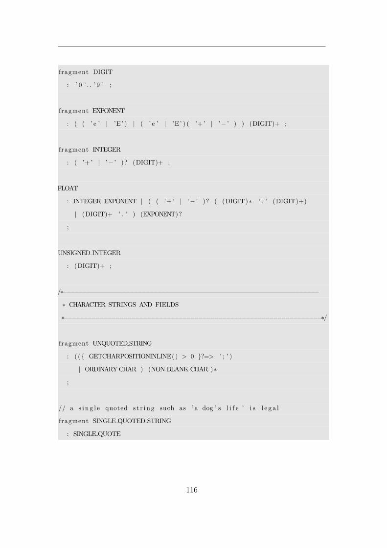
fragment DIGIT

: ’ 0 ’ . . ’ 9 ’ ;

fragment EXPONENT

: ( ( ’ e ’ | ’E ’ ) | ( ’ e ’ | ’E ’ ) ( ’+ ’ | ’− ’ ) ) (DIGIT)+ ;

fragment INTEGER

: ( ’+ ’ | ’− ’ )? (DIGIT)+ ;

FLOAT

: INTEGER EXPONENT | ( ( ’+ ’ | ’− ’ )? ( (DIGIT)∗ ’ . ’ (DIGIT)+)

| (DIGIT)+ ’ . ’ ) (EXPONENT)?

;

UNSIGNED INTEGER

: (DIGIT)+ ;

/∗−−−−−−−−−−−−−−−−−−−−−−−−−−−−−−−−−−−−−−−−−−−−−−−−−−−−−−−−−−−−−−−−−

∗ CHARACTER STRINGS AND FIELDS

∗−−−−−−−−−−−−−−−−−−−−−−−−−−−−−−−−−−−−−−−−−−−−−−−−−−−−−−−−−−−−−−−−−∗/

fragment UNQUOTED STRING

: ( ({ GETCHARPOSITIONINLINE( ) > 0 }?=> ’ ; ’ )

| ORDINARY CHAR ) (NON BLANK CHAR )∗

;

// a s i n g l e quoted s t r i n g such as ’ a dog ’ s l i f e ’ i s l e g a l

fragment SINGLE QUOTED STRING

: SINGLE QUOTE

116

( ( (SINGLE QUOTE NON BLANK CHAR )=>SINGLE QUOTE )

| ANY PRINT CHAR | DOUBLE QUOTE )∗

SINGLE QUOTE

;

fragment DOUBLE QUOTED STRING

: DOUBLE QUOTE

( ( (DOUBLE QUOTE NON BLANK CHAR )=>DOUBLE QUOTE )

| ANY PRINT CHAR | SINGLE QUOTE )∗

DOUBLE QUOTE

;

CHAR STRING

: UNQUOTED STRING | SINGLE QUOTED STRING | DOUBLE QUOTED STRING;

SEMI COLON TEXT FIELD

: ( { GETCHARPOSITIONINLINE( ) == 0 }?=> ’ ; ’ )

( ( ANY PRINT CHAR | SINGLE QUOTE | DOUBLE QUOTE )∗ EOL

( (TEXT LEAD CHAR

( ANY PRINT CHAR | SINGLE QUOTE | DOUBLE QUOTE )∗ )? EOL)∗ )

’ ; ’

;

/∗−−−−−−−−−−−−−−−−−−−−−−−−−−−−−−−−−−−−−−−−−−−−−−−−−−−−−−−−−−−−−−−−−

∗ WHITE SPACE AND COMMENTS

∗−−−−−−−−−−−−−−−−−−−−−−−−−−−−−−−−−−−−−−−−−−−−−−−−−−−−−−−−−−−−−−−−−∗/

COMMENTS

: ( ( ’# ’ (ANY PRINT CHAR | SINGLE QUOTE | DOUBLE QUOTE )∗

117

( EOL | \{ LA(1) == EOF \}? ) )+ )

\{ $channel = HIDDEN; \}

;

// Redef ine t h i s as non−fragment so can be seen by the par s e r

NON BLANK CHAR

: NON BLANK CHAR ;

WHITESPACE

: ( ’\ t ’ | ’ ’ | EOL | ’\u000C ’ )+ ;

118

Appendix C

Additional Information

Courses Attended

• 03/2008 BCA PCG Rietveld Refinement School, Durham University, UK.

• 08/2008 Kyoto Crystallographic Computing School, Japan.

• 03/2009 12th BCA/CCG Intensive Teaching School in X-Ray Structure Anal-

ysis, Durham University, UK.

Conferences Attended

• 04/2008 British Crystallographic Association Spring Meeting, University of

York, UK.

• 08/2008 XXI Congress and General Assembly of the International Union of

Crystallographers, Osaka, Japan.

• 04/2009 British Crystallographic Association Spring Meeting, Loughborough

University, UK.

• 08/2009 25th European Crystallographic Meeting, Istanbul, Turkey.

119

• 11/2009 CCG Autumn Meeting, University of Newcastle-Upon-Tyne, UK.

• 04/2010 British Crystallographic Association Spring Meeting, University of

Warwick, UK.

• 07/2010 American Crystallographic Association Annual Meeting, Chicago,

IL, USA.

• 11/2010 CCG Autumn Meeting, The Royal Society of Edinburgh, UK.

Posters and Oral Presentations Outside Durham

University

• 04/2008 Oral Olex2: The New Molecular Tool. Young Crystallographers

session of the BCA Spring Meeting, York.

• 04/2008 Poster History and metadata in Olex2. BCA Spring Meeting, York.

• 08/2008 Poster Workflow and metadata in Olex2. IUCr Congress, Osaka,

Japan.

• 04/2009 Poster Harnessing the Power of the cctbx with Olex2. BCA Spring

Meeting, Loughborough.

• 08/2009 Poster Harnessing the Power of the cctbx with Olex2. 25th ECM,

Istanbul, Turkey.

• 07/2010 Oral A New Solvent Masking Procedure. ACA Annual Meeting,

Chicago, IL, USA.

• 08/2010 Oral Small Molecule Software for the 21st Century. Lawrence

Berkeley National Laboratory, CA, USA.

120

Publications

• O. V. Dolomanov, L. J. Bourhis, R. J. Gildea, J. A. K. Howard, and H.

Puschmann. OLEX2 : a complete structure solution, refinement and analysis

program. Journal of Applied Crystallography, 42(2):339-341, Apr 2009.

• L. J. Bourhis, R. J. Gildea, O. V. Dolomanov, J. A. K. Howard, and H.

Puschmann. Small molecule toolbox. Newsletter of the IUCr Commission

on Crystallographic Computing, 10:19-32, 2009.

• O. V. Dolomanov, L. J. Bourhis, R. J. Gildea, J. A. K. Howard, and H.

Puschmann. Olex2. Newsletter of the IUCr Commission on Crystallographic

Computing, 10:46-49, 2009.

121

Appendix D

Supplementary Electronic

Materials

D.1 cctbx source code

Source code bundles are provided. The latest source code bundles and instal-

lation instructions can be obtained from http://cci.lbl.gov/build/all.html, where

instructions for accessing the SVN repository can also be found.

Self-extracting cctbx sources for Unix

Under Unix, if Python 2.3 through 2.7 is pre-installed on the target platform,

the smaller cctbx bundle.selfx can be used. However, in general it will be best

to use the cctbx python 271 bundle.selfx file because the installation script will

automatically install a recent Python before proceeding with the installation of

the cctbx modules.

The Unix bundles include a file cctbx install script.csh. This script is known

to work with:

- Linux: any gcc ≥ 3.2 - Mac OS 10.4 or higher with Apple’s compiler

Other Unix platforms will most likely require adjustments of the build scripts.

122

Run the following command in any new, empty directory:

p e r l cctbx bundle . s e l f x

This installs all cctbx modules from scratch. Python 2.3 or higher must be pre-

installed on the target machine. The first python on PATH is used. To install

with a different, specific python, add the full path to the command line, e.g.:

p e r l cctbx bundle . s e l f x / usr / l o c a l / bin /python

Manually building from sources under Windows 2000 or

higher

The cctbx installation requires Visual C++ 8.0 (Visual Studio .NET 2005) or

higher.

To install Python under Windows it is best to use a binary installer from the

Python download page, http://www.python.org/download/. The default choices

presented by the installation wizard are usually fine.

Recent self-contained cctbx sources are available in the self-extracting file

cctbx bundle.exe. To unpack this file in a new, empty directory enter

cctbx bundle . exe

This creates a subdirectory cctbx sources. The installation procedure should

be executed in another directory, e.g.

mkdir c c tbx bu i l d

cd c c tbx bu i l d

C:\python27\python . exe . . \ c c t b x s o u r c e s \ l i b t b x \ c o n f i g u r e . py smtbx iotbx

The last command initializes the cctbx build directory and creates a file set-

paths.bat (among others). This file must be used to initialize a new shell or process

with the cctbx settings

s e tpaths . bat

To compile enter

123

l i b t b x . scons

On a machine with multiple CPUs enter

l i b t b x . scons −j N

where N is the number of CPUs available.

Note that libtbx.scons is just a thin wrapper around SCons. The SCons docu-

mentation applies without modification.

To run some regression tests after the compilation is finished enter::

s e t p a t h s a l l . bat

l i b t b x . python %SCITBX DIST%\ r u n t e s t s . py

l i b t b x . python %CCTBX DIST%\ r u n t e s t s . py −−Quick

The output should show many OK. A Python Traceback is an indicator for

problems.

D.2 Olex2 binaries

Current development builds of Olex2 are provided for Windows, Mac and Linux

platforms.

Windows installation

Run installer.exe alongside the olex2.zip or olex2-x64.zip file to perform offline

installation of the development version of Olex2. The default installation folder

is in in the C:\Program Files\ directory, but you can change that to another

location if you prefer or don’t have access to that area. The different versions will

install into sub-folders called Olex2-1.1, Olex2-1.1-beta etc. Different versions of

Olex2 can be installed next to each other and will operate entirely independently.

124

Mac OS X installation

Unzip the file mac-intel-py26.zip into a new folder, and edit the start script to

point it to the right location of the olex2.app. Then use this start script to launch

Olex2.

Linux installation

The binaries provided should be compatible with most Linux distributions (but

may not be optimised for your machine architecture). We provide Suse 10.1 bina-

ries, which you can find in suse101x32-py26.zip and suse101x64-py26.zip. Unzip

the correct file for your machine and modify the start script inside olex2 folder, to

point to the right location of the executable.

Linux RPMs for several Fedora and Centos versions are kindly provided by

Dr. John Warren. Further information on installing these can be obtained at

http://www.olex2.org/content/folder-linux.

125

References

S. C. Abrahams and E. T. Keve. Normal probability plot analysis of error in mea-

sured and derived quantities and standard deviations. Acta Crystallographica

Section A, 27(2):157–165, Mar 1971. doi: 10.1107/S0567739471000305. 40, 42,

48

P. D. Adams, P. V. Afonine, G. Bunkoczi, V. B. Chen, I. W. Davis, N. Echols,

J. J. Headd, L.-W. Hung, G. J. Kapral, R. W. Grosse-Kunstleve, A. J. McCoy,

N. W. Moriarty, R. Oeffner, R. J. Read, D. C. Richardson, J. S. Richardson,

T. C. Terwilliger, and P. H. Zwart. PHENIX: a comprehensive Python-based

system for macromolecular structure solution. Acta Crystallographica Section

D, 66(2):213–221, Feb 2010. doi: 10.1107/S0907444909052925. 2, 4, 9, 17

P. V. Afonine, R. W. Grosse-Kunstleve, and P. D. Adams. A robust bulk-solvent

correction and anisotropic scaling procedure. Acta Crystallographica Section D,

61(7):850–855, Jul 2005. doi: 10.1107/S0907444905007894. 63

F. H. Allen. The Cambridge Structural Database: a quarter of a million crystal

structures and rising. Acta Crystallographica Section B, 58(3 Part 1):380–388,

Jun 2002. doi: 10.1107/S0108768102003890. 54

F. H. Allen, O. Johnson, G. P. Shields, B. R. Smith, and M. Towler. CIF

applications. XV. enCIFer: a program for viewing, editing and visualizing

CIFs. Journal of Applied Crystallography, 37(2):335–338, Apr 2004. doi:

10.1107/S0021889804003528. 86

E. Aubert and C. Lecomte. Illustrated Fourier transforms for crystallography.

126

REFERENCES

Journal of Applied Crystallography, 40(6):1153–1165, Dec 2007. doi: 10.1107/

S0021889807043622. 59

A. S. Batsanov. Private communication, 2000. 67

A. S. Batsanov. Private communication, 2009. 69

A. S. Batsanov, A. E. Goeta, J. A. K. Howard, A. K. Hughes, and J. M. Malget.

The synthesis of closo- and nido-(aminoalkyl)dicarbaboranes: a re-examination

of contradictory literature reports, crystal structure of [7-H3N(CH2)3-7,8-

c2b9h11]nh2nh2. J. Chem. Soc., Dalton Trans., 12:1820–1826, 2001. doi:

10.1039/B102009I. 68

A. S. Batsanov, R. M. K. Deng, K. B. Dillon, A. E. Goeta, J. A. K. Howard, J. Mel-

drum, P. K. Monks, H. Puschmann, and H. J. Shepherd. Crystal and molecular

structures of some six-coordinate tin(iv) halogeno complexes with phosphorus-

containing ligands. Heteroatom Chemistry, 20(3):136–143, 2009. ISSN 1098-

1071. doi: 10.1002/hc.20525. 67

P. W. Betteridge, J. R. Carruthers, R. I. Cooper, K. Prout, and D. J.

Watkin. CRYSTALS version 12: software for guided crystal structure analy-

sis. Journal of Applied Crystallography, 36(6):1487, Dec 2003. doi: 10.1107/

S0021889803021800. 24, 90

J. M. Bijvoet, A. F. Peerdeman, and A. J. van Bommel. Determination of the

Absolute Configuration of Optically Active Compounds by Means of X-Rays.

Nature, 168(4268):271–272, Aug 1951. doi: 10.1038/168271a0. 33

W. Bluhm. Star (cif) parser. http://pdb.sdsc.edu/STAR/index.html, 2000. 75

S. Bogza, K. Kobrakov, A. Malienko, I. Perepichka, S. Sujkov, M. Bryce,

S. Lyubchik, A. Batsanov, and N. Bogdan. A versatile synthesis of pyra-

zolo [3, 4-c] isoquinoline derivatives by reaction of 4-aryl-5-aminopyrazoles with

aryl/heteroaryl aldehydes: the effect of the heterocycle on the reaction path-

ways. Organic & Biomolecular Chemistry, 3(5):932–940, 2005. ISSN 1477-0520.

65

127

REFERENCES

L. J. Bourhis, R. J. Gildea, O. V. Dolomanov, J. A. K. Howard, and H. Puschmann.

Small molecule toolbox. Newsletter of the IUCr Commission on Crystallographic

Computing, 10:19–32, 2009. 15

L. J. Bourhis, R. J. Gildea, O. V. Dolomanov, J. A. K. Howard, and H. Puschmann.

2011. 58, 64

D. Britton. Estimation of twinning parameter for twins with exactly superimposed

reciprocal lattices. Acta Crystallographica Section A, 28(3):296–297, May 1972.

doi: 10.1107/S0567739472000786. 23, 24

I. D. Brown and I. A. Guzei. Restraints CIF Dictionary. 2011. URL ftp://ftp.

iucr.org/pub/cif core restraints.dic. 81

I. D. Brown and B. McMahon. CIF: the computer language of crystallography.

Acta Crystallographica Section B, 58(3 Part 1):317–324, Jun 2002. doi: 10.1107/

S0108768102003464. 74

M. C. Burla, R. Caliandro, M. Camalli, B. Carrozzini, G. L. Cascarano, L. De Caro,

C. Giacovazzo, G. Polidori, D. Siliqi, and R. Spagna. IL MILIONE: a suite of

computer programs for crystal structure solution of proteins. Journal of Applied

Crystallography, 40(3):609–613, Jun 2007. doi: 10.1107/S0021889807010941. 3

W. Chang and P. E. Bourne. CIF Applications. IX. A new approach for repre-

senting and manipulating STAR files. Journal of Applied Crystallography, 31

(3):505–509, Jun 1998. doi: 10.1107/S0021889897017019. 75

C. A. Christensen, A. S. Batsanov, M. R. Bryce, and J. A. K. Howard. Molec-

ular saddles. 7.1 new 9,10-bis(1,3-dithiol-2-ylidene)-9,10-dihydroanthracene cy-

clophanes: synthesis, redox properties, and x-ray crystal structures of neutral

species and a dication salt. J. Org. Chem., 66(10):3313–3320, 2001. doi:

10.1021/jo001524k. 68

P. Coppens and A. Volkov. The interplay between experiment and theory in

charge-density analysis. Acta Crystallographica Section A, 60(5):357–364, Sep

2004. doi: 10.1107/S0108767304014953. 90

128

REFERENCES

D. Coster, K. S. Knol, and J. A. Prins. Difference in the intensities of x-ray

reflection from the two sides of the 111 plane of zinc blende. Z. Phys., 63:

345–369, 1930. 33

B. Dittrich, M. Strumpel, M. Schafer, M. Spackman, and T. Koritsanszky. Invar-

ioms for improved absolute structure determination of light-atom crystal struc-

tures. Acta Crystallographica Section A: Foundations of Crystallography, 62(3):

217–223, 2006a. ISSN 0108-7673. 90

B. Dittrich, M. Strumpel, M. Schafer, M. A. Spackman, and T. Koritsanszky.

Invarioms for improved absolute structure determination of light-atom crystal

structures. Acta Crystallographica Section A, 62(3):217–223, May 2006b. doi:

10.1107/S0108767306010336. 36

O. V. Dolomanov, L. J. Bourhis, R. J. Gildea, J. A. K. Howard, and H. Puschmann.

OLEX2: a complete structure solution, refinement and analysis program. Jour-

nal of Applied Crystallography, 42(2):339–341, Apr 2009a. doi: 10.1107/

S0021889808042726. 3, 31, 48, 64, 88

O. V. Dolomanov, L. J. Bourhis, R. J. Gildea, J. A. K. Howard, and H. Puschmann.

Age concern - the background. Newsletter of the IUCr Commission on Crystal-

lographic Computing, 10:46–49, 2009b. 1

M. Dusek, V. Petrıcek, M. Wunschel, R. E. Dinnebier, and S. van Smaalen. Re-

finement of modulated structures against X-ray powder diffraction data with

JANA2000. Journal of Applied Crystallography, 34(3):398–404, Jun 2001. doi:

10.1107/S0021889801003302. 24

P. Ellis and H. Bernstein. CBFlib: An API for CBF/imgCIF Crystallographic

Binary Files with ASCII Support, 2001. 75

G. Fermi, M. Perutz, B. Shaanan, and R. Fourme. The crystal structure of human

deoxyhaemoglobin at 1.74 A resolution. Journal of Molecular Biology, 175(2):

159–174, 1984. ISSN 0022-2836. 82

H. D. Flack. On enantiomorph-polarity estimation. Acta Crystallographica Section

A, 39(6):876–881, Nov 1983. doi: 10.1107/S0108767383001762. iii, 22, 34, 89

129

REFERENCES

H. D. Flack and G. Bernardinelli. Reporting and evaluating absolute-structure

and absolute-configuration determinations. Journal of Applied Crystallography,

33(4):1143–1148, Aug 2000. doi: 10.1107/S0021889800007184. 35, 45

G. Friedel. Sur les symtries cristallines que peut rvler la diffraction des rayons X.

C.R. Acad. Sci. Paris, 157:1533–1536, 1913. 32

C. Giacovazzo, H. L. Monaco, G. Artioli, D. Viterbo, G. Ferraris, G. Gilli, G. Zan-

otti, and M. Catti. Fundamentals of Crystallography. Oxford University Press,

2002. 8, 9, 49

N. Godbert, A. S. Batsanov, M. R. Bryce, and J. A. K. Howard. Molecular saddles.

4.1 redox-active cyclophanes by bridging the 9,10-bis(1,3-dithiol-2-ylidene)-9,10-

dihydroanthracene system: synthesis, electrochemistry, and x-ray crystal struc-

tures of neutral species and a dication salt. The Journal of Organic Chemistry,

66(3):713–719, 2001. doi: 10.1021/jo001014q. PMID: 11430087. 65

C. T. Grainger. Pseudo-merohedral twinning. The treatment of overlapped data.

Acta Crystallographica Section A, 25(3):427–434, May 1969. doi: 10.1107/

S0567739469000866. 23, 24

S. Grazulis, D. Chateigner, R. T. Downs, A. F. T. Yokochi, M. Quiros, L. Lut-

terotti, E. Manakova, J. Butkus, P. Moeck, and A. Le Bail. Crystallogra-

phy Open Database – an open-access collection of crystal structures. Jour-

nal of Applied Crystallography, 42(4):726–729, Aug 2009. doi: 10.1107/

S0021889809016690. 75, 82

R. W. Grosse-Kunstleve. Evaluation of different approaches to minimization: full-

matrix and conjugate gradient as implemented in shelx-76 and shelxl-97, lbfgs

and new algorithms under development. Private communication, 2011. 86

R. W. Grosse-Kunstleve and P. D. Adams. On the handling of atomic anisotropic

displacement parameters. Journal of Applied Crystallography, 35(4):477–480,

Aug 2002. doi: 10.1107/S0021889802008580. 7

130

REFERENCES

R. W. Grosse-Kunstleve and P. D. Adams. State of the toolbox: an overview of

the computational crystallography toolbox (cctbx). Comp. Comm. Newsletter,

1, 2003. 4

R. W. Grosse-Kunstleve, N. K. Sauter, N. W. Moriarty, and P. D. Adams.

The Computational Crystallography Toolbox: crystallographic algorithms in a

reusable software framework. Journal of Applied Crystallography, 35(1):126–

136, Feb 2002. doi: 10.1107/S0021889801017824. 4, 63

R. W. Grosse-Kunstleve, P. V. Afonine, and P. D. Adams. cctbx news: Geome-

try restraints and other new features. Newsletter of the IUCr Commission on

Crystallographic Computing, 4:19–36, 2004. 18

J. Haestier. Handling cell-parameter errors in crystallographic data. Jour-

nal of Applied Crystallography, 42(5):798–809, Oct 2009. doi: 10.1107/

S0021889809024376. 30

S. R. Hall and H. J. Bernstein. CIF Applications. V. CIFtbx2: extended tool box

for manipulating CIFs. Journal of Applied Crystallography, 29(5):598–603, Oct

1996. doi: 10.1107/S0021889896006371. 75

S. R. Hall, F. H. Allen, and I. D. Brown. The crystallographic information file

(CIF): a new standard archive file for crystallography. Acta Crystallographica

Section A, 47(6):655–685, Nov 1991. doi: 10.1107/S010876739101067X. 74

W. C. Hamilton. Significance tests on the crystallographic R factor. Acta Crys-

tallographica, 18(3):502–510, Mar 1965. doi: 10.1107/S0365110X65001081. 34

A. P. Hammersley, H. J. Bernstein, and J. D. Westbrook. Image CIF Dictionary

(imgCIF) and Crystallographic Binary File Dictionary (CBF). 2003. URL ftp/

/ftp.iucr.org/pub/cif img.dic. 74

N. K. Hansen and P. Coppens. Testing aspherical atom refinements on small-

molecule data sets. Acta Crystallographica Section A, 34(6):909–921, Nov

1978. doi: 10.1107/S0567739478001886. URL http://dx.doi.org/10.1107/

S0567739478001886. 90

131

REFERENCES

R. Herbst-Irmer and G. M. Sheldrick. Refinement of Twinned Structures with

SHELXL97. Acta Crystallographica Section B, 54(4):443–449, Aug 1998. doi:

10.1107/S0108768197018454. 22

R. Herbst-Irmer and G. M. Sheldrick. Refinement of obverse/reverse twins. Acta

Crystallographica Section B, 58(3 Part 2):477–481, Jun 2002. doi: 10.1107/

S0108768102001039. 22

J. R. Hester. A validating CIF parser: PyCIFRW. Journal of Applied Crystallog-

raphy, 39(4):621–625, Aug 2006. doi: 10.1107/S0021889806015627. 75

F. L. Hirshfeld. Can X-ray data distinguish bonding effects from vibrational

smearing? Acta Crystallographica Section A, 32(2):239–244, Mar 1976. doi:

10.1107/S0567739476000533. 10, 12

R. W. W. Hooft, L. H. Straver, and A. L. Spek. Determination of absolute structure

using Bayesian statistics on Bijvoet differences. Journal of Applied Crystallog-

raphy, 41(1):96–103, Feb 2008. doi: 10.1107/S0021889807059870. iii, 36, 37, 38,

39, 44, 45, 89, 90

R. W. W. Hooft, L. H. Straver, and A. L. Spek. Probability plots based on

Student’s t-distribution. Acta Crystallographica Section A, 65(4):319–321, Jul

2009. doi: 10.1107/S0108767309009908. 42

R. W. W. Hooft, L. H. Straver, and A. L. Spek. Using the t-distribution

to improve the absolute structure assignment with likelihood calculations.

Journal of Applied Crystallography, 43(4):665–668, Aug 2010. doi: 10.1107/

S0021889810018601. 42, 44, 90

J. A. K. Howard and D. J. Watkin. Age concern - the background. Newsletter of

the IUCr Commission on Crystallographic Computing, 10:7–18, 2009. 1

E. R. Howells, D. C. Phillips, and D. Rogers. The probability distribution of X-

ray intensities. II. Experimental investigation and the X-ray detection of centres

of symmetry. Acta Crystallographica, 3(3):210–214, May 1950. doi: 10.1107/

S0365110X50000513. 49

132

REFERENCES

G. B. Jameson. On structure refinement using data from a twinned crystal.

Acta Crystallographica Section A, 38(6):817–820, Nov 1982. doi: 10.1107/

S0567739482001673. 25

JCrystalSoft. FTL-SE. http://jcrystal.com/products/ftlse/index.htm, 2010. viii,

60

Khronos Group. OpenGL the industry standard for high performace graphics.

http://www.opengl.org. 3

Y. Lin. ASTAR: a .NET class library for STAR/CIF manipulation. Jour-

nal of Applied Crystallography, 43(4):916–919, Aug 2010. doi: 10.1107/

S0021889810018145. 75

M. Lutz and A. M. M. Schreurs. Was Bijvoet right? Sodium rubidium (+)-tartrate

tetrahydrate revisited. Acta Crystallographica Section C, 64(8):m296–m299, Aug

2008. doi: 10.1107/S0108270108022415. 33

G. Madariaga. CIF Dictionary for Modulated Structures. 2002. URL ftp://ftp.

iucr.org/pub/cif ms.dic. 74

P. Mallinson. Electron density CIF dictionary. 2003. URL ftp://ftp.iucr.org/pub/

cif rho.dic. 74

P. Murray-Rust. The crystal structure of [Co(NH3)6]4Cu5Cl17: a twinned cubic

crystal. Acta Crystallographica Section B, 29(11):2559–2566, Nov 1973. doi:

10.1107/S0567740873007004. 23, 24

G. Oszlanyi and A. Suto. The charge flipping algorithm. Acta Crystallographica

Section A, 64(1):123–134, Jan 2008. doi: 10.1107/S0108767307046028. 5, 90

L. Palatinus and G. Chapuis. SUPERFLIP – a computer program for the so-

lution of crystal structures by charge flipping in arbitrary dimensions. Jour-

nal of Applied Crystallography, 40(4):786–790, Aug 2007. doi: 10.1107/

S0021889807029238. 3

133

REFERENCES

T. Parr. The Definitive ANTLR Reference: Building Domain-Specific Languages.

Pragmatic Programmers. Pragmatic Bookshelf, first edition, May 2007. ISBN

0978739256. 75, 110

S. Parsons and H. Flack. Precise absolute-structure determination in light-atom

crystals. Acta Crystallographica Section A, 60(a1):s61, Aug 2004. doi: 10.1107/

S0108767304098800. 18, 36, 90

V. Petrıcek and M. Dusek. JANA98, The crystallographic Computing System.

Institute of Physics, Academy of Sciences of the Czech Republic, Praha, Czech

Republic, 2000. 24

S. Picard, P. Gougeon, and M. Potel. Rb4Mo21Se24 containing Mo12 and Mo15

clusters. Acta Crystallographica Section C, 57(4):335–336, Apr 2001. doi: 10.

1107/S0108270100019466. 84

L. Potterton, S. McNicholas, E. Krissinel, J. Gruber, K. Cowtan, P. Emsley, G. N.

Murshudov, S. Cohen, A. Perrakis, and M. Noble. Developments in the CCP4

molecular-graphics project. Acta Crystallographica Section D, 60(12 Part 1):

2288–2294, Dec 2004. doi: 10.1107/S0907444904023716. 2

C. S. Pratt, B. A. Coyle, and J. A. Ibers. Redetermination of the structure of

nitrosylpenta-amminecobalt(iii) dichloride. J. Chem. Soc. A, pages 2146–2151,

1971. doi: 10.1039/J19710002146. 25

Python Software Foundation. Python programming language. http://www.

python.org/. 4, 75, 76

D. Rogers. On the application of Hamilton’s ratio test to the assignment of absolute

configuration and an alternative test. Acta Crystallographica Section A, 37(5):

734–741, Sep 1981. doi: 10.1107/S0567739481001629. 34

D. E. Sands. Transformations of variance-covariance tensors. Acta Crystallograph-

ica, 21(6):868–872, Dec 1966. doi: 10.1107/S0365110X66004092. 27, 29

L. Schroder, D. J. Watkin, A. Cousson, R. I. Cooper, and W. Paulus. CRYSTALS

enhancements: refinement of atoms continuously disordered along a line, on a

134

REFERENCES

ring or on the surface of a sphere. Journal of Applied Crystallography, 37(4):

545–550, Aug 2004. doi: 10.1107/S0021889804009847. 56

D. Schwarzenbach. On uncertainty estimates of crystallographic quantities in-

cluding cell-parameter uncertainties. Journal of Applied Crystallography, 43(6):

1452–1455, Dec 2010. doi: 10.1107/S0021889810039592. 30

SciPy. Scientific tools for python. http://www.scipy.org/. 46

G. Sheldrick. The SHELX-97 Manual. Dept. of Structural Chemistry, Univ. of

Gottingen, Gottingen, Germany, 1997. 9, 12, 13, 14, 18, 24

G. M. Sheldrick. A short history of SHELX. Acta Crystallographica Section A, 64

(1):112–122, Jan 2008. doi: 10.1107/S0108767307043930. 3, 24, 35, 58, 64, 75,

90

A. L. Spek. Single-crystal structure validation with the program PLATON.

Journal of Applied Crystallography, 36(1):7–13, Feb 2003. doi: 10.1107/

S0021889802022112. 3, 40, 56

A. L. Spek. Structure validation in chemical crystallography. Acta Crystallograph-

ica Section D, 65(2):148–155, Feb 2009. doi: 10.1107/S090744490804362X. 86

E. Stanley. The identification of twins from intensity statistics. Journal of Applied

Crystallography, 5(3):191–194, Jun 1972. doi: 10.1107/S0021889872009185. 49,

50

Student. The probable error of a means. Biometrika, 6(1):1–25, 1908. doi: 10.

1093/biomet/6.1.1. 42

B. H. Toby. Powder CIF dictionary. 1998. URL ftp://ftp.iucr.org/pub/cif pd.dic.

74

A. A. Vagin, R. A. Steiner, A. A. Lebedev, L. Potterton, S. McNicholas, F. Long,

and G. N. Murshudov. REFMAC5 dictionary: organization of prior chemical

knowledge and guidelines for its use. Acta Crystallographica Section D, 60(12

Part 1):2184–2195, Dec 2004. doi: 10.1107/S0907444904023510. 74

135

REFERENCES

P. van der Sluis and A. L. Spek. BYPASS: an effective method for the refinement of

crystal structures containing disordered solvent regions. Acta Crystallographica

Section A, 46(3):194–201, Mar 1990. doi: 10.1107/S0108767389011189. iii, 5,

56, 73, 89

J. Waser. Least-squares refinement with subsidiary conditions. Acta Crystallo-

graphica, 16(11):1091–1094, Nov 1963. doi: 10.1107/S0365110X63002929. 7

D. Watkin. Structure refinement: some background theory and practical strategies.

Journal of Applied Crystallography, 41(3):491–522, Jun 2008. doi: 10.1107/

S0021889808007279. 8, 61

J. D. Westbrook, S.-H. Hsieh, and P. M. D. Fitzgerald. CIF Applications. VI.

CIFLIB: an application program interface to CIF dictionaries and data files.

Journal of Applied Crystallography, 30(1):79–83, Feb 1997. doi: 10.1107/

S0021889896008643. 75

S. P. Westrip. publCIF: software for editing, validating and formatting crystal-

lographic information files. Journal of Applied Crystallography, 43(4):920–925,

Aug 2010. doi: 10.1107/S0021889810022120. 86

Wolfram Research, Inc. Mathematica Edition: Version 8.0, 2010. 31

wxWidgets. wxWidgets cross-platform GUI library. http://www.wxwidgets.org.

3

D. S. Yufit and J. A. K. Howard. Cyclopentanone and cyclobutanone. Acta

Crystallographica Section C, 67(3):o104–o106, Mar 2011. doi: 10.1107/

S0108270111004069. 82

W. H. Zachariasen. Dispersion in quartz. Acta Crystallographica, 18(4):714–716,

Apr 1965. doi: 10.1107/S0365110X65001640. 24

P. H. Zwart, R. W. Grosse-Kunstleve, and P. D. Adams. Xtriage and Fest: au-

tomatic assessment of X-ray data and substructure structure factor estimation.

CCP4 Newsletter, 43:contribution 7, 2005. 25

136