Application of Ordinary Kriging Technique to In Situ

Site Characterization

Rojimol, J1, Phanindra, K. B. V. N

2, B. Umashankar

3

1 IIT Hyderabad, Kandi, Sangareddy-502285 2 IIT Hyderabad, Kandi, Sangareddy-502285 3 IIT Hyderabad, Kandi, Sangareddy-502285

Abstract. Application of geostatistical methods to in situ site characterization

has received much attention in the last couple of decades. One of the most pop-

ular and accurate geostatistical method is kriging technique. There are three

types of kriging techniques: simple, ordinary, and universal kriging. This study

has considered developing a generalized ordinary kriging algorithm often pre-

ferred for site characterization. Ordinary kriging assumes the mean of a station-

ary variable as a constant but to be estimated. In kriging, prediction of spatial

variability of a random variable can be obtained using the best fitting semi-

variogram functions. Various semi-variogram models available are exponential,

spherical, and Gaussian. Kriging technique generates a contour map and the er-

ror variance map to infer on the spatial variation of the parameter under consid-

eration. In this study, the clay content parameter from a refinery project area in

Orissa is interpolated using ordinary kriging technique. A generalized

MATLAB code is developed to select the best fitting semi-variogram for the

sample data and to apply ordinary kriging technique and generate the surface

profile. Distribution of clay content values across the region is studied using

prediction surface, and accuracy is checked using error variance profiles. Re-

sults of the analysis are also compared with simulation using ArcGIS based

geo-statistical analyst® and cross-validated using statistical parameters. The

proposed code can be applied to predict various other in situ soil properties in

the field of geotechnical engineering.

Keywords: Ordinary Kriging, Semi-variogram, Site Characterization.

1. Introduction

One of the complex tasks in any major infrastructure project is to handle geotechnical

properties, which are heterogeneous and spatially varying across the domain. Geosta-

tistical techniques that deal with spatial variables to predict the spatial distribution of

observed finite parameters can aid in geotechnical engineering. Geostatistical tech-

niques are classified into two, viz., deterministic and probabilistic (kriging algo-

rithms), based on the underlying functions. Kriging techniques developed by Krige

(1951) and Matheron (1963) solves spatial estimation problems based on least-square

estimators. There are two categories of kriging techniques, namely linear and nonline-

ar. Linear kriging algorithms are based on linear regression technique and are classi-

fied as simple kriging, ordinary kriging, and universal kriging. Simple kriging as-

2

sumes the mean of a stationary variable as a constant and is known prior to kriging,

while ordinary kriging assumes the mean value localized to neighborhood and univer-

sal kriging assumes the mean value to be locally varied with neighborhood. The ad-

vantage being these algorithms are capable of generating prediction confidence/error

variance map along with the prediction surface (Johnston et al., 2001). There are only

a few findings on factors affecting the kriging estimates such as kriging techniques,

sample size, sampling design, and the nature of the data (Asa et al., 2012). This study

aims at developing a reliable code for ordinary kriging by identifying the model sensi-

tive parameters in terms of search neighborhood, underlying semi-variogram func-

tions along with the sample size and various other parameters.

Numerous researchers have demonstrated that kriging algorithms can be used for

geotechnical engineering applications (Soulie et al., 1990; Jaksa, 1993; Rouhani et.

al., 1996; Fenton, 1997; Robinson and Metternicht, 2006; Lenz and Baise, 2007; Ex-

adaktylos, 2008; Samui and Sitharam, 2010; Asa et al, 2012; Rui Yang et al, 2019).

Soulie et al. (1990) have found the value of undrained shear strength (Su) at different

depth using kriging from various borings in B-6 clay in Quebec. They developed

variograms to model the variation in Su values along with both horizontal and vertical

directions. Honjo and Kuroda (1991) used kriging to predict the probability of slope

failure subjected to a fixed driving force. Fenton (1997) has used kriging to calculate

the probability of settlement beneath a footing. Rui Yang et al. (2019) used kriging to

find the best sampling location in case of slopes.

ArcGIS provides various tools (Spatial Analyst® and Geostatistical Analyst®) to

apply geostatistics (Johnston et al., 2001). Even though ArcGIS is a powerful com-

mercial tool for geostatistics, some of the limitations include (a) high cost, (b) lacks

automation in selecting the best semi-variogram model for the experimental data, and

(c) inability to identify and separate the positional outliers from the data set. In addi-

tion to ArcGIS, GStat, and mGStat models are widely available geostatistical tools

with its interface in MATLAB. ASTM D 5923-96 on ‘Site Characterization for Envi-

ronmental Purposes with Emphasis on Soil, Rock, the Vadose Zone and Ground Wa-

ter’ suggests various important factors while applying kriging techniques. Code rec-

ommends that linear geostatistical techniques should be applied only when the soil

data passes normality. In other cases, nonlinear geostatistical techniques should be

applied. This codal provision suggests that if very few spatial outliers are present,

then one can go with ordinary kriging technique. If a large number of spatial outliers

are present, then nonlinear kriging techniques are to be adopted. In addition, there is

no geostatistical tool available specific to geotechnical engineering. This paper aims

at developing a generalized MATLAB ordinary kriging algorithm which can readily

be used by a construction/site manager in generating the optimal surface and error

variance surface of the parameter of interest from the raw spatial data overcoming the

limitation of ArcGIS.

2. Methodology

3

A generalized MATLAB code that uses ordinary kriging algorithm to generate the

prediction and error surfaces for various site parameters was developed in the present

study. The generalized code includes unique functionalities as follows:

2.1 Conversion of co-ordinate system

Global positioning system (GPS) units used for site investigation usually collects the

borehole location in spherical (latitude/longitude) system with respect to an assumed

datum and spheroid. However, for a smaller area of interest, representation in planar

co-ordinate systems is convenient and appropriate (Canters, 2002). The code is devel-

oped to consider the datum and projections corresponding to the geographic location

of the study area, and project into planar co-ordinates.

2.2 Removal of positional outliers

A positional outlier is defined as any observation which positionally deviates by an

excessive amount from other observations (Hawkins 1980). The developed code de-

tects the positional outlier using point density (number of data points per the rectangu-

lar area outlined by the four extreme directional points) approach, by suppressing

each borehole location, one at a time and comparing the point density for each modi-

fied rectangular area (with a limit of 10-15% threshold)

2.3 Test for normality of the data

Graphical methods (Q-Q plots) available in conventional tools are not suitable for

normal test of small samples due to difficulty with the visual comparison. Statistical

based Kolmogorov-Smirnov test which is more preferred is used here (at 5% and 10%

significance levels)

2.4 Generating the experimental semi-variogram

The empirical semi-variogram (Matheron 1972) of the data set is given by:

∑

(1)

where, Z(xi) is the measured value of the parameter at location xi; Z(xi+h) is the

measured value of the parameter at its neighbor xi h ; |h| is the average distance

between the pairs of data points; and N(|h|) is the number of pairs of data points that

belongs to the distance interval represented by h. An ideal semi-variogram first in-

creases non-linearly with distance and levels off at a certain distance (range) and after

some point, distance will have no effect on the variability in the parameter.

2.5 Fitting the best theoretical model

4

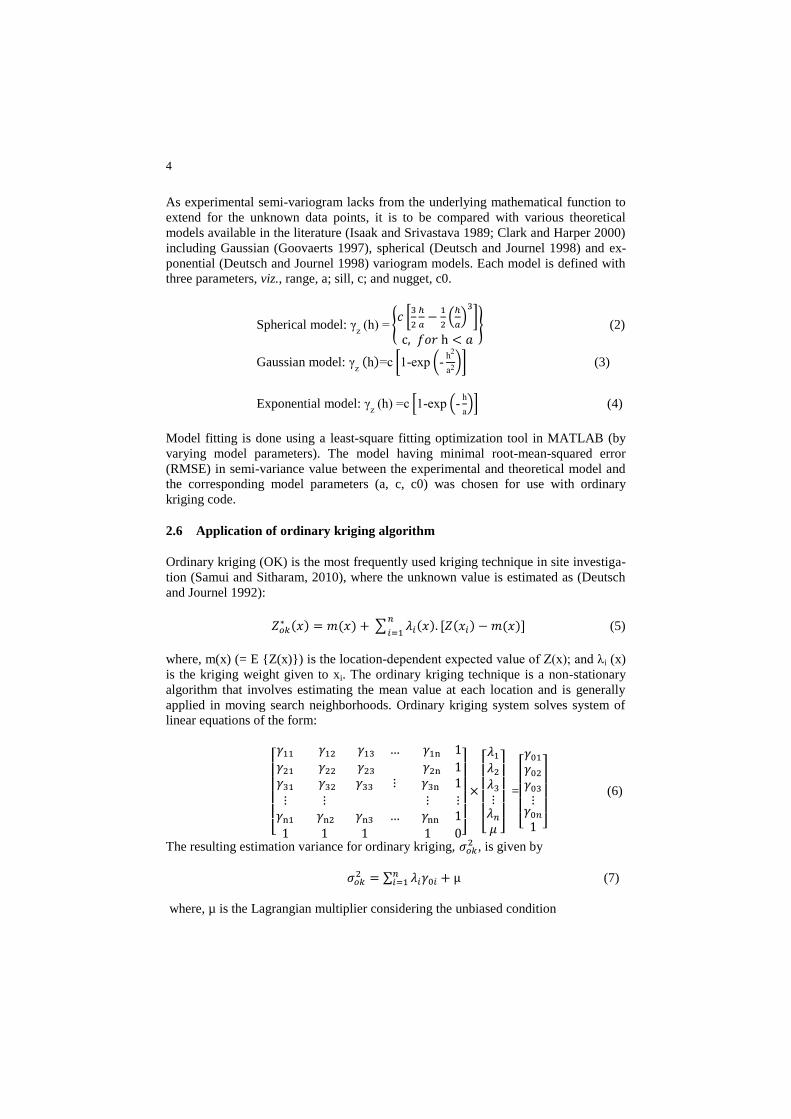
As experimental semi-variogram lacks from the underlying mathematical function to

extend for the unknown data points, it is to be compared with various theoretical

models available in the literature (Isaak and Srivastava 1989; Clark and Harper 2000)

including Gaussian (Goovaerts 1997), spherical (Deutsch and Journel 1998) and ex-

ponential (Deutsch and Journel 1998) variogram models. Each model is defined with

three parameters, viz., range, a; sill, c; and nugget, c0.

Spherical model: h {

[

(

)

]

} (2)

Gaussian model: h [ - xp (-

h

)] (3)

Exponential model: h * - xp (-

h

)+ (4)

Model fitting is done using a least-square fitting optimization tool in MATLAB (by

varying model parameters). The model having minimal root-mean-squared error

(RMSE) in semi-variance value between the experimental and theoretical model and

the corresponding model parameters (a, c, c0) was chosen for use with ordinary

kriging code.

2.6 Application of ordinary kriging algorithm

Ordinary kriging (OK) is the most frequently used kriging technique in site investiga-

tion (Samui and Sitharam, 2010), where the unknown value is estimated as (Deutsch

and Journel 1992):

∑

(5)

where, m(x) (= E {Z(x)}) is the location-d p nd nt xp t d v lu of Z x ; nd λi (x)

is the kriging weight given to xi. The ordinary kriging technique is a non-stationary

algorithm that involves estimating the mean value at each location and is generally

applied in moving search neighborhoods. Ordinary kriging system solves system of

linear equations of the form:

[

]

[

]

=

[

]

(6)

The resulting estimation variance for ordinary kriging, , is given by

∑

(7)

where, µ is the Lagrangian multiplier considering the unbiased condition

5

2.7 Factors affecting ordinary kriging algorithm precision

Factors affecting algorithm precision are specified limiting radius, and minimum and

maximum values of neighbor points. Those points lying farther are ignored based on

Tobl r’s l w of geography, which says that as the distance between the points in-

creases, properties are less co-related in space. This methodology is called searching

neighborhood. The developed MATLAB code calculates the best suitable neighbor-

hood combination factors for each grid location. While estimating the kriging

weights, some values are observed to be negative as some points are "shadowed" by

closer points. Negative weights can affect the accuracy of prediction by increasing or

decreasing the prediction estimate/ estimation variance. The program also eliminates

the points with the most negative weight, and recomputes the weights and repeat the

process until the value becomes positive. These all factors improve the precision of

developed code.

3. Case Study: Paradip Refinery Project, Orissa

3.1 Site description

The refinery site (Fig. 1) is located approximately 7 km South West of Paradip Port

on the North bank of the River, Kansarbatia, and is located near Paradip port in

Jagatsingpur district of Orissa, India. Geographic location of the site is 21o 07’ . 7”

N latitude, and 90O 8’ 0. 8” E. longitud . The geographical coverage area of the

region is about 3549 acres (14.96 km2). There were total fifty-seven (57) boreholes

drilled to conduct extensive site investigation. Ground surface was slightly uneven as

boreholes drilled in the area under study differed by 0.63 m to 4.78 m, due to part of

the area having been filled. During the investigation, it was observed that the filled up

area constitutes yellowish brown fine to medium sand to a depth of about 3.0m, fol-

lowed by a layer of soft to firm clay followed by sand strata which is loose at the top,

becoming medium dense to occasionally dense. Alternate layers of (medium dense to

very dense) sand and (stiff to hard) clay up to the maximum depth 100m underlie

these deposits.

6

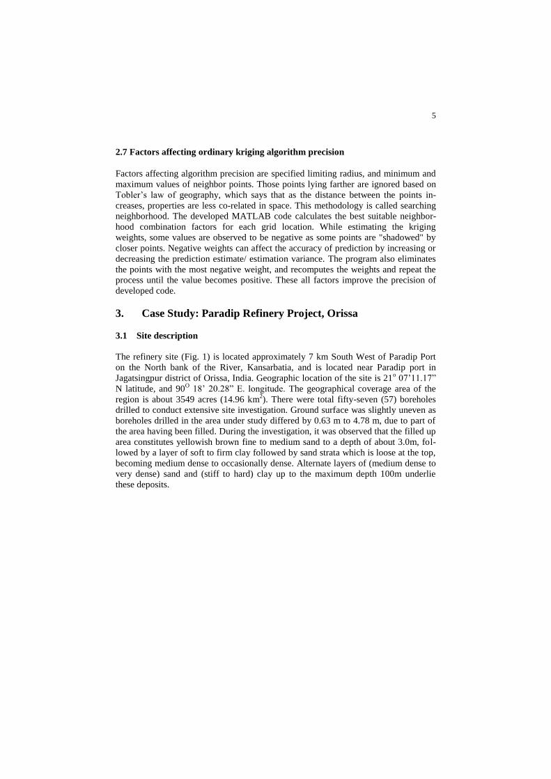
Fig. 1. Schematic of Paradip refinery project site with boreholes

3.2 Spatial outlier removal

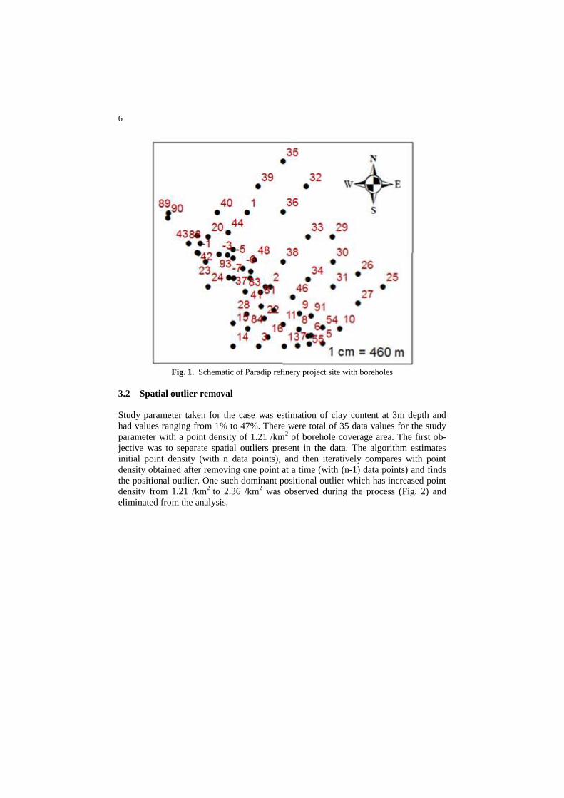
Study parameter taken for the case was estimation of clay content at 3m depth and

had values ranging from 1% to 47%. There were total of 35 data values for the study

parameter with a point density of 1.21 /km2 of borehole coverage area. The first ob-

jective was to separate spatial outliers present in the data. The algorithm estimates

initial point density (with n data points), and then iteratively compares with point

density obtained after removing one point at a time (with (n-1) data points) and finds

the positional outlier. One such dominant positional outlier which has increased point

density from 1.21 /km2

to 2.36 /km2 was observed during the process (Fig. 2) and

eliminated from the analysis.

7

Fig. 2. Spatial distribution of data considered in the analysis

3.3 Normality check

A hypothesis based Kolmogorov-Smirnov test that suits for smaller samples was ap-

plied with the algorithm as Q-Q plots in ArcGIS tools cannot accurately check for the

normality. Test results show that distribution follows the normal distribution at a sig-

nificance level of 5%.

3.4 Semi-variogram and model fitting

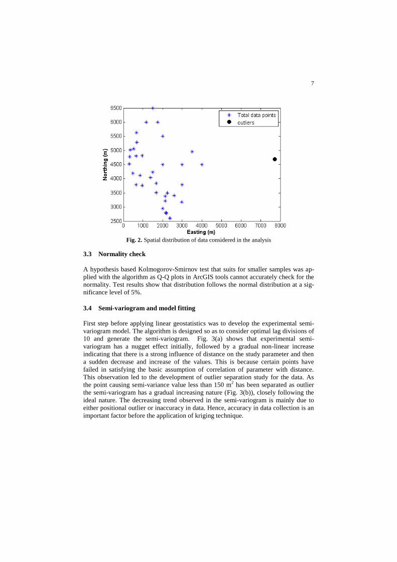
First step before applying linear geostatistics was to develop the experimental semi-

variogram model. The algorithm is designed so as to consider optimal lag divisions of

10 and generate the semi-variogram. Fig. 3(a) shows that experimental semi-

variogram has a nugget effect initially, followed by a gradual non-linear increase

indicating that there is a strong influence of distance on the study parameter and then

a sudden decrease and increase of the values. This is because certain points have

failed in satisfying the basic assumption of correlation of parameter with distance.

This observation led to the development of outlier separation study for the data. As

the point causing semi-variance value less than 150 m2 has been separated as outlier

the semi-variogram has a gradual increasing nature (Fig. 3(b)), closely following the

ideal nature. The decreasing trend observed in the semi-variogram is mainly due to

either positional outlier or inaccuracy in data. Hence, accuracy in data collection is an

important factor before the application of kriging technique.

8

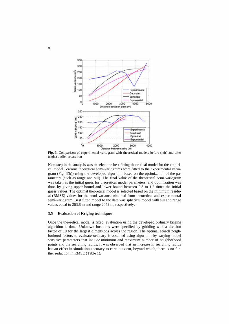
Fig. 3. Comparison of experimental variogram with theoretical models before (left) and after

(right) outlier separation

Next step in the analysis was to select the best fitting theoretical model for the empiri-

cal model. Various theoretical semi-variograms were fitted to the experimental vario-

gram (Fig. 3(b)) using the developed algorithm based on the optimization of the pa-

rameters (such as range and sill). The final value of the theoretical semi-variogram

was taken as the initial guess for theoretical model parameters, and optimization was

done by giving upper bound and lower bound between 0.8 to 1.2 times the initial

guess values. The optimal theoretical model is selected based on the minimum residu-

al (RMSE) values for the semi-variance obtained from theoretical and experimental

semi-variogram. Best fitted model to the data was spherical model with sill and range

values equal to 263.8 m and range 2059 m, respectively.

3.5 Evaluation of Kriging techniques

Once the theoretical model is fixed, evaluation using the developed ordinary kriging

algorithm is done. Unknown locations were specified by gridding with a division

factor of 10 for the largest dimensions across the region. The optimal search neigh-

borhood factors to evaluate ordinary is obtained using algorithm by varying model

sensitive parameters th t in lud minimum and maximum number of neighborhood

points and the searching radius. It was observed that an increase in searching radius

has an effect in simulation accuracy to certain extent, beyond which, there is no fur-

ther reduction in RMSE (Table 1).

9

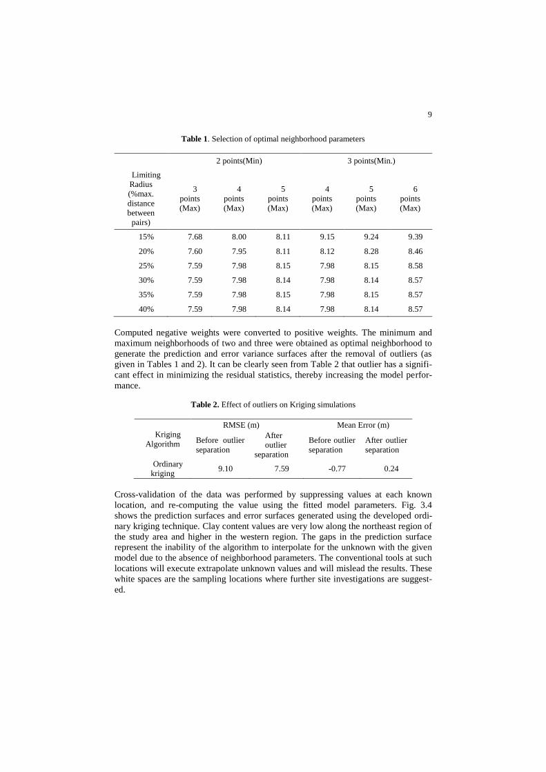
Table 1. Selection of optimal neighborhood parameters

2 points(Min) 3 points(Min.)

Limiting

Radius

(%max.

distance

between

pairs)

3

points

(Max)

4

points

(Max)

5

points

(Max)

4

points

(Max)

5

points

(Max)

6

points

(Max)

15% 7.68 8.00 8.11 9.15 9.24 9.39

20% 7.60 7.95 8.11 8.12 8.28 8.46

25% 7.59 7.98 8.15 7.98 8.15 8.58

30% 7.59 7.98 8.14 7.98 8.14 8.57

35% 7.59 7.98 8.15 7.98 8.15 8.57

40% 7.59 7.98 8.14 7.98 8.14 8.57

Computed negative weights were converted to positive weights. The minimum and

maximum neighborhoods of two and three were obtained as optimal neighborhood to

generate the prediction and error variance surfaces after the removal of outliers (as

given in Tables 1 and 2). It can be clearly seen from Table 2 that outlier has a signifi-

cant effect in minimizing the residual statistics, thereby increasing the model perfor-

mance.

Table 2. Effect of outliers on Kriging simulations

Kriging

Algorithm

RMSE (m) Mean Error (m)

Before outlier

separation

After

outlier

separation

Before outlier

separation

After outlier

separation

Ordinary

kriging 9.10 7.59 -0.77 0.24

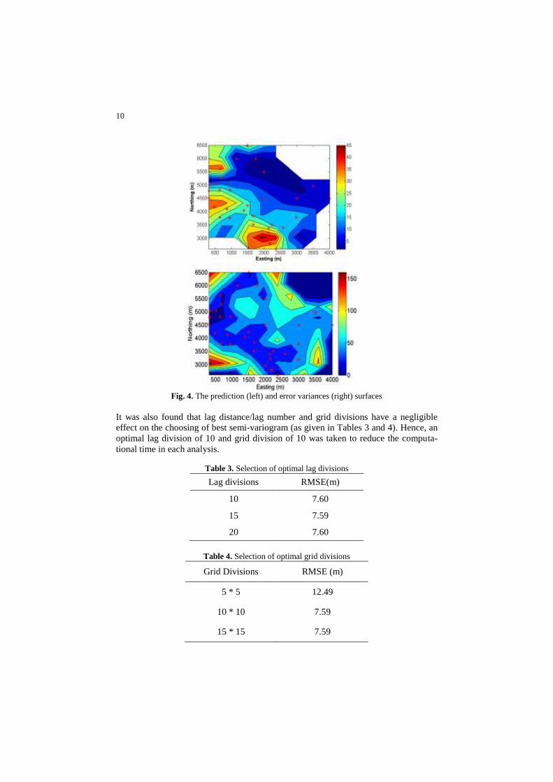
Cross-validation of the data was performed by suppressing values at each known

location, and re-computing the value using the fitted model parameters. Fig. 3.4

shows the prediction surfaces and error surfaces generated using the developed ordi-

nary kriging technique. Clay content values are very low along the northeast region of

the study area and higher in the western region. The gaps in the prediction surface

represent the inability of the algorithm to interpolate for the unknown with the given

model due to the absence of neighborhood parameters. The conventional tools at such

locations will execute extrapolate unknown values and will mislead the results. These

white spaces are the sampling locations where further site investigations are suggest-

ed.

10

Fig. 4. The prediction (left) and error variances (right) surfaces

It was also found that lag distance/lag number and grid divisions have a negligible

effect on the choosing of best semi-variogram (as given in Tables 3 and 4). Hence, an

optimal lag division of 10 and grid division of 10 was taken to reduce the computa-

tional time in each analysis.

Table 3. Selection of optimal lag divisions

Lag divisions RMSE(m)

10 7.60

15 7.59

20 7.60

Table 4. Selection of optimal grid divisions

Grid Divisions RMSE (m)

5 * 5 12.49

10 * 10 7.59

15 * 15 7.59

11

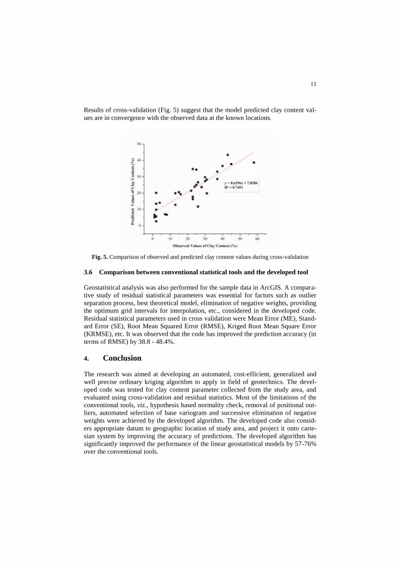
Results of cross-validation (Fig. 5) suggest that the model predicted clay content val-

ues are in convergence with the observed data at the known locations.

Fig. 5. Comparison of observed and predicted clay content values during cross-validation

3.6 Comparison between conventional statistical tools and the developed tool

Geostatistical analysis was also performed for the sample data in ArcGIS. A compara-

tive study of residual statistical parameters was essential for factors such as outlier

separation process, best theoretical model, elimination of negative weights, providing

the optimum grid intervals for interpolation, etc., considered in the developed code.

Residual statistical parameters used in cross validation were Mean Error (ME), Stand-

ard Error (SE), Root Mean Squared Error (RMSE), Kriged Root Mean Square Error

(KRMSE), etc. It was observed that the code has improved the prediction accuracy (in

terms of RMSE) by 38.8 - 48.4%.

4. Conclusion

The research was aimed at developing an automated, cost-efficient, generalized and

well precise ordinary kriging algorithm to apply in field of geotechnics. The devel-

oped code was tested for clay content parameter collected from the study area, and

evaluated using cross-validation and residual statistics. Most of the limitations of the

conventional tools, viz., hypothesis based normality check, removal of positional out-

liers, automated selection of base variogram and successive elimination of negative

weights were achieved by the developed algorithm. The developed code also consid-

ers appropriate datum to geographic location of study area, and project it onto carte-

sian system by improving the accuracy of predictions. The developed algorithm has

significantly improved the performance of the linear geostatistical models by 57-76%

over the conventional tools.

12

References

1. Krige, D. G.: A statistical approach to some basic mine valuation problems on the Witwa-

tersrand. J. Chem. Metall. Min. Soc. South Africa, 52(6), 119–139 (1951).

2. Matheron, G.: Principles of geostatistics. Econ. Geol., 58(8), 1246–1266 (1963b).

3. D. M. Hawkins.: Identification of Outliers. Biometrical Journal, 29 (2), (1980) 198.

4. E. H. Isaaks and R. M. Srivastava. An introduction to applied geostatistics, Oxford Univer-

sity Press, New York, (1989) 561.

5. Soulié, M., Montes, P., and Silvestri, V.: Modelling spatial variability of soil parameters.

Can. Geotech. J 27, 617–630 (1990).

6. Y. Honjo. and K. Kuroda. A new look at fluctuating geotechnical data for reliability de-

sign, soils and foundations. Jpn. Soc. Soil Mech. Found. Eng. 31 (1), (1991) 110–120.

7. Rouhani, S., Srivastava, R.M., Desbarats, A.J., Cromer, M.V. and Johnson, A.I.: Geosta-

tistics for Environmental and Geotechnical Applications, ASTM, Philadelphia, 3–31

(1996).

8. Jaksa, M. B., Brooker, P. I. and Kaggwa, W. S.: Modelling the Spatial Variability of the

Undrained Shear Strength of Clay Soils Using Geostatistics. Proceedings of fifth Int. Geo-

statistics Congress, Wollongong, 1284–1295 (1997).

9. Fenton, G. A.: Probabilistic methods in geotechnical engineering, ASCE Geotechnical

Safety and Reliability Committee (1997).

10. P. Goovaerts. Geostatistics for natural resources evaluation. Oxford University Press. New

York, (1997) 483.

11. C. V. Deutsch and A. G. Journel. GSLIB. Geostatistical software library and user’s guide.

Oxford University Press, New York, (1998) 369.

12. K. Johnston, J. M. Ver Hoef, K. Krivoruchko and N. Lucas. Using ArcGIS-geostatistical

analyst. GIS by ESRI. Redlands. USA, (2001).

13. Clark, I., and Harper, W. Practical geostatistics 2000. Ecosse. North America Llc, (2002)

14. F. Canters. Small scale map projection design. Taylor and Francis, London, (2002) 343.

15. Robinson, T. P., and Metternicht, G.: Testing the performance of spatial interpolation

techniques for mapping soil properties. Comput Electron. Agric., 50(2), 97–108 (2006).

16. Lenz, J. A., and Baise, L. G.: Spatial variability of liquefaction potential in regional map-

ping using CPT and SPT data. Soil Dyn. Earthquake Eng., 27(7), 690–702 (2007).

17. Exadaktylos, G., Stavropoulou, M., Xiroudakis, G., de Broissia and M., Schwarz, H. A:

Spatial estimation model for continuous rock mass characterization from the specific ener-

gy of a TBM. Rock Mech. Rock Eng., 41(6), 797–834 (2008).

18. P. Samui and T. Sitharam.: Site Characterization Model Using Artficial Neural Network

and Kriging. Int. J. Geomech.10 (5), (2010) 171-180.

19. E. Asa, M. Saafi, J. Membah, and A. Billa.: Comparison of Linear and Nonlinear Kriging

Methods for Characterization and Interpolation of Soil Data. J. Comput. Civ. Eng., 26 (1),

(2012) 11-18.

20. Rui Yang, Jinsong Huang, D.V. Griffiths, Jinhui Li, Daichao Sheng.: Importance of soil

property sampling location in slope stability assessment, Canadian Geotechnical Journal,

56(3), 335-346 (2019).

21. ASTM. Standard Guide for Selection of Kriging Methods in Geostatistical Site Investiga-

tions. D5923-96. West Conshohocken, PA: ASTM International (2010b)