application of probe vehicle data for real-time traffic state estimation and short-term travel

Nanthawichit, C., Nakatsuji, T., and Suzuki, H.

Application of Probe Vehicle Data for Real-Time Traffic State Estimation and Short-Term Travel Time Prediction on a Freeway

Chumchoke Nanthawichit Graduate Student Transportation and Traffic Systems Graduate School of Engineering, Hokkaido University Kita-13, Nishi-8, Kita-ku, Sapporo 060-8628, Japan. Tel: +81-11-706-6822 Fax: +81-11-706-6216 Email: [email protected] Takashi Nakatsuji Associate Professor Transportation and Traffic Systems Graduate School of Engineering, Hokkaido University Kita-13, Nishi-8, Kita-ku, Sapporo 060-8628, Japan. Tel: +81-11-706-6215 Fax: +81-11-706-6216 E-mail: [email protected] Hironori Suzuki Research Engineer Safety & ITS Research Division Japan Automobile Research Institute 2530 Karima, Tsukuba, Ibaraki, 305-0822 Japan Tel: +81-298-56-0874 Fax: +81-298-56-0874 Email: [email protected] Submission Date: November 14, 2002. Word Count: 5890(Text)+1500(6 Figures)=7390

TRB 2003 Annual Meeting CD-ROM Paper revised from original submittal.

Nanthawichit, C., T. Nakatsuji, and H. Suzuki 1

ABSTRACT

Traffic information from probe vehicles has great potential for improving the estimation accuracy of traffic situations, especially where no traffic detector is installed. A method for dealing with probe data along with conventional detector data to estimate traffic states is proposed in this paper. The probe data was integrated into the observation equation of the Kalman filter, in which state equations are represented by a macroscopic traffic flow model. Estimated states were updated with information from both stationary detectors and probe vehicles. The method was tested under several traffic conditions based on hypothetical data, giving considerably improved estimation results compared to those estimated without probe data. Finally, the application of the proposed method was extended to the estimation and short-term prediction of travel time. Travel times were obtained indirectly through the conversion of speeds estimated/predicted by the proposed method. Experimental results show that the performance of travel time estimation/prediction is comparable to those of some existing methods.

Keywords: traffic states, travel time, estimation, prediction, probe vehicles, macroscopic traffic flow model, Kalman filter

INTRODUCTION

Reliable traffic information is essential for the development of efficient traffic control and management strategies. Real-time traffic information is utilized for various purposes, such as dynamic route guidance, incident detection, freeway ramp metering control, and the operation of variable message signs. Traffic information can be obtained by several traffic detection devices installed on a road network. However, it is costly and unreasonable to be aware of the traffic situation throughout an entire network using only fixed sensors. A traffic flow simulation model for describing traffic phenomena is a key element in overcoming this difficulty. In general, a traffic management scheme or a route guidance system deals with a large-scale network. A macroscopic model describing the traffic states in an aggregate manner is one of the tools for real-time applications due to its simplicity of traffic flow description and its computational efficiency. Although every macroscopic model has its own deficiencies as discussed in, for example, (1), (2), and (3), several techniques were introduced to compensate for these deficiencies. One such technique, the Kalman filtering technique (KFT), has been integrated into macroscopic models for the real-time estimation of traffic states. Cremer (4), Payne et al. (5), Pourmoallem et al. (6), and Suzuki and Nakatsuji (7) applied the KFT as a feedback method to update the estimated traffic states on a freeway. Nahi and Trivedi (8) proposed the relationship between traffic counts and traffic states and updated the states using the KFT. In these studies, observed traffic data were taken only from fixed vehicle detectors, however with long separation between successive detectors, estimation results will probably deteriorate. In order to estimate traffic states more accurately, traffic information from additional sources might be one solution. With its ability to cover a road network, the probe vehicle technique has great potential in this respect.

Uplink data transmitted by probe vehicles has recently been receiving considerable interest within the modern surveillance system. In such a system, probe vehicles are taken as moving sensors traveling in a traffic flow, whereas conventional detectors, such as inductive loops, are treated as fixed sensors installed only at a limited number of locations. Under such circumstances, probe data would be useful in providing traffic information from links where no conventional detectors are installed. A sufficiently large number of probe vehicles should reasonably represent the traffic conditions experienced; the effect of the level of market penetration on the reliability of probe data has been discussed in several studies (e.g., (9), (10), and (11)). However, so far, the applications for probe vehicle data are still limited. Most studies, such as (9), (10), (12), and (13), have focused on using probe data directly for travel time detection. Some authors (e.g., (9), and (14)) have proposed incident detection algorithms using probe data, and some (e.g., (13)) have discussed the potential of using probe vehicles as sources of O-D information.

So far, very few studies have realized the potential of using probe data to estimate the traffic state of flow, density and speed. Sanwal and Walrand (9) suggested that probe data could be used to estimate traffic state variables, and proposed an algorithm for estimating speed using the Bayesian approach. Recently, Cathey and Dailey (15) proposed a method using transit vehicles as probes for estimating the time series of vehicle locations and speeds. They updated the vehicle position, speed, and acceleration using the KFT. The system equations they used were taken from individual vehicle motion. Their method treats probe vehicles as only an alternative source of traffic data, other than a fixed detector, i.e., a combination of both sources of data was not considered. In addition, apart from average speed, no interest has been paid to the estimation of the other fundamental traffic flow variables of traffic density and traffic volume. Thus it should be useful to develop the formulation for



estimating traffic states (i.e., density, space mean speed and traffic volume) using the combination of traffic data from both stationary detectors and probe vehicles.

Apart from the fundamental traffic state variables, travel time is another important piece of information for Intelligent Transportation Systems. It is widely used as a criterion to determine the minimum cost path in the route guidance of dynamic traffic assignment problems. It is also used directly as information for supporting driver decisions by means of changeable message signs, in-vehicle guidance systems, or radio broadcasting. Several approaches to predict travel time have been proposed, including statistical models (e.g., (12) and (16)) such as time series and autoregressive models, and artificial neural networks (e.g., (17) and (18)). Even though there are many studies for which probe data were used as sources of travel time, very few studies, apart from, for example Chen and Chien (12) who applied travel time data from probe vehicles to update the predicted travel time using an autoregressive function with the KFT, have used probe data for predicting future travel time. Given such a lack of research, it would be interesting to know how effective travel time prediction based on traffic state variables predicted using probe vehicle data would be.

The objective of this study is to propose a method for integrating probe vehicle data into fixed detector data to estimate traffic states on a freeway. The KFT is applied to update the state variables estimated by a macroscopic model. Firstly, the formulation of the proposed method, which considers how to treat the observation variables for the KFT in order to overcome the inconsistency of the observation data, will be presented. Then, the methodology will be examined using several sets of hypothetical data under different traffic conditions. The performance of the proposed method to estimate travel time will also be examined. Finally, a method to predict short-term travel time will be proposed, as a byproduct of traffic state prediction. The prediction results will be compared with the results from one of the effective existing methods.

TRAFFIC STATE ESTIMATION

Macroscopic Traffic Flow Model

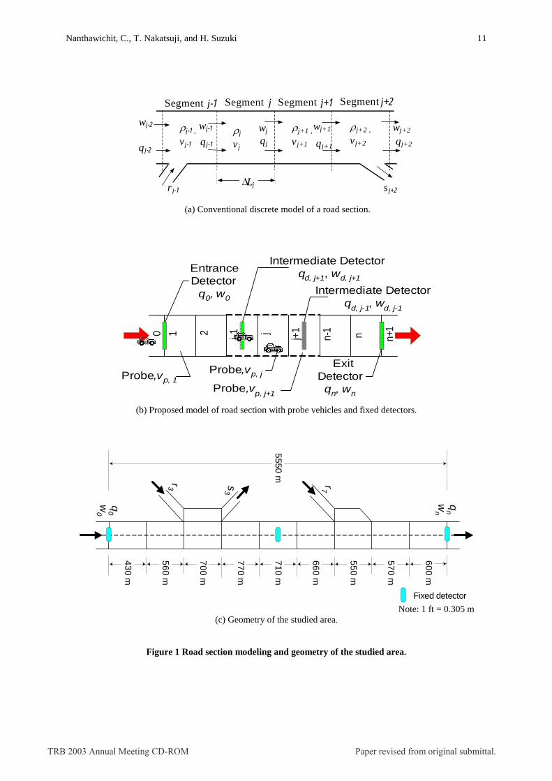
The macroscopic traffic flow model of Payne (19) was selected to apply in this study due to its simplicity in integrating with other techniques including the KFT. It should be noted that this study is not aimed at selecting the best macroscopic model. Moreover, it is not clear that a good result could be guaranteed using a highly complicated model for every situation. Figure 1(a) shows a space-time discreted freeway section, where each segment is �Lj long. It is divided on the assumption that the traffic state is homogeneous within each segment. Equations (1) to (3) describe the discrete form using the explicit finite difference approximation of Payne’s macroscopic model. � � � � � �

� �tjjjjj

jj srqqLttt ��

�

��

�11 �� (1)

� � � � � ��

� � ��

��

��

�

��

� �

��

�

��

�

��

��

�

�

� t

tt

Lttvtvtv

Lttvtvttvtv

j

jj

jj

jjjj

jjjejj

11

11 (2)

� � � � � �� ttvttvtq jjjjj 111��

�� (3)

The macroscopic traffic variables in the model were defined as follows: �j(t) : density of segment j at time t vj(t) : space mean speed of segment j at time t qj(t) : flow rate at the boundary point between segments j and j+1 at time t wj(t) : time mean speed at the boundary point between segments j and j+1 at time t rj(t) : entry flow rate at ramp of segment j at time t sj(t) : exit flow rate at ramp of segment j at time t �t is the time increment; �j is the number of lanes in segment j; ve(.) is the speed at equilibrium state, which can be obtained from the density-speed relationship; and �� , and � are model parameters. Equation (3) reflects the fact that the states of both neighboring segments may affect the volumes determined at the edge of each segment, as suggested by Cremer (4). ��is a weighting parameter ranging from 0 to 1.

Existing Method for Applying the KFT together with a Macroscopic Model

The KFT is a method for adjusting the state variables by the available measurement data. It has been applied in several studies (e.g., (4), (5), (6), and (7)) to estimate traffic states in real-time. Traffic states are first estimated by the macroscopic model. Then, as the system receives the observations, the estimated state variables are



adjusted according to the KFT algorithm. The adjustment of the state variables in proportion to the difference between the observed and estimated values of the observation variables is the core of the KFT.

In the above studies ((4), (6) and, (7)) where measurement data can be obtained from fixed detectors only, traffic density and space mean speed are treated as the state variables, x(t)=(�,v)(t), whereas traffic volumes, q, and spot speeds, w, are treated as the observation variables, y(t)=(q,w)(t). Equation (1) and Equation (2), are treated as state equations, while observation equations consist of a relationship between traffic volume and state variables, as in Equation (3), and a relationship between spot speed and state variables which might be set as the following (4):

� � � � � � � �tvtvtw jjj 11�

�� (4)

where � is the same weighting parameter as used in Equation (3).

To formulate the KFT, white noise errors were induced in both state and observation equations:

� � � �� ttt �� xf1x (5) � � � �� ttt �� xgy (6)

where (t) and (t) are noises representing the modeling errors and measurement errors respectively. They are assumed to be uncorrelated with zero mean. Next, the state and observation equations are linearized around the nominal solution � �tx~ , using Taylor’s expansion. The system equations become:

� � � �� txbtxtAtttt ��

�� xtx

xfxf1x~ (7)

� � � �� ttdtxtCtttt ��

�� x~tx

xg

xgy~ (8)

The dimension of linearization matrix A is nn 22 � , while that of matrix C is nm 22 � . n is the total number of road segments, and m the total number of observation points. � �tx~ and � �tx are the estimated state vectors before and after adjusting with the actual measurement data, y(t), respectively.

The state estimates can be adjusted according to the correction steps of the KFT as follows:

�� step 1 estimate state variables for the current step, t: � � � �� 1xfx~ �� tt �� step 2 calculate error matrix of � �tx~ at time t: � � � � � � � � �� 1A1P1AM tttt T �� step 3 calculate Kalman gain matrix at time t: � � � � � � � � � � � �� 1CMCCMK �

�� tttttt TT �� step 4 estimate observation variables at time t: � � � �� tt x~gy~ � �� step 5 update estimated state variables: � � � � � � � � � �� ttttt y~yKx~x �� step 6 update error matrix of � �tx : � � � � � � � � � �ttttt MCKMP �� step 7 then set 1�� tt and repeat all the steps until the required simulation time is reached.��

� and � are covariance matrices of �(t) and �(t), respectively.

Integration of Probe Data into the State Estimation

Probe data

Generally, there are three possible approaches by which probe vehicles can transmit traffic information. 1. Space-based: probe vehicles transmit traffic information to roadside devices as they pass observation points.

This type of data could be obtained from a beacon-based probe system, an electronic toll tag system, or an automatic license plate recognition system.

2. Time-based: probe data are reported at every specific time instant regardless of the position of the probe vehicle, and could be obtained from a GPS-based system or a beacon-based system.

3. Event based: traffic information is reported when a particular event occurs, for example, traffic accident reports from drivers by cellular phone.

In this study, the second approach was adopted, as it has a higher potential for providing the data from different locations in an entire network, the first approach being more or less the same as a fixed sensor in which data can be obtained from certain locations.



Adjustment in Observation variables of the KFT

The traffic information from probe vehicles that would be applied as an additional observation variable is the average probe speed, because speed is the only information in probe reports that directly appears in the macroscopic model. To make it possible to combine detector and probe speeds into one observation variable in each segment, a road section was modeled, as shown in Figure 1(b), so that fixed detectors (if any) were located at approximately the middle of a segment (except for the detectors at the entrance and exit points of the road section). Moreover the influence of neighboring segments in the calculation of the observation variables can be avoided. This is what differs from the conventional approach mentioned earlier, in which all detectors are located at segment boundaries. Here, one could assume that, at a certain segment j, the observed speed from the fixed detector, wd,j, is the observation variable of the space mean speed of the segment, and the observed volume from the fixed detector, qd,j, is the observation variable of the segment flow (not the flow at boundary).

In this study, it was assumed that probe vehicles could submit their speed along with their current position, regardless of where they were. At every time step, the probe data were sorted by their location as determined from which segment the data were transmitted. Generally, probe data may not be available in all segments for every time step. As a result, the number of observation variables from probes could vary with time. For the segments where both detector and probe data were available, a data fusion technique was required for combining the data from different sources. In this study, for simplicity’s sake, a weighted average of speed from both data sources was used. Weighting factor of 0.5 was assigned to both sources of data. In fact, this factor should be selected based on the reliability of data from each source. Sensitivity analysis of weighting factor, as well as the application of other data fusion techniques would be studied further.

Observation variables and observation equations for each segment, or even the same segment in each time step, may be different depending on the fixed detector locations and the presence of probe vehicles. The observation equations can be divided into three groups:

1. The observation equations at the entrance and exit detectors: As the segments 0, and n+1 are dummy segments, we assumed there is no effect from these segments in estimating entrance and exit observation variables.

q0 = �1v1 (9) w0 = v1 (10) qn = �nvn (11) wn = vn (12)

2. The observation equations for segments that have a supplementary fixed detector: If additional fixed detectors are available in certain segments between the entrance and exit detectors, traffic volume and speed data from these detectors can be used as additional observation variables. As detectors are located at about the middle of each segment, one might assume that the average speed measured at the detectors is equal to the space mean speed of the segments, wd,j = vd,j. Thus, the observation equations for the supplementary detectors are

qd,j = �jvj (13) vd,j = vj (14)

where j identifies the number of segments with a fixed detector. vdj is the observed speed from the detector, in cases where no probe data is available, while the integrated speed from both fixed detector and probe vehicle data are used at a certain time step when probe data are also available.

3. The observation equation for segments with no fixed detector: In a certain time step when probe data are available, the average of probe speeds obtained in each segment is considered to be an observation variable for the space mean speed.

vp,h = vh (15)

where vp,h is the observed speed from the probe vehicles; and h identifies a detector-less segment with probe data.

The method proposed features the ability to deal with inconsistencies in observation data. According to the considerations above, the total number of observation variables is changeable with time. At a certain time step t, the number of observation variables is equal to 4+2m+p0(t). p0(t) denotes the number of segments where only probe data are available and m is the number of segments with a fixed detector. Accordingly, the dimension



of matrix C reduces to � �� nmtpm 224 �� and that of the covariance matrix of the observation variable noises, �� becomes � �� mtpmmtpm �� 2424 .

TRAVEL TIME ESTIMATION AND PREDICTION

Travel Time Estimation

Segment Travel Time

Travel time at a certain instant might be estimated using the average speed from boundary detectors, or directly obtained from spatial-based probe vehicles. However, if one can estimate speeds for the whole network, travel time in a certain segment could be simply converted from the estimated speed as the following equation.

ttj(t)=Lj/vj(t) (16)

ttj(t) is the travel time of segment j at time interval t. Lj denotes the length of segment j.

Path Travel Time

Path travel time can be determined by a simple sum of the travel times of the segments in a path, or a progressive sum, where the exiting time for each segment depends on the time experienced during all downstream segments of the interested one. Equation 17 shows the recursive formula for the progressive path travel time.

� � � � � �� tTttttTtT siisisi ,1,1, �� (17)

Ti,s(t) denotes the path travel time from segment i arriving at destination s at time step t. We defined travel time at the destination point to make it possible to estimate/update using observation data at every time step in real-time. If the path travel time were defined at the origin point, to estimate it, one would have to wait until the interested vehicles reached their destination.

Short-term Prediction

The travel time in the near future can be predicted by applying a predicted speed instead of the estimated one in Equation (16). Thus, the traffic state has to be predicted first. Traffic state prediction is determining the state at a specific target interval in the future, in contrast to estimation, which defines the state at the current step. In this study the prediction interval was selected to be 3 minutes. That is the states are predicted every 3 minutes. It should be noted that the prediction interval is different from the simulation interval. The simulation interval (10 seconds in this study) is the time duration for one estimation/updating step of the macroscopic model and KFT.

To predict short-term traffic states in real time, two parallel modules of estimation as mentioned in the previous section were performed simultaneously. The first module (referred to as the updating model) receives the new observation data and updates the estimation results at every time step. The second module serves for prediction purposes. At every time step, the prediction module is carried out using the prediction inputs, i.e., the predicted observations are required. In this study, to make it simple, the averages of the observation values from the previous prediction step (the last 3 minutes) were used as the input values for the most recent step. The same values were applied until the simulation time reached the next prediction step. At the first simulation step of each prediction interval, all traffic variables in the prediction module were replaced by the ones from the updating module to make the predictions follow a real-time estimation profile.

NUMERICAL EXPERIMENTS

Traffic Data

A 5,550 m (18,197 ft) road section, as shown in Figure 1(c), was modeled emulating the road section of the Yokohane Line of the Metropolitan Expressway in Tokyo, Japan, in an inbound direction between Namamugi Junction and the Taishi Ramp. The road section is divided into nine segments ranging from 400 m (1,311 ft) to 800 m (2,622 ft) with two on-ramps and one off-ramp.

As the availability of probe data in real-world is still limited, simulation software, INTEGRATION (20), after careful calibration and validation with real traffic data, was used to generate traffic data (both observation and reference data). INTEGRATION has various features suitable for ITS applications, including



the capability to generate fixed detector data and probe vehicle data. Simulation makes it possible to control the conditions of data including the percentage of probe vehicles, inflow and outflow volumes, and incident conditions, etc.

Four cases of 3-hour data, as presented in Figure 2, were generated to test the proposed method.

�� Case A: a low-density case. �� Case B: same inflow volume as case A with an incident blocking 1 to 0.5 lanes, from the 90th minute to the

105th minute. �� Case C: low to high density �� Case D: same inflow as case C with the incident as in case B. It was assumed that, if available, probe data could be obtained from anywhere in the study network at any specific interval. Both probe data and fixed detector data can be transmitted to the traffic control center in real-time. To reduce fluctuation, the data were aggregated in a 3-minute interval for both the fixed detectors and probe vehicles data. As a large aggregate interval would diminish the dynamic of the traffic, in the real-world practice, the aggregate interval should be properly selected according to the purpose of data application.

Performance Indices

In order to evaluate the performance of the estimations, error indices based on the deviations of the estimated results from the references were calculated. Two types of indices used in this study, including a root mean square error (RMSE), and a mean absolute relative error (MARE), have the following forms:

� ��

��

N

iii zz

NRMSEz

1

2ˆ1 (18)

��

�

�

N

i i

ii

zzz

NMAREz

1

ˆ1 (19)

N denotes the total number of reference outputs used for comparison. Here, N is equal to the number of segments multiplied by the number of time steps; zi denotes the actual value of the reference variable;

iz denotes the corresponding estimation outputs.

Traffic State Estimation

In the numerical experiment of state estimation, the road section was assumed to have three fixed detectors located at the entrance and exit boundaries and at the middle of segment 5, as depicted in Figure 1(c). For each data case, estimation results from four scenarios, differing in their estimation technique and the level of traffic information, were compared. �� Scenario 1 (S1): macroscopic model only; �� Scenario 2 (S2): macroscopic model with the KFT using the data from a fixed detector in segment 5; �� Scenario 3 (S3): macroscopic model with the KFT using the probe data; �� Scenario 4 (S4): macroscopic model with the KFT using both data from probe vehicles and the

supplementary fixed detector

Based on sensitivity analysis in our previous study (11), a market penetration of 3% was assumed for S3 and S4. The most apparent conclusion that can be drawn from the results summarized in Figure 3 is that the methods using probe data (S3, and S4) provide superior results to those that did not use probe data. The estimation error can be reduced notably. Overall, S4 provides the best results for all cases. It reduces the RMSE in volume by about 20-40%, and improves speed and density estimation by 70-85% compared to the estimation results from the pure macroscopic model (S1). The estimation of S4 is relatively precise as all error indices are small (0.03-0.04 for the MARE of volume, 0.03-0.06 for the MARE of speed, and 0.04-0.07 for the MARE of density). Moreover, less than 20% of the total estimated results have an error over 10% of actual values. S3 provides slightly poorer results than S4 does; however if the number of supplementary detectors increases, one may expect the more deviated results of S3 and S4. In the same way, if only stationary detector data are used, as in S2, to provide the estimation accuracy on the same level as S3 and S4, the denser detecting points are required. In general, the KFT contributes noticeably to the improvement of estimation accuracy. Especially for density and speed, the error can be reduced notably. Deterioration may occur in volume estimation (such as S2 and S3 of case C), however it is not significant as the difference in the MARE is very small.



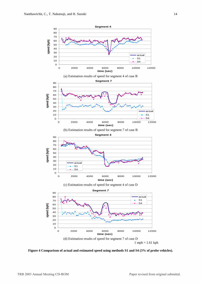
Figure 4 shows the speed variation at segments 4 and 7 of cases B and D estimated using S1 and S4. The profiles of the estimated speeds using S4 accurately follow the actual ones, even in the abrupt change regions as shown around the time step of 5,400 to 6,300 seconds when the incident occurs. On the other hand, the macroscopic model (S1) sometimes fails to capture the real traffic flow in cases as (1) it is too slow to respond to the dynamics of traffic flow as shown in Figure 4(a) and 4(c); (2) in some segments (e.g., segment 7 shown in Figure 4(b) and 4(d)), it might absolutely fail to represent the actual conditions, i.e., the estimation can not return to the correct profile once it deviates.

Travel Time Estimation and Prediction

Travel Time Estimation

Travel time estimation can be carried out once the estimated states are available. To examine the performance of travel time estimation using the speed obtained from the proposed method, the estimated results were compared with those of the other methods. The methods used in this analysis are: �� The proposed method, same as S4 in the previous section, using the macroscopic model and the KFT, which

employs the observation data from both detectors and probe vehicles, denoted as MKFT. �� Time-based probe data (TP): travel time is derived from probe speed as Equation 16. �� Detector data: use boundary speed to calculate travel time as:

� ��

��

��

��

twtwLttt

BA

112

(20)

wA and wB denote the detector speed of consecutive detectors. Three different configurations of detector number and locations were examined:

(1) DT-3: 3 detectors at the entrance and exit of the road section and at the exit of segment 5; (2) DT-5: 5 detectors at the entrance and exit of the road section and at the exit of segments 3, 4, and 7. (3) DT-10: 10 detectors at every segment boundary.

�� Space-based probe data (SP): directly observe travel time between probe reading stations (1) SP-3: 3 probe reading stations at the same location as DT-3 (2) SP-5: 5 probe reading stations at the same location as DT-5 (3) SP-10: 10 probe reading stations at the same location as DT-10

Figures 5(a) and 5(b) summarize the estimation results for the cases of 3% and 1% probe vehicles on the freeway, respectively. In almost all cases, except case B with 3% probe vehicles, the path travel times estimated using the proposed method is better than those estimated by only time-based probe data, which serves as one of the observation data in the proposed method. The proposed method presents better results than the DT method with a small number of detectors in the incident cases (B and D). The DT method gives a good estimation if a large numbers of detectors are installed. The estimation deteriorates drastically in cases where an incident occurs even when 5 detectors are used. That is the DT method is very sensitive to incidents if the detectors are not installed densely. With the same number of detectors the proposed method performs better than the DT method for most cases, except case C of 1% probe vehicles. Compared with the SP method, the proposed method generally gives slightly poorer results than those of SP-10 and SP-5, however with a small proportion of probe vehicles (1%) the proposed method becomes better than the SP method in high-density cases (C and D). Overall, the proposed method could reasonably provide comparable estimates of travel time compared to the other methods aiming specifically to estimate only travel time.

Short-term Travel Time Prediction

The prediction method proposed by (12) using an autoregressive function with the KFT (referred to as AKFT) was selected to compare the prediction results with those of the proposed method. In the AKFT method, both state and observation variables are the travel times. Historical data were used to determine the transition parameter that relates the state variable to the observation variable. In this study, cases A and C were treated as the historical data for cases B and D, respectively, as they have exactly the same inflow pattern. For cases B and D, assuming there were 3% of probe vehicles in the network, one step of the 3-minute-ahead travel times were predicted using the two methods mentioned above.

The results in Figures 6(a) and 6(b) show high conformity between prediction and actual path travel times. The MARE of path travel times for both cases is very small (0.03 for case B, and 0.04 for case D). The



fractions of prediction values that deviate over 10% of actual values are less than 0.02 for case B, and less than 0.08 for case D. Compared with the AKFT method, the proposed method provides slightly better results for both cases B and D, as shown in Figure 6(c). Experimental results confirm the ability of using estimated/predicted traffic state variables to predict travel time.

CONCLUSION

In this paper, a method for treating probe vehicle data together with fixed detector data in order to estimate the traffic state variables of traffic volume, space mean speed and density was proposed. The method used a macroscopic model along with the Kalman filtering technique (KFT). The traffic states described by the macroscopic model were adjusted according to the KFT algorithm. The special features of the proposed method are: �� It can treat both conventional fixed detector data and probe vehicle data in a unified manner, regardless of

the observation conditions. �� It can handle the inconsistencies in the probe vehicle data (i.e., the probe data may not be available for the

whole simulation period in a certain segment).

The method was verified with several sets of hypothetical traffic data. Four different scenarios according to the estimation method and available traffic data were examined for a single freeway section. The results of state estimation showed that the method using both fixed detector and probe data provides the smallest errors. The estimation errors can be reduced significantly (70-85% for speed and density) compared to those estimated using the macroscopic model only. With a high network covering data obtained from probe vehicles, the proposed method can capture the traffic dynamics without any incident information, even when the traffic conditions change abruptly.

In addition, we suggested the possibility of using estimated/predicted states to estimate/predict travel time. A method to predict the short-term horizon of state variables by using parallel estimation modules (one for updating and one for prediction) was also proposed. Estimated path travel times were compared with three conventional methods. Overall, the proposed method could provide reasonably comparable estimates of travel time compared to the other methods that specifically aim to estimate only travel time. The proposed travel time prediction method also works well compared to one of the autoregression methods. In summary, both errors from travel time estimation and prediction are small, i.e., a MARE below 0.04. Experimental results confirm that the proposed method can provide reasonable estimation not only for traffic states but also, as a byproduct of traffic state estimation, travel time can be effectively estimated and predicted. Moreover, it should have the potential to be applied to other issues such as the identification of level of service, and delay time etc.

What has been found in this study is encouraging for dynamic traffic state estimation. Both the macroscopic model and the numerical technique adopted in this study were very simple. Thus, a highly complex model might not be necessary if available traffic data were able to cover most parts of a network. However, the findings have been validated only for a single freeway section. For the further analysis, the proposed method should be applied to diverse road configurations, particularly to a large network. In addition, as this study assumed that the probe data could be obtained perfectly (i.e., there is no consideration on the unreliability of data such as the data error from communication devices, or unavailable data when probe vehicles pass the signal obstructed area), and the effect of the biased data due to individual willingness of probe drivers was neglected, field experiments to determine the feasibility of the proposed method should be conducted. The conclusion drawn from this study still requires supporting real-world data.

ACKNOWLEDGMENTS

Traffic data contributed by the Metropolitan Expressway was greatly appreciated.

REFERENCES

1. Daganzo, C.: Requiem for Second-order Fluid Approximations of Traffic Flow, Transportation. Research, Vol.29B, No.4, 1995, pp.277-286.

2. Michalopoulos, P.G., P. Yi, and A.S. Lyrintzis. Continuum Modelling of Traffic Dynamics for Congested Freeways, Transportation. Research, Vol.27B, No.4, 1993, pp.315-332.

3. Lebacque, J.P., and J.B. Lesort. Macroscopic Traffic Flow Models: A Question of Order, Proceedings of the 14th International. Symposium on Transportation and Traffic Theory, Jerusalem, Israel, 1999, pp.3-25.



4. Cremer, M. Der Verkehrsflu� auf Schnellstra�en, Springer-Verlag, New York, 1979. 5. Payne, H.J., Brown, D., and Cohen, S.L.: Improved Techniques for Freeway Surveillance, In Transportation

Research Record 1112, TRB, National Research Council, Washington, D.C., 1987, pp.52-60. 6. Pourmoallem, N., T. Nakatsuji, and A. Kawamura. A Neural-Kalman Filtering Method for Estimating

Traffic States on Freeways, Journal of Infrastructure Planning and Management, No.569/IV-36, JSCE, 1997, pp.105-114.

7. Suzuki, H., T. Nakatsuji. A New Approach to Estimate Freeway OD Travel Time Based on Dynamic Traffic States Estimation Using Feedback Estimator, Journal of Infrastructure Planning and Management, No.695/IV-54, JSCE, 2002, pp.137-148.

8. Nahi, N.E., and A.N. Trivedi, Recursive Estimation of Traffic Variables: Section Density and Average Speed. Transportation Science, Vol.7, 1973, pp.269-286.

9. Sanwal, K. K., and J. Walrand. Vehicles as Probes. California PATH Working Paper UCB-ITS-PWP-95-11, Institue of Transportation Studies, University of California, Berkley, 1995.

10. Sen, A., P.V. Thakuriah, X.Q. Zhu, and A. Karr. Frequency of Probe Reports and Variance of Travel Time Estimates, Journal of Transportation Engineering, Vol.123, No.4, 1997, pp.209-297.

11. Nanthawichit, C., T. Nakatsuji, and H. Suzuki. Dynamic Estimation of Traffic States on a Freeway Using Probe Vehicle Data, submitted to Journal of Infrastructure Planning and Management, JSCE, 2002.

12. Chen, M., and S. Chien. Dynamic Freeway Travel Time Prediction Using Probe Vehicle Data: Link-based vs. Path-based. In Transportation Research Board 1768, TRB, National Research Council, Washington, D.C., 2001, pp.157-161.

13. Van Aerde, M., B. Hellinga, L. Yu, and H. Rakha. Vehicle Probes as Real-time ATMS Sources of Dynamic O-D and Travel Time Data. Large Urban Systems – Proceedings of the ATMS Conference, St. Petersberg, Florida, 1993, pp.207-230.

14. Sethi, V., N. Bhandari, F.S. Koppelman, and J.L. Schofer. Arterial Incident Detection Using Fixed Detector and Probe Vehicle Data, Transportation Research, Vol.3C, No.2, 1995, pp.99-112.

15. Cathey, F.W., and D.J. Dailey. Transit Vehicles as Traffic Probe Sensors. Transportation Research Board the 81st Annual Meeting (CD-ROM), Washington, D.C., 2002.

16. D’Angelo, M.P., H.M. Al-Deek, and M.C. Wang. Travel-time prediction for freeway corridors. In Transportation Research Record 1676, TRB, National Research Council, Washington, D.C., 1999, pp.184-191.

17. Park, D.J., and L.R. Rilett.: Forecasting Multiple-period freeway link travel times using modular neural networks. In Transportation Research Record 1617, TRB, National Research Council, Washington, D.C., 1998, pp.163-170.

18. Van Lint, H., S.P. Hoogendoorn, and H.J. van Zuylen. Freeway Travel Time Prediction with State-Space Neural Networks. Transportation Research Board the 81st Annual Meeting (CD-ROM), Washington, D.C., 2002.

19. Payne, H.J. Models of Freeway Traffic and Control. Simulation Councils Proceedings Series: Mathematical Models of Public Systems, Vol.1, No.1, 1971, pp.51-61.

20. Rakha, H. INTEGRATION Release 2.30 for Windows: User’s Guide-Volumes 1 and 2, M. Van Aerde & Assoc., Ltd., 2001.



LIST OF FIGURES

FIGURE 1 Road section modeling and geometry of the studied area. FIGURE 2 Simulation data (speed). FIGURE 3 Errors in state estimation for different scenarios for a freeway with 3% probe vehicles. FIGURE 4 Comparison of actual and estimated speed using methods S1 and S4 (3% of probe vehicles). FIGURE 5 Comparison of the results of path travel time estimation using different methods. FIGURE 6 Travel time prediction results for a freeway with 3% probe vehicles.



Segment j-1 Segment j+2 Segment j+1Segment j

q j-1 q j-2 � j-1 , v j-1

�Ljrj-1 sj+2

w j-2 w j-1 qj

�j

vj

wj

qj+1

�j+1 , vj+1

wj+1

q j+2 �j+2 , vj+2

w j+2

(a) Conventional discrete model of a road section.

EntranceDetector

q0, w0

ExitDetector

qn, wn

Intermediate Detectorqd, j-1, wd, j-1

1 2 j j+1j-1 n-1 n0 n+1

Probe,vp, 1Probe,vp, j

Probe,vp, j+1

Intermediate Detectorqd, j+1, wd, j+1

(b) Proposed model of road section with probe vehicles and fixed detectors.

q0

w0

qn

wn

r3 s3

r7

600 m

5550 m

570 m

550 m

430 m

560 m

700 m

770 m

710 m

660 m

Fixed detector Note: 1 ft = 0.305 m

(c) Geometry of the studied area.

Figure 1 Road section modeling and geometry of the studied area.



180

720

1260

1800

2340

2880

3420

3960

4500

5040

5580

6120

6660

7200

7740

8280

8820

9360

9900

1044

0

1

3

5

7

9 segm

ent

Case A

0-10 10-20 20-30 30-40 40-5050-60 60-70 70-80 80-90 90-100

180

720

1260

1800

2340

2880

3420

3960

4500

5040

5580

6120

6660

7200

7740

8280

8820

9360

9900

1044

0

1

3

5

7

9

segm

ent

Case B

0-10 10-20 20-30 30-40 40-5050-60 60-70 70-80 80-90 90-100

180

720

1260

1800

2340

2880

3420

3960

4500

5040

5580

6120

6660

7200

7740

8280

8820

9360

9900

1044

0

1

3

5

7

9 segm

ent

Case C

0-10 10-20 20-30 30-40 40-5050-60 60-70 70-80 80-90 90-100

180

720

1260

1800

2340

2880

3420

3960

4500

5040

5580

6120

6660

7200

7740

8280

8820

9360

9900

1044

0

13579

time (sec)se

gmen

t

Case D

0-10 10-20 20-30 30-40 40-5050-60 60-70 70-80 80-90 90-100

Speed in Kph

1 mph = 1.61 kph

Figure 2 Simulation data (speed).



0

50

100

150

200

250300

350

400

450

REM

SEq

(vph

)

caseS1 220 276 270 344S2 145 297 423 407S3 178 218 300 253S4 141 171 217 208

A B C D

(a) RMSE of estimated volume (vph)

0.00

0.05

0.10

0.15

0.20

0.25

0.30

0.35

0.40

MA

REq

caseS1 0.053 0.059 0.050 0.062S2 0.029 0.044 0.066 0.067S3 0.037 0.043 0.049 0.047S4 0.028 0.032 0.035 0.037

A B C D

(d) MARE of estimated volume

0

2

4

6

8

10

12

14

16

18

RM

SEv

(kph

)

caseS1 14.9 16.2 13.2 14.5S2 6.6 9.6 6.7 7.2S3 2.4 3.0 3.7 3.6S4 2.4 2.9 3.5 3.6

A B C D

(b) RMSE of estimated speed (kph)

0.00

0.05

0.10

0.15

0.20

0.25

0.30

0.35

0.40

MA

REv

caseS1 0.211 0.232 0.235 0.261S2 0.084 0.121 0.103 0.117S3 0.031 0.039 0.059 0.058S4 0.030 0.039 0.057 0.057

A B C D

(e) MARE of estimated speed

05

101520253035404550

RM

SE��

(vpk

)

caseS1 26.2 32.9 41.6 47.9S2 9.5 19.6 29.1 30.0S3 4.0 7.3 12.0 12.4S4 3.6 6.4 10.9 11.7

A B C D

(c) RMSE of estimated density (vpk)

1 mph = 1.61 kph 1 vpm = 0.62 vpk

Figure 3 Errors in state estimation for different scenarios for a freeway with 3% probe vehicles.

0.00

0.05

0.10

0.15

0.20

0.25

0.30

0.35

0.40

RM

SE��

caseS1 0.318 0.365 0.324 0.370S2 0.105 0.143 0.145 0.150S3 0.047 0.059 0.074 0.075S4 0.041 0.051 0.067 0.069

A B C D

(f) MARE of estimated density



Segment 4

0

10

20

30

40

50

60

70

80

90

0 2000 4000 6000 8000 10000 12000time (sec)

spee

d (k

ph)

actualS1S4

(a) Estimation results of speed for segment 4 of case B

Segment 7

0

10

20

30

40

50

60

70

80

90

0 2000 4000 6000 8000 10000 12000time (sec)

spee

d (k

ph)

actualS1S4

(b) Estimation results of speed for segment 7 of case B

Segment 4

0

10

20

30

40

50

60

70

80

90

0 2000 4000 6000 8000 10000 12000

time (sec)

spee

d (k

ph)

actualS1S4

(c) Estimation results of speed for segment 4 of case D

Segment 7

0

10

20

30

40

50

60

70

80

90

0 2000 4000 6000 8000 10000 12000time (sec)

spee

d (k

ph)

actualS1S4

(d) Estimation results of speed for segment 7 of case D

1 mph = 1.61 kph

Figure 4 Comparison of actual and estimated speed using methods S1 and S4 (3% of probe vehicles).



(a) RMSE of estimated path travel time for a freeway with 3% probe vehicles

(b) RMSE of estimated path travel time for a freeway with 1% probe vehicles

Figure 5 Comparison of the results of path travel time estimation using different methods.

0

10

20

30

40

50

60

TP 4.3 8.0 28.0 22.8

MKFT 3.8 10.8 22.4 19.8

DT-3 6.6 31.5 32.5 53.9

DT-5 5.5 33.8 25.0 33.3

DT-10 3.5 10.6 16.7 18.1

SP-3 5.7 8.3 24.3 22.3

SP-5 3.7 7.1 22.8 22.2

SP-10 3.0 4.4 18.0 17.7

A B C D

RM

SET

(sec

)

case0

10

20

30

40

50

60

TP 4.3 8.0 28.0 22.8

MKFT 3.8 10.8 22.4 19.8

DT-3 6.6 31.5 32.5 53.9

DT-5 5.5 33.8 25.0 33.3

DT-10 3.5 10.6 16.7 18.1

SP-3 5.7 8.3 24.3 22.3

SP-5 3.7 7.1 22.8 22.2

SP-10 3.0 4.4 18.0 17.7

A B C D

RM

SET

(sec

)

case

0

10

20

30

40

50

60

TP 6.8 18.8 45.2 34.8

MKFT 6.1 17.1 36.3 28.7

DT-3 6.6 31.5 32.5 53.9

DT-5 5.5 33.8 25.0 33.3

DT-10 3.5 10.6 16.7 18.1

SP-3 8.8 11.5 43.9 40.3

SP-5 7.0 11.3 39.2 34.3

SP-10 5.3 7.8 37.5 33.0

A B C D

RM

SET

(sec

)

case0

10

20

30

40

50

60

TP 6.8 18.8 45.2 34.8

MKFT 6.1 17.1 36.3 28.7

DT-3 6.6 31.5 32.5 53.9

DT-5 5.5 33.8 25.0 33.3

DT-10 3.5 10.6 16.7 18.1

SP-3 8.8 11.5 43.9 40.3

SP-5 7.0 11.3 39.2 34.3

SP-10 5.3 7.8 37.5 33.0

A B C D

RM

SET

(sec

)

case

0

10

20

30

40

50

60

TP 4.3 8.0 28.0 22.8

MKFT 3.8 10.8 22.4 19.8

DT-3 6.6 31.5 32.5 53.9

DT-5 5.5 33.8 25.0 33.3

DT-10 3.5 10.6 16.7 18.1

SP-3 5.7 8.3 24.3 22.3

SP-5 3.7 7.1 22.8 22.2

SP-10 3.0 4.4 18.0 17.7

A B C D

RM

SET

(sec

)

case0

10

20

30

40

50

60

TP 4.3 8.0 28.0 22.8

MKFT 3.8 10.8 22.4 19.8

DT-3 6.6 31.5 32.5 53.9

DT-5 5.5 33.8 25.0 33.3

DT-10 3.5 10.6 16.7 18.1

SP-3 5.7 8.3 24.3 22.3

SP-5 3.7 7.1 22.8 22.2

SP-10 3.0 4.4 18.0 17.7

A B C D

RM

SET

(sec

)

case0

10

20

30

40

50

60

TP 4.3 8.0 28.0 22.8

MKFT 3.8 10.8 22.4 19.8

DT-3 6.6 31.5 32.5 53.9

DT-5 5.5 33.8 25.0 33.3

DT-10 3.5 10.6 16.7 18.1

SP-3 5.7 8.3 24.3 22.3

SP-5 3.7 7.1 22.8 22.2

SP-10 3.0 4.4 18.0 17.7

A B C D

RM

SET

(sec

)

case

0

10

20

30

40

50

60

TP 6.8 18.8 45.2 34.8

MKFT 6.1 17.1 36.3 28.7

DT-3 6.6 31.5 32.5 53.9

DT-5 5.5 33.8 25.0 33.3

DT-10 3.5 10.6 16.7 18.1

SP-3 8.8 11.5 43.9 40.3

SP-5 7.0 11.3 39.2 34.3

SP-10 5.3 7.8 37.5 33.0

A B C D

RM

SET

(sec

)

case



0100200300400500600700800900

0 2000 4000 6000 8000 10000 12000

time (sec)

trav

el ti

me

(sec

)

predict-OD1 predict-OD2 predict-OD3 predict-OD4actual-OD1 actual-OD2 actual-OD3 actual-OD4

(a) Comparison of actual and predicted path travel time of case B

0100200300400500600700800900

0 2000 4000 6000 8000 10000 12000time (sec)

trav

el ti

me

(sec

)

predict-OD1 predict-OD2 predict-OD3 predict-OD4actual-OD1 actual-OD2 actual-OD3 actual-OD4

(b) Comparison of actual and predicted path travel time of case D

10.8

16.8 18.1

25.4

05

1015202530

RM

SE

c6-2 c8-2case

macro. model+KFT autoregressive+KFT

(c) Comparison of RMSE of path travel time predicted by the proposed method and the method using the autoregressive model with KFT

Figure 6 Travel time prediction results for a freeway with 3% probe vehicles.


application of probe vehicle data for real-time traffic state estimation and short-term travel

Documents