application of proper orthogonal decomposition to analysis ...kunz/site/pcts_files/modeling rotating...

Application of Proper Orthogonal Decomposition to Analysis of Turbulence Dynamics David Hatch1

Collaborators:

F. Jenko2, P.W. Terry3, M.J. Pueschel3, A. Limone2, V. Bratanov2, H. Doerk2, W.M. Nevins4, D. del-Castillo Negrete5

1IFS-UT Austin 2IPP-Garching 3UW-Madison 4Lawrence Livermore National Laboratory 5Oak Ridge National Laboratory

Introduction / Motivation

¤  Turbulence is complex

¤  POD produces an ‘optimal’, orthogonal basis for fluctuations

¤  May be very different from standard representations (i.e. Fourier, orthogonal polynomials, etc.)

¤  Always more (or equally) efficient than standard representations.

¤  Terminology: ¤  POD, SVD, EOF, PCA

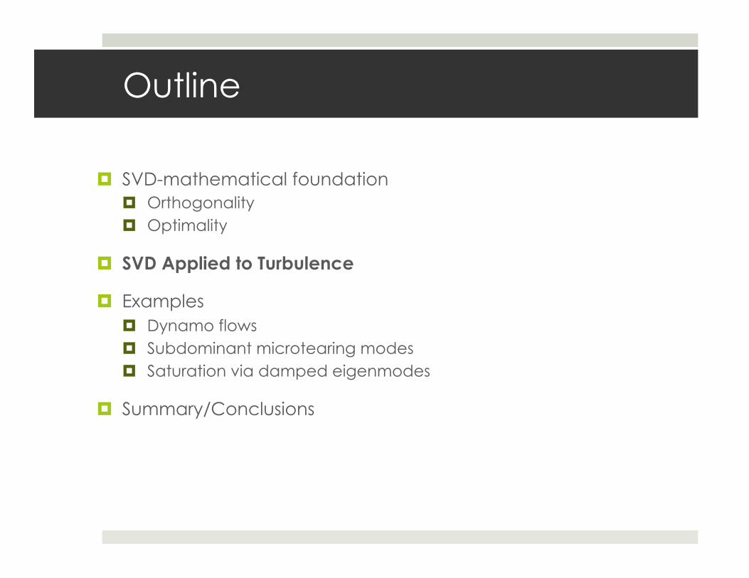
Outline

¤  SVD-mathematical foundation ¤  Orthogonality ¤  Optimality

¤  SVD Applied to turbulence

¤  Examples ¤  Dynamo flows ¤  Subdominant microtearing modes ¤  Saturation via damped eigenmodes

¤  Summary/Conclusions

Singular Value Decomposition

Columns are left singular vectors

Input matrix

Columns are right singular vectors

Diagonal (for upper square portion) containing singular values

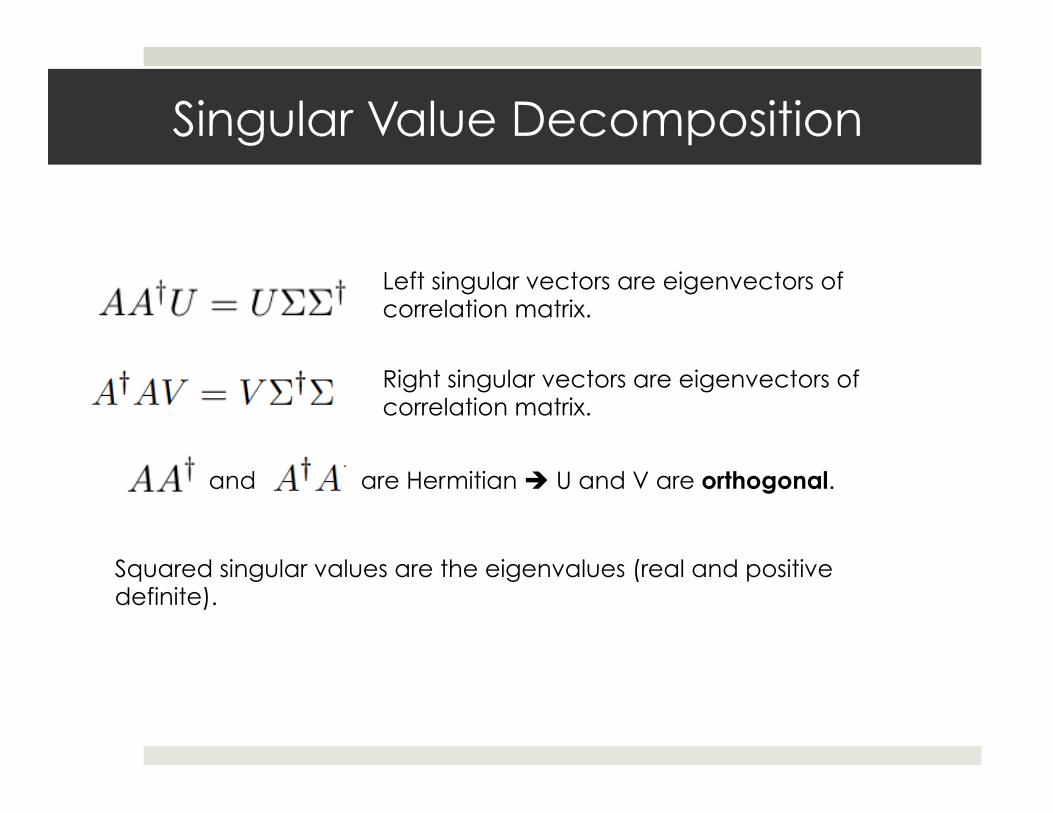
Singular Value Decomposition

Left singular vectors are eigenvectors of correlation matrix.

Right singular vectors are eigenvectors of correlation matrix.

and are Hermitian è U and V are orthogonal.

Squared singular values are the eigenvalues (real and positive definite).

SVD-Optimality

SVD as superposition of rank-1 matrices

SVD produces the best possible rank-r approximation:

SVD is optimal representation:

Minimizes

Outline


¤  SVD Applied to Turbulence



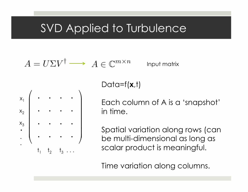
SVD Applied to Turbulence

Input matrix

Data=f(x,t) Each column of A is a ‘snapshot’ in time. Spatial variation along rows (can be multi-dimensional as long as scalar product is meaningful. Time variation along columns.

! ! ! !! ! ! !! ! ! !! ! ! !

"

#

$$$$

%

&

''''

x1

x2

x3 . . .

t1 t2 t3 . . .


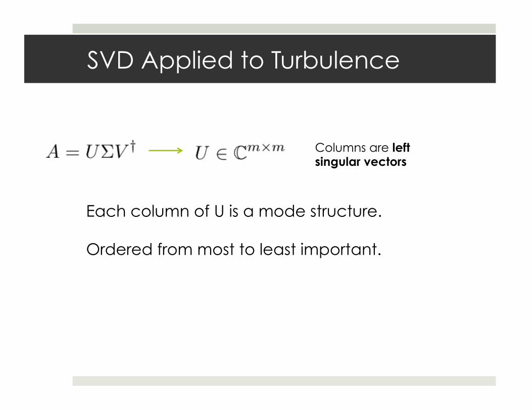
Columns are left singular vectors

Each column of U is a mode structure. Ordered from most to least important.


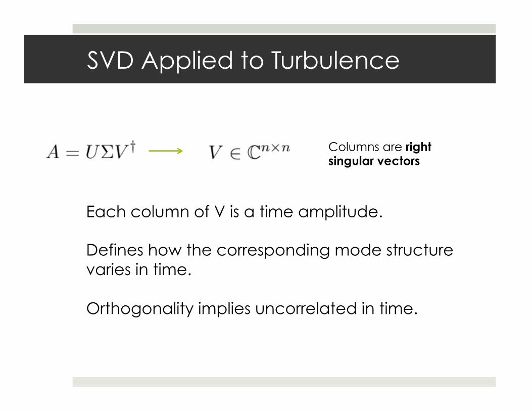
Each column of V is a time amplitude. Defines how the corresponding mode structure varies in time. Orthogonality implies uncorrelated in time.

Columns are right singular vectors


Diagonal (for upper square portion) containing singular values

Squared singular values define how much ‘energy’ (depending on scalar product) is in each mode.

Outline


¤  SVD Applied to Turbulence



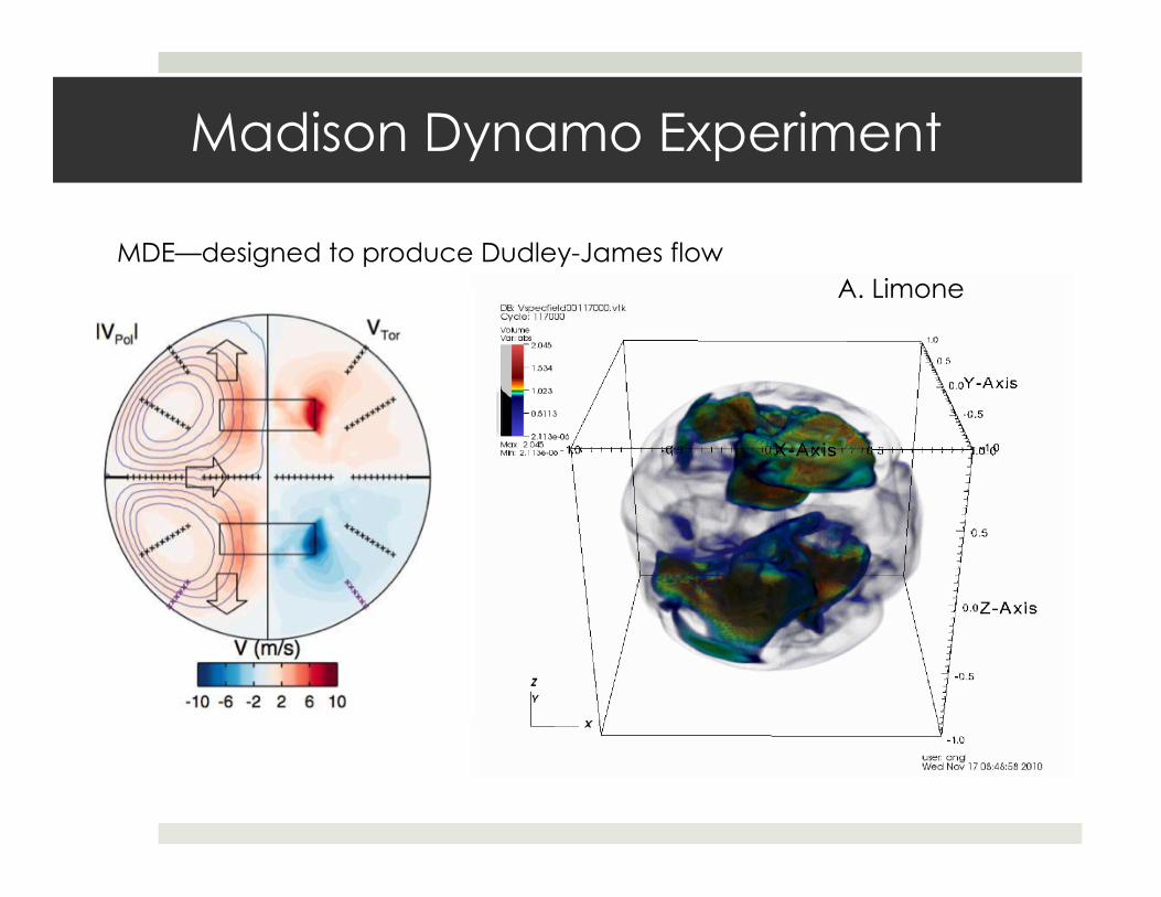
Madison Dynamo Experiment

A. Limone MDE—designed to produce Dudley-James flow

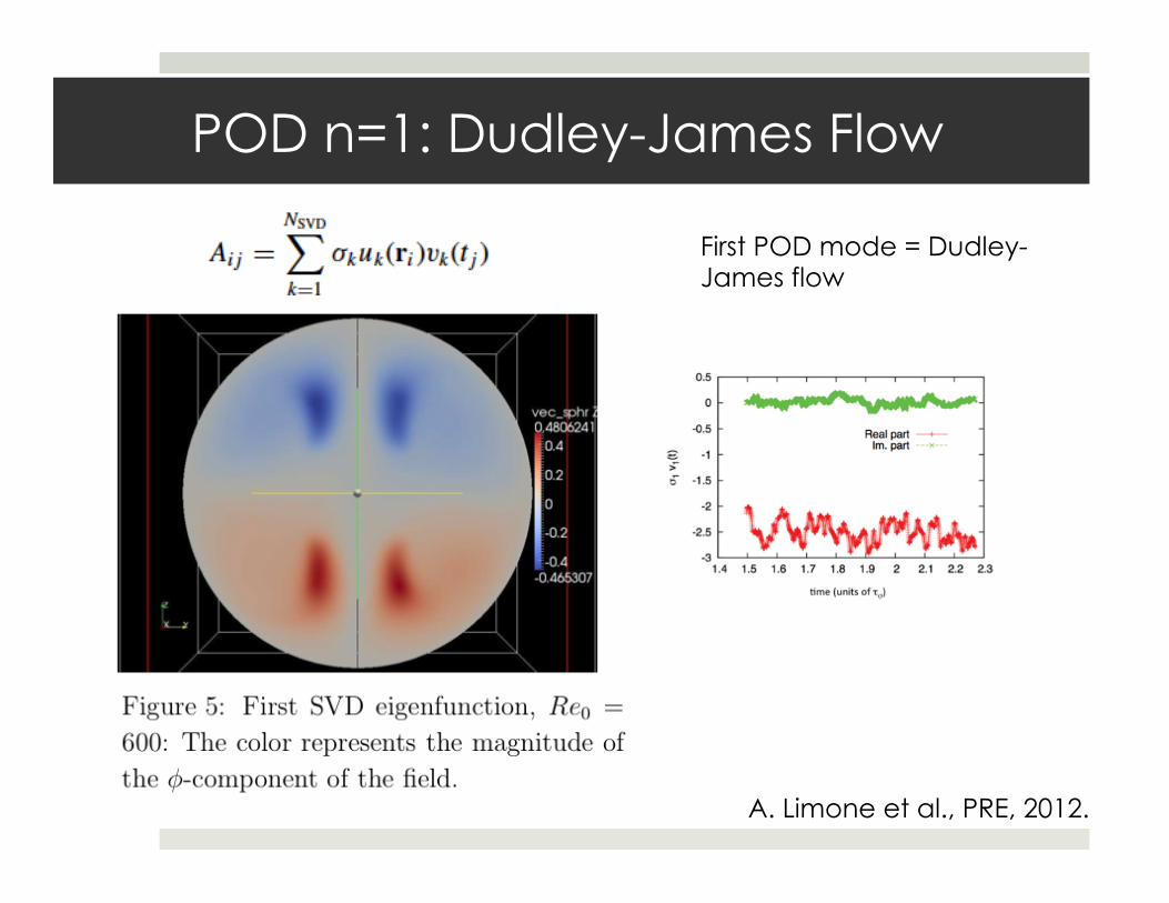
POD n=1: Dudley-James Flow

A. Limone et al., PRE, 2012.

First POD mode = Dudley-James flow

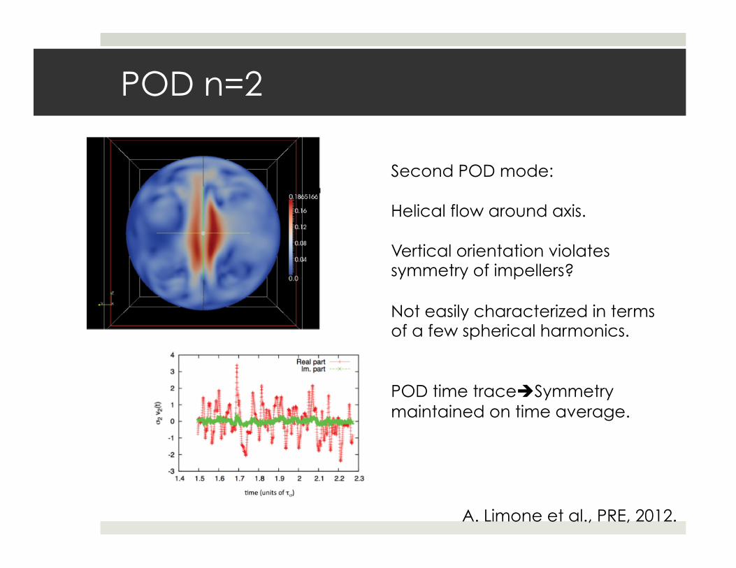
POD n=2


Second POD mode: Helical flow around axis. Vertical orientation violates symmetry of impellers? Not easily characterized in terms of a few spherical harmonics. POD time traceèSymmetry maintained on time average.

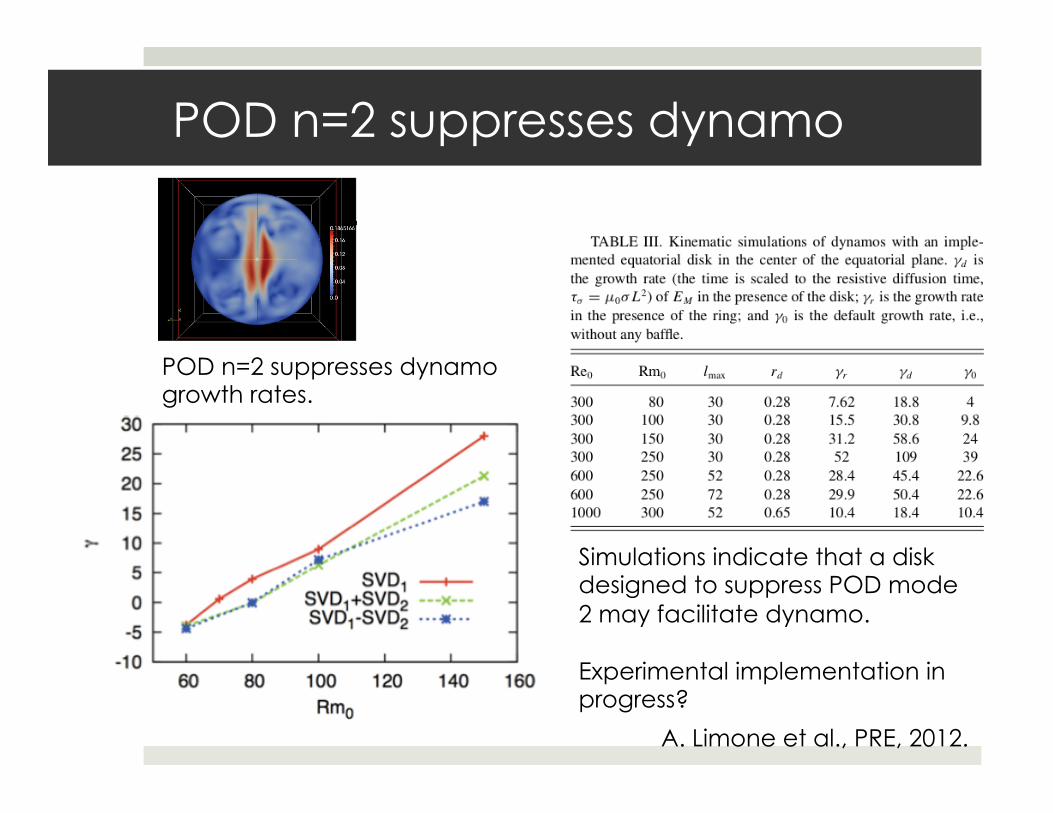
POD n=2 suppresses dynamo


POD n=2 suppresses dynamo growth rates.

Simulations indicate that a disk designed to suppress POD mode 2 may facilitate dynamo. Experimental implementation in progress?

Outline

¤  SVD-mathematical foundation ¤  Orthogonality

¤  Optimality

¤  Examples ¤  Dynamo flows

¤  Subdominant microtearing modes

¤  Saturation via damped eigenmodes


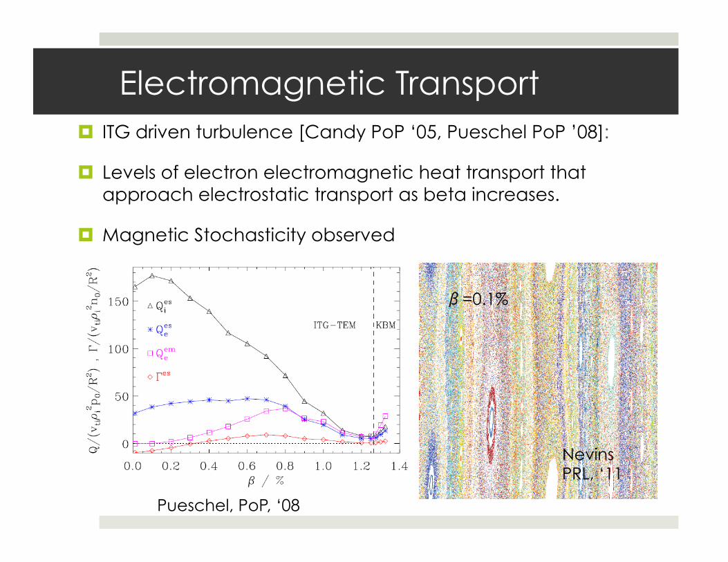
¤  ITG driven turbulence [Candy PoP ‘05, Pueschel PoP ’08]:

¤  Levels of electron electromagnetic heat transport that approach electrostatic transport as beta increases.

¤  Magnetic Stochasticity observed

19

Pueschel, PoP, ‘08

Nevins PRL, ‘11

β=0.1%

Electromagnetic Transport

20

Tearing Parity

z/π z/π

Resonant component extracted by integral along field line. èITG has no resonant component (at kx=0). èTearing parity is resonant.

Ballooning Parity Tearing Parity

What is the cause of stochasticity and EM transport?

21

A|| Mixed Parity in Nonlinear

Simulations: GENE code (gene.rzg.mpg.de)

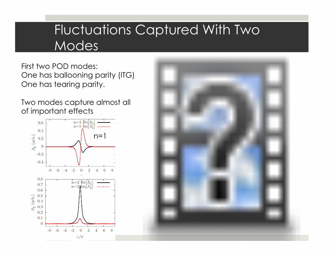
22 Fluctuations Captured With Two Modes

First two POD modes: One has ballooning parity (ITG) One has tearing parity. Two modes capture almost all of important effects

z/π

n=2

n=1

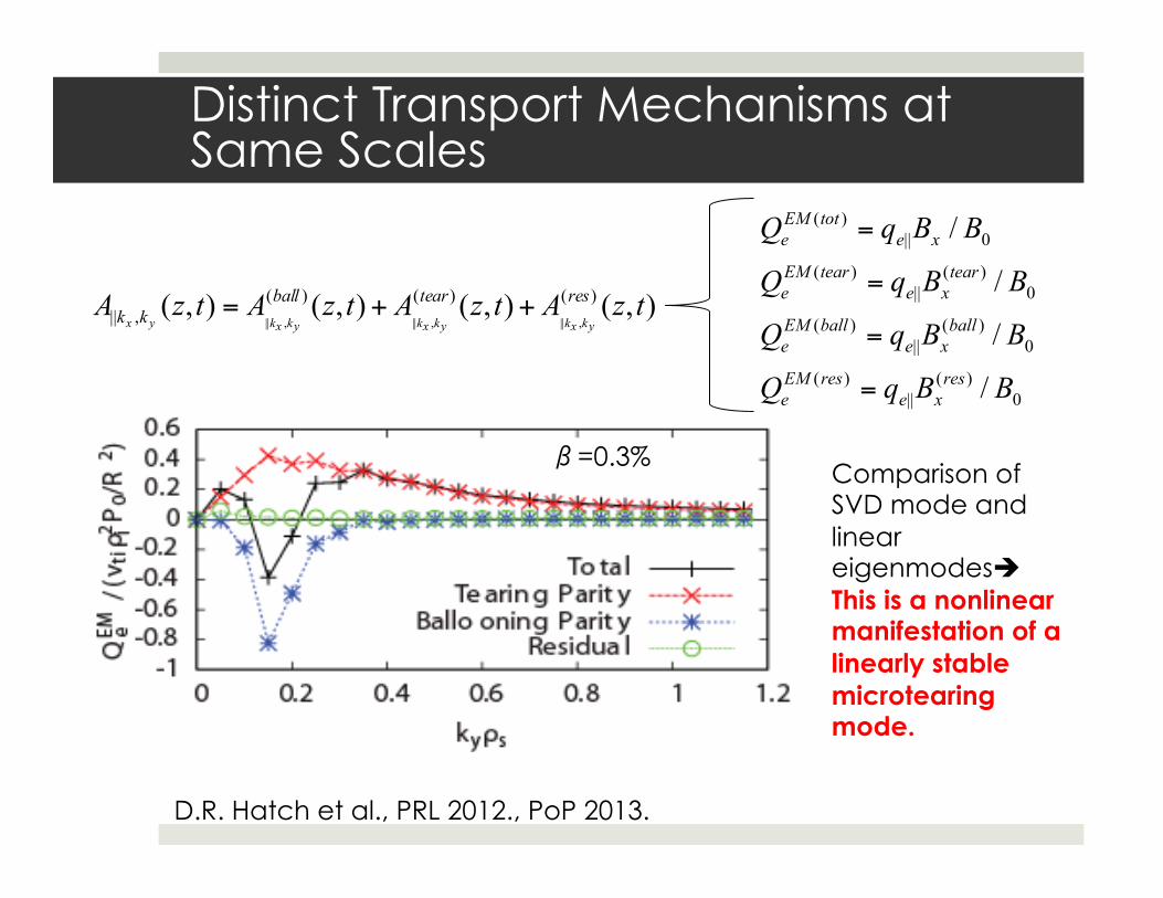
Magnetic transport – superposition of ITG and tearing

0)(

||)(

0)(

||)(

0)(

||)(

0||)(

/

/

/

/

BBqQ

BBqQ

BBqQ

BBqQ

resxe

resEMe

ballxe

ballEMe

tearxe

tearEMe

xetotEM

e

=

=

=

=

),(),(),(),( )()()(,|| ,||,||,||

tzAtzAtzAtzA restearballkk ykxkykxkykxkyx

++=

β=0.3%

23 Distinct Transport Mechanisms at Same Scales

D.R. Hatch et al., PRL 2012., PoP 2013.

Comparison of SVD mode and linear eigenmodesè This is a nonlinear manifestation of a linearly stable microtearing mode.

Outline


¤  Optimality





Gyrokinetics--Energetics

Gyrokinetic free energy equation:

!E!t

=Q+C

Energy source Q proportional to heat flux )

Energy sink C è collisional dissipation (negative definite)

Saturation Through Damped Eigenmodes

there also exist stable eigenmodes that can provide a meansof energy dissipation provided they are driven to finiteamplitude by nonlinear interactions. For each wave vector,numerical discretization allows for N ! nz " nvk " n!degrees of freedom, where the n’s denote the number ofgrid points in each coordinate. The unstable eigenmodedefines only one of these degrees of freedom; the remain-ing degrees of freedom provide an energy sink at largespatial scales.

We seek to characterize the nonlinear state by decom-posing the gyrokinetic distribution function for selectedwave vectors (kx and ky) as a superposition of modes:

gkx;ky#z; vk;!; t$ !X

n

f#n$kx;ky#z; vk;!$h#n$kx;ky

#t$: (1)

The structure f#1$#z; vk;!$ corresponds to the unstable

eigenmode, but its time amplitude h#1$#t$, rather than ex-hibiting its linear behavior e%i#!&i"$t, fluctuates as deter-mined by a balance between the linear drive and thestabilizing influence of nonlinear interactions. The othermodes are also defined by fixed mode structuresf#n$#z; vk;!$ and fluctuate according to their respective

time amplitudes h#n$#t$ in such a way that a superpositionof all the modes exactly reproduces the total distributionfunction at each moment in time. In contrast with theunstable mode, the time amplitudes h#n$#t$ of dampedmodes fluctuate according to a balance between nonlineardrive and linear damping, the latter of which dissipatesenergy from the system, thereby facilitating saturation ofthe turbulence. This decomposition is constructed by per-forming a proper orthogonal decomposition (POD) [7,8]on data from a standard nonlinear gyrokinetic simulation.This provides a means to examine separately the contribu-tion of individual modes, stable or unstable, to the satura-tion of the turbulence.

To study the role of damped modes in saturation, wetrack energy injected into or removed from the turbulenceby using diagnostics related to the conserved (in the ab-sence of drive and dissipation) energylike quantity [9] E !Rdvkd!dzB0#n0T0jgj2=F0 &

RdzD#k?; z$j$j2, where

B0 is the equilibrium magnetic field, $ is the electrostaticpotential, n0 and T0 are the background density andtemperature, respectively, and D is a function of z andthe perpendicular wave numbers. The energy evolvesaccording to

@Ek

@t

!!!!!!!!N:C:! Qk & Ck; (2)

where Q ! Rdvkd!dz#n0T0B0=LT#v2

k &!B0$g'iky !$ is

a term proportional to the heat flux and includes theturbulent drive ( !$ is the gyro-averaged potential, and LT

is the temperature gradient scale length), C representscollisional dissipation, and, in a simulation, whateverartificial dissipation (e.g., hyperdiffusive terms) is included

in the code. The subscript N.C. indicates that this equationdescribes only the nonconservative energy evolution,i.e., processes that inject or dissipate net energy from thefluctuations (as opposed to processes like the E" B non-linearity that move energy from one scale to another in aconservative fashion).The GENE code [10] is used to simulate ITG driven

turbulence defined by the cyclone base case parameters[11] of safety factor q ! 1:4, magnetic shear s ! 0:8,inverse aspect ratio % ! r=R ! 0:18, equilibrium ratiosof density and temperature ni=ne ! Ti=Te ! 1:0, andbackground gradients R=LT ! 6:9 and R=Ln ! 2:2, whereR is the major radius. The perpendicular box size is#Lx; Ly$ ! #126&i; 126&i$, and the number of grid points

is 32" 48" 8 for the #z; vk;!$ coordinates, respectively.The perpendicular spatial resolution consists of 128 gridpoints in the x direction giving kx;max&i ! 3:12 and 64 kyFourier modes for ky;max&i ! 3:15. We deviate from thecyclone base case by using a linearized Landau-Boltzmanncollision operator rather than exclusively artificial dissipa-tion. The collision frequency is '#R=vT$ ! 3:0" 10%3,which is much less than the dynamic time scales of thesystem [e.g., the most unstable mode at ky&i ! 0:3 has agrowth rate "#R=vT$ ! 0:267 and frequency !#R=vT$ !0:783 so that '=!( 10%2]. In these runs, Ck consistsmostly of collisional dissipation but also includes contri-butions from fourth-order hyperdiffusive dissipation in thez and vk coordinates.To illustrate the spatial scale dependence of the energy

balance, we first consider separately the drive term Qk andthe dissipation term Ck in Eq. (2). Figure 1 shows Qk andCk from the saturated state of a simulation, averaged overthe parallel coordinate and time. In Fig. 1(a), kx depen-dence is shown and ky is summed; in Fig. 1(b), ky depen-dence is shown and kx is summed. There is a significantamount of dissipation at all scales, including ky ! 0:0 andhigh k?. However, the largest range of peak dissipationcorresponds with the same scales where the energy drivepeaks. As described in detail below, the drive Qk is

FIG. 1 (color online). Energy drive Qk and dissipation Ck timeaveraged over the nonlinear state and averaged over the zdirection, as a function of (a) kx summed over ky and (b) kysummed over kx.

PRL 106, 115003 (2011) P HY S I CA L R EV I EW LE T T E R Sweek ending

18 MARCH 2011

115003-2

--Cyclone Base Case ITG (and everything else we’ve looked at): Significant dissipation in region of instability (Hatch et al. PRL 2011). --Damped modes nonlinearly driven at same scales as ITG èWhat modes are responsible?

!E!t

=Q+CEnergy source Q proportional to heat flux

Energy sink C è collisional dissipation

Damped Eigenmodes in Simple System

¤  Goal: examine simple system in order to identify damped eigenmodes ¤  Slab ITG

¤  Adiabatic electrons

¤  Integrated over perpendicular velocity

¤  Model similar to Watanabe, Sugama PoP ’04 (but we keep range of kz)

¤  Examine three levels ¤  Linear spectra

¤  Pseudospectra—bridge between linear and nonlinear

¤  Nonlinear--SVD

DNA Code

DNA code: Direct Numerical Analysis of Fundamental Gyrokinetic Turbulence Dynamics Fully Spectral: Fourier in three spatial dimensions Hermite in parallel velocity Developed from scratch, but much of the structure and many algorithms inspired and informed by GENE.

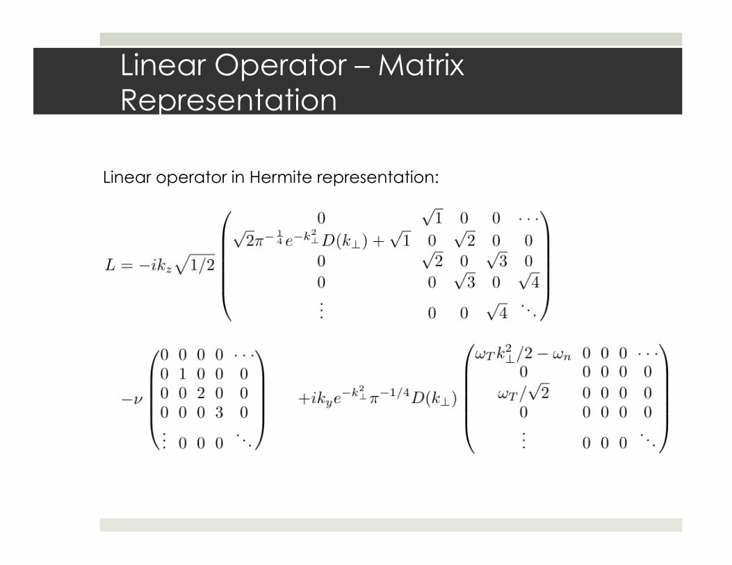
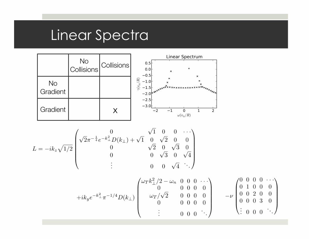
Linear Operator – Matrix Representation

Linear operator in Hermite representation:

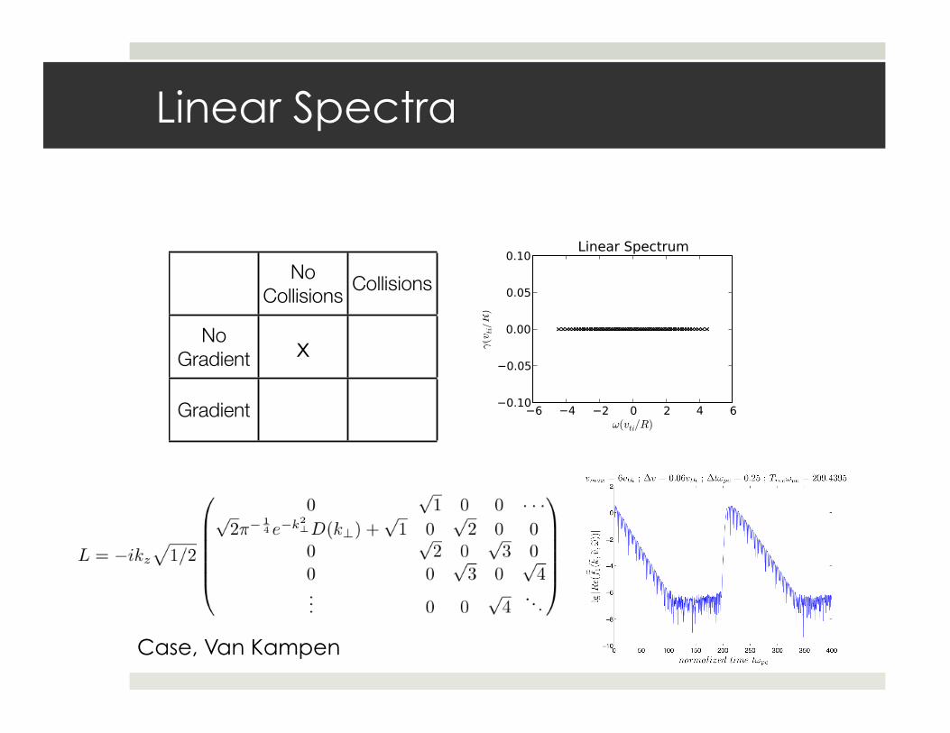
Linear Spectra

No Collisions

Collisions

No Gradient x

Gradient

Case, Van Kampen

Linear Spectra

No Collisions

Collisions

No Gradient x

Gradient

(Skiff et al. PRL ’98, Ng et al. PRL ’99)

Linear Spectra

No Collisions

Collisions

No Gradient

Gradient x

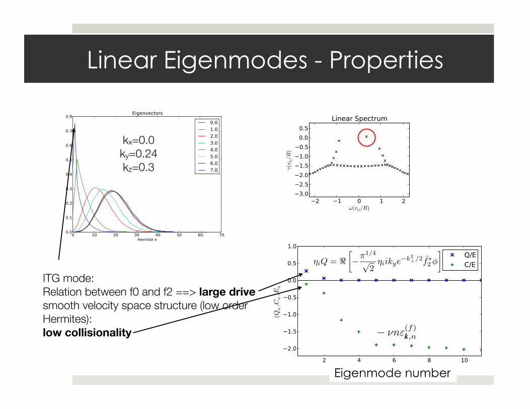
Linear Eigenmodes - Properties

kx=0.0ky=0.24kz=0.3

ITG mode: Relation between f0 and f2 ==> large drivesmooth velocity space structure (low order Hermites):low collisionality

4

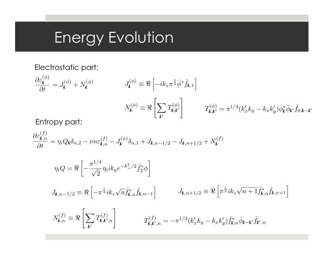
The entropy evolution equation is

∂ε(f)k,n

∂t= ηiQkδn,2 − νnε(f)k,n − J (φ)

k δn,1 + Jk,n−1/2 − Jk,n+1/2 +N (f)k . (25)

The energy drive term acts only on the second order Hermite polynomial and is proportional to the heat flux,

ηiQ = ��−π1/4

√2ηiikye

−k2⊥/2f∗

2φ

�, (26)

The second term on the RHS represents collisional dissipation, the phase mixing terms are defined as

Jk,n−1/2 ≡ ��−π

12 ikz

√nf∗

k,nfk,n−1

�, (27)

and

Jk,n+1/2 ≡ ��π

12 ikz

√n+ 1f∗

k,nfk,n+1

�, (28)

and the nonlinear transfer term is,

N (f)k,n ≡ �

��

k�T (f)

k,k’,n

�, (29)

where the nonlinear entropy transfer function is defined as

T (f)k,k�,n = −π1/2(k�xky − kxk

�y)f

∗k,nφk−k� fk�,n. (30)

Discuss conservation.

A. Second subsection

IV. LANDAU DAMPING IN THE PRESENCE OF NONLINEARITY

γL ≡J (φ)

k − Jk,1/2

2εk,0(31)

ωnl ∼ kzvTi (32)

ωnl ∼ kyvTiρi/Ln (33)

ωnl�φ(t)∗φ(t+ τ)dt

γlinγL,lin

γL,nl

kzvTi

4


∂ε(f)k,n


k δn,1 + Jk,n−1/2 − Jk,n+1/2 +N (f)k . (25)


ηiQ = ��−π1/4

√2ηiikye

−k2⊥/2f∗

2φ

�, (26)


Jk,n−1/2 ≡ ��−π

12 ikz

√nf∗

k,nfk,n−1

�, (27)

and

Jk,n+1/2 ≡ ��π

12 ikz

√n+ 1f∗

k,nfk,n+1

�, (28)


N (f)k,n ≡ �

��

k�T (f)

k,k’,n

�, (29)



�y)f

∗k,nφk−k� fk�,n. (30)




γL ≡J (φ)

k − Jk,1/2

2εk,0(31)

ωnl ∼ kzvTi (32)



γlinγL,lin

γL,nl

kzvTi

Eigenmode number Eigenmode number


kx=0.0ky=0.24kz=0.3

Drift Wave:Relation between f0 and f2 ==> moderate drivesmooth velocity space structure (low order Hermites):low collisionality

4


∂ε(f)k,n


k δn,1 + Jk,n−1/2 − Jk,n+1/2 +N (f)k . (25)


ηiQ = ��−π1/4

√2ηiikye

−k2⊥/2f∗

2φ

�, (26)


Jk,n−1/2 ≡ ��−π

12 ikz

√nf∗

k,nfk,n−1

�, (27)

and

Jk,n+1/2 ≡ ��π

12 ikz

√n+ 1f∗

k,nfk,n+1

�, (28)


N (f)k,n ≡ �

��

k�T (f)

k,k’,n

�, (29)



�y)f

∗k,nφk−k� fk�,n. (30)




γL ≡J (φ)

k − Jk,1/2

2εk,0(31)

ωnl ∼ kzvTi (32)



γlinγL,lin

γL,nl

kzvTi

4


∂ε(f)k,n


k δn,1 + Jk,n−1/2 − Jk,n+1/2 +N (f)k . (25)


ηiQ = ��−π1/4

√2ηiikye

−k2⊥/2f∗

2φ

�, (26)


Jk,n−1/2 ≡ ��−π

12 ikz

√nf∗

k,nfk,n−1

�, (27)

and

Jk,n+1/2 ≡ ��π

12 ikz

√n+ 1f∗

k,nfk,n+1

�, (28)


N (f)k,n ≡ �

��

k�T (f)

k,k’,n

�, (29)



�y)f

∗k,nφk−k� fk�,n. (30)




γL ≡J (φ)

k − Jk,1/2

2εk,0(31)

ωnl ∼ kzvTi (32)



γlinγL,lin

γL,nl

kzvTi

Eigenmode number


kx=0.0ky=0.24kz=0.3

Landau roots:Relation between f0 and f2 ==> virtually 0smooth velocity space structure (low order Hermites):high collisionality

4


∂ε(f)k,n


k δn,1 + Jk,n−1/2 − Jk,n+1/2 +N (f)k . (25)


ηiQ = ��−π1/4

√2ηiikye

−k2⊥/2f∗

2φ

�, (26)


Jk,n−1/2 ≡ ��−π

12 ikz

√nf∗

k,nfk,n−1

�, (27)

and

Jk,n+1/2 ≡ ��π

12 ikz

√n+ 1f∗

k,nfk,n+1

�, (28)


N (f)k,n ≡ �

��

k�T (f)

k,k’,n

�, (29)



�y)f

∗k,nφk−k� fk�,n. (30)




γL ≡J (φ)

k − Jk,1/2

2εk,0(31)

ωnl ∼ kzvTi (32)



γlinγL,lin

γL,nl

kzvTi

4


∂ε(f)k,n


k δn,1 + Jk,n−1/2 − Jk,n+1/2 +N (f)k . (25)


ηiQ = ��−π1/4

√2ηiikye

−k2⊥/2f∗

2φ

�, (26)


Jk,n−1/2 ≡ ��−π

12 ikz

√nf∗

k,nfk,n−1

�, (27)

and

Jk,n+1/2 ≡ ��π

12 ikz

√n+ 1f∗

k,nfk,n+1

�, (28)


N (f)k,n ≡ �

��

k�T (f)

k,k’,n

�, (29)



�y)f

∗k,nφk−k� fk�,n. (30)




γL ≡J (φ)

k − Jk,1/2

2εk,0(31)

ωnl ∼ kzvTi (32)



γlinγL,lin

γL,nl

kzvTi

Eigenmode number

Pseudospectrum – Slab ITG

ITG (and to a lesser degree ISW):Closely nested contours

Closely nested surfaces around ITG mode (and to a lesser extent around DW.

Trefethen-Science, New Series, Vol. 261, No. 5121. (Jul. 30, 1993), pp. 578-584.Trefethen-SIAM REV. Vol. 39, No. 3, pp. 383–406, September 1997

“. . . even if all of the eigenvalues of a linear system are distinct and lie well inside the lower half plane, inputs to

that system may be amplified by arbitrarily large factors if the eigenfunctions are not orthogonal to one another.”

Classic Example:

Pseudospectra—Trefethen, SIAM review, 1997.

Pseudospectrum – Slab ITG

Highly non-orthogonal in this region

All frequencies in this region are highly resonant

Would not expect fluctuations to match eigenvalues here.




Classic Example:

Direct Eigenmode Decompostion Infeasible

•Case-Van Kampen emphasized that eigenmodes form complete basis (even though they are nonorthogonal)

•Eigenvectors of adjoint operator serve as projection operators

•In practice nonorthogonality is too extreme==>cannot associate any quadratic quantity (e.g. free energy or heat flux) uniquely with individual eigenmodes.

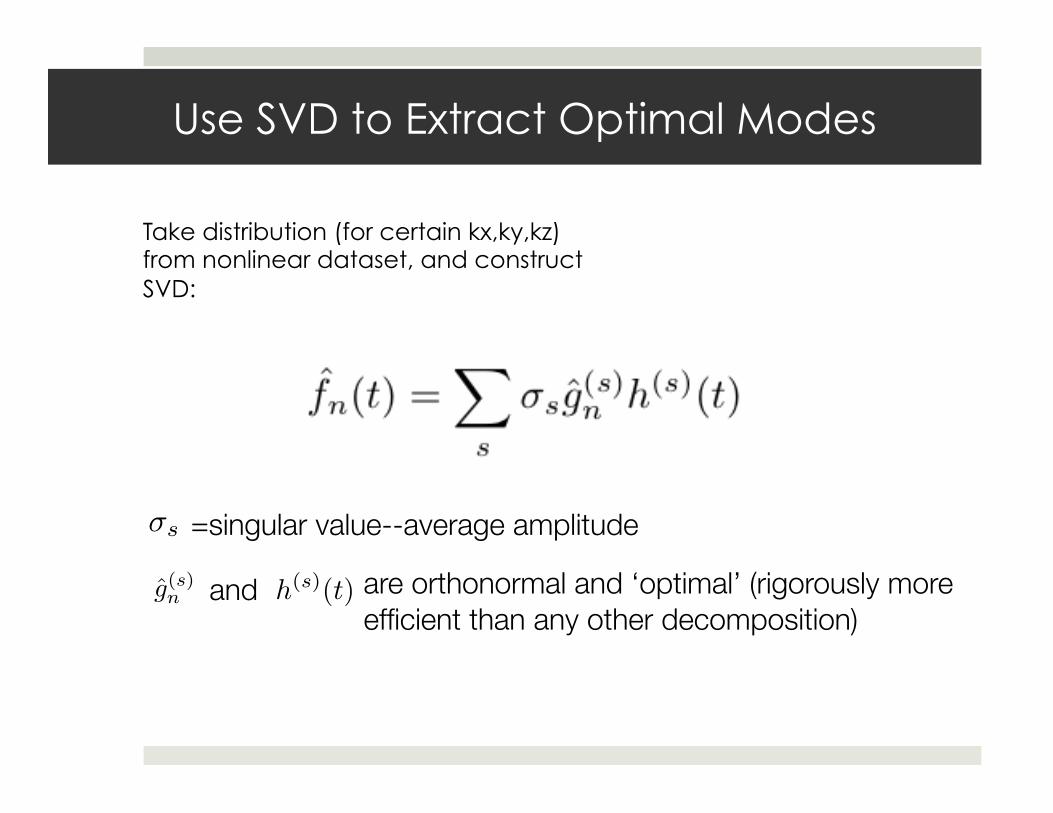
Use SVD to Extract Optimal Modes

Take distribution (for certain kx,ky,kz) from nonlinear dataset, and construct SVD:

4

Jn−1/2 = −1

2π

12 ikz

√nf∗

nfn−1 (50)

Jn+1/2 = −1

2π

12 ikz

√n+ 1f∗

nfn+1 (51)

The free energy equation [? ] for this system can be derivedfor the gyrokinetic equations by operating with,

ε[X] ≡ Re

�� ∞

−∞

�f

F0+ e−k2

⊥/2φ

�∗Xdv

�. (52)

This can be applied in the Hermite representation by notingthat,

� ∞

−∞

�f

F0+ e−k2

⊥/2φ

�∗hdv =

�

n

�π1/2fn + π1/4e−k2

⊥/2φδn,0�∗

hn, (53)

where h is any function with a Hermite expansion of the formof Eq. ??. Operating on the distribution function produces thefree energy,

εn = ε(f)n + ε(φ)δn,0, (54)

where the entropy part is defined as,

ε(f)n ≡ 1

2π

12 |fn|2, (55)

and the electrostatic part is,

ε(φ)/ε(f)0 = π−14 e−k2

⊥D(k⊥). (56)

E =1

2

�

n

��fn��2π1/2 +

1

2D(k2⊥) |φ|

2 , (57)

where D(k2⊥) = 1τ+1−Γ0(b)

. The energy evolution equationis produced by operating on each term on the RHS of Eq. 38as will be outlined below. By summing over all k, one canextract the non-vanishing terms which define the sources andsinks of the system.

The density gradient, ωn, term in the energy equation isproportional to iky g0φ. Since g0 is proportional to φ, this termdrops out when summed over k due to the reality constraint.

The temperature gradient term produces the energy drive,

ωTQ = −π1/4

√2ωT ikye

−k2⊥/2f∗

2φ. (58)

The parallel electric field has two terms–one proportionalto ikz|φ|2 which vanishes when summed over k and anotherterm,

−π1/4ikz f∗1 e

−k2⊥/2φ, (59)

which will be shown to cancel with quantities in the phase-mixing term.

The phase mixing term produces two results,−ikzπ1/4e−k2

⊥/2φ∗f1, which cancels with the term inexpression 59, and additional terms,

�

n

π1/2(−ikz)�√

nf∗nfn−1 +

√n+ 1f∗

nfn+1

�, (60)

which cancel in the sum over n. This cancellation can be seen,e.g., by considering the expressions in 60 for n = m− 1 andn = m. The

√n+ 1g∗ngn+1 term for n = m − 1 cancels

exactly with the g∗ngn−1 term for n = m. In other words, thephase-mixing term transfers energy in a conservative linearcascade through velocity space. Numerically this is violatedonly at n = nmax where the Hermite representation is trun-cated and thus well-behaved energetics is only expected withsufficient velocity space resolution.

Finally, the collision term provides the energy sink of thesystem,

C = −π1/2�

n

νn��fn

��2. (61)

The final energy equation is,

∂E

∂t=

�

k

[π1/4

√2ωT ikye

−k2⊥/2f∗

2φ− π1/2�

n

νn��fn

��2].

(62)

A. Nonlinear Energy Transfer

Fill in some explanation:

Tn,k,k� = −π1/2(k�xky − kxk�y)f

∗n,kφk−k� fn,k� (63)

Tφ,k,k� = π1/4(k�xky − kxk�y)φ

∗kφk� f0,k−k� (64)

fn(t) =�

s

σsg(s)n h(s)(t) (65)

σs (66)

g(s)n (67)

h(s)(t) (68)

||Agn − zgn|| (69)

4

Jn−1/2 = −1

2π

12 ikz

√nf∗

nfn−1 (50)

Jn+1/2 = −1

2π

12 ikz

√n+ 1f∗

nfn+1 (51)


ε[X] ≡ Re

�� ∞

−∞

�f

F0+ e−k2

⊥/2φ

�∗Xdv

�. (52)


� ∞

−∞

�f

F0+ e−k2

⊥/2φ

�∗hdv =

�

n

�π1/2fn + π1/4e−k2

⊥/2φδn,0�∗

hn, (53)


εn = ε(f)n + ε(φ)δn,0, (54)


ε(f)n ≡ 1

2π

12 |fn|2, (55)


ε(φ)/ε(f)0 = π−14 e−k2

⊥D(k⊥). (56)

E =1

2

�

n

��fn��2π1/2 +

1

2D(k2⊥) |φ|

2 , (57)





ωTQ = −π1/4

√2ωT ikye

−k2⊥/2f∗

2φ. (58)


−π1/4ikz f∗1 e

−k2⊥/2φ, (59)




�

n

π1/2(−ikz)�√

nf∗nfn−1 +

√n+ 1f∗

nfn+1

�, (60)





C = −π1/2�

n

νn��fn

��2. (61)


∂E

∂t=

�

k

[π1/4

√2ωT ikye

−k2⊥/2f∗

2φ− π1/2�

n

νn��fn

��2].

(62)






∗kφk� f0,k−k� (64)

fn(t) =�

s


σs (66)

g(s)n (67)

h(s)(t) (68)

||Agn − zgn|| (69)

4

Jn−1/2 = −1

2π

12 ikz

√nf∗

nfn−1 (50)

Jn+1/2 = −1

2π

12 ikz

√n+ 1f∗

nfn+1 (51)


ε[X] ≡ Re

�� ∞

−∞

�f

F0+ e−k2

⊥/2φ

�∗Xdv

�. (52)


� ∞

−∞

�f

F0+ e−k2

⊥/2φ

�∗hdv =

�

n

�π1/2fn + π1/4e−k2

⊥/2φδn,0�∗

hn, (53)


εn = ε(f)n + ε(φ)δn,0, (54)


ε(f)n ≡ 1

2π

12 |fn|2, (55)


ε(φ)/ε(f)0 = π−14 e−k2

⊥D(k⊥). (56)

E =1

2

�

n

��fn��2π1/2 +

1

2D(k2⊥) |φ|

2 , (57)





ωTQ = −π1/4

√2ωT ikye

−k2⊥/2f∗

2φ. (58)


−π1/4ikz f∗1 e

−k2⊥/2φ, (59)




�

n

π1/2(−ikz)�√

nf∗nfn−1 +

√n+ 1f∗

nfn+1

�, (60)





C = −π1/2�

n

νn��fn

��2. (61)


∂E

∂t=

�

k

[π1/4

√2ωT ikye

−k2⊥/2f∗

2φ− π1/2�

n

νn��fn

��2].

(62)






∗kφk� f0,k−k� (64)

fn(t) =�

s


σs (66)

g(s)n (67)

h(s)(t) (68)

||Agn − zgn|| (69)

=singular value--average amplitude

and are orthonormal and ‘optimal’ (rigorously more efficient than any other decomposition)

Already Noted: direct projection onto linear eigenmodes is meaningless Go backwards from SVD: Get ‘pseudo-eigenvalues’ by minimizing over the complex plane for a given SVD mode gn This is zero for an exact eigenvector pseudo-eigenvalue is the location in the complex plane where is minimized

Pseudo-eigenvalues From SVD Modes

Nonlinear spectra

•Typically one mode near ITG•One near ISW•One or more with negative Q•Typically 3-5 modes contribute to energy balance.•Landau-like roots not a significant player

Combine information -linear -pseudospectra -nonlinear

Mode growth/damping rates for Q and C

Net damping rate (including amplitude)

How close to being an eigenvalue

Nonlinear spectra


ITG DW

ITG and DW clearly identified.

ITG and DW clearly identified.

Nonlinear spectra


Typically one or more modes with negative Q—i.e., inward heat flux. Significant energy sink. Dissimilar to anything in the linear spectrum. Landau-like roots don’t play big role (at low k).

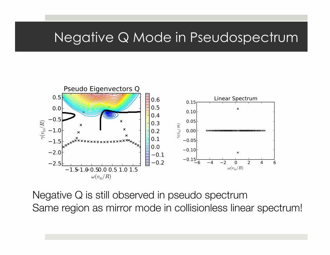
Negative Q Mode in Pseudospectrum

Negative Q is still observed in pseudo spectrumSame region as mirror mode in collisionless linear spectrum!

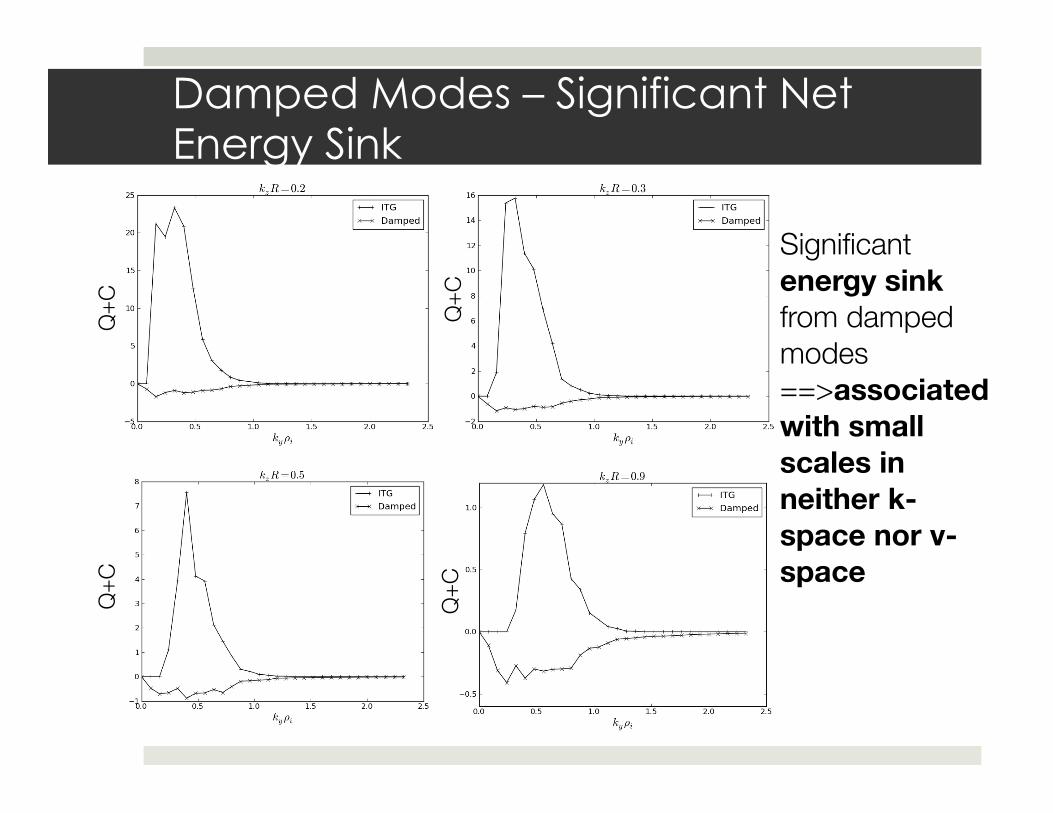
Damped Modes – Significant Net Energy Sink

Q+

C

Q+

C

Q+

C

Q+

C

Significant energy sink from damped modes==>associated with small scales in neither k-space nor v-space

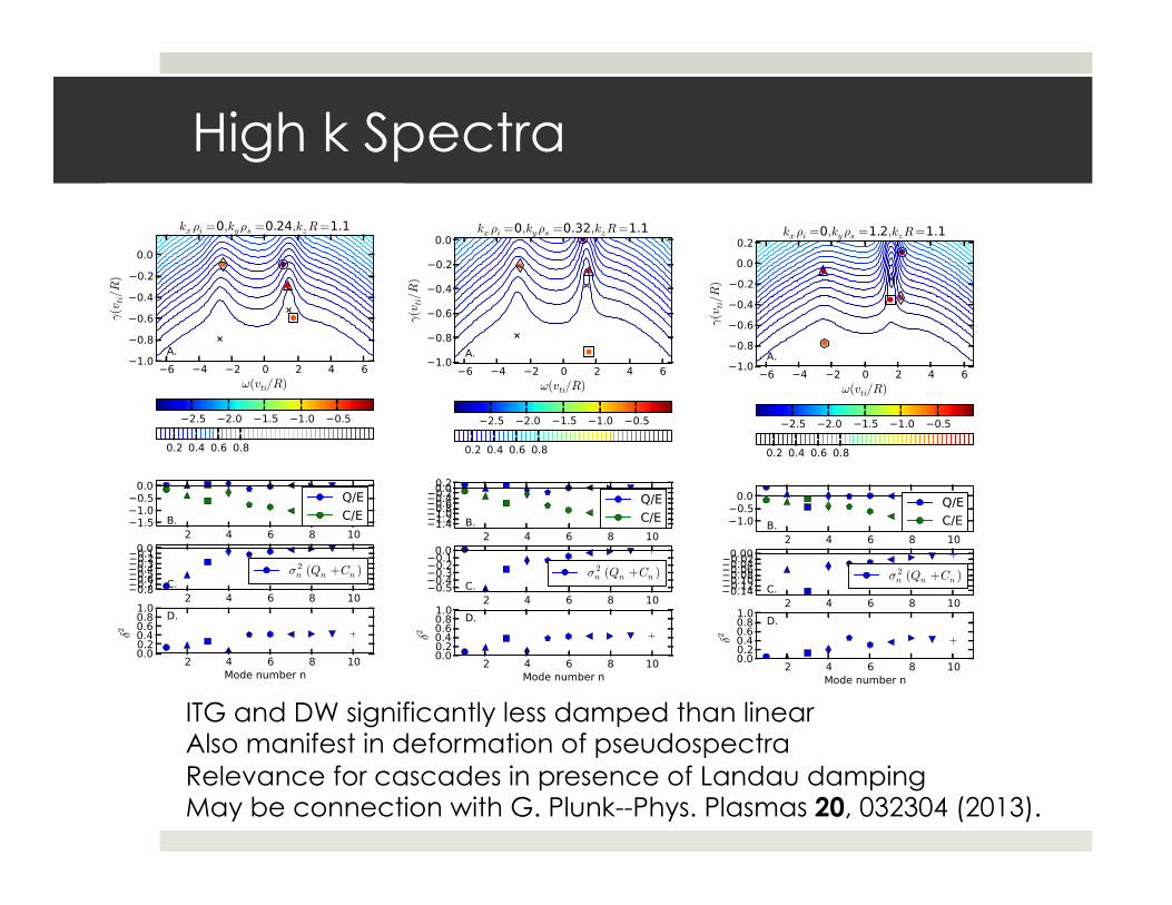
High k Spectra

•Ion sound wave and ITG are significantly less damped (sometimes destabilized)

•Damping rate does not match Landau damping rate.

•Also manifest in deformation of pseudospectra

ITG and DW significantly less damped than linear Also manifest in deformation of pseudospectra Relevance for cascades in presence of Landau damping May be connection with G. Plunk--Phys. Plasmas 20, 032304 (2013).

Outline


¤  Optimality





Summary Conclusions

¤  POD/SVD extracts optimal, orthogonal representation of turbulence fluctuations

¤  Examples ¤  Dynamo—SVD identifies mode that suppresses dynamo ¤  Electromagnetic gyrokinetic ITG simulations

¤  Linearly stable microtearing mode responsible for magnetic stochasticity and transport

¤  Damped eigenmodes—damped eigenmodes provide potent energy sink in region of energy drive. ¤  Marginally stable drift wave and mode with negative Q

identified in nonlinear spectrum ¤  Negative Q mode absent from linear spectrum, but can

be identified in pseudospectrum

References

¤  POD/SVD: ¤  Berkooz, et al. Annu. Rev. Fluid. Mech., 1993.

¤  Holmes et al., (1996) ‘Turbulence, Coherent Structures, Dynamical Systems and Symmetry’, New York: Cambridge University Press

¤  Dynamo+POD ¤  Limone et al., PRE, 2013

¤  Electromagnetic gyrokinetic simulations and subdominant microtearing modes ¤  Hatch et al., PRL, 2012, Hatch et al., PoP, 2013

¤  Damped eigenmodes as saturation mechanism ¤  Fluid models: Terry et al., PoP, 2006

¤  Gyrokinetics: Hatch et al. PRL 2011, PoP, 2012

¤  Higher Order Singular Value Decomposition (HOSVD)—high-dimensional generalization of SVD ¤  Hatch et al., JCP, 2012

¤  Other recent plasma applications ¤  Futatani et al., PoP, 2009

¤  del-Castillo Negrete et al., JCP 2007, PoP 2008

Pseudospectra




Classic Example:

Hermite representation in GK

èHermite polynomials—natural representation of parallel velocity in GK

Higher order singular value decomposition (HOSVD) applied to 6D gyrokinetics (5D plus time)—extracts mode structures for each coordinate.

Hatch et al. JCP ‘12

Energy Evolution

3

D(k⊥) ≡1 + δky,0δkz,0∆/(1− Γ0(k2x))

τ + 1− Γ0(k2⊥)(13)

φ = π14 e−k2

⊥/2D(k⊥)f0 (14)

The heat flux Q ≡ �p∂yφ� becomes

Q = −π1/4

√2

�

kx,ky,kz

ikyφf∗2 . (15)

For derivations of Eqs. (xxx) see Appendix B.

III. FREE ENERGY CONSERVATION AND EVOLUTION

The nonlinearly conserved free energy equation [? ] for this system can be derived by operating on Eq. ?? with,

εn[Xn] ≡ Re��

π12 fn + π

14 φδn,0

�∗Xn

�. (16)

The free energy is,

εk,n = ε(f)k,n + ε(φ)k δn,0, (17)


ε(f)k,n ≡ 1

2π

12 |fk,n|2, (18)


ε(φ)k ≡ 1

2D(k⊥)|φk|2 (19)

ε(φ)k /ε(f)k,0 = e−k2⊥D(k⊥). (20)

The k- and n-resolved free energy evolution equation is produced by operating on the RHS of Eq. ??, and produces equations

for both the electrostatic and entropy parts of the free energy. The evolution equation for the electrostatic free energy is

∂ε(φ)k∂t

= J (φ)k +N (φ)

k , (21)

where

J (φ)k ≡ �

�−ikzπ

14 φ∗fk,1

�, (22)

and

N (φ)k ≡ �

��

k�T (φ)

k,k’

�, (23)

with the nonlinear transfer function for the electrostatic energy defined as,

T (φ)k,k’ = π1/4(k�xky − kxk

�y)φ

∗k φk� f0,k−k� . (24)

3

D(k⊥) ≡1 + δky,0δkz,0∆/(1− Γ0(k2x))

τ + 1− Γ0(k2⊥)(13)

φ = π14 e−k2

⊥/2D(k⊥)f0 (14)


Q = −π1/4

√2

�

kx,ky,kz

ikyφf∗2 . (15)





π12 fn + π

14 φδn,0

�∗Xn

�. (16)

The free energy is,

εk,n = ε(f)k,n + ε(φ)k δn,0, (17)


ε(f)k,n ≡ 1

2π

12 |fk,n|2, (18)


ε(φ)k ≡ 1

2D(k⊥)|φk|2 (19)

ε(φ)k /ε(f)k,0 = e−k2⊥D(k⊥). (20)



∂ε(φ)k∂t

= J (φ)k +N (φ)

k , (21)

where

J (φ)k ≡ �

�−ikzπ

14 φ∗fk,1

�, (22)

and

N (φ)k ≡ �

��

k�T (φ)

k,k’

�, (23)



�y)φ

∗k φk� f0,k−k� . (24)

3

D(k⊥) ≡1 + δky,0δkz,0∆/(1− Γ0(k2x))

τ + 1− Γ0(k2⊥)(13)

φ = π14 e−k2

⊥/2D(k⊥)f0 (14)


Q = −π1/4

√2

�

kx,ky,kz

ikyφf∗2 . (15)





π12 fn + π

14 φδn,0

�∗Xn

�. (16)

The free energy is,

εk,n = ε(f)k,n + ε(φ)k δn,0, (17)


ε(f)k,n ≡ 1

2π

12 |fk,n|2, (18)


ε(φ)k ≡ 1

2D(k⊥)|φk|2 (19)

ε(φ)k /ε(f)k,0 = e−k2⊥D(k⊥). (20)



∂ε(φ)k∂t

= J (φ)k +N (φ)

k , (21)

where

J (φ)k ≡ �

�−ikzπ

14 φ∗fk,1

�, (22)

and

N (φ)k ≡ �

��

k�T (φ)

k,k’

�, (23)



�y)φ

∗k φk� f0,k−k� . (24)

3

D(k⊥) ≡1 + δky,0δkz,0∆/(1− Γ0(k2x))

τ + 1− Γ0(k2⊥)(13)

φ = π14 e−k2

⊥/2D(k⊥)f0 (14)


Q = −π1/4

√2

�

kx,ky,kz

ikyφf∗2 . (15)





π12 fn + π

14 φδn,0

�∗Xn

�. (16)

The free energy is,

εk,n = ε(f)k,n + ε(φ)k δn,0, (17)


ε(f)k,n ≡ 1

2π

12 |fk,n|2, (18)


ε(φ)k ≡ 1

2D(k⊥)|φk|2 (19)

ε(φ)k /ε(f)k,0 = e−k2⊥D(k⊥). (20)



∂ε(φ)k∂t

= J (φ)k +N (φ)

k , (21)

where

J (φ)k ≡ �

�−ikzπ

14 φ∗fk,1

�, (22)

and

N (φ)k ≡ �

��

k�T (φ)

k,k’

�, (23)



�y)φ

∗k φk� f0,k−k� . (24)

4


∂ε(f)k,n


k δn,1 + Jk,n−1/2 − Jk,n+1/2 +N (f)k . (25)


ηiQ = ��−π1/4

√2ηiikye

−k2⊥/2f∗

2φ

�, (26)


Jk,n−1/2 ≡ ��−π

12 ikz

√nf∗

k,nfk,n−1

�, (27)

and

Jk,n+1/2 ≡ ��π

12 ikz

√n+ 1f∗

k,nfk,n+1

�, (28)


N (f)k,n ≡ �

��

k�T (f)

k,k’,n

�, (29)



�y)f

∗k,nφk−k� fk�,n. (30)




γL ≡J (φ)

k − Jk,1/2

2εk,0(31)

ωnl ∼ kzvTi (32)



γlinγL,lin

γL,nl

kzvTi

4


∂ε(f)k,n


k δn,1 + Jk,n−1/2 − Jk,n+1/2 +N (f)k . (25)


ηiQ = ��−π1/4

√2ηiikye

−k2⊥/2f∗

2φ

�, (26)


Jk,n−1/2 ≡ ��−π

12 ikz

√nf∗

k,nfk,n−1

�, (27)

and

Jk,n+1/2 ≡ ��π

12 ikz

√n+ 1f∗

k,nfk,n+1

�, (28)


N (f)k,n ≡ �

��

k�T (f)

k,k’,n

�, (29)



�y)f

∗k,nφk−k� fk�,n. (30)




γL ≡J (φ)

k − Jk,1/2

2εk,0(31)

ωnl ∼ kzvTi (32)



γlinγL,lin

γL,nl

kzvTi

4


∂ε(f)k,n


k δn,1 + Jk,n−1/2 − Jk,n+1/2 +N (f)k . (25)


ηiQ = ��−π1/4

√2ηiikye

−k2⊥/2f∗

2φ

�, (26)


Jk,n−1/2 ≡ ��−π

12 ikz

√nf∗

k,nfk,n−1

�, (27)

and

Jk,n+1/2 ≡ ��π

12 ikz

√n+ 1f∗

k,nfk,n+1

�, (28)


N (f)k,n ≡ �

��

k�T (f)

k,k’,n

�, (29)



�y)f

∗k,nφk−k� fk�,n. (30)




γL ≡J (φ)

k − Jk,1/2

2εk,0(31)

ωnl ∼ kzvTi (32)



γlinγL,lin

γL,nl

kzvTi

4


∂ε(f)k,n


k δn,1 + Jk,n−1/2 − Jk,n+1/2 +N (f)k . (25)


ηiQ = ��−π1/4

√2ηiikye

−k2⊥/2f∗

2φ

�, (26)


Jk,n−1/2 ≡ ��−π

12 ikz

√nf∗

k,nfk,n−1

�, (27)

and

Jk,n+1/2 ≡ ��π

12 ikz

√n+ 1f∗

k,nfk,n+1

�, (28)


N (f)k,n ≡ �

��

k�T (f)

k,k’,n

�, (29)



�y)f

∗k,nφk−k� fk�,n. (30)




γL ≡J (φ)

k − Jk,1/2

2εk,0(31)

ωnl ∼ kzvTi (32)



γlinγL,lin

γL,nl

kzvTi

4


∂ε(f)k,n


k δn,1 + Jk,n−1/2 − Jk,n+1/2 +N (f)k . (25)


ηiQ = ��−π1/4

√2ηiikye

−k2⊥/2f∗

2φ

�, (26)


Jk,n−1/2 ≡ ��−π

12 ikz

√nf∗

k,nfk,n−1

�, (27)

and

Jk,n+1/2 ≡ ��π

12 ikz

√n+ 1f∗

k,nfk,n+1

�, (28)


N (f)k,n ≡ �

��

k�T (f)

k,k’,n

�, (29)



�y)f

∗k,nφk−k� fk�,n. (30)




γL ≡J (φ)

k − Jk,1/2

2εk,0(31)

ωnl ∼ kzvTi (32)



γlinγL,lin

γL,nl

kzvTi

4


∂ε(f)k,n


k δn,1 + Jk,n−1/2 − Jk,n+1/2 +N (f)k . (25)


ηiQ = ��−π1/4

√2ηiikye

−k2⊥/2f∗

2φ

�, (26)


Jk,n−1/2 ≡ ��−π

12 ikz

√nf∗

k,nfk,n−1

�, (27)

and

Jk,n+1/2 ≡ ��π

12 ikz

√n+ 1f∗

k,nfk,n+1

�, (28)


N (f)k,n ≡ �

��

k�T (f)

k,k’,n

�, (29)



�y)f

∗k,nφk−k� fk�,n. (30)




γL ≡J (φ)

k − Jk,1/2

2εk,0(31)

ωnl ∼ kzvTi (32)



γlinγL,lin

γL,nl

kzvTi

Electrostatic part:

Entropy part:

54

< -7.6

-4.1

-0.7

References

D.R. Hatch et al., PRL 2012., PoP 2013.

SVD Compared to Linear Modes

Can compare POD mode with linear eigenmodes èMost important POD mode very similar to microtearing mode.

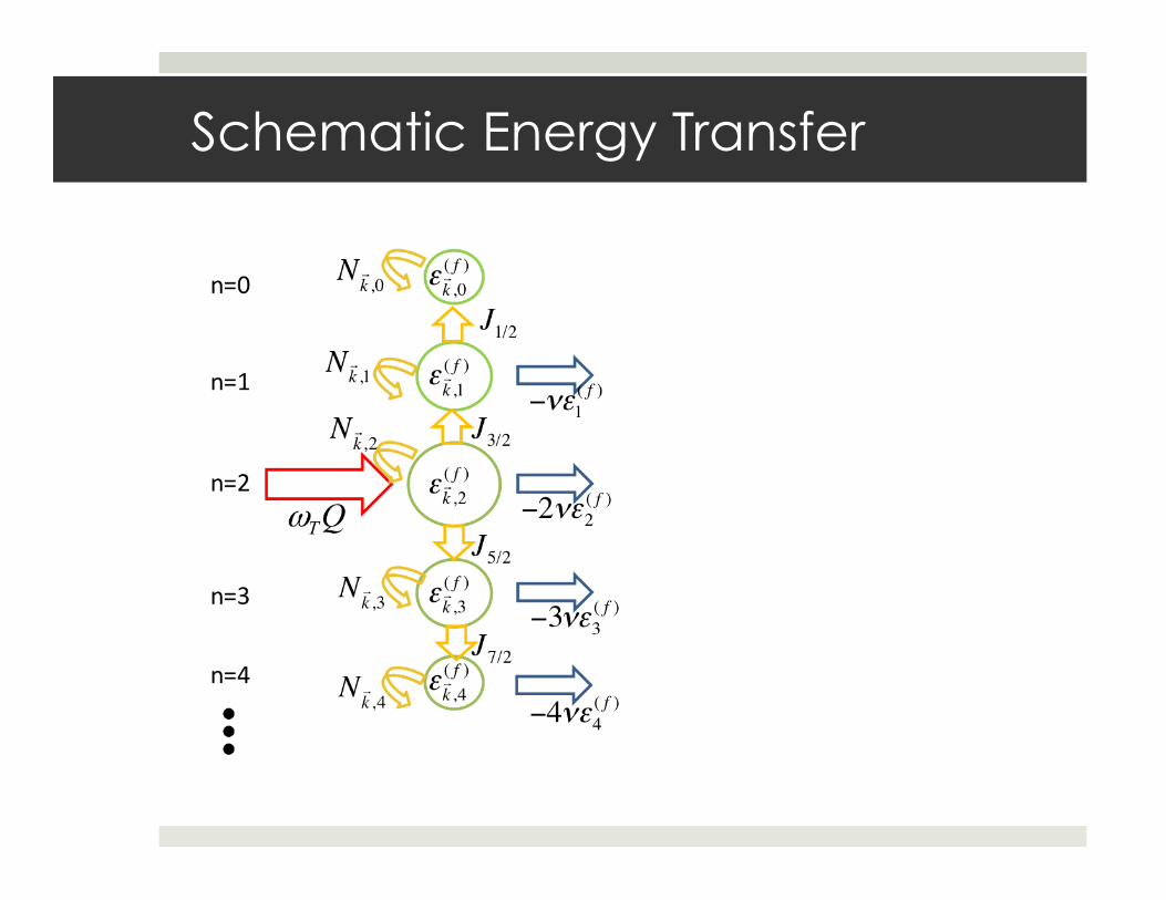
Schematic Energy Transfer

Free Energy

3

D(k⊥) ≡1 + δky,0δkz,0∆/(1− Γ0(k2x))

τ + 1− Γ0(k2⊥)(13)

φ = π14 e−k2

⊥/2D(k⊥)f0 (14)


Q = −π1/4

√2

�

kx,ky,kz

ikyφf∗2 . (15)





π12 fn + π

14 φδn,0

�∗Xn

�. (16)

The free energy is,

εk,n = ε(f)k,n + ε(φ)k δn,0, (17)


ε(f)k,n ≡ 1

2π

12 |fk,n|2, (18)


ε(φ)k ≡ 1

2D(k⊥)|φk|2 (19)

ε(φ)k /ε(f)k,0 = e−k2⊥D(k⊥). (20)



∂ε(φ)k∂t

= J (φ)k +N (φ)

k , (21)

where

J (φ)k ≡ �

�−ikzπ

14 φ∗fk,1

�, (22)

and

N (φ)k ≡ �

��

k�T (φ)

k,k’

�, (23)



�y)φ

∗k φk� f0,k−k� . (24)

3

D(k⊥) ≡1 + δky,0δkz,0∆/(1− Γ0(k2x))

τ + 1− Γ0(k2⊥)(13)

φ = π14 e−k2

⊥/2D(k⊥)f0 (14)


Q = −π1/4

√2

�

kx,ky,kz

ikyφf∗2 . (15)





π12 fn + π

14 φδn,0

�∗Xn

�. (16)

The free energy is,

εk,n = ε(f)k,n + ε(φ)k δn,0, (17)


ε(f)k,n ≡ 1

2π

12 |fk,n|2, (18)


ε(φ)k ≡ 1

2D(k⊥)|φk|2 (19)

ε(φ)k /ε(f)k,0 = e−k2⊥D(k⊥). (20)



∂ε(φ)k∂t

= J (φ)k +N (φ)

k , (21)

where

J (φ)k ≡ �

�−ikzπ

14 φ∗fk,1

�, (22)

and

N (φ)k ≡ �

��

k�T (φ)

k,k’

�, (23)



�y)φ

∗k φk� f0,k−k� . (24)

3

D(k⊥) ≡1 + δky,0δkz,0∆/(1− Γ0(k2x))

τ + 1− Γ0(k2⊥)(13)

φ = π14 e−k2

⊥/2D(k⊥)f0 (14)


Q = −π1/4

√2

�

kx,ky,kz

ikyφf∗2 . (15)





π12 fn + π

14 φδn,0

�∗Xn

�. (16)

The free energy is,

εk,n = ε(f)k,n + ε(φ)k δn,0, (17)


ε(f)k,n ≡ 1

2π

12 |fk,n|2, (18)


ε(φ)k ≡ 1

2D(k⊥)|φk|2 (19)

ε(φ)k /ε(f)k,0 = e−k2⊥D(k⊥). (20)



∂ε(φ)k∂t

= J (φ)k +N (φ)

k , (21)

where

J (φ)k ≡ �

�−ikzπ

14 φ∗fk,1

�, (22)

and

N (φ)k ≡ �

��

k�T (φ)

k,k’

�, (23)



�y)φ

∗k φk� f0,k−k� . (24)

Free energy equations:

Energy Evolution

3

D(k⊥) ≡1 + δky,0δkz,0∆/(1− Γ0(k2x))

τ + 1− Γ0(k2⊥)(13)

φ = π14 e−k2

⊥/2D(k⊥)f0 (14)


Q = −π1/4

√2

�

kx,ky,kz

ikyφf∗2 . (15)





π12 fn + π

14 φδn,0

�∗Xn

�. (16)

The free energy is,

εk,n = ε(f)k,n + ε(φ)k δn,0, (17)


ε(f)k,n ≡ 1

2π

12 |fk,n|2, (18)


ε(φ)k ≡ 1

2D(k⊥)|φk|2 (19)

ε(φ)k /ε(f)k,0 = e−k2⊥D(k⊥). (20)



∂ε(φ)k∂t

= J (φ)k +N (φ)

k , (21)

where

J (φ)k ≡ �

�−ikzπ

14 φ∗fk,1

�, (22)

and

N (φ)k ≡ �

��

k�T (φ)

k,k’

�, (23)



�y)φ

∗k φk� f0,k−k� . (24)

3

D(k⊥) ≡1 + δky,0δkz,0∆/(1− Γ0(k2x))

τ + 1− Γ0(k2⊥)(13)

φ = π14 e−k2

⊥/2D(k⊥)f0 (14)


Q = −π1/4

√2

�

kx,ky,kz

ikyφf∗2 . (15)





π12 fn + π

14 φδn,0

�∗Xn

�. (16)

The free energy is,

εk,n = ε(f)k,n + ε(φ)k δn,0, (17)


ε(f)k,n ≡ 1

2π

12 |fk,n|2, (18)


ε(φ)k ≡ 1

2D(k⊥)|φk|2 (19)

ε(φ)k /ε(f)k,0 = e−k2⊥D(k⊥). (20)



∂ε(φ)k∂t

= J (φ)k +N (φ)

k , (21)

where

J (φ)k ≡ �

�−ikzπ

14 φ∗fk,1

�, (22)

and

N (φ)k ≡ �

��

k�T (φ)

k,k’

�, (23)



�y)φ

∗k φk� f0,k−k� . (24)

3

D(k⊥) ≡1 + δky,0δkz,0∆/(1− Γ0(k2x))

τ + 1− Γ0(k2⊥)(13)

φ = π14 e−k2

⊥/2D(k⊥)f0 (14)


Q = −π1/4

√2

�

kx,ky,kz

ikyφf∗2 . (15)





π12 fn + π

14 φδn,0

�∗Xn

�. (16)

The free energy is,

εk,n = ε(f)k,n + ε(φ)k δn,0, (17)


ε(f)k,n ≡ 1

2π

12 |fk,n|2, (18)


ε(φ)k ≡ 1

2D(k⊥)|φk|2 (19)

ε(φ)k /ε(f)k,0 = e−k2⊥D(k⊥). (20)



∂ε(φ)k∂t

= J (φ)k +N (φ)

k , (21)

where

J (φ)k ≡ �

�−ikzπ

14 φ∗fk,1

�, (22)

and

N (φ)k ≡ �

��

k�T (φ)

k,k’

�, (23)



�y)φ

∗k φk� f0,k−k� . (24)

3

D(k⊥) ≡1 + δky,0δkz,0∆/(1− Γ0(k2x))

τ + 1− Γ0(k2⊥)(13)

φ = π14 e−k2

⊥/2D(k⊥)f0 (14)


Q = −π1/4

√2

�

kx,ky,kz

ikyφf∗2 . (15)





π12 fn + π

14 φδn,0

�∗Xn

�. (16)

The free energy is,

εk,n = ε(f)k,n + ε(φ)k δn,0, (17)


ε(f)k,n ≡ 1

2π

12 |fk,n|2, (18)


ε(φ)k ≡ 1

2D(k⊥)|φk|2 (19)

ε(φ)k /ε(f)k,0 = e−k2⊥D(k⊥). (20)



∂ε(φ)k∂t

= J (φ)k +N (φ)

k , (21)

where

J (φ)k ≡ �

�−ikzπ

14 φ∗fk,1

�, (22)

and

N (φ)k ≡ �

��

k�T (φ)

k,k’

�, (23)



�y)φ

∗k φk� f0,k−k� . (24)

4


∂ε(f)k,n


k δn,1 + Jk,n−1/2 − Jk,n+1/2 +N (f)k . (25)


ηiQ = ��−π1/4

√2ηiikye

−k2⊥/2f∗

2φ

�, (26)


Jk,n−1/2 ≡ ��−π

12 ikz

√nf∗

k,nfk,n−1

�, (27)

and

Jk,n+1/2 ≡ ��π

12 ikz

√n+ 1f∗

k,nfk,n+1

�, (28)


N (f)k,n ≡ �

��

k�T (f)

k,k’,n

�, (29)



�y)f

∗k,nφk−k� fk�,n. (30)




γL ≡J (φ)

k − Jk,1/2

2εk,0(31)

ωnl ∼ kzvTi (32)



γlinγL,lin

γL,nl

kzvTi

4


∂ε(f)k,n


k δn,1 + Jk,n−1/2 − Jk,n+1/2 +N (f)k . (25)


ηiQ = ��−π1/4

√2ηiikye

−k2⊥/2f∗

2φ

�, (26)


Jk,n−1/2 ≡ ��−π

12 ikz

√nf∗

k,nfk,n−1

�, (27)

and

Jk,n+1/2 ≡ ��π

12 ikz

√n+ 1f∗

k,nfk,n+1

�, (28)


N (f)k,n ≡ �

��

k�T (f)

k,k’,n

�, (29)



�y)f

∗k,nφk−k� fk�,n. (30)




γL ≡J (φ)

k − Jk,1/2

2εk,0(31)

ωnl ∼ kzvTi (32)



γlinγL,lin

γL,nl

kzvTi

4


∂ε(f)k,n


k δn,1 + Jk,n−1/2 − Jk,n+1/2 +N (f)k . (25)


ηiQ = ��−π1/4

√2ηiikye

−k2⊥/2f∗

2φ

�, (26)


Jk,n−1/2 ≡ ��−π

12 ikz

√nf∗

k,nfk,n−1

�, (27)

and

Jk,n+1/2 ≡ ��π

12 ikz

√n+ 1f∗

k,nfk,n+1

�, (28)


N (f)k,n ≡ �

��

k�T (f)

k,k’,n

�, (29)



�y)f

∗k,nφk−k� fk�,n. (30)




γL ≡J (φ)

k − Jk,1/2

2εk,0(31)

ωnl ∼ kzvTi (32)



γlinγL,lin

γL,nl

kzvTi

4


∂ε(f)k,n


k δn,1 + Jk,n−1/2 − Jk,n+1/2 +N (f)k . (25)


ηiQ = ��−π1/4

√2ηiikye

−k2⊥/2f∗

2φ

�, (26)


Jk,n−1/2 ≡ ��−π

12 ikz

√nf∗

k,nfk,n−1

�, (27)

and

Jk,n+1/2 ≡ ��π

12 ikz

√n+ 1f∗

k,nfk,n+1

�, (28)


N (f)k,n ≡ �

��

k�T (f)

k,k’,n

�, (29)



�y)f

∗k,nφk−k� fk�,n. (30)




γL ≡J (φ)

k − Jk,1/2

2εk,0(31)

ωnl ∼ kzvTi (32)



γlinγL,lin

γL,nl

kzvTi

4


∂ε(f)k,n


k δn,1 + Jk,n−1/2 − Jk,n+1/2 +N (f)k . (25)


ηiQ = ��−π1/4

√2ηiikye

−k2⊥/2f∗

2φ

�, (26)


Jk,n−1/2 ≡ ��−π

12 ikz

√nf∗

k,nfk,n−1

�, (27)

and

Jk,n+1/2 ≡ ��π

12 ikz

√n+ 1f∗

k,nfk,n+1

�, (28)


N (f)k,n ≡ �

��

k�T (f)

k,k’,n

�, (29)



�y)f

∗k,nφk−k� fk�,n. (30)




γL ≡J (φ)

k − Jk,1/2

2εk,0(31)

ωnl ∼ kzvTi (32)



γlinγL,lin

γL,nl

kzvTi

4


∂ε(f)k,n


k δn,1 + Jk,n−1/2 − Jk,n+1/2 +N (f)k . (25)


ηiQ = ��−π1/4

√2ηiikye

−k2⊥/2f∗

2φ

�, (26)


Jk,n−1/2 ≡ ��−π

12 ikz

√nf∗

k,nfk,n−1

�, (27)

and

Jk,n+1/2 ≡ ��π

12 ikz

√n+ 1f∗

k,nfk,n+1

�, (28)


N (f)k,n ≡ �

��

k�T (f)

k,k’,n

�, (29)



�y)f

∗k,nφk−k� fk�,n. (30)




γL ≡J (φ)

k − Jk,1/2

2εk,0(31)

ωnl ∼ kzvTi (32)



γlinγL,lin

γL,nl

kzvTi

Electrostatic part:

Entropy part:

application of proper orthogonal decomposition to analysis ...kunz/site/pcts_files/modeling rotating...

Documents