application of recent optimization algorithms on …

APPLICATION OF RECENT OPTIMIZATION ALGORITHMS ON SLOPE

STABILITY PROBLEMS

A THESIS SUBMITTED TO

THE GRADUATE SCHOOL OF NATURAL AND APPLIED SCIENCES

OF

MIDDLE EAST TECHNICAL UNIVERSITY

BY

SADRA AZIZI

IN PARTIAL FULFILLMENT OF THE REQUIREMENTS

FOR

THE DEGREE OF MASTER OF SCIENCE

IN

CIVIL ENGINEERING

JULY 2018

Approval of the thesis:

APPLICATION OF RECENT OPTIMIZATION ALGORITHMS ON

SLOPE STABILITY PROBLEMS

submitted by SADRA AZIZI in partial fulfillment of the requirements for the

degree of Master of Science in Civil Engineering Department, Middle East

Technical University by,

Prof. Dr. Halil Kalıpçılar

Dean, Graduate School of Natural and Applied Sciences

Prof. Dr. İsmail Özgür Yaman

Head of Department, Civil Engineering

Asst. Prof. Dr. Onur Pekcan

Supervisor, Civil Engineering Dept., METU

Examining Committee Members:

Prof. Dr. Bahadır Sadık Bakır

Civil Engineering Dept., METU

Asst. Prof. Dr. Onur Pekcan


Prof. Dr. Oğuzhan Hasançebi


Assoc. Prof. Dr. Zeynep Gülerce


Asst. Prof. Dr. Salih Tileylioğlu

Civil Engineering Dept., Çankaya University

Date: 18.07.2018

iv

I hereby declare that all information in this document has been obtained and

presented in accordance with academic rules and ethical conduct. I also

declare that, as required by these rules and conduct, I have fully cited and

referenced all material and results that are not original to this work.

Name, Last Name: Sadra Azizi

Signature:

v

ABSTRACT

APPLICATION OF RECENT OPTIMIZATION ALGORITHMS ON

SLOPE STABILITY PROBLEMS

Azizi, Sadra

M.Sc., Department of Civil Engineering

Supervisor: Assist. Prof. Dr. Onur Pekcan

July 2018, 107 pages

Stability analysis of earth slopes in general involves determining the minimum

factor of safety (FS) associated with the most critical failure surface. This objective

is too challenging to accomplish considering the broad diversity of slope problems

in geometry, geotechnical parameters of the soil, location of the groundwater table,

and condition of the external loadings. Robust optimization techniques, however,

have recently performed well in determining safety factors of various man-made

and natural slopes of different complexities simultaneous with fast and confidently

locating the corresponding slip surfaces.

In this study, three recently developed optimization methods, Hybrid Artificial Bee

Colony algorithm with Differential Evolution (HABCDE), Grasshopper

Optimization Algorithm (GOA) and improved harmony search algorithm (LHS),

are combined with a non-circular surface generation scheme to identify location of

the slip surface. To evaluate the safety factor along each slip surface, a concise

algorithm of the Morgenstern-Price method is employed in the analyses. Results

obtained through application of the proposed methods into three case studies

including different layers and geometries indicates that HABCDE outperforms the

two other methods both on fast convergence and accuracy in the minimization

vi

procedure which makes it comparable to the best methods implemented in slope

stability analysis to date.

Keywords: Geotechnical Engineering, Slope Stability, Critical Slip Surface,

Metaheuristic Methods, Factor of Safety

vii

ÖZ

ŞEV STABILITE ANALIZLERININ OPTIMIZASYON

TEKNIKLERI KULLANILARAK DEĞERLENDIRILMESI

Azizi, Sadra

Yüksek Lisans, İnşaat Mühendisliği Bölümü

Tez Yöneticisi: Dr. Öğr. Üyesi Onur Pekcan

Temmuz 2018, 107 sayfa

Şevlerin duraylılık analizi, en kritik kayma yüzeyi ile en düşük güvenlik faktörünün

(GF) belirlenmesini içerir. Bu amaçla yapılan çalışmalar, geometrik eğim çeşitliliği,

toprağın geoteknik parametreleri, yeraltı suyu seviyesinin yeri ve harici yüklerin

durumu göz önünde bulundurulduğunda oldukça zor bir problem haline

gelmektedir. Bununla birlikte son zamanlarda, güçlü optimizasyon teknikleri farklı

kayma yüzeylerinin çeşitli insan yapımı ve doğal eğimlerin güvenlik faktörlerinin

belirlenmesinde, hızlı ve güvenli bir şekilde belirlenmesinde iyi bir performans

sergilemiştir.

Bu çalışmada, şev kayma yüzeyi ve güvenlik faktörünü belirlemek için Ayırıcı

Evrimli Hibrit Yapay Arı Kolonisi algoritması (AEHYAKA), Çekirge

Optimizasyon Algoritması (ÇOA) ve Geliştirilmiş Uyum Arama Algoritmasını

(GUAA) içeren üç yeni optimizasyon yöntemi dairesel olmayan bir yüzey

oluşturma algoritması ile birleştirilmiştir. Her bir kayma yüzeyi boyunca güvenlik

faktörünü değerlendirmek için yapılan analizlerde Morgenstern-Price metodu

algoritması kullanılmıştır. Önerilen metotların, farklı katmanlar ve geometri içeren

3 örnek çalışma ile uygulanması sonucu elde edilen sonuçlar, AEHYAKA 'nin, hem

hızlı yakınsama hem de doğruluk açısından diğer iki yöntemi geride bıraktığını ve

viii

bu durumun şev stabilitesi analizinde bugüne kadar uygulanan en iyi yöntemlerle

karşılaştırılabilir olduğunu göstermektedir.

Anahtar Kelimeler: Geoteknik mühendisliği, Şev Stabilitesi, Kritik Kayma Yüzeyi,

Sezgi Ötesi Yöntemler, Güvenlik Faktörü

ix

To My Family

x

ACKNOWLEDGMENTS

This thesis was written with the help and assistance of various people and I would

like to take this opportunity to acknowledge the tremendous help they have given

me while I was completing my thesis.

First and foremost, I would like to express my sincere appreciation and gratitude to

my advisor, Dr. Onur Pekcan, whose enlightening remarks, encouraging feedback

and friendly attitude all year long, made this dissertation possible. Dr. Pekcan has

been both my dissertation adviser and my mentor, providing me with endless

encouragement and helping me go through all the difficulties I came across as a

student and a researcher. He was very generous in sharing his experiences in

academic life and beyond which made the biggest positive difference in my life.

I would also like to thank the examining committee members Dr. Bahadır Sadık

Bakır, Dr. Oğuzhan Hasançebi, Dr. Zeynep Gülerce and Dr. Salih Tileylioğlu for

spending their valuable time on reviewing my thesis and providing feedback.

I would like to express my sincere and special gratitude to my family for their

constant care and understanding, encouragement and endless love throughout my

life. I have always felt their supports even if I had been away from them. Without

their unconditional trust, timely encouragement, and endless patience throughout

my life, I could not be who I am now.

I owe special thanks to my wonderful cousin Hamed Ahmadzadeh for his

invaluable assistance and encouragements, his thoughts, phone calls and visits

throughout my study. He has always been like a brother to me and one of the

greatest supporters in my life. I also want to express my great appreciation to Taher

Ghalandary, Navid Alamati, Majid Jarrah and Mohammad Reza Kolahi for their

valuable friendship, endless support and being there whenever I needed a friend.

xi

I would also like to acknowledge my colleagues, Reza Salatin, Farshad Kamran,

Ali Farshkaran, Armin Taghipour, Rasoul Tariverdilou and my fellow AI2LAB

members for their valuable friendship and support during my thesis journey

xiii

TABLE OF CONTENTS

ABSTRACT ............................................................................................................ v

ÖZ ....................................................................................................................... vii

ACKNOWLEDGMENTS ....................................................................................... x

TABLE OF CONTENTS ..................................................................................... xiii

LIST OF TABLES ................................................................................................ xv

LIST OF FIGURES .............................................................................................. xvi

LIST OF ABBREVIATIONS .............................................................................. xix

CHAPTERS

1. INTRODUCTION ........................................................................................... 1

1.1. Background .............................................................................................. 1

1.2. Research Objective ................................................................................... 5

1.3. Scope ........................................................................................................ 6

1.4. Thesis Outline ........................................................................................... 7

2. LITERATURE WORK ................................................................................... 9

2.1 Slope Stability Analysis Methods ............................................................... 9

2.1.1 Limit Equilibrium Methods ............................................................ 10

2.1.2 Numerical Methods ......................................................................... 16

2.2 Current Challenges .................................................................................... 18

2.3 Determination of the Critical Failure Surface ........................................... 19

2.3.1 Differential evolution ...................................................................... 21

2.3.2 Harmony Search ............................................................................. 24

2.3.3 Artificial Bee Colony ..................................................................... 26

3. MAIN WORK ............................................................................................... 29

3.1 Trial Slip Surface Generation Method ...................................................... 29

3.2 Calculation of Factor of Safety ................................................................. 31

3.3 Optimization Methods ............................................................................... 37

xiv

3.3.1 Improved harmony search algorithm .............................................. 38

3.3.2 Grasshopper optimization algorithm .............................................. 44

3.3.3 Hybrid Artificial Bee Colony with Differential Evolution ............. 47

4. CASE STUDIES ............................................................................................ 53

4.1 Case study 1 ............................................................................................... 54

4.2 Case study 2 ............................................................................................... 59

4.3 Case study 3 ............................................................................................... 65

4.4 Case Study 4 .............................................................................................. 74

5. SUMMARY AND CONCLUSION ............................................................... 89

5.1 Summary .................................................................................................... 89

5.2 Findings of the Study ................................................................................. 90

5.3 Future Works ............................................................................................. 91

REFERENCES ...................................................................................................... 93

APPENDIX

A: CONVERGENCE RATE COMPARISON ...................................................... 99

xv

LIST OF TABLES

TABLES

Table 1 - Summary of Limit equilibrium methods ............................................... 16

Table 2 - Result Comparison – Example 1 ........................................................... 55

Table 3 - Results of this study—Example 1.......................................................... 56

Table 4 - Soil Parameters – Example 2 ................................................................. 60

Table 5 - Result comparison—Example 2 ............................................................ 61

Table 6 - Results of this study—Example 2.......................................................... 62

Table 7 - Soil parameters—Example 3 ................................................................. 66

Table 8 - Result comparison—Example 3 ............................................................ 67

Table 9 - Results of this study—Example 3, Case (1) .......................................... 68

Table 10 - Results of this study—Example 3, Case (2) ........................................ 72

Table 11 - Soil Parameters – Example 4 ............................................................... 75

Table 12 - Result Comparison – Example 4 ......................................................... 76

Table 13 - Results of this study—Example 4........................................................ 77

xvi

LIST OF FIGURES

FIGURES

Figure 1 - Taiwan freeway landslide ....................................................................... 2

Figure 2 - Banjarnegara, Indonesia landslide .......................................................... 3

Figure 3 - Forces applied on the sample slice ....................................................... 12

Figure 4 – Forces applied on the sample slice ....................................................... 13




Figure 8- Geometric Description of the Surface Generation Method ................... 31

Figure 9 - (a) Slope Geometry and General Failure Surface, (b) Inter-Slice Forces

in Slice Number (i) ................................................................................................ 33

Figure 10 - Flowchart of FS Algorithm ................................................................. 36

Figure 11 - Two main branches about the improvisation process ........................ 42

Figure 12 - LHS Algorithm ................................................................................... 43

Figure 13 - GOA Algorithm .................................................................................. 47

Figure 14 - HABCDE Algorithm .......................................................................... 51

Figure 15 - Flowchart for HABCDE Algorithm ................................................... 52

Figure 16 - Slope geometry—Example 1 .............................................................. 54

Figure 17 - Comparison of the convergence rates -- Example 1 (a) all the methods

(b) proposed methods ............................................................................................ 58

Figure 18 - Critical Slip Surfaces -- Example 1 .................................................... 59

Figure 19 - Geometry of Slope – Example 2 ......................................................... 60


(b) proposed methods ............................................................................................ 64

Figure 21 - Critical Slip Surfaces -- Example 2 .................................................... 65

Figure 22 - Geometry of Slope—Example 3 ......................................................... 66

xvii

Figure 23 - Comparison of the convergence rates -- Example 3, Case (1) (a) all

the methods (b) proposed methods ....................................................................... 70

Figure 24 - Critical Slip Surfaces —Example 3, Case (1) .................................... 71



Figure 26 - Critical Slip Surfaces —Example 3, Case (2) .................................... 74

Figure 27 - Geometry of the slope – Example 4 ................................................... 75

Figure 28 Comparison of the convergence rates -- Example 4, Case (1) (a) all the

methods (b) proposed methods ............................................................................. 81







Figure 32 – Critical Slip Surfaces – Example 4 .................................................... 87

Figure 33- Convergence Rate Comparison – Example 1 .................................... 100

Figure 34 - Convergence Rate Comparison – Example 2 ................................... 101

Figure 35 - Convergence Rate Comparison – Example 3, Case (1) ................... 102






xix

LIST OF ABBREVIATIONS

ABBREVIATION

ABC Artificial Bee Colony

ACO Ant Colony Optimization

DE Differential Evolution

DEM Distinct Element Method

DFP Davidon-Fletcher-Powell

FDM Finite Difference Method

FEM Finite Element Method

FS Factor of Safety

GA Genetic Algorithms

GOA Grasshopper Optimization Algorithm

GSA Gravitational Search Algorithm

HABCDE Hybrid Artificial Bee Colony Algorithm with Differential

Evolution

HM Harmony Memory

HMCR Harmony Memory Consideration Rate

HMS Harmony Memory Size

HS Harmony Search

ICA Imperialistic Competitive Algorithm

LEM Limit Equilibrium Method

xx

LHS Improved Harmony Search Algorithm

M-P Morgenstern-Price Method

MHM Modified Harmony Search Algorithm

PAR Pitch Adjusting Rate

PPACO Premium-Penalty Ant Colony Optimization

PSO Particle Swarm Optimization

SA Simulated Annealing

SHM Simple Harmony Search Algorithm

SRM Strength Reduction Method

1

CHAPTER 1

1.INTRODUCTION

1.1. Background

Recent growth in human population has led to an increasing demand on major

infrastructure projects such as constructions of roads and railways or buildings,

which generally involve ground disturbance in the area of construction. In many

cases, large-scale earthwork activities require forming engineered cut and fill slopes

prior to any further developments. Therefore, the stability of slopes needs to be

assessed in advance to construction to gain insights about the site conditions as well

as to decrease the risk of having potential property damages and more importantly

human losses.

Slope failures are commonly investigated type of geo-hazards, triggered by

different major causes including intense rainfalls, inadequate drainage, sudden

ground vibrations, loss of vegetation, etc., which eventually result in either an

increase in the stress applied, or cause a reduction in the shear strength of the soil

in situ. The incidence of slope failures may potentially lead to considerable

environmental, financial and human losses, most notably in populated urban areas.

Such ground instabilities may also hinder further progress in the construction

activities and challenge the engineers in charge of the construction.

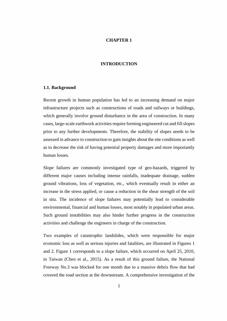
Two examples of catastrophic landslides, which were responsible for major

economic loss as well as serious injuries and fatalities, are illustrated in Figures 1

and 2. Figure 1 corresponds to a slope failure, which occurred on April 25, 2010,

in Taiwan (Chen et al., 2015). As a result of this ground failure, the National

Freeway No.3 was blocked for one month due to a massive debris flow that had

covered the road section at the downstream. A comprehensive investigation of the

2

area demonstrated that weathering had occurred at the upper layers which had

increased the water infiltration into the soil and consequently had led to water

accumulation between the layers. As a result, the decline in interface friction

resulted in slope instability in this area (Chen et al., 2015).

Figure 1 - Taiwan freeway landslide (Taiwan National Freeway Bureau)

Figure 2 represents another devastating landslide occurred on December 13, 2014,

in Indonesia. As a result of this disaster, a large number of houses in the area were

heavily damaged and the total number of fatalities and injuries was considerable.

Comprehensive site investigations revealed that heavy rainfall in a short period of

time (11 days) in addition to the steep configuration of the slope were the major

causes and the triggering factors of the ground failure (Nur, 2014).

Considering the possible outcomes, in regions of high failure risks, large amounts

of money are yearly invested in the proper maintenance of major geotechnical

structures such as embankments or dams and in the design of man-made facilities

adjacent to slopes. Therefore, studies related to better understanding of the stability

of slopes play a crucial role especially from economy and sustainability point of

view.

3

Figure 2 - Banjarnegara, Indonesia landslide (Nur, 2014)

To date, considerable efforts have been made to evaluate the stability of earth slopes

of different configurations under various loading conditions prior to major

constructions adjacent to slopes, and to take necessary actions to improve the

stability of slopes in areas of high failure risk. For this purpose, different numerical

and analytical methods including, limit analysis method, limit equilibrium method

(LEM), finite difference method or finite element method, have been so far

developed by the researchers in order to properly assess the stability of slopes.

However, studies indicate that LEM is as yet the most popular approach among the

researchers for stability analyses. Over the past few years, a set of LEM based

techniques that vary in their underlying assumptions has been widely utilized in

different stability assessment problems.

Stability of slopes in LEM is precisely quantified using a term so-called “Factor of

Safety” (“FS”), which indicates the ratio between the existing shear strength and

the shear stress acting on the sliding body. However, an accurate safety assessment

by using LEMs requires a number of trial slip surfaces to be initially generated

4

followed by calculation of the value of factor of safety corresponding to each slip

surface and finally indicating the surface with the lowest FS value as the surface of

highest failure probability for the entire slope. However, indicating the most critical

slip surface would remain challenging for engineers, as far as the accuracy of the

approximations along with the time required for the completion of the computations

are concerned.

This objective can be achieved following a trial and error approach. Although

useful, this method lacks precision particularly in the case of nonhomogeneous soil

slopes. The incompetency in this method is however associated with its dependency

on the adequacy of the preliminarily generated trial failure surfaces within the slope

profile. Considering the fact that the critical slip surface identified by using the

approach is not necessarily the most vulnerable surface, inappropriate values are

therefore likely to be obtained in the analyses.

Alternatively, available evidence from published case studies, have demonstrated

the capability of optimization techniques in the reliable assessment of the stability

of slopes. To date, different classical optimization methods have been implemented

in the analyses. These techniques, considering their inherent limitations, are also

proved to be dependent on the proper selection of trial solutions and thus might also

overestimate the value of safety factor and consequently fail to acquire a precise

measure in the analyses. However, recent advances in computing science have

paved the way for the development of enhanced computing schemes such as

metaheuristics, which have proved successful in solving various real problems.

Successful application of such optimization techniques has recently, gained

significant attention by geotechnical researchers worldwide (Yung Ming Cheng et

al., 2012). To date, a broad range of novel optimization methods has been used in

the literature to explore the most vulnerable failure surface as well as to determine

the factor of safety against instabilities in the case of study. Review of the results

obtained for these methods testify their competence in better evaluating the stability

of earth slopes given the improvements made in the obtained results. Particularly

when applied to a multi-layered slope with a complex geometry, the optimization

5

technique is required to accurately locate the geological slip surface, over a short

period with relatively less computational efforts. Consequently, this objective

necessitates the use of alternative optimization techniques in order to obtain

superior results, especially for complex case studies.

In this study, an effective analysis framework is developed implementing three

recently developed metaheuristic methods, combined with a simplified

Morgenstern-Price approach so as to determine the minimum factor of safety

pertaining to the most critical slip surface within the soil profile. Subsequently, the

proposed framework is utilized in stability analysis of four slope problems with

various complexities and its performance is benchmarked against its conventional

competitors.

1.2. Research Objective

This study primarily intends to develop a functional analysis framework to assess

the factor of safety of earth slopes on the basis of limit equilibrium methods.

However, the formulation derived for the factor of safety in an advanced LEM, such

as Morgenstern-Price method, suffers from specific drawbacks, i.e. discontinuity

and the existence of several local minima (Chen et al. 1988, Cheng et al. 2007) that

make slope stability analysis a challenging problem to solve. To successfully deal

with this problem, limit equilibrium methods coupled with various metaheuristic

optimization techniques are employed in the analyses. In this regard, the factor of

safety equation is generally considered as the objective function of the optimization

problem and a thorough minimization process is performed to explore the optimum

solution in the search space. An overall evaluation regarding the safety of the case

of study can be reached after the analyses are completed.

Another major objective of this study is the fast and accurate localization of the

critical slip surface that yields the minimum factor of safety of the entire slope.

Having determined the zone with high failure risk, necessary actions need to be

taken to reinforce the vulnerable surface with its surroundings.

6

1.3. Scope

Studies thus far have firmly indicated the significance of the meticulous

geometrical modeling of the soil in situ, on the validity of the slope stability

assessments. A number of major factors found to be influencing the analyses

include: the geometry of the slope, consideration of the existence of water table

along with the external loadings in the analyses, and above all the validity of the

values assumed for the soil parameters. Accordingly, these aspects are required to

be considered in the calculations for more realistic results to be acquired.

Investigations have established the direct role undesirable conditions within the soil

profile, e.g., the presence of a weak layer, play in activating the failure mechanism

of the slopes. In this study, various case of studies from simple homogeneous to

multi-layered heterogeneous earth slopes with varied geometries and stratifications

are considered, in order to better investigate the impact of variation in ground

conditions on the overall stability of slopes. Furthermore, a deterministic approach

is adopted for the analyses considering constant values for the key parameters of

the soil medium, namely coefficient of cohesion, unit weight, friction angle, and

pore water pressure ratio within each of the layers.

Available evidence of ground failures in areas with high precipitation rate has

indicated the adverse influence of the pore water pressure on the soil strength. In

this study, the destabilizing effects of external loadings and ground water table as

well as the combined effects of these parameters on the stability condition of two

case studies, are efficiently investigated.

Other slope stability evaluation techniques including finite element method (FEM)

are kept out of the scope of this study. Although powerful, FEM is generally not

adopted for the analysis of typical geotechnical problems owing to the difficulties

involved in an accurate modeling of the problem along with a large number of

parameters required to be initialized in the analysis.

7

1.4. Thesis Outline

This study consists of five themed chapters, starting with this introductory chapter.

Subsequent chapters are organized as follows: The second chapter is devoted to

literature work associated with slope stability analysis methods, current challenges,

and optimization techniques. In the third chapter, the main work of the study,

including the method used for generating trial slip surfaces and the adopted

optimization algorithms are explained in details. In the fourth chapter, the

application of the proposed method on benchmark case studies have been

exemplified and the last chapter includes the conclusions of this study and identifies

areas for the future work.

9

CHAPTER 2

2.LITERATURE WORK

This chapter provides an overview of the practical methods introduced thus far for

the stability analysis of earth slopes in a two-dimensional space. In this regard,

formulation of a number of widely-known techniques that are developed on the

basis of limit equilibrium methods (LEM) or finite element methods (FEM) is

detailed. Furthermore, recent challenges and essential considerations in an

exhaustive slope stability assessment are briefly addressed in this chapter. Finally,

a summary of the techniques used in the literature for tackling the difficulties in

identifying the most vulnerable failure surface within the slope is provided.

2.1 Slope Stability Analysis Methods

To date, considerable efforts have been made to evaluate the stability of earth slopes

of different configuration under various loading conditions prior to major

constructions adjacent to slopes, and to take necessary actions to improve the

stability of slopes in areas of high failure risk. For this purpose, different numerical

and analytical methods including, limit analysis method, limit equilibrium method

(LEM), finite difference method or finite element method, have been so far

developed by the researchers in order to properly assess the stability of slopes.

However, studies indicate that LEM is as yet the most popular approach among the

researchers for stability analyses. Over the past few years, a set of LEM based

techniques that vary in their underlying assumptions. In the following subsection,

a number of most commonly used techniques pertaining to limit equilibrium

methods are described in detail.

10

2.1.1 Limit Equilibrium Methods (LEM)

Despite the potential drawbacks in each of the methods, LEM is as yet the most

adopted approach since it can be confidently applied to slopes of diverse geometric

shapes comprising different soil characteristics and water content, subjected to

external loading conditions of different kinds. Besides, overall attitude toward LEM

has become favorable due to its relatively straightforward implementation. Limit

equilibrium methods are, for the most part, formed on the basis of the methods of

slices which enjoys the following features as in the study by (D. Y. Zhu et al., 2003):

1. The sliding mass of the soil is ordinarily divided into multiple vertical,

inclined or horizontal slices; however, vertical slices approach is the most

commonly employed technique in the research works to date.

2. The sliding mass above the failure surface is brought into the limiting state,

by evenly mobilizing the strength along the entire surface.

3. Simplifying assumptions concerning inter-slice forces need to be made in

order to solve this statically indeterminate problem.

4. The safety factor is calculated according to the moment and/or force

equilibrium equations.

In order to properly quantify the chance of failure in slopes, an index which is

referred to as factor of safety (FS) is introduced. Factor of safety, in general, is

identified by evaluating the ratio between sum of the forces which resist the

slippage of the soil mass over the failure surface ( resistingF )−friction between soil

particles for instance−and the forces driving the soil mass down the slope ( drivingF

)−such as gravitational forces and external forces, as presented in Equation (1).

( )

( )

resisting

driving

sumof the resisting forces FF

sumof the driving forces F (1)

11

Safety of the earth slopes is determined by comparing the calculated FS values with

a target value which equals unity when the forces acting on the soil mass are

balanced and the slope is in the state of equilibrium. However, a FS value less than

unity indicates a state in which the failure is likely to occur (driving forces >

resisting forces), and in contrast, a value greater than unity for factor of safety,

corresponds to a slope in which the resisting forces outperform the driving forces

and thus, the slope remains stable under the given loading conditions (Duncan et

al., 2014).

As mentioned previously, in limit equilibrium analysis, sliding mass of the soil is

ordinarily divided into multiple vertical slices, so as to specify the forces applied

on each of the slices, i.e., internal and external forces, which are then utilized in

evaluating the safety factor of the case of study. Furthermore, in limit equilibrium

method the value of safety factor is considered to be constant along the failure

surface according to the study by (Y. M Cheng & Lau, 2008); thus, factor of safety

for a single slice represents the safety factor of the whole slope.

Further to the features outlined earlier, limit equilibrium method is regarded as a

statically indeterminate problem and thus far several methods that vary depending

on the simplifying assumptions that are made in modeling the inter-slice forces are

introduced. Among the methods developed for the slope stability analysis, a number

of relatively rigorous ones that has found widespread application in the literature

are briefly outlined below.

2.1.1.1 Ordinary method of slices

The ordinary method of slices which is also known as, Swedish method of slices,

is the primary method of slices introduced for slope stability analysis. The inter-

slice normal and forces in this method are neglected and a surface of circular

geometry is considered for the expected failure surface. Additionally, moment

equilibrium condition is merely met for the body of soil above the slip surface, and

the factor of safety is obtained summing all moments about the center point of the

circle corresponding to the slip surface. This method, while simple, is not precise

12

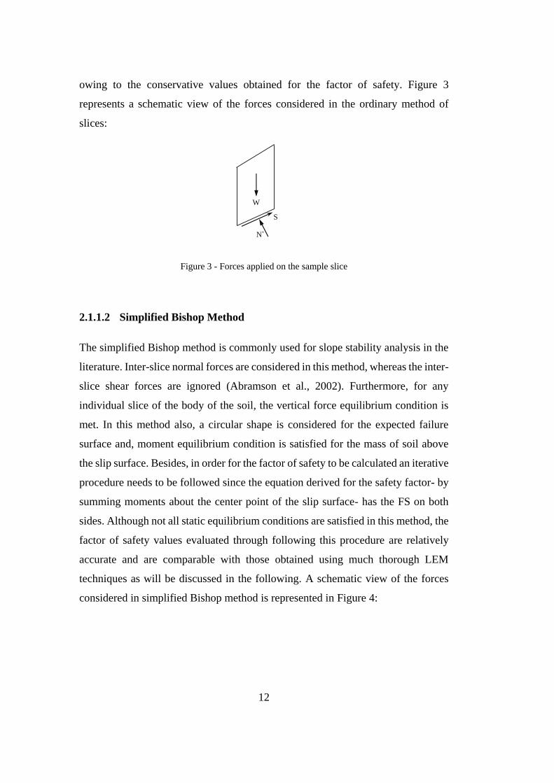
owing to the conservative values obtained for the factor of safety. Figure 3

represents a schematic view of the forces considered in the ordinary method of

slices:

Figure 3 - Forces applied on the sample slice

2.1.1.2 Simplified Bishop Method

The simplified Bishop method is commonly used for slope stability analysis in the

literature. Inter-slice normal forces are considered in this method, whereas the inter-

slice shear forces are ignored (Abramson et al., 2002). Furthermore, for any

individual slice of the body of the soil, the vertical force equilibrium condition is

met. In this method also, a circular shape is considered for the expected failure

surface and, moment equilibrium condition is satisfied for the mass of soil above

the slip surface. Besides, in order for the factor of safety to be calculated an iterative

procedure needs to be followed since the equation derived for the safety factor- by

summing moments about the center point of the slip surface- has the FS on both

sides. Although not all static equilibrium conditions are satisfied in this method, the

factor of safety values evaluated through following this procedure are relatively

accurate and are comparable with those obtained using much thorough LEM

techniques as will be discussed in the following. A schematic view of the forces

considered in simplified Bishop method is represented in Figure 4:

S

W

N '

13

Figure 4 – Forces applied on the sample slice

2.1.1.3 Janbu’s Simplified Method

In the Janbu’s Simplified method, similar to the Bishop’s Simplified method, while

the normal inter-slice forces are considered, inter-slice shear forces are neglected.

However, in this method, unlike Bishop’s simplified method, moment equilibrium

condition is not satisfied and instead, the factor of safety equation is derived from

the horizontal force equilibrium of an individual slice. In addition, a non-circular

geometry is considered for the expected failure surface in this method. In order to

include the influence of inter-slice shear forces on the factor of safety, a correction

factor is introduced which is dependent on the friction angle, the shape of the slip

surface and the cohesion (Janbu, 1975). A schematic view of the forces considered

in simplified Bishop method is represented in Figure 5:


S

E1

E2W

N '

S

E1

E2W

N '

14

2.1.1.4 Morgenstern-Price Method

In the Morgenstern‐Price method (M‐P) both the inter-slice normal and shear

forces, as presented in Figure 6, are considered. Besides, a slip surface of non-

circular shape is considered and for each individual slice of the entire mass of the

soil above the slip surface, two conditions of equilibrium, namely moment as well

as the force equilibrium are satisfied. An inter-slice force function which represents

the ratio of normal forces over shear inter-slice forces is proposed in the M-P

method. This ratio, however, is dependent on a scaling factor λ and, a prescribed

function f(x) that may be assumed of any form such as constant, trapezoidal, half-

sine or a user-defined function.


Due to nonlinearity and complexity of the equilibrium equations, the original M-P

method is highly nonlinear and sophisticated. An alternative formulation which is

easier to implement is developed by (Fredlund & Krahn, 1977). In this regard, two

equations for factor of safety one principally based on the force equilibrium and

another based on the moment equilibrium conditions are derived. Following an

iterative procedure, the corresponding factor of safety can be evaluated. In this

study, a concise and reformulated form of Morgenstern-Price method is adopted for

the slope stability analyses which will be outlined in detail in what follows.

S

E1

E2 W

T1

T2

N '

15

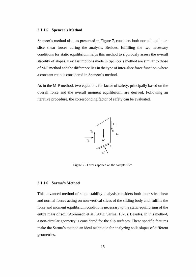
2.1.1.5 Spencer’s Method

Spencer’s method also, as presented in Figure 7, considers both normal and inter-

slice shear forces during the analysis. Besides, fulfilling the two necessary

conditions for static equilibrium helps this method to rigorously assess the overall

stability of slopes. Key assumptions made in Spencer’s method are similar to those

of M-P method and the difference lies in the type of inter-slice force function, where

a constant ratio is considered in Spencer’s method.

As in the M-P method, two equations for factor of safety, principally based on the

overall force and the overall moment equilibrium, are derived. Following an

iterative procedure, the corresponding factor of safety can be evaluated.


2.1.1.6 Sarma’s Method

This advanced method of slope stability analysis considers both inter-slice shear

and normal forces acting on non-vertical slices of the sliding body and, fulfills the

force and moment equilibrium conditions necessary to the static equilibrium of the

entire mass of soil (Abramson et al., 2002; Sarma, 1973). Besides, in this method,

a non-circular geometry is considered for the slip surfaces. These specific features

make the Sarma’s method an ideal technique for analyzing soils slopes of different

geometries.

S

E1

E2 W

T1

T2

N '

16

The procedure followed in the Sarma’s method is different from that of other

methods in that a value is initially assumed for the factor of safety and, efforts are

made to assess the magnitude of a horizontal acceleration which is applied to the

mass of soil above the slip surface to bring it to the point of failure. Consequently,

a relationship between the acceleration and the presumed factor of safety is

developed using which, the static FOS corresponding to a horizontal acceleration

of zero magnitude, is determined (Abramson et al., 2002). Table 1 below, represents

an overview of the limit equilibrium methods that are developed to date.

Table 1 - Summary of Limit equilibrium methods (Pockoski & Duncan, 2000)

2.1.2 Numerical Methods

Despite the extensive use of limit equilibrium methods in slope stability analysis in

practice, many efforts have been made to find alternative schemes which mostly

17

eliminate the need for initial assumptions prior to evaluations, such as the

consideration of probable location and shape for the slip surface in LEM. Another

drawback of these methods, however, is the type of inter-slice forces considered for

each slice within the soil mass (Griffiths & Lane, 1999).

Successful application of numerical in solving various problems in different fields

of engineering has recently drawn increasing attention from geotechnical engineers

worldwide. In the following sections, three numerical approaches that are widely

adopted in the literature, particularly for analyzing complex engineering problems,

are detailed:

2.1.2.1 Finite Element Method (FEM)

Traditional limit equilibrium methods, according to Stead et al. (2001), might fail

to adequately evaluate the slope instabilities, particularly in the case of complex

failure mechanisms, such as internal deformations, brittle fractures, and progressive

failure phenomenon, etc. The reason for this inadequacy lies in the fact that the

stress-strain relationship within the soil medium is not considered in the limit

equilibrium analysis. Adoption of the finite element method, in contrast, provides

important insights into the stress distribution and strain conditions within the soil,

and thus anticipates the deformations in the slope. The soil medium in the FEM

analysis is discretized into small elements that are connected together by nodal

points. The overall distribution of the stresses within the soil can then be completely

determined by calculation of the stresses and strains in these elements, followed by

application of the superposition theorem. Factor of safety in a slope stability

analysis with FEM is commonly calculated by using strength reduction method

(SRM), in which soil strength parameters, namely friction angle (𝜑) and cohesion

(c), are reduced concurrently until the sliding occurs.

2.1.2.2 Finite Difference Method (FDM)

In this approach, like in the finite element method, the soil medium is initially

discretized into various small zones which are connected by the points called

18

Gridpoints. However, stress and deformations in finite difference method can be

merely determined at these gridpoints, while these results are available for any point

within the medium in the finite element method. To date, FDM methods have been

widely implemented in the design process of various geotechnical engineering

infrastructures, as an adequate alternative to traditional limit equilibrium methods,

however, FEM methods are preferred when high accuracy is demanded.

2.1.2.3 Distinct Element Method (DEM)

This numerical method provides geotechnical engineers with important insights

into the mechanism of failure by simulating the stepwise movements of the sliding

body over the course of analysis. In this method, the model used for the soil medium

consists of a large number of arbitrarily shaped discrete particles in which both the

interparticle interactions and the finite movements of the elements are efficiently

considered (Hart, 1995), However, as noted by Cheng et al.(2014), slope stability

analysis using DEM requires much computation time and its sensitivity to

parameters involved in the analysis might hinder its broad application in typical

engineering problems.

2.2 Current Challenges

The appropriate method for analyzing the stability of slopes is, in general, adopted

on the basis of the geometry and classification of the soil mass within the earth

slope, as well as on the basis of the shape expected for the failure surface

(Abramson et al., 2002). Available evidence in the literature reveals that adoption

of different limit equilibrium analysis techniques might result in slight differences

in the value of factor of safety, owing to the variations in the simplifying

assumptions made in each method. Also, in their study of the application of finite

element methods in analyzing a special case of slope problem, Cheng et al. (2014)

demonstrated the deficiency of this method in a reliable assessment of the factor of

safety. Consequently, for a better stability evaluation in challenging construction

projects the use of various analysis methods is recommended.

19

One of the main challenges involved in a reliable slope stability analysis is the

assumption of a realistic mechanism of failure for the slope. As noted by Cheng et

al. (2014), all slope instabilities in nature occur three-dimensionally. Consequently,

adoption of two-dimensional models can affect the reliability of slope stability

analyses and therefore, degrade the accuracy of the factor of safety. However, the

two-dimensional analysis is usually conducted for typical slope stability problems,

considering the drawbacks of the three-dimensional slope modeling which includes

the requirement of huge computational efforts and difficulties in identifying the

slope sliding direction and etc. (Y Cheng & Lau, 2014).

2.3 Determination of the Critical Failure Surface

The most challenging step in a complete slope stability analysis is the fast and

accurate localization of the critical geological slip surface in order to estimate the

corresponding factor of safety in an earth slope of high failure probability. Although

the accurate determination of the failure surface in case of homogeneous soil

conditions may not be essential, high sensitivity of the safety factor to even slight

changes in the location of the failure surface has been proven (Y Cheng & Lau,

2014). To achieve this purpose, formerly, several trial slip surfaces based on the

personal judgment of the researchers were initially generated and the associated

factors of safety were subsequently calculated through the implementation of the

limit equilibrium methods. Thus, the critical slip surface of the problem was the

surface with the lowest FS value. Although useful, this approach lacks the ability

to determine the most critical failure surface (minimum safety factor), particularly

in the case of multi-layered nonhomogeneous slope problems.

Specific features of the FS function, i.e. discontinuity and the existence of several

local minima (Z. Chen & Shao, 1988; Y. M. Cheng, Li, Chi, et al., 2007) have made

slope stability analysis a challenging problem to solve. To successfully deal with

this problem, limit equilibrium methods coupled with various optimization

techniques are employed in the analyses including conventional optimization

methods such as calculus of variation by Baker and Gaber (1978), dynamic

20

programming by Baker (1980) and Yamagami and Jiang (1997), alternating

variable methods by Celestino and Duncan (1981) and Li and White (1987),

simplex method together with steepest descent method and the Davidson-Fletcher-

Powekk method by Chen and Shao (1988), simplex method by Nguyen (1985),

conjugate-gradient method by Arai and Tagyo (1985). Furthermore, Yamagami and

Ueta (1988) used simplex, Powell, Broyden-Fletcher-Goldfarb-Shanno (BFGS)

and Davidon-Fletcher-Powell (DFP) algorithms in slope stability analysis. Greco

(1996) solved this problem by adopting Monte Carlo and pattern search methods.

later, Malkawi et al. (2001) applied Monte Carlo simulation to several slope

stability problems.

Considering these problem-specific difficulties, using such classical methods which

are proved to be dependent on the preliminarily selected trial solutions, might fail

to obtain a reliable measure of the safety factor. However, recent advances in

computing science have enabled the development of advanced computing schemes

such as metaheuristics, which have found their way into solving various real

problems. These methods are generally developed by imitating the creatures’

behavior and by studying nature as the source of inspiration.

Successful application of such optimization techniques has recently, gained

significant attention by geotechnical researchers worldwide. The applicability of

numerous recently developed metaheuristics, for the slope stability assessment,

have been studied thus far such as the implementation of Genetic Algorithms (GA)

in the studies conducted in different years by Goh (2000), McCombie and

Wilkinson (2002), Das (2005), Zolfaghari et al. (2005), Sun et al. (2008), Sengupta

and Upadhyay (2009) and Li et al. (2010). Particle Swarm Optimization (PSO)

which is well implemented in the study of different problems, has been employed

by Cheng et al. (2007), and Khajehzadeh et al. (2012) in locating critical slip

surfaces. Other optimization methods adopted in slope stability analysis include

Simulated Annealing (SA) and Tabu Search methods by Cheng et al. (2007),

Harmony Search (HS) algorithm by Cheng et al. (2008), Fish Swarm Algorithm by

Cheng et al. (2008), Leap Frog Optimization by Bolton et al. (2003), ACO by

21

Kahatadeniya et al. (2009), Gravitational Search Algorithm (GSA) by Khajehzadeh

et al. (2012) and Artificial Bee Colony (ABC) by Kang et al. (2013). In recent years,

various innovative optimization techniques have been utilized in order to assess the

stability of different earth slopes such as chaos optimization in the study by Hu et

al. (2013), swarm intelligence techniques by Gandomi et al. (2015), Immunised

evolutionary programming and meeting ant colony method by Gao(2015; 2016), a

modified genetic algorithm proposed by Jurado-Pi~na and Jimenez (2015),

premium-penalty ant colony optimization (PPACO) by Gao (2016) and

imperialistic competitive algorithm (ICA) by Kashani et al. (2016).

Considering the fact that not all the optimization algorithms are able to perform

well under benchmark problems of all kind (Wolpert & Macready, 1997), the use

of alternative novel techniques becomes an indispensable part of the analyses in the

hope of acquiring superior results for each case study.

This study evaluates the efficacy of three recently developed metaheuristic

techniques, namely hybrid artificial bee colony with differential evolution

(HABCDE), improved harmony search algorithm (LHS), and Grasshopper

optimization algorithm (GOA) in stability analysis of multiple slope problems.

Detailed implementation procedure of each method is further explained in the

following chapter. Furthermore, in order to reach a valuable conclusion,

performance of the proposed techniques is benchmarked against several widely-

used optimization methods. In the following section, detailed information about the

optimization algorithms adopted in this study for the sake of comparison is

provided.

2.3.1 Differential evolution (DE)

Differential evolution (DE) is a stochastic population-based optimization algorithm

developed by storn and price (1995). Successful applications of this method on

various global optimization problems have helped make DE a highly desirable

method. DE is categorized as evolutionary algorithms which take advantage of

using three evolutionary operations such as mutation, crossover and selection in

22

order to enhance the performance of multiple solutions over a predefined number

of iterations. Multiple variants of DE have been introduced in the literature. The

method DE/best/1/bin is employed in this study which demonstrates that (1) the

best candidate solution with the minimum fitness is selected for mutation, (2) one

differential vector is merely used and (3) the binomial crossover scheme is

employed. DE algorithm is made up of the following steps:

2.3.1.1 Initialization

In this step, multiple individuals containing n number of control variables are

generated randomly to form a population of size N. Each individual can be defined

as follows:

In Equation (2), iX corresponds to the thi individual in the population and the

subscripts of each element represent the current number of population and

dimension, respectively.

2.3.1.2 Evaluation of the individuals

In this step, the value of objective function (factor of safety) for each of the

candidates are evaluated.

2.3.1.3 Mutation

Initial position vectors are likely to need improvements before they can yield fitness

values close to the global optimum. Equation (3) represents a mutation vector

produced by adding the best vector - the individual with the lowest fitness – to the

weighted difference of two randomly selected vectors. Presence of the best

individual in the mutation vector helps the candidate solutions move towards the

design vector with the minimum fitness. In Equation (3), F is an arbitrary scaling

1 ,..., , ..., i i ij in

T

X x x x (2)

23

factor between [0,1] and 1r , 2r are two discrepant integer numbers selected

randomly.

2.3.1.4 Crossover

A trial vector 1 ,..., ,..., i ij inUi u u u is then introduced by applying the crossover

operation, as presented in Equation (4), to combine the current individual’s design

variables with those of mutant vector.

In Equation (4), jrand is a uniformly distributed random number between [0,1],

irand represents a random number chosen from the set 1,2, , N and CR is a user-

defined crossover constant within [0,1].

2.3.1.5 Selection

Applying selection operator, Equation (5), individuals with better fitness values –

lower safety factor–are selected comparing the corresponding fitness values of trial

and current individuals.

In Equation (5), ( )t

iU and ( )t

iX are trial and current individuals in tht iteration,

respectively, and ( 1)t

iZ denotes the current individual chosen for the next iteration.

1 2 ( )i best r rP X F X X (3)

,

,

,

( )

( )

i j j i

i j

i j j i

p if rand CR or j randu

x if rand CR or j rand

(4)

( ) ( ) ( )

( 1)

( )

( ) ( )t t t

i i it

i t

i

U if FS U FS XX

X else

(5)

24

2.3.1.6 Termination

The procedure will be terminated if (1) a predefined number of iterations is reached

or (2) no improvement seen in the value of the best individual over a pre-assigned

number of iterations.

2.3.2 Harmony Search (HS)

Harmony Search algorithm (HS) which is introduced by Geem et al. (2001),

pertains to evolutionary algorithms, an important subset of metaheuristics. HS is a

stochastic population-based optimization method which is developed based on the

process of improvising the most pleasing harmony by the orchestra, i.e., evaluating

the optimum value of the objective function in an optimization problem. Due to the

advantages of this method, including simplicity along with requiring only a few

parameters to be adjusted, HS has been widely implemented in the literature to

solve problems of different difficulties. The initial set of random solutions, namely

harmony memory (HM), which consists of a predefined number of harmonies, so

called HMS, gets improved in successive iterations through replacing a newly

improvised harmony of better state with the worst harmony in the memory. To

achieve this goal, three operations are utilized which includes (1) harmony memory

consideration, (2) pitch adjustment and (3) randomization. The implementation

procedure of the harmony search algorithm is summarized as follows:

2.3.2.1 Initialization of the optimization problem and algorithm parameters

In this step, dimension of candidate solutions D, lower and upper bounds of each

solution’s control variables and maximum generation number G, are determined. It

is also necessary to specify the harmony memory size (HMS), harmony memory

consideration rate (HMCR) and pitch adjusting rate (PAR) in this step.

25

2.3.2.2 Initialization of the harmony memory (HM)

An initial memory of HMS candidate solutions, 1 2 , , , HMSHM X X X , is

constituted wherein the variables of each solution is initialized using Equation (6),

as follows:

where ,i jx denotes the thj decision variable of the

thi individual, jl and ju

represent the lower and upper limits for the corresponding variable, respectively.

()rand is a uniformly distributed random number in [0,1] interval.

2.3.2.3 Improvisation of a new harmony from the HM

Three major operations, namely memory consideration, pitch adjustment and

randomization, are required to be implemented in improvising a new harmony in

HS algorithm. In memory consideration operation, each decision variable in the

new harmony is derived from the corresponding element in a randomly selected

harmony in the memory with the probability of HMCR percent, otherwise Equation

(7) is used to complete the harmony through generating a valid random value.

where k is a randomly selected index which refers to the thk harmony in the

memory. Additionally, the variables of the new harmony which were selected from

the harmony memory, need to be modified by pitch adjustment operator, as in

Equation (8):

, ().( )i j j j jx l rand u l (6)

,

,().( )

()rnd j

j j

i j

j

x rand HMC

l rand u

Rv

l else

(7)

26

where jbw is a user-specified pitch bandwidth for the thj component of the new

candidate solution.

2.3.2.4 Update the HM

Finally, the newly improvised harmony is substituted for the worst component of

the harmony memory, if it results in a lower objective function value.

2.3.2.5 Repeat

The procedure will be repeated until (1) a predefined number of iterations is reached

or (2) no improvement seen in the value of the best individual over a pre-assigned

number of iterations.

2.3.3 Artificial Bee Colony (ABC)

ABC is a nature-inspired population based algorithm which was introduced by

Karaboga (2005) that imitates the social behavior of a swarm of bees in locating

food sources. The application of ABC to various optimization problems in

obtaining the optimum solution (a rich source of food) has demonstrated the

flexibility and efficacy of this method. However, previous studies have shown a

clear need for improvement in ABC, since it lacks an efficient exploitation of the

search space which instead performs well in exploration (G. Zhu & Kwong, 2010).

Bees swarm is classified into three categories: (1) Employed bees, (2) Onlooker

bees and (3) Scout bees; Sharing the information acquired by exploring the food

sources (initial solutions) in the neighborhood, leads the forager bees to the most

promising source of food, i.e. optimum solution for the given problem. Exploration

of the feasible food resources in the vicinity of the hive and collecting requisite

information are thoroughly performed by employed bees, while the onlooker bees

,

,

,

(). ()i j j

i j

i j

v rand bw rand PARv

elsev

(8)

27

serve the swarm in the assessment of collected information and selecting a food

source of high extraction capability. Scout bees are responsible for discovering new

food sources to replace with the exhausted ones. Three major phases of the ABC

method are described as follows:

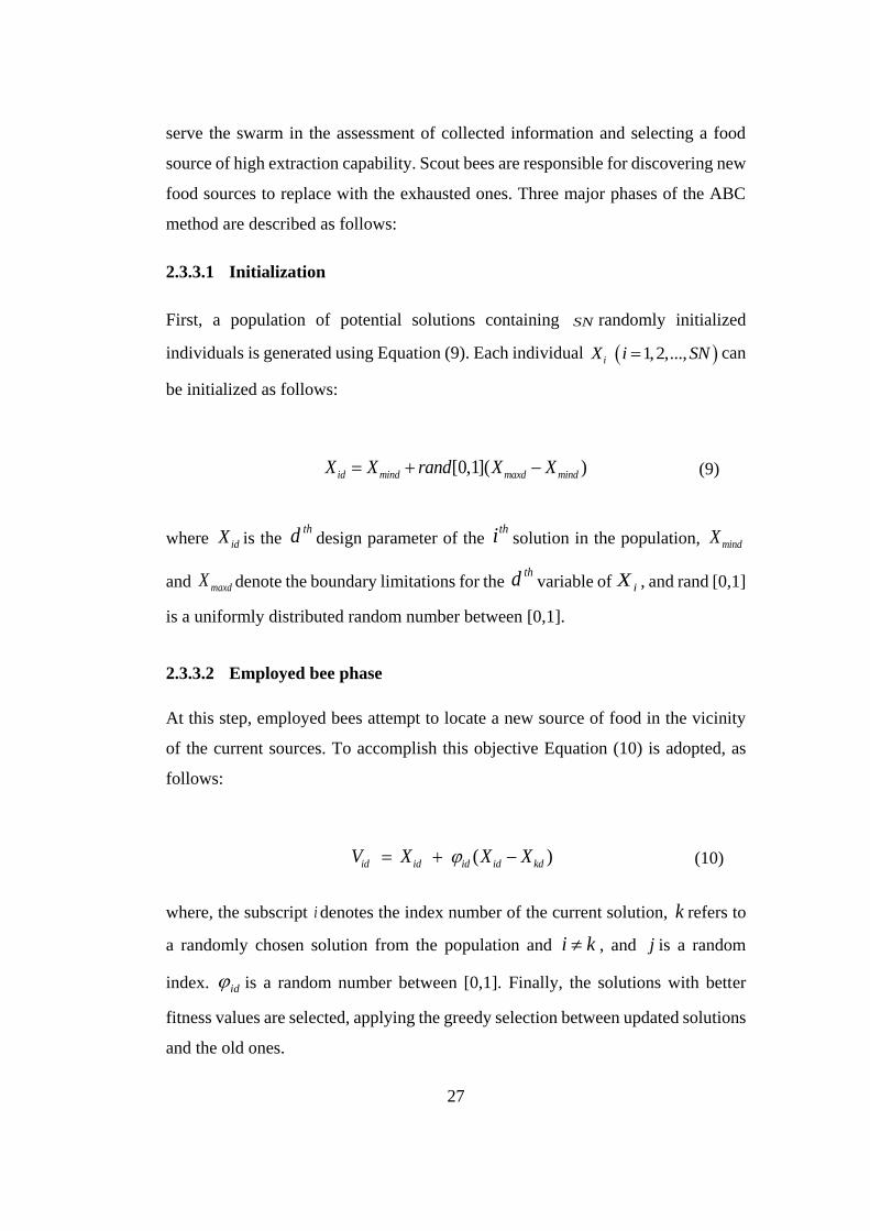
2.3.3.1 Initialization

First, a population of potential solutions containing SN randomly initialized

individuals is generated using Equation (9). Each individual 1,2,..., iX i SN can

be initialized as follows:

where idX is the thd design parameter of the

thi solution in the population, mindX

and maxdX denote the boundary limitations for the thd variable of iX , and rand [0,1]

is a uniformly distributed random number between [0,1].

2.3.3.2 Employed bee phase

At this step, employed bees attempt to locate a new source of food in the vicinity

of the current sources. To accomplish this objective Equation (10) is adopted, as

follows:

where, the subscript i denotes the index number of the current solution, k refers to

a randomly chosen solution from the population and i k , and j is a random

index. id is a random number between [0,1]. Finally, the solutions with better

fitness values are selected, applying the greedy selection between updated solutions

and the old ones.

0,1[ ]( )id mind maxd mindX X rand X X (9)

( ) id id id id kdV X X X (10)

28

2.3.3.3 Onlooker bee phase

Onlooker bees evaluate the information collected by employed bees to select a rich

source of food in order to search for better sources in their vicinity. This selection

is performed based on a probability which is proportional to the fitness value of the

solution (nectar amount of food source), as shown below:

where ifitness is the fitness value associated with the thi solution. Once an

appropriate candidate is selected, Equation (10) is then used to generate a new

candidate solution in the neighborhood. As in the previous phase, a greedy selection

between the updated solution and the old one is applied in order to select the

solution of the optimal value.

2.3.3.4 Scout bee phase

In ABC algorithm, a control parameter, namely limit, is defined in order to indicate

which of the solutions is abandoned (i.e. food sources exhausted). As a result, an

alternative food source is required to be located by a scout bee using Equation (9)

and replaced with the exhausted one.

1

( ) ii SN

n

n

fitnessprob G

fitness

(11)

29

CHAPTER 3

3.MAIN WORK

In this chapter, a complete description of the framework proposed for a reliable

slope stability evaluation with the application of optimization techniques is

provided. This procedure embraces three major steps, which include (1) generating

a number of trial slip surfaces, (2) evaluating safety factors corresponding to the

generated surfaces and lastly, (3) looking for the most critical failure surface

possessing the minimum safety factor. Following the procedure explained in the

first step, several non-circular failure surfaces composed of a predefined number of

slices can be generated. The value of safety factor is then required to be calculated

for each trial surface. Finally, in the third step, the optimization technique intends

to locate much critical surfaces within the slope, through making admissible

changes in the initial geometry of the surfaces. Detailed information about each step

is given in the following subsections.

3.1 Trial Slip Surface Generation Method

Initial trial surfaces can have either circular or non-circular geometry. A number of

slope stability studies have demonstrated that circular failure surfaces can be

successfully used where the case of study consists of a homogeneous soil layer;

however, the stability of slopes with multi-layered soil profile can be more precisely

evaluated through generating non-circular trial failure surfaces within the analysis

(Zolfaghari et al., 2005). Various methods have so far been implemented in the

literature for generating trial slip surfaces, and as noted by Cheng et al. (2008) the

results obtained in the analysis is highly dependent on the slip surface generation

method, and therefore different outcomes may be expected for the same slope in

this regard.

30

Amongst the methods proposed for generating trial slip surfaces to date, the method

recommended in the study by Cheng et al. (2008) is taken as the base for the

procedure followed in this study, through which admissible slip surfaces, i.e.

concave upward surface, can be formed as further outlined below. An example of

the generated surfaces is represented in Figure 8. The function g(x) indicates the

ground surface and h(x) marks the boundary separating different soil layers in the

slope. The n-slice nonlinear slip surface T is readily formed by connecting 1n

vertices 1 2 1( , ,..., )nV V V specified by the coordinates 1 1 2 2 1 1( , ), ( , ),..., ( , )n nx y x y x y .

The following steps are followed to generate a valid trial slip surface:

Initially, the x-coordinates of the start and endpoint of the surface along with

the inclination of the first 1( ) and last 1( )n slices are randomly determined

within their respective pre-defined ranges. Using the ground surface

function g(x), corresponding vertical coordinates can then be specified.

Care is required when defining the boundary limitations of the 1( ) and

1( )n in order to generate admissible surfaces.

Two lines are drawn through two end points of the surface with the specified

angles and the intersection point, i.e.V , is determined.

Equation (12) and (13) are employed to determine the coordinates of two

new vertices, i.e. second vertex 2V and a temporary vertex 7V .

where r is a randomly generated number between -0.5 and 0.5.

Subsequent points corresponding to the third and fourth vertices, 3V and

4V respectively, are placed at two neighboring line segments of the largest

2 1 2 1( )(0.5 ( 0.5,0.5))nx x x x r

(12)

2 1 2 1 1( ) tan( )y y x x (13)

31

horizontal lengths using equations similar to those of the previous step. This

procedure is followed in order to indicate the coordinates of all vertices

which simply constitute a trial surface of n slices described by the vector

1 1 5 2( , , , , ,..., )end end nV x x . The slip surface generation procedure is

then followed by safety factor evaluation of the respective surfaces, which

is further explained in the succeeding section.

Figure 8- Geometric Description of the Surface Generation Method

3.2 Calculation of Factor of Safety

As outlined in the previous chapter, several limit equilibrium methods that vary

depending on the inter-slice forces assumptions are introduced thus far, within them

the M-P method (Morgenstern & Price, 1965) in which all the equilibrium

conditions are perfectly met, has been exhaustively used in various studies in the

literature. This method, however, suffers from the difficulty to suggest appropriate

equations for the factor of safety and the scaling factor due to the non-linearity of

the force and moment equilibrium equations.

To overcome these difficulties, in this study a reformulated Morgenstern-Price

method is adopted for the slope stability analysis, which is developed by Zhu et al.

32

(2005). The changes made in this improved technique contributes to its simplicity

and facilitates the implementation of this algorithm into a computer program (D. Y.

Zhu et al., 2005).

As proposed in the original M-P method, the ratio of the normal forces over shear

inter-slice forces is calculated as follows:

where T and E refer to the inter-slice shear and normal forces, respectively. In

addition, f(x) in this equation is a prescribed function that may be in the form of a

constant, a trapezoidal, a half-sine or a user-defined function. λ is a scaling factor

that is to be determined when calculating the factor of safety.

Prior to the evaluation of the safety factor, the soil mas above the failure surface,

like other methods of slices, is divided into a number of slices which is then

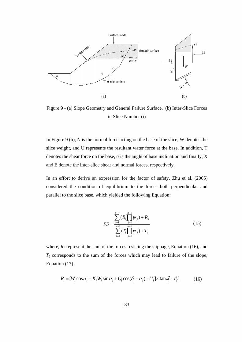
followed by determination of the forces imposed on each individual slice. Figure 9

below illustrates the geometry of a simple slope along with the inter-slice forces on

a representative slice. The symbols ℎ𝑖, 𝑏𝑖 and 𝛼𝑖 denote the slice height, slice width

and inclination of the slice base, respectively. Furthermore, 𝑊𝑖 denotes weight of

the slice, 𝐾𝑐 refers to seismic coefficient in the horizontal direction, 𝑤𝑖 is the

inclination of the external loading 𝑄𝑖 . Resultant pore water force is represented by

𝑈𝑖 , while 𝑢𝑖 denotes the mean water pressure. In addition, 𝑁′𝑖 corresponds to the

effective normal force on the slice base, 𝑐𝑖 is the effective cohesion, 𝜑′𝑖 is the

effective internal friction angle, 𝐹𝑠 is the safety factor and 𝑆𝑖 represents the slice

base mobilized shear resistance. 𝐸𝑖 and 𝐸𝑖−1are the normal inter-slice forces exerted

on the slice, while 𝑍𝑖 and 𝑍𝑖−1 denote the distances from the bottom of the slice to

the point of application of the corresponding normal inter-slice forces.

( ). .T f x E (14)

33

(a) (b)

Figure 9 - (a) Slope Geometry and General Failure Surface, (b) Inter-Slice Forces

in Slice Number (i)

In Figure 9 (b), N is the normal force acting on the base of the slice, W denotes the

slice weight, and U represents the resultant water force at the base. In addition, T

denotes the shear force on the base, α is the angle of base inclination and finally, X

and E denote the inter-slice shear and normal forces, respectively.

In an effort to derive an expression for the factor of safety, Zhu et al. (2005)

considered the condition of equilibrium to the forces both perpendicular and

parallel to the slice base, which yielded the following Equation:

where, 𝑅𝑖 represent the sum of the forces resisting the slippage, Equation (16), and

𝑇𝑖 corresponds to the sum of the forces which may lead to failure of the slope,

Equation (17).

[ cos sin cos( ) ] tani i i h i i i i i i i i iR W K W Q U c l (16)

11

1 1

11

1 1

( )

( )

nn

i j n

i j

nn

i j n

i j

R R

FS

T T

(15)

34

[ sin cos sin( )i i i h i i i i iT W K W Q (17)

1 1 1[i i i i i s i iE E F T R (18)

(sin cos ) tan (cos sin )i i i i i i i i sf f F (19)

1 1 1 1[(sin cos ) tan (cos sin ) ] /i i i i i i i i s if f F

(20)

where parameter E refers to the inter-slice forces on the vertical sides of slices.

From the Equation (15), it can be inferred that an iterative procedure needs to be

followed so as to determine the factor of safety since the equation has the FS on

both sides.

Likewise, resolving moments about a point in the center of the slice, an explicit

Equation is developed for the scaling factor:

where parameter E refers to the inter-slice forces on the vertical sides of slices

which is determined as follows:

It is important to note that at the lower and upper bounds of the slope, 𝐸0 and 𝐸𝑛

respectively, the inter-slice forces are neglected, (𝐸0=𝐸𝑛=0).

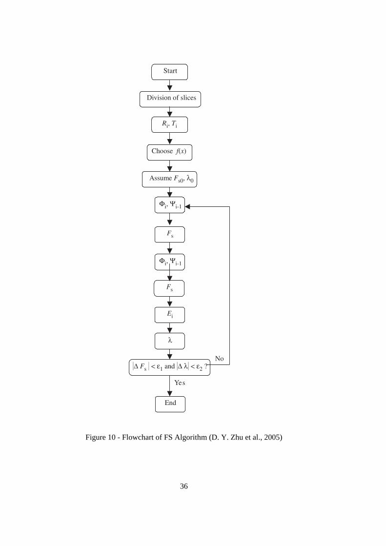
The complete iterative procedure for the factor of safety calculation is illustrated in

Figure 10. As shown, once the value of 𝑅𝑖 and 𝑇𝑖 are determined, it is then required

1

1

1 1

1

[ ( ) tan 2 sin ]

[ ( )]

n

i i i i h i i i i i

i

n

i i i i i

i

b E E K W h Q h

b f E f E

(21)

1 1 1[(sin cos ) tan (cos sin ) ]

)(sin cos ) tan (cos sin )

i i i i i i i i i ii

i i i i i i i

f f FS E FST RE

f f FS

(22)

35

to define the type of inter-slice function f(x), a constant function (f(x) = 1) is adopted

in this study, as well as to initialize the factor of safety and the scaling factor. Zhu

et al. (2005) proposed initial values of 1 and 0 for 𝐹𝑠 and 𝜆, respectively. Next step

is to calculate the value of FS using Equation (15), followed by evaluation of 𝜆 for

which the Equation (21) is utilized. These updated values are then substituted for

the prescribed FS and 𝜆 values, and an iterative procedure is continued until the

absolute differences in FS value as well as the value of 𝜆 in successive iterations is

less than predefined parameters 𝜀1 and 𝜀2; a value of 0.0001 is proposed for both

of these limits.

36

Figure 10 - Flowchart of FS Algorithm (D. Y. Zhu et al., 2005)

37

3.3 Optimization Methods

As has been pointed out in the previous sections, the main goal of a slope stability

assessment is to evaluate the minimum safety factor corresponding to a geological

surface along which the soil is more prone to slide down the slope. This objective

can be reliably achieved by an optimization process formulated as follows:

where V is a trial solution vector containing control variables of the sliding surface

and ( )FS V is the safety factor of the generated failure surface. minix and maxix denote

the boundary limitations of the starting and end points of the surface and nVar

indicates the number of control variables within the solution vector. The

minimization procedure starts with the construction of a population of randomly

generated solution vectors followed by evaluation of the corresponding objective

function values, factors of safety, by using the method proposed in the previous

section. The search for solutions with huge potential for further improvement in the

objective value is continued through updating the variables of solution vectors over

the successive iterations. Once the predefined termination criteria are met, the

optimum objective value of the problem, pertaining to the best candidate solution

is finally achieved. Detailed information about the implementation process of the

proposed optimization methods is given in the following subsections.

Find 1 1 5 2( , , , , ,..., )end end nV x x (23)

To minimize ( )FS V (24)

Subjected to min max , 1,i i ix x x i nVar (25)

0.5 0.5, 5,6,...,j j nVar (26)

38

3.3.1 Improved harmony search algorithm (LHS)

Review of the available evidence on the application of the harmony search method

establishes its limitations in exploring the optimum solution, particularly in the case

of complicated optimization problems and demonstrates the need for further

refinements in its algorithm. In this regard, Ouyang et al. (2017) proposed an

improved harmony search algorithm (LHS) which enhances the ability of HS

algorithm both in exploring the search space thoroughly in order to discover a

region of better candidate solutions, along with locating new promising solutions

in the neighborhood of the current optimum solution. Three major alteration to the

harmony search algorithm is made which includes the incorporation of (1) local

opposition-based learning, (2) self-adaptation global pitch adjusting, and (3)

competition-selection strategies into the original HS method. The implementation

procedure of LHS is outlined and a brief overview of the selection of appropriate

parameters for this method is given, as follows:

3.3.1.1 Definition of the Algorithm

In opposition-based learning scheme, a candidate solution and its opposing solution

are generated simultaneously in order to explore the search space more

comprehensively. Exploitation ability in harmony search method, however, is

mainly influenced by the pitch adjusting operation. Consequently, employing a self-

adapting pitch adjustment concept can improve the efficacy of the harmony search

method in problem solving. Adoption of the competition-selection approach helps

the algorithm update the existing harmony memory over the successive iterations.

The implementation procedure of the LHS is summarized as follows:

3.3.1.1.1 Initializing algorithm and problem parameters

In this step, harmony memory size (HMS), harmony memory consideration rate

(HMCR), the maximum dimension of candidate solutions D, lower and upper

bounds for the control variables and maximum generation number G, are required

to be specified.

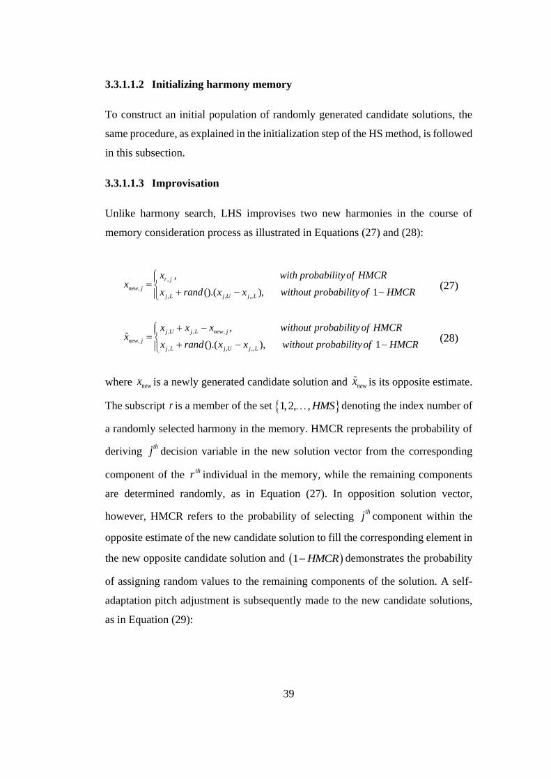
39

3.3.1.1.2 Initializing harmony memory

To construct an initial population of randomly generated candidate solutions, the

same procedure, as explained in the initialization step of the HS method, is followed

in this subsection.

3.3.1.1.3 Improvisation

Unlike harmony search, LHS improvises two new harmonies in the course of

memory consideration process as illustrated in Equations (27) and (28):

where newx is a newly generated candidate solution and newx is its opposite estimate.

The subscript r is a member of the set 1,2, , HMS denoting the index number of

a randomly selected harmony in the memory. HMCR represents the probability of

deriving thj decision variable in the new solution vector from the corresponding

component of the thr individual in the memory, while the remaining components

are determined randomly, as in Equation (27). In opposition solution vector,

however, HMCR refers to the probability of selecting thj component within the

opposite estimate of the new candidate solution to fill the corresponding element in

the new opposite candidate solution and 1 HMCR demonstrates the probability

of assigning random values to the remaining components of the solution. A self-

adaptation pitch adjustment is subsequently made to the new candidate solutions,

as in Equation (29):

,

, ,,

,

, ().( 1

,

),j L j U

r j

ne

j L

w j

x wi

x rand x x without pro

th

ba

probab

bility

ility of H

of HMC

M

R

CRx

(27)

, , ,

,

, , ,,().( ),

,

1j L j U j L

j U j L new j

new j

x x x without proba

x rand x x without probabi

bility

lity of HMCR

of HMCRx

(28)

40

where ,best jx and ,worst jx represent the index number of selected components within

the best and worst individuals in the memory, respectively. Incorporation of the

best and worst individuals helps the algorithm approach the global optimum over

the successive generations. The parameter represents a dynamic factor where its

value is dependent on the number of the current iteration along with the maximum

iterations number, as expressed in Equation (30):

where k denotes the current iteration’s number, and the maximum iterations

number is depicted with K .

3.3.1.1.4 Updating

In this step, fitness value for both the new solution and its opposite estimate is

compared and the better solution is substituted for the worst individual in the

population.

3.3.1.1.5 Termination

The procedure will be continued until the maximum number of iterations is reached

and the best solution will be reported. Figure 11 and Figure 12, illustrate the

implementation process of the proposed method.

.

, , ,

,

, , ,

( ),

( ),

r j best j r j

new j

r j worst j r j

x rand x x if randx

x rand x x otherwise

(29)

1 1.5 / , / 2

0.5, / 2 3 / 4

exp 14.53 14.04 / ,

k K k K

K k K

k K otherwise

(30)

41

3.3.1.2 Parameter Selection

Appropriate determination of the key parameters involved in any optimization

method requires an extensive research effort. In this regard, Ouyang et al. (2017)

carried out a number of investigations into the impacts of the values assigned to

HMS and HMCR on the performance of LHS; according to their study, selection

of a small value for HMS would yield much promising results while, in contrast, a

large value is recommended for the HMCR (HMCR > 0.90) for a better

performance.

In an effort to determine the appropriate parameter values in this study, slope

stability analysis using LHS method is repeated several times, with varied values

assumed for the HMS and the HMCR. Based on the results obtained, the selected

values for these parameters are as follows: HMCR= 0.99 and HMS = 40.

42

Figure 11 - Two main branches about the improvisation process (Ouyang et al.,

2017)

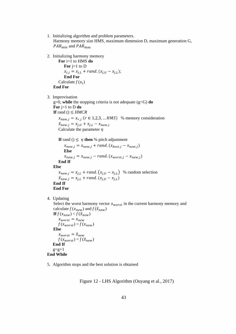
43

1. Initializing algorithm and problem parameters.

Harmony memory size HMS, maximum dimension D, maximum generation G,

𝑃𝐴𝑅min and 𝑃𝐴𝑅max

2. Initializing harmony memory

For i=1 to HMS do

For j=1 to D

𝑥𝑖,𝑗 = 𝑥𝑗,𝐿 + 𝑟𝑎𝑛𝑑. (𝑥𝑗,𝑈 − 𝑥𝑗,𝐿);

End For

Calculate f (𝑥𝑖)

End For

3. Improvisation

g=0, while the stopping criteria is not adequate (g<G) do

For j=1 to D do

If rand () ≤ HMCR

𝑥𝑛𝑒𝑤,𝑗 = 𝑥𝑟,𝑗 (𝑟 ∈ 1,2,3, … 𝐻𝑀𝑆) % memory consideration

�̃�𝑛𝑒𝑤,𝑗 = 𝑥𝑗,𝑈 + 𝑥𝑗,𝐿 − 𝑥𝑛𝑒𝑤,𝑗

Calculate the parameter 𝜂

If rand () ≤ 𝜂 then % pitch adjustment

𝑥𝑛𝑒𝑤,𝑗 = 𝑥𝑛𝑒𝑤,𝑗 + 𝑟𝑎𝑛𝑑. (𝑥𝑏𝑒𝑠𝑡,𝑗 − 𝑥𝑛𝑒𝑤,𝑗)

Else

𝑥𝑛𝑒𝑤,𝑗 = 𝑥𝑛𝑒𝑤,𝑗 − 𝑟𝑎𝑛𝑑. (𝑥𝑤𝑜𝑟𝑠𝑡,𝑗 − 𝑥𝑛𝑒𝑤,𝑗)

End If

Else

𝑥𝑛𝑒𝑤,𝑗 = 𝑥𝑗,𝐿 + 𝑟𝑎𝑛𝑑. (𝑥𝑗,𝑈 − 𝑥𝑗,𝐿) % random selection

�̃�𝑛𝑒𝑤,𝑗 = 𝑥𝑗,𝐿 + 𝑟𝑎𝑛𝑑. (𝑥𝑗,𝑈 − 𝑥𝑗,𝐿)

End If

End For

4. Updating

Select the worst harmony vector 𝑥𝑤𝑜𝑟𝑠𝑡 in the current harmony memory and

calculate f (𝑥𝑛𝑒𝑤) and f (�̃�𝑛𝑒𝑤)

If f (𝑥𝑛𝑒𝑤) < f (�̃�𝑛𝑒𝑤)

𝑥𝑤𝑜𝑟𝑠𝑡 = 𝑥𝑛𝑒𝑤

f (𝑥𝑤𝑜𝑟𝑠𝑡) = f (𝑥𝑛𝑒𝑤)

Else

𝑥𝑤𝑜𝑟𝑠𝑡 = �̃�𝑛𝑒𝑤

f (𝑥𝑤𝑜𝑟𝑠𝑡) = f (�̃�𝑛𝑒𝑤)

End If

g=g+1

End While

5. Algorithm stops and the best solution is obtained

Figure 12 - LHS Algorithm (Ouyang et al., 2017)

44

3.3.2 Grasshopper optimization algorithm (GOA)

Grasshopper optimization algorithm (GOA) is a recent nature-inspired stochastic

optimization method proposed by Saremi et al. (2017). Mathematical theorem of

the GOA is thoroughly formed on the basis of the natural behavior of grasshopper

swarm in foraging the farms for adequate sources of food. Each grasshopper in this

method relocates from its current position according to the location of the best

forager, a grasshopper possessing the optimal objective value, and remaining

agents’ position. Simulation of the social interaction, i.e. repulsion and attraction

forces, between the grasshoppers which is balanced with a decreasing coefficient

help GOA thoroughly explore the design space in order to discover the most

adequate food source, i.e. the optimum value of the objective function. Successful

application of the proposed method on several test functions of various

complexities as well as design optimization of multiple real problems has

demonstrated the accuracy and applicability of GOA in obtaining the optimum

solutions. The implementation process of the GOA is summarized as follows:


The initial position of N number of potential solutions (grasshoppers) in the search

space is randomly determined prior to the formation of the foraging swarm. Control

parameters of GOA, including maxC , minC as well as the number of maximum

iterations are also required to be specified in this phase. Objective value of each

candidate solution is then evaluated and the one owning the optimum objective

value – best candidate solution – is subsequently determined. A successful

optimization process, however, requires the entire search space to be

comprehensively explored. In this regard, Equation (31) is introduced in GOA

which helps the grasshoppers update their current position, and thus discover new

regions in the neighborhood. It also can be inferred from the Equation (31) that in

addition to the position of both the current grasshopper and the best individual thus

far, the remaining members of the swarm play a considerable role in updating the

current positions.

45

where d

iX indicates the updated position of the thi individual in the thd dimension,

N refers to the number of individuals, dlb and dub define the boundary limits in

dimension d , d d

j ix x represents the distance separating the individuals i and j. In

addition, ( )j i ij

x x d indicates a vector of magnitude 1, from individual i to

individual j. dT is the th

d component of the best candidate solution in the swarm, and

subscripts i and j refer to the thi and

thj grasshopper, respectively. In Equation (31),

c is a coefficient balancing the attraction and repulsion forces between the search

agents, which contributes to the improvement of the results through guiding the

search agents towards the best solution within the swarm. Value of the coefficient

c varies over the successive iterations and it can be determined by using Equation

(32) as follows:

where 𝑐𝑚𝑎𝑥 and 𝑐𝑚𝑖𝑛 refer to the boundary limitations for the coefficient c,

parameter l denotes the current iteration, and L is the maximum iterations number.

In addition, s in the Equation (31) is a function which measures the interactive

forces between the grasshoppers. Equation (33) is proposed for this purpose, as

follows:

where parameter f denotes the attraction intensity and l refers to the scale of the

attractive length.

1 2

Nj id d dd d

i j i d

j ijj i

x xub lbX c c s x x T

d

(31)

max minmax

c cc c l

L

(32)

( )r

rls r f e e

(33)

46

The search for regions with huge potential for further improvement in the objective

value is continued through updating the position of search agents over the

successive iterations. Once the predefined termination criteria are met, the optimum

fitness value of the problem, corresponding to the best target is finally achieved.

Figure 13, illustrates the pseudo codes of the proposed method.


In an effort to determine appropriate values for the key parameters of the GOA,

Saremi et al. (2017) carried out a number of investigations into the impacts of the

values assigned to f and l on the performance of function s. According to their study,

the function s would yield much promising results when assuming l=1.5 and f=0.5.

In addition, as for the parameters 𝑐𝑚𝑎𝑥and 𝑐𝑚𝑖𝑛, the values 1 and 0.00001 are

recommended, respectively,


stability analysis using GOA method is repeated several times, with varied values

assumed for the boundary limitations of the parameter c – 𝑐𝑚𝑎𝑥 and 𝑐𝑚𝑎𝑥. Based

on the results obtained, the selected values for these parameters are as follows:

𝑐𝑚𝑎𝑥= 2 and 𝑐𝑚𝑖𝑛 = 0.001. It is worth mentioning that the values proposed in the

original study are used for the parameters l and f.

47

3.3.3 Hybrid Artificial Bee Colony with Differential Evolution (HABCDE)

Recent studies have consistently shown that basic ABC, as mentioned earlier, lacks

the ability to exploit better solutions as it lacks the capability of taking advantage

of the information collected by the forager bees swarm. So far, however, there has

been made considerable attempts to get around the above-mentioned drawbacks.

Jadon et al. (2017) hybridized Artificial Bee Colony and Differential Evolution

methods to develop a new algorithm, namely HABCDE, which benefits both from

the advantages of ABC, such as (1) straightforward implementation and (2) few

parameter adjustment requirements, and from the fast-converging feature of the

differential evolution algorithm. Various modifications are carried out on each

phase of ABC to enhance its efficiency and convergence speed as well as to obtain

results of high accuracy. In HABCDE, employed bees utilize an updated equation

Initialize the swarm 𝑋𝑖, (i= 1,2,…,n)

Initialize 𝑐𝑚𝑎𝑥, 𝑐𝑚𝑖𝑛 and maximum number of iterations

Calculate the fitness of each search agent

T= the best search agent

While (l < Max number of iterations)

Update c using Equation (32)

For each search agent

Normalize the distances between grassoppers in [1,4]

Update the position of the current search agent by the Equation (31)

Bring the current search agent back if it goes outside the boundaries

End for

Update T if there is a better solution

l= l+1

End while

Return T

Figure 13 - GOA Algorithm (Saremi et al., 2017)

48

while exploring food sources. Besides, onlooker bees in HABCDE exploit the

current solutions by the means of DE’s evolutionary operations, and the entire scout

bees in this method are required to look for new alternative food sources to replace

exhausted ones.


In the following subsections, the implementation process of the proposed HABCDE

method is outlined in three phases. Also, a brief overview of the parameter selection

for this method is provided, as follows:

3.3.3.1.1 Initialization

First, a population of potential solutions containing SN randomly initialized

individuals is generated using Equation (34). Each individual ( 1,2,..., )iX i SN

can be generated as follows:

where idX is the thd design parameter of the thi solution in the population, min dX

and max dX denote the boundary limitations for the thd variable of iX , and rand [0,1]

is a random number selected from a uniform distribution between [0,1].

3.3.3.1.2 Employed bee phase

At this step, employed bees attempt to locate a new source of food surrounding the

current sources. To accomplish this objective, a search equation similar to the one

proposed in gbest-guided ABC (G. Zhu & Kwong, 2010) is adopted, which

contributes to the improvement in exploitation ability of the employed method

through the incorporation of the position of the best candidate solution into

Equation (35), as follows:

min max min rand[0.1] ( )id d d dX X X X (34)

49

where, the subscript i indicates the index number of the current solution, k refers to

a solution selected randomly from the population and i≠ 𝑘, and j is a randomly

selected index. 𝜑𝑖𝑑 is a random number in the interval [0,1], 𝑦𝑑 is the 𝑑𝑡ℎ variable

within the best individual. Ψ is a random number in the interval 0, C and C is a

positive user-defined constant. Finally, the solutions with better fitness values are

selected by using the greedy selection mechanism between updated solutions and

the old ones.

3.3.3.1.3 Onlooker bee phase

Onlooker bees evaluate the information collected by employed bees to serve the

purpose of selecting rich sources of food in an effort to search for better sources in

their vicinity. This selection is performed on merit based on a probability iprob ,

which is proportional to the solution’s fitness value, as shown below:

where ifitness is the calculated fitness value associated with the 𝑖𝑡ℎ solution. To

generate new candidate solutions, DE’s evolutionary operations, i.e. mutation,

crossover, and selection, are utilized. This process starts with generating a mutated

vector according to the best food source position as well as the position of two other

sources which are selected randomly from the population as presented in Equation

(3) in the previous chapter. Following this, a crossover operation, as in Equation

(4), is applied and current solution’s design variables are merged with those of

mutated vector to produce a trial vector. Finally, selection operator, Equation (5),

is applied in the last phase so as to determine the solution of the optimal value.

( ) ( )id id id id kd id d idv x x x y x (35)

(36) 0.9

( ) 0.1i

i

fitnessprob G

maxfit

50

3.3.3.1.4 Scout bee phase

Typically, available nutrients of the food sources get exhausted due to the continued

exploitation by the forager bees. A candidate solution in ABC is called abandoned

if its corresponding control parameter reaches a predefined value, namely limit,

after a number of successive iterations. In basic ABC, a scout bee identifies an

alternative source of food, by using Equation (34), to replace the exhausted one.

However, in the proposed method, all the exhausted solutions update their current

position to lead to an improvement in the exploration capability of HABCDE.

Consequently, the optimum solution for the problem can be discovered by

performing this three-step iterative procedure until a certain termination criterion is

met. Figure 14 and Figure 15, illustrate the implementation process of the proposed

method.


In an effort to determine the appropriate setting for the key parameters of the

HABCDE, Jadon et al. (2017) carried out a number of investigations into the

impacts of the values assigned to F and CR – key parameters of DE method – on

the performance of proposed method. According to their study, the method would

yield much promising results with the values F=0.7 and CR=0.6 assumed in the

analyses.


stability analysis using HABCDE method is repeated several times, with varied

values assumed for the parameters F and CR. Based on the results obtained, the

selected values for these parameters are as follows: F = 0.7 and CR = 0.9.

51

Figure 14 - HABCDE Algorithm (Jadon et al., 2017)

Initialize the swarm and control parameters;

While !Termination criteria do

Employed bee phase: generate neighborhood solutions for each solution in

the swarm using position update Equation (35)

Onlooker bees phase: generate neighborhood solutions for the solutions

selected based on their probabilities as follows:

for (each onlooker’s solution x𝑖) do

if (U (0, 1) < prob𝑖) then

Apply mutation (as in Equation(3)) to generate the trial solution u𝑖

Apply binomial crossover (as in Equation(4)) to generate an offspring x′𝑖

if (f (x′𝑖) is better than f (x𝑖)) then

x𝑖 =x′𝑖

end if

end if

end for

Scout bee phase: randomly reinitialize all the exhausted solutions in the

search space.

end while

Output the best solution.

52

Figure 15 - Flowchart for HABCDE Algorithm (Jadon et al., 2017)

Initialize solutions

Calculate Fitness

Employed bee phase

(Determine neighbor of the solutions using Eq. 35)

Onlooker bee phase

( Select solutions based on probabili ty using Eq. 36 )

Apply DE/best/1/bin proces s:

2. generate new solution using crossover operator (Eq. 4)

3. select new or old solution base d on fitness using selection operator (Eq. 5)

Memorize the best solution

(produce new solutions in pla ce of all exhausted solutions using Eq. 34 )

Final solutions

Yes

NoIs termination

criteria

satisfied ?

Calculate Fitness

1. generate trial solution using mutation operation (Eq. 3)

Scout bee phase:

53

CHAPTER 4

4.CASE STUDIES

In this section capability and efficacy of the proposed methods in determination of

the expected failure surface and the relating factor of safety are thoroughly revealed.

In this regard, four case studies of varying computational complexity are

considered. Selected numerical examples consist of a set of three complex layered

slopes of diverse geometries and a simple homogeneous slope problem, subjected

to different external loading conditions. Furthermore, computer codes developed in

MATLAB software are used for the implementation of the optimization methods in

the analyses. The analyses are performed with 40 randomly initialized individuals

and 3000 generations. Each of the case studies is solved 30 times to reduce the

possible statistical errors which may arise in association with the stochastic

behavior of the optimization techniques. Also, in this study, the slice number is set

equal to 20 in all the case studies.

Analyses results in this study are compared with those obtained in previous studies

carried out by different researchers and summarized in tables. A comprehensive

comparison of the results necessitates the use of identical assumptions and analysis

methods for the same slope problem. Available results in the literature are, however,

obtained by using different limit equilibrium method. This consequently might

adversely affect the reliability of the comparison; however, it is believed that

adequate comparisons of different metaheuristic methods can be made in terms of

their accuracy as well as the overall performance. In the following sections,

available information about the geometry of the case studies along with the

characteristic of the soil in situ is provided in details.

54

4.1 Case study 1

As the first test case, a homogeneous earth slope with a simple geometry as

presented in Figure 16 is considered. Information about the soil parameters of this

slope is, for effective cohesion c =9.8 kN 𝑚3⁄ , unit weight γ =17.64 kN 𝑚3⁄ ,

residual friction angle φ =10° and the water table is not observed within the slope.

Figure 16 - Slope geometry—Example 1

Various optimization schemes are used to solve this problem, where the comparison

of the results allows researchers to benchmark the performance of one optimization

technique against other methods. Classical optimization methods such as the

Davidon-Fletcher-Powell (DFP) method, the Broyden-Fletcher-Goldfarb-Shanno

(BFGS) method, the Powell method and the simplex method, integrated with the

Morgenstern-Price method (assuming interslice function, f(x)=1) are used by

Yamagami and Ueta (1988) in their study to locate the noncircular failure surface

in this problem. Additionally, Greco (1996) adopted the Mont-Carlo and pattern

search methods to determine the minimum safety factor. This problem has also been

55

studied with several metaheuristic algorithms including, genetic algorithms as in

Sun et al. (2008), harmony search and particle swarm techniques in Cheng et al.

(2007; 2008), and ant colony optimization algorithm in the work by Kahatadeniya

et al. (2009). Table 2 provides an overview of the optimum results obtained in the

literature by applying different methods on this problem. It is worth mentioning that

NOF in the table below refers to the overall number of evaluations performed

during the analyses.

Table 2 - Result Comparison – Example 1

Study Method Optimization

Method FS NOF

Yamagami

(1988) Spencer BFGS,DFP,Powell 1.338 NA

Greco

(1996) Spencer Monte Carlo 1.327-1.333 NA

Cheng et al.

(2008) MP Modified HS 1.3379 10568

Cheng et al.

(2006) Spencer PSO 1.3249 54022

Cheng et al.

(2007) Spencer Modified PSO 1.3273 20021

Sun et al.

(2008) Spencer GA

1.324 (line)

NA

1.321(spline)

Kahatadeniya et al

(2009) MP ACO 1.311 NA

Khajezadeh et al.

(2012) MP

PSO 1.321 NA

MPSO 1.308 NA

Kashani et al.

(2014) MP ICA 1.3206 NA

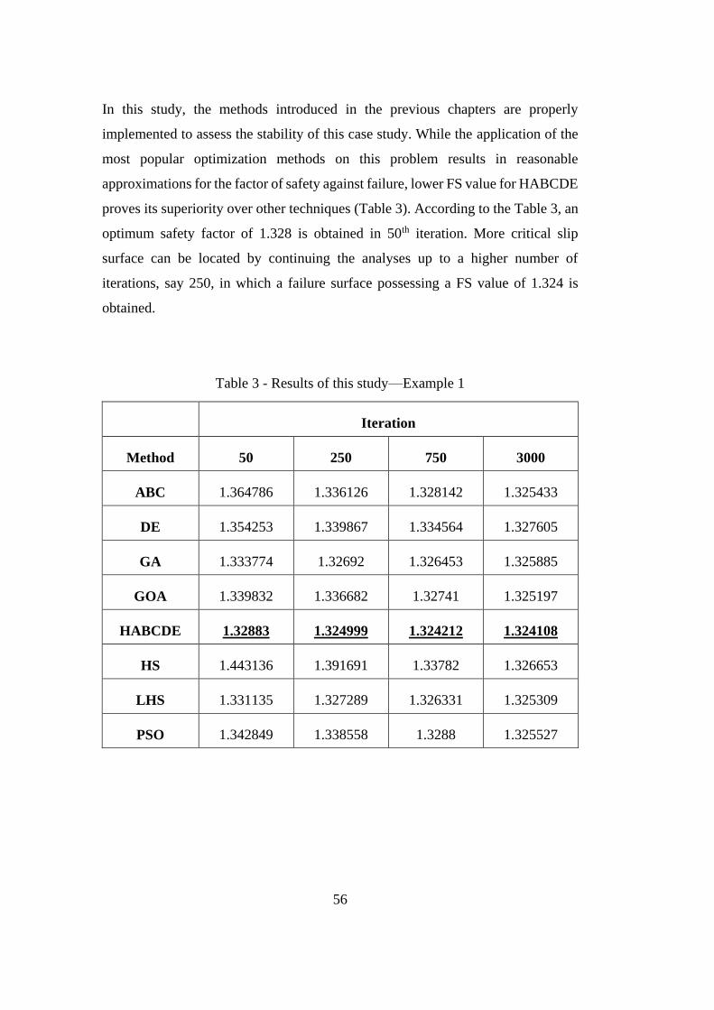
56

In this study, the methods introduced in the previous chapters are properly

implemented to assess the stability of this case study. While the application of the

most popular optimization methods on this problem results in reasonable

approximations for the factor of safety against failure, lower FS value for HABCDE

proves its superiority over other techniques (Table 3). According to the Table 3, an

optimum safety factor of 1.328 is obtained in 50th iteration. More critical slip

surface can be located by continuing the analyses up to a higher number of

iterations, say 250, in which a failure surface possessing a FS value of 1.324 is

obtained.

Table 3 - Results of this study—Example 1

Iteration

Method 50 250 750 3000

ABC 1.364786 1.336126 1.328142 1.325433

DE 1.354253 1.339867 1.334564 1.327605

GA 1.333774 1.32692 1.326453 1.325885

GOA 1.339832 1.336682 1.32741 1.325197

HABCDE 1.32883 1.324999 1.324212 1.324108

HS 1.443136 1.391691 1.33782 1.326653

LHS 1.331135 1.327289 1.326331 1.325309

PSO 1.342849 1.338558 1.3288 1.325527

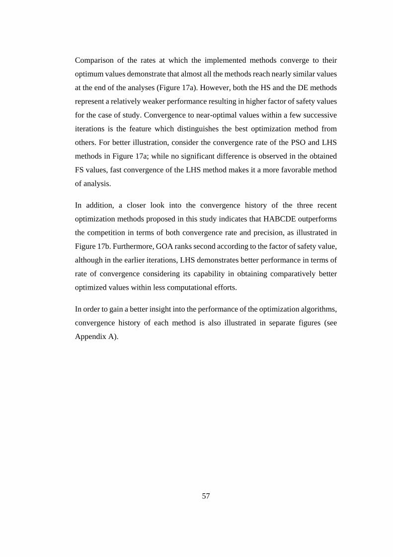
57

Comparison of the rates at which the implemented methods converge to their

optimum values demonstrate that almost all the methods reach nearly similar values

at the end of the analyses (Figure 17a). However, both the HS and the DE methods

represent a relatively weaker performance resulting in higher factor of safety values

for the case of study. Convergence to near-optimal values within a few successive

iterations is the feature which distinguishes the best optimization method from

others. For better illustration, consider the convergence rate of the PSO and LHS

methods in Figure 17a; while no significant difference is observed in the obtained

FS values, fast convergence of the LHS method makes it a more favorable method

of analysis.

In addition, a closer look into the convergence history of the three recent

optimization methods proposed in this study indicates that HABCDE outperforms

the competition in terms of both convergence rate and precision, as illustrated in

Figure 17b. Furthermore, GOA ranks second according to the factor of safety value,

although in the earlier iterations, LHS demonstrates better performance in terms of

rate of convergence considering its capability in obtaining comparatively better

optimized values within less computational efforts.

In order to gain a better insight into the performance of the optimization algorithms,

convergence history of each method is also illustrated in separate figures (see

Appendix A).

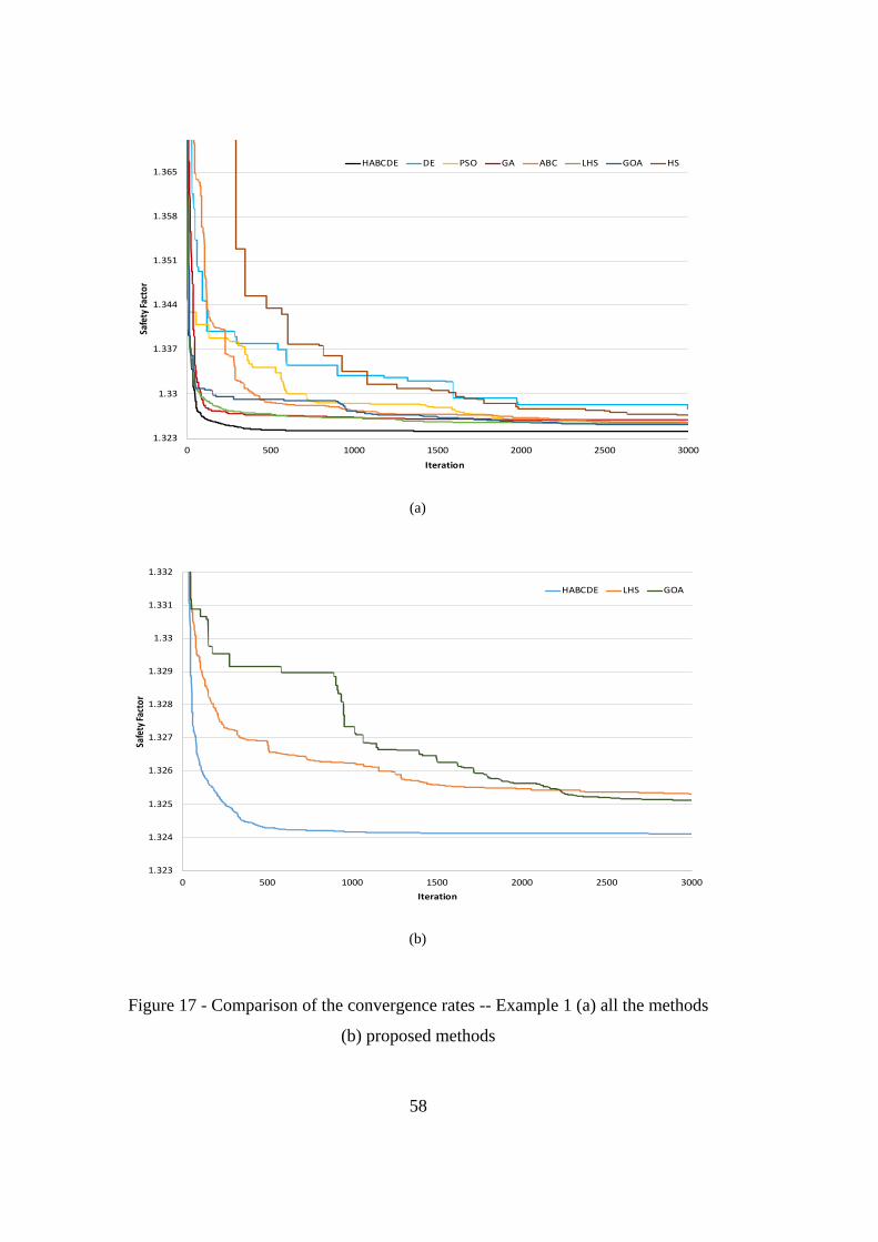
58


(b) proposed methods

(a)

(b)

1.323

1.33

1.337

1.344

1.351

1.358

1.365

0 500 1000 1500 2000 2500 3000

Safe

ty F

acto

r

Iteration

HABCDE DE PSO GA ABC LHS GOA HS

1.323

1.324

1.325

1.326

1.327

1.328

1.329

1.33

1.331

1.332

0 500 1000 1500 2000 2500 3000

Safe

ty F

acto

r

Iteration

HABCDE LHS GOA

59

Furthermore, in Figure 18, the critical slip surfaces associated with the implemented

methods are displayed graphically. From this figure, the sensitivity of the safety

factor to slight changes in the location of the failure surface can be readily inferred.

Figure 18 - Critical Slip Surfaces -- Example 1

4.2 Case study 2

In the second case, a non-homogeneous earth slope comprising four layers of

different soil properties which is first proposed by Zolfaghari et al. (2005), is

considered. Figure 19 illustrates the slope geometry and Table 4 indicates the soil

parameters of each layer, independently. Presence of the low-resistant soil layer in

the slope profile makes it a challenging optimization problem attributable to various

local optimum points existing in the search space, and consequently, determination

of the expected slip surface entirely depends on the ability of the optimization

techniques in evading these local minima.

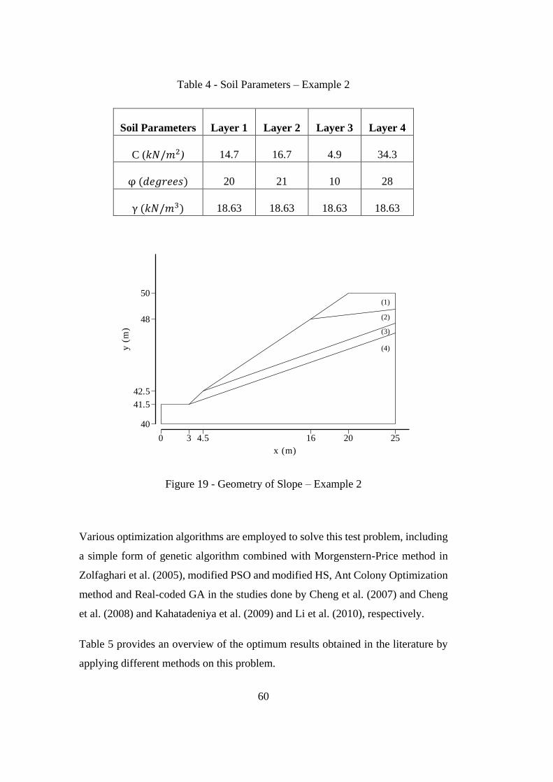
60

Table 4 - Soil Parameters – Example 2

Soil Parameters Layer 1 Layer 2 Layer 3 Layer 4

C (𝑘𝑁/𝑚2) 14.7 16.7 4.9 34.3

φ (𝑑𝑒𝑔𝑟𝑒𝑒𝑠) 20 21 10 28

γ (𝑘𝑁/𝑚3) 18.63 18.63 18.63 18.63

Figure 19 - Geometry of Slope – Example 2

Various optimization algorithms are employed to solve this test problem, including

a simple form of genetic algorithm combined with Morgenstern-Price method in

Zolfaghari et al. (2005), modified PSO and modified HS, Ant Colony Optimization

method and Real-coded GA in the studies done by Cheng et al. (2007) and Cheng

et al. (2008) and Kahatadeniya et al. (2009) and Li et al. (2010), respectively.

Table 5 provides an overview of the optimum results obtained in the literature by

applying different methods on this problem.

0 3 4.5 16 20 25

40

41.5

42.5

48

50

x (m)

y(m

)

(1)

(2)

(3)

(4)

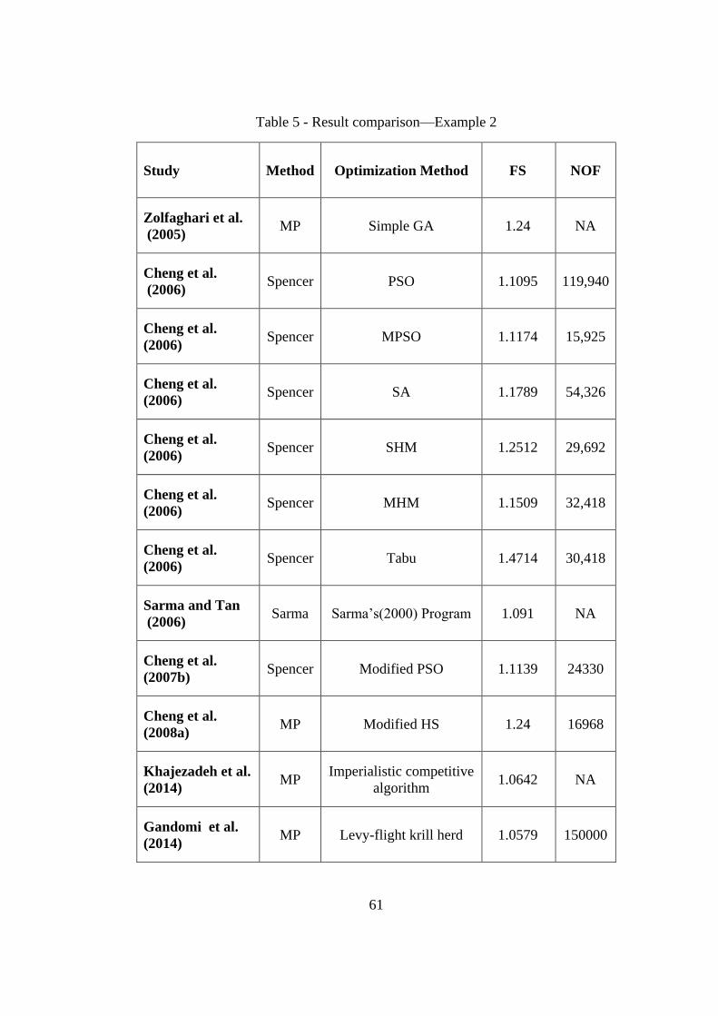
61

Table 5 - Result comparison—Example 2

Study Method Optimization Method FS NOF

Zolfaghari et al.

(2005) MP Simple GA 1.24 NA

Cheng et al.

(2006) Spencer PSO 1.1095 119,940

Cheng et al.

(2006) Spencer MPSO 1.1174 15,925

Cheng et al.

(2006) Spencer SA 1.1789 54,326

Cheng et al.

(2006) Spencer SHM 1.2512 29,692

Cheng et al.

(2006) Spencer MHM 1.1509 32,418

Cheng et al.

(2006) Spencer Tabu 1.4714 30,418

Sarma and Tan

(2006) Sarma Sarma’s(2000) Program 1.091 NA

Cheng et al.

(2007b) Spencer Modified PSO 1.1139 24330

Cheng et al.

(2008a) MP Modified HS 1.24 16968

Khajezadeh et al.

(2014) MP

Imperialistic competitive

algorithm 1.0642 NA

Gandomi et al.

(2014) MP Levy-flight krill herd 1.0579 150000

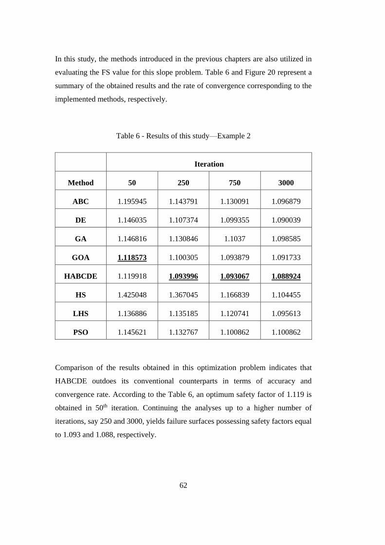
62

In this study, the methods introduced in the previous chapters are also utilized in

evaluating the FS value for this slope problem. Table 6 and Figure 20 represent a

summary of the obtained results and the rate of convergence corresponding to the

implemented methods, respectively.


Iteration

Method 50 250 750 3000

ABC 1.195945 1.143791 1.130091 1.096879

DE 1.146035 1.107374 1.099355 1.090039

GA 1.146816 1.130846 1.1037 1.098585

GOA 1.118573 1.100305 1.093879 1.091733

HABCDE 1.119918 1.093996 1.093067 1.088924

HS 1.425048 1.367045 1.166839 1.104455

LHS 1.136886 1.135185 1.120741 1.095613

PSO 1.145621 1.132767 1.100862 1.100862

Comparison of the results obtained in this optimization problem indicates that

HABCDE outdoes its conventional counterparts in terms of accuracy and

convergence rate. According to the Table 6, an optimum safety factor of 1.119 is

obtained in 50th iteration. Continuing the analyses up to a higher number of

iterations, say 250 and 3000, yields failure surfaces possessing safety factors equal

to 1.093 and 1.088, respectively.

63


optimum values demonstrate that not all the implemented methods are capable of

determining the lowest factor of safety (most critical slip surface) for this case of

study (Figure 20a). Investigation of the results indicate that the HS and the PSO

methods represent a relatively weaker performance resulting in higher factor of

safety values for this case of study. The LHS, the ABC and the GA methods yield

nearly similar values at the end of the analyses. Although fast convergence of the

GA method makes it a more favorable method, optimized factor of safety value

obtained by using LHS method proves its superior performance in a reliable slope

stability analysis.



the competition in terms of both convergence rate and precision, as illustrated in

Figure 20b. In this comparison, GOA ranks second according to the factor of safety

value, and the LHS method demonstrates the worst performance in terms of both

convergence rate and the factor of safety value.



Appendix A).

64

(a)

(b)


(b) proposed methods

65

Additionally, the critical slip surfaces associated with the implemented methods are

depicted graphically in Figure 21. From this figure, it can be observed that the

failure surface extends to a surface at the weakest layer in the soil profile.

Figure 21 - Critical Slip Surfaces -- Example 2

4.3 Case study 3

The third test problem concerns a three-layered heterogeneous earth slope with a

non-horizontal stratification, which is first introduced in ACADS (Donald & Giam,

1989) study. The slope profile consists of soils with different properties which are

detailed in Table 7 below. This problem is analyzed with and without considering

the destructive effect of earthquake (case (1) and case (2), respectively) on the

stability in two separate cases. In this regard, a value of 0.1 is considered for the

horizontal seismic coefficient of the earthquake loading acting on the soil mass.

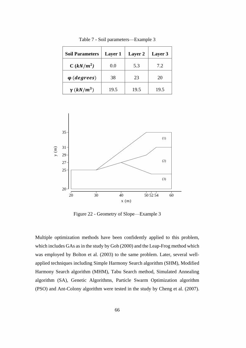
66

Table 7 - Soil parameters—Example 3

Soil Parameters Layer 1 Layer 2 Layer 3

C (𝒌𝑵/𝒎𝟐) 0.0 5.3 7.2

𝛗 (𝒅𝒆𝒈𝒓𝒆𝒆𝒔) 38 23 20

𝛄 (𝒌𝑵/𝒎𝟑) 19.5 19.5 19.5

Figure 22 - Geometry of Slope—Example 3

Multiple optimization methods have been confidently applied to this problem,

which includes GAs as in the study by Goh (2000) and the Leap-Frog method which

was employed by Bolton et al. (2003) to the same problem. Later, several well-

applied techniques including Simple Harmony Search algorithm (SHM), Modified

Harmony Search algorithm (MHM), Tabu Search method, Simulated Annealing

algorithm (SA), Genetic Algorithms, Particle Swarm Optimization algorithm

(PSO) and Ant-Colony algorithm were tested in the study by Cheng et al. (2007).

20 30 40 50 52 54 60

20

25

27

29

31

35

x (m)

y(m

)

(1)

(2)

(3)

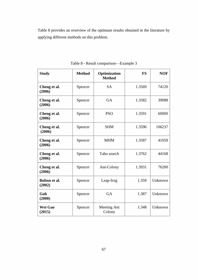
67

Table 8 provides an overview of the optimum results obtained in the literature by

applying different methods on this problem.

Table 8 - Result comparison—Example 3


Method

FS NOF

Cheng et al.

(2006)

Spencer SA 1.3569 74120

Cheng et al.

(2006)

Spencer GA 1.3582 39088

Cheng et al.

(2006)

Spencer PSO 1.3591 60000

Cheng et al.

(2006)

Spencer SHM 1.3596 106237

Cheng et al.

(2006)

Spencer MHM 1.3587 41059

Cheng et al.

(2006)

Spencer Tabu search 1.3762 44168

Cheng et al.

(2006)

Spencer Ant-Colony 1.3931 76200

Bolton et al.

(2002)

Spencer Leap-frog 1.359 Unknown

Goh

(2000)

Spencer GA 1.387 Unknown

Wei Gao

(2015)

Spencer Meeting Ant

Colony

1.348 Unknown

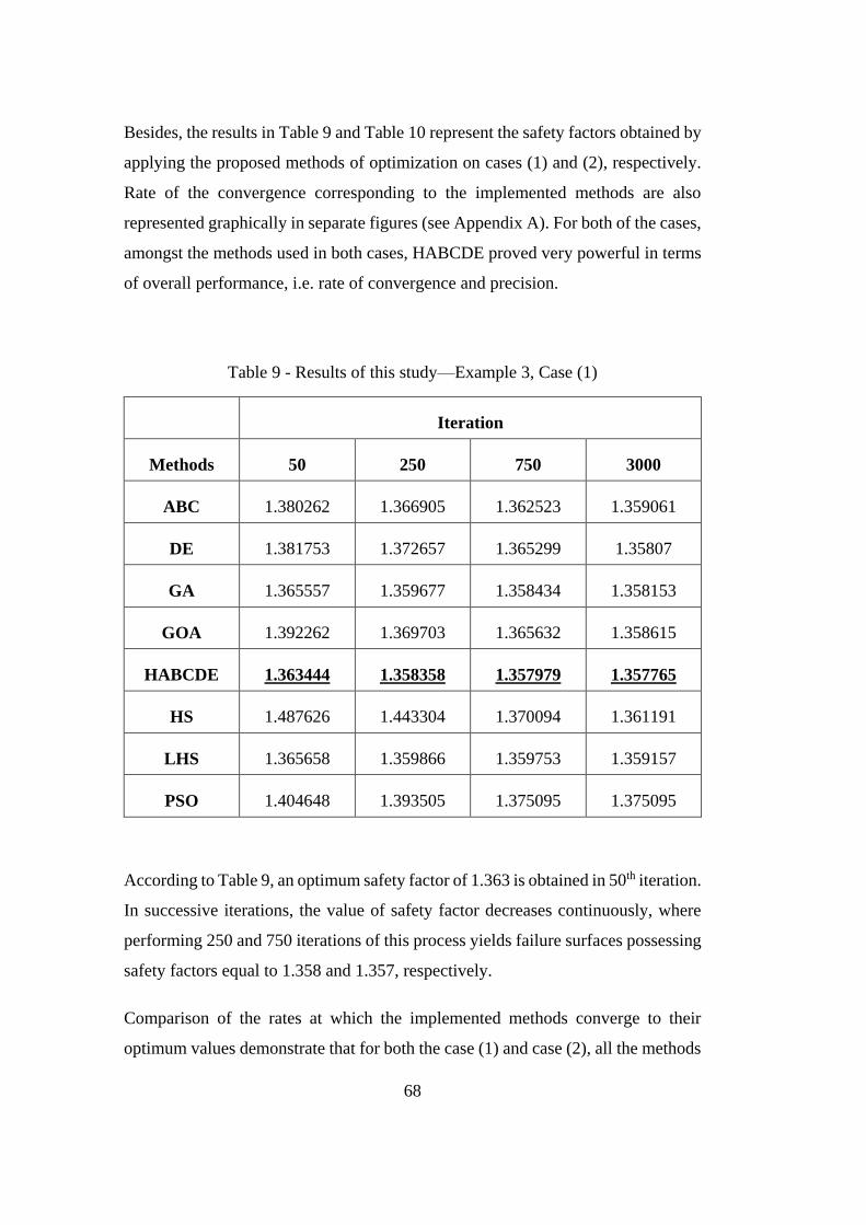
68

Besides, the results in Table 9 and Table 10 represent the safety factors obtained by

applying the proposed methods of optimization on cases (1) and (2), respectively.

Rate of the convergence corresponding to the implemented methods are also

represented graphically in separate figures (see Appendix A). For both of the cases,

amongst the methods used in both cases, HABCDE proved very powerful in terms

of overall performance, i.e. rate of convergence and precision.

Table 9 - Results of this study—Example 3, Case (1)

Iteration

Methods 50 250 750 3000

ABC 1.380262 1.366905 1.362523 1.359061

DE 1.381753 1.372657 1.365299 1.35807

GA 1.365557 1.359677 1.358434 1.358153

GOA 1.392262 1.369703 1.365632 1.358615

HABCDE 1.363444 1.358358 1.357979 1.357765

HS 1.487626 1.443304 1.370094 1.361191

LHS 1.365658 1.359866 1.359753 1.359157

PSO 1.404648 1.393505 1.375095 1.375095

According to Table 9, an optimum safety factor of 1.363 is obtained in 50th iteration.

In successive iterations, the value of safety factor decreases continuously, where

performing 250 and 750 iterations of this process yields failure surfaces possessing

safety factors equal to 1.358 and 1.357, respectively.


optimum values demonstrate that for both the case (1) and case (2), all the methods

69

except the PSO and the HS reach nearly similar values at the end of the analyses

(Figure 23a and Figure 25a). The PSO method for both of the cases fails to obtain

an appropriate value. Similarly, HS method represent a relatively weaker

performance resulting in higher factor of safety values, particularly in the case (2)

where relatively high computational efforts is required to reach a reasonable result

for the case of study.

For the remaining methods, however, no significant difference is observed in the

obtained FS values and therefore, performance of the methods can be evaluated in

terms of their rate of convergence. For better illustration, consider the convergence

rate of the ABC and the DE methods in Figure 25a. Lower FS values obtained over

the same number of iterations proves the superiority of the ABC method over the

DE algorithm.



the competition in terms of both convergence rate and precision for both of the

cases, as illustrated in Figure 23b and Figure 25b. Similarly, for both of the cases,

GOA ranks second according to the factor of safety value, and the LHS method

demonstrates the worst performance. In terms of convergence rate, however, LHS

performs better in the case (1) while for the case (2) GOA proves successful.



Appendix A).

70

(a)

(b)

Figure 23 - Comparison of the convergence rates -- Example 3, Case (1)

(a) all the methods (b) proposed methods

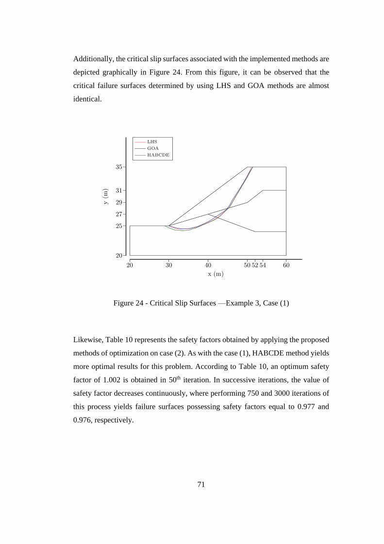
71

Additionally, the critical slip surfaces associated with the implemented methods are

depicted graphically in Figure 24. From this figure, it can be observed that the

critical failure surfaces determined by using LHS and GOA methods are almost

identical.

Figure 24 - Critical Slip Surfaces —Example 3, Case (1)

Likewise, Table 10 represents the safety factors obtained by applying the proposed

methods of optimization on case (2). As with the case (1), HABCDE method yields

more optimal results for this problem. According to Table 10, an optimum safety

factor of 1.002 is obtained in 50th iteration. In successive iterations, the value of

safety factor decreases continuously, where performing 750 and 3000 iterations of

this process yields failure surfaces possessing safety factors equal to 0.977 and

0.976, respectively.

72

Furthermore, visual comparison of the critical failure surfaces from applied

methods is also represented in Figure 26. As can be inferred from this figure the

failure surface passes through the weakest soil layer in the slope profile.

Table 10 - Results of this study—Example 3, Case (2)

Iteration

Methods 50 250 750 3000

ABC 0.99717 0.980165 0.979288 0.979288

DE 1.020548 0.991459 0.98603 0.979214

GA 1.011537 0.983481 0.978353 0.977911

GOA 0.995375 0.978401 0.977525 0.977525

HABCDE 1.002134 0.978964 0.977046 0.976773

HS 1.05532 1.047549 1.010335 0.984624

LHS 1.043134 1.02188 1.02188 0.981427

PSO 1.023048 1.00648 1.003268 0.992467

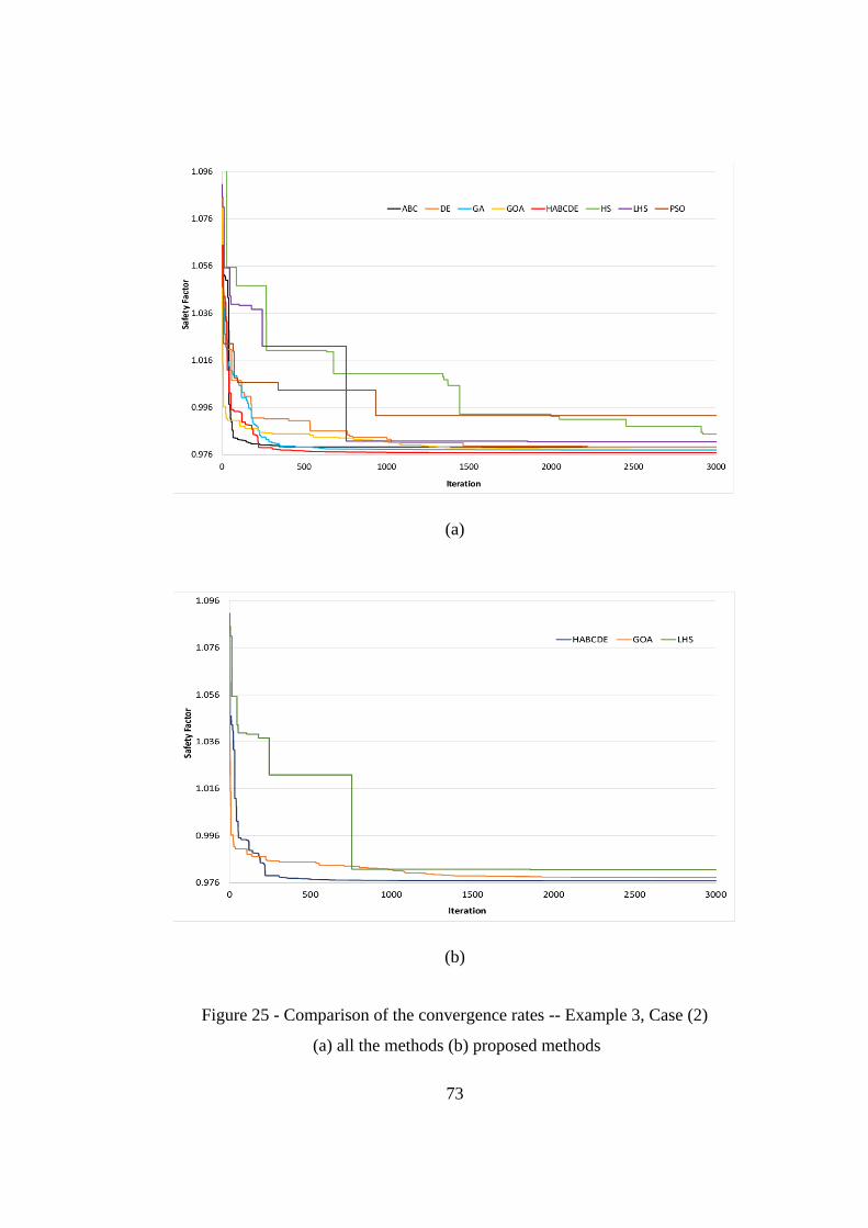
73



(a)

(b)

74

Figure 26 - Critical Slip Surfaces —Example 3, Case (2)

4.4 Case Study 4

Details of the cross-section of a multilayered earth slope is given in the Figure 27.

Stability of this slope against sliding was primarily investigated by Zolfaghari et al.

(2008) using Morgenstern-Price method integrated with GA optimization

technique, given the soil strength parameters outlined in Table 11. In this regard,

four different loading conditions involving water table and earthquake forces were

considered:

Case (1): No water pressure, No earthquake

Case (2): Water pressure, No earthquake

Case (3): No water pressure, Earthquake

Case (4): Water pressure, Earthquake

In addition, a value of 0.1 is considered for the horizontal seismic coefficient of

the earthquake loading acting on the soil mass.

In an effort to enhance the accuracy of stability assessment various optimization

methods have been acceptably applied to this problem; in a study which set out to

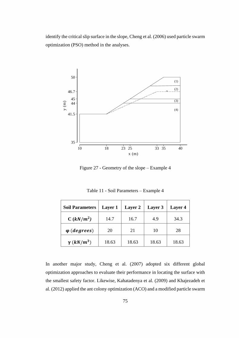
75

identify the critical slip surface in the slope, Cheng et al. (2006) used particle swarm

optimization (PSO) method in the analyses.

Figure 27 - Geometry of the slope – Example 4

Table 11 - Soil Parameters – Example 4

Soil Parameters Layer 1 Layer 2 Layer 3 Layer 4

C (𝒌𝑵/𝒎𝟐) 14.7 16.7 4.9 34.3

𝛗 (𝒅𝒆𝒈𝒓𝒆𝒆𝒔) 20 21 10 28

𝛄 (𝒌𝑵/𝒎𝟑) 18.63 18.63 18.63 18.63

In another major study, Cheng et al. (2007) adopted six different global

optimization approaches to evaluate their performance in locating the surface with

the smallest safety factor. Likewise, Kahatadenya et al. (2009) and Khajezadeh et

al. (2012) applied the ant colony optimization (ACO) and a modified particle swarm

10 18 23 25 33 35 40

35

41.5

4445

46.7

50

x (m)

y(m

)

(1)

(2)

(3)

(4)

76

optimization method (MPSO) to this case problem, respectively. Table 12 provides

an overview of the optimum results obtained in the literature by applying different

methods to this problem.

Table 12 - Result Comparison – Example 4


Method

Case

(1)

Case

(2)

Case

(3)

Case

(4)

Zolfaghari et

al.

(2005)

Spencer GA

1.48 1.36 1.37 0.98 FS

--- --- --- --- NOF

Cheng et al.

(2006) Spencer

SA

1.3961 1.2837 1.1333 1.0081 FS

135560 106742 108542 111386 NOF

GA

1.3733 1.2324 1.0675 0.9631 FS

63562 77178 98332 84272 NOF

PSO

1.3372 1.2100 1.0474 0.9451 FS

62800 83400 69600 68600 NOF

SHM

1.3729 1.2326 1.0733 0.9570 FS

172464 126445 99831 212160 NOF

MHM

1.3501 1.2247 1.0578 0.9411 FS

32510 40697 40476 33236 NOF

Tabu search

1.4802 1.3426 1.1858 1.0848 FS

58588 59790 63796 65398 NOF

Ant-colony

1.5749 1.4488 1.3028 1.1372 FS

100200 102600 109800 112200 NOF

Cheng et al.

(2007) Spencer

Modified

PSO

1.3490 1.2203 1.0592 0.9441 FS

14874 20722 14227 16835 NOF

PSO

1.3323 1.1985 1.0465 0.9225 FS

143919 114865 122744 160060 NOF

Kahatadeniya

et al.

(2009)

MP ACO

1.501 1.377 1.091 0.846 FS

--- --- --- --- NOF

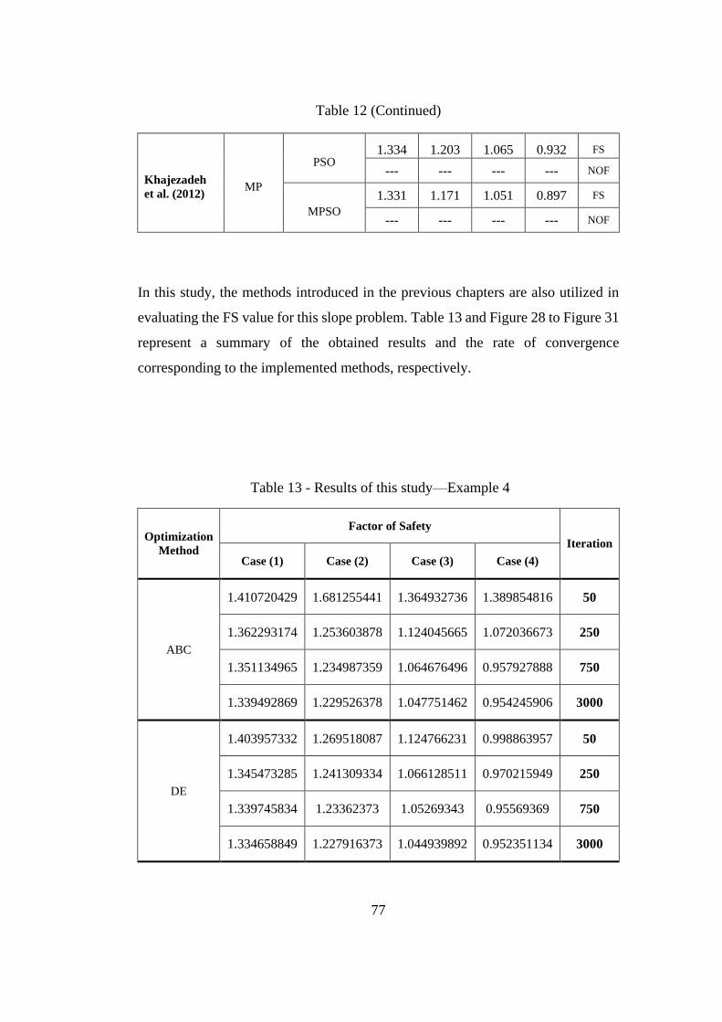
77

Table 12 (Continued)

Khajezadeh

et al. (2012) MP

PSO 1.334 1.203 1.065 0.932 FS

--- --- --- --- NOF

MPSO

1.331 1.171 1.051 0.897 FS

--- --- --- --- NOF

In this study, the methods introduced in the previous chapters are also utilized in

evaluating the FS value for this slope problem. Table 13 and Figure 28 to Figure 31

represent a summary of the obtained results and the rate of convergence

corresponding to the implemented methods, respectively.


Optimization

Method

Factor of Safety

Iteration

Case (1) Case (2) Case (3) Case (4)

ABC

1.410720429 1.681255441 1.364932736 1.389854816 50

1.362293174 1.253603878 1.124045665 1.072036673 250

1.351134965 1.234987359 1.064676496 0.957927888 750

1.339492869 1.229526378 1.047751462 0.954245906 3000

DE

1.403957332 1.269518087 1.124766231 0.998863957 50

1.345473285 1.241309334 1.066128511 0.970215949 250

1.339745834 1.23362373 1.05269343 0.95569369 750

1.334658849 1.227916373 1.044939892 0.952351134 3000

78


GA

1.39091611 1.295484271 1.111094569 1.131368189 50

1.344271501 1.234649087 1.06342718 0.962517243 250

1.338035169 1.231938028 1.049864132 0.954462111 750

1.336644983 1.22971306 1.047404092 0.953760567 3000

GOA

1.375194098 1.269721422 1.07882198 0.98383909 50

1.365378812 1.245432284 1.068523814 0.97747544 250

1.344094069 1.231486596 1.058259522 0.955586733 750

1.3358016 1.227739857 1.047504959 0.953976631 3000

HABCDE

1.342845108 1.345520116 1.055651254 0.969561665 50

1.334481215 1.229676026 1.044547922 0.953873421 250

1.333239328 1.227534324 1.043263764 0.95236442 750

1.332841264 1.22604568 1.043026851 0.950764072 3000

HS

2.446834253 1.692717901 2.130021617 2.165308293 50

1.656123408 1.572059319 1.153395619 1.757718165 250

1.361398095 1.270347238 1.151045628 1.027528563 750

1.339921034 1.234730702 1.056873855 0.967521291 3000

LHS

1.357693435 1.239245752 1.248068043 1.076767521 50

1.351693315 1.233903188 1.065324551 0.965141849 250

1.351170637 1.232030396 1.049893843 0.951786266 750

1.336827587 1.230801909 1.042758288 0.950457457 3000

79


PSO

1.365115673 1.27629403 1.101792138 1.007369006 50

1.365115673 1.27629403 1.082553274 0.976929267 250

1.365115673 1.274486391 1.076631359 0.973040128 750

1.36168701 1.254869993 1.065205964 0.969434701 3000

Comparison of the results obtained in this optimization problem indicates that

HABCDE and LHS outdo their conventional counterparts in terms of accuracy and

convergence rate. In this regard, HABCDE method yields the best results for the

cases (1) and (2). In the third and fourth case, however, the optimum solution is

obtained by LHS method, although HABCDE represents more satisfactory

performance over the earlier iterations.

For better illustration, let us consider the values obtained by the HABCDE method

in the stability analysis of the case (1). According to the Table 13, an optimum

safety factor of 1.3428 is obtained in 50th iteration. Continuing the analyses up to a

higher number of iterations, say 250 and 3000, yields failure surfaces possessing

safety factors equal to 1.3344 and 1.3328, respectively.

In this case of study as well, comparison of the rates at which the implemented

methods converge to their optimum values demonstrate that for both the case (1)

and case (2), the PSO method yields the worst solution for the problem. Similarly,

ABC and HS methods fail to obtain an appropriate factor of safety value,

particularly in the case (1) where relatively high computational efforts are required

to reach a reasonable result for the case of study. Nevertheless, ABC shows a better

performance in the case (2) resulting in a value close to the optimum solution.



80

terms of their rate of convergence. For better illustration, let us consider the

convergence rate of the ABC and the GA methods in the case (2). As represented

in Figure 29a, for both ABC and GA the ultimate factor of safety values are of

similar quantity, while obtaining lower values at the earlier iterations of the GA

method proves its superiority over the ABC algorithm.



the competition in terms of both convergence rate and precision for both case (1)

and (2), as illustrated in Figure 28b and Figure 29b. Additionally, GOA ranks

second according to the overall performance of the methods, i.e. accuracy of the

factor of safety value and the rate of convergence, although LHS performs more

favorably during the initial assessments.

81

(a)

(b)

Figure 28 Comparison of the convergence rates -- Example 4, Case (1)


1.33

1.35

1.37

1.39

1.41

0 500 1000 1500 2000 2500 3000

Safe

ty F

acto

r

Iteration

ABC DE GA GOA HS HABCDE LHS PSO

1.33

1.35

1.37

1.39

1.41

0 500 1000 1500 2000 2500 3000

Safe

ty F

acto

r

Iteration

HABCDE GOA LHS

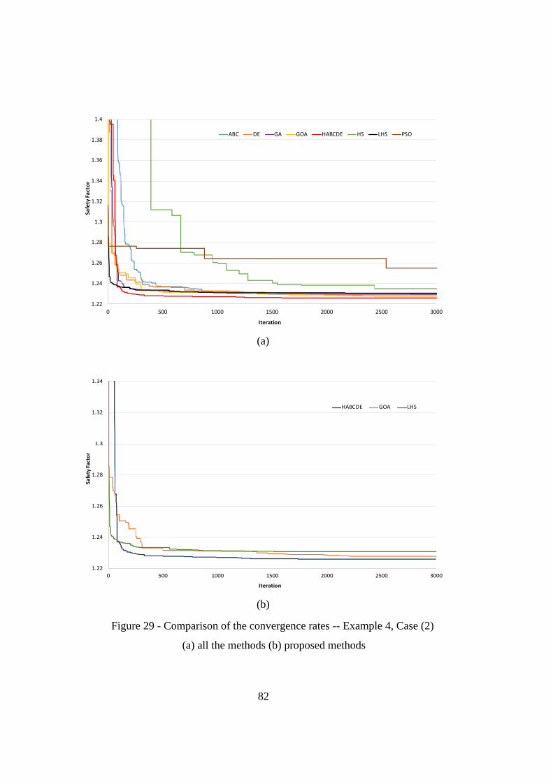
82

(a)

(b)



1.22

1.24

1.26

1.28

1.3

1.32

1.34

1.36

1.38

1.4

0 500 1000 1500 2000 2500 3000

Saf

ety

Fa

cto

r

Iteration

ABC DE GA GOA HABCDE HS LHS PSO

1.22

1.24

1.26

1.28

1.3

1.32

1.34

0 500 1000 1500 2000 2500 3000

Safe

ty F

acto

r

Iteration

HABCDE GOA LHS

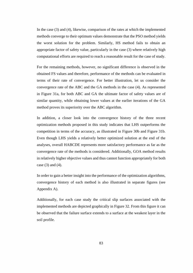
83

In the case (3) and (4), likewise, comparison of the rates at which the implemented

methods converge to their optimum values demonstrate that the PSO method yields

the worst solution for the problem. Similarly, HS method fails to obtain an

appropriate factor of safety value, particularly in the case (3) where relatively high

computational efforts are required to reach a reasonable result for the case of study.



terms of their rate of convergence. For better illustration, let us consider the

convergence rate of the ABC and the GA methods in the case (4). As represented

in Figure 31a, for both ABC and GA the ultimate factor of safety values are of

similar quantity, while obtaining lower values at the earlier iterations of the GA

method proves its superiority over the ABC algorithm.


optimization methods proposed in this study indicates that LHS outperforms the

competition in terms of the accuracy, as illustrated in Figure 30b and Figure 31b.

Even though LHS yields a relatively better optimized solution at the end of the

analyses, overall HABCDE represents more satisfactory performance as far as the

convergence rate of the methods is considered. Additionally, GOA method results

in relatively higher objective values and thus cannot function appropriately for both

case (3) and (4).



Appendix A).

Additionally, for each case study the critical slip surfaces associated with the

implemented methods are depicted graphically in Figure 32. From this figure it can

be observed that the failure surface extends to a surface at the weakest layer in the

soil profile.

84

(a)

(b)



1.04

1.06

1.08

1.1

1.12

1.14

1.16

1.18

1.2

0 500 1000 1500 2000 2500 3000

Safe

ty F

act

or

Iteration

ABC DE GA GOA HABCDE HS LHS PSO

1.04

1.06

1.08

1.1

1.12

1.14

0 500 1000 1500 2000 2500 3000

Safe

ty F

acto

r

Iteration

HABCDE GOA LHS

85

(a)

(b)



0.95

0.97

0.99

1.01

0 500 1000 1500 2000 2500 3000

Safe

ty F

acto

r

Iteration

HABCDE GOA LHS

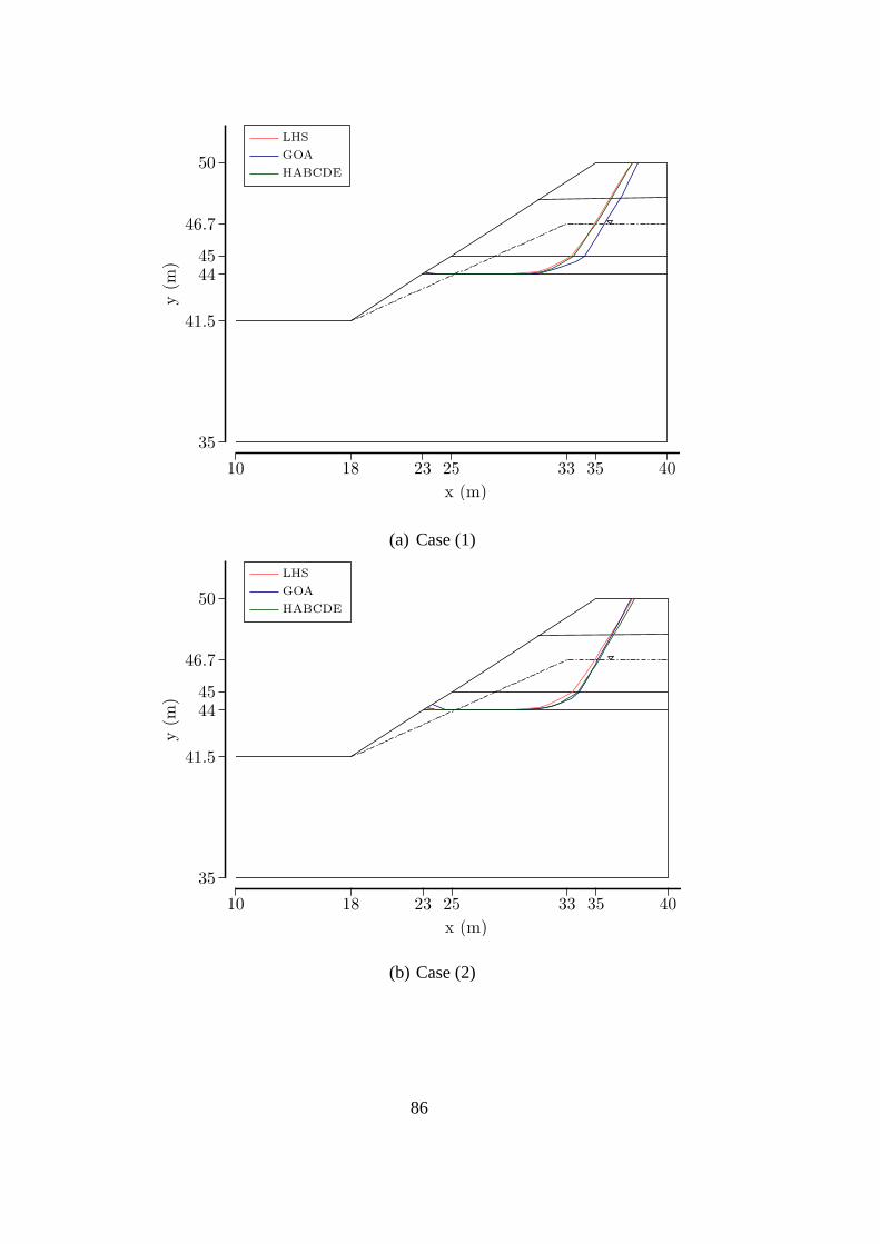
86

(a) Case (1)

(b) Case (2)

87

(c) Case (3)

(d) Case (4)

Figure 32 – Critical Slip Surfaces – Example 4

89

CHAPTER 5

5.SUMMARY AND CONCLUSION

5.1 Summary

Investigating the safety of infrastructures against instabilities is a continuing

concern in civil engineering, which necessitates comprehensive slope stability

analyses to be conducted prior to major construction activities. This helps the

engineers identify the vulnerable zone within the slope profile, providing crucial

insights into the earth condition in the construction site. As a result, realistic

quantification of the safety of the structure against potential failures is of great

importance in the slope stability analysis.

In this study, an effective analysis framework is developed to evaluate the factor of

safety of earth slopes on the basis of limit equilibrium methods. Stability analyses

in this framework are performed in three main steps, which include (1) generating

a number of trial slip surfaces, (2) evaluating safety factors corresponding to the

generated surfaces and lastly, (3) looking for the most critical failure surface

possessing the minimum safety factor. A non-circular surface generation technique

that is capable of forming admissible slip surfaces, i.e. concave upward surfaces, is

efficiently adopted for this purpose. In addition, Among the methods developed for

the slope stability analysis a simplified form of Morgenstern-Price approach that

has found widespread application in practice is implemented in evaluating the

corresponding safety factors along each failure surface. However, the most

challenging step in a complete slope stability analysis is the fast and accurate

localization of the potential failure surface within the slope concurrent with the

determination of the relating FS value, which reflects the minimum factor of safety

of the case study. This objective is too challenging to accomplish considering the

broad diversity of slope problems in geometry, geotechnical parameters of the soil,

90

the depth of the groundwater table, and condition of the external loadings. Robust

optimization techniques, however, have recently performed well in tackling such

difficulties. In this regard, the factor of safety equation is generally considered as

the objective function of the optimization problem and a thorough minimization

process is performed to explore the optimum solution in the search space. In this

study, three recently developed metaheuristic methods that has shown satisfactory

performance on various real-world optimization problems in terms of both

reliability and validity, are implemented.

The applicability of the proposed analysis framework for the slope stability

assessments is subsequently investigated considering several widely-used

numerical examples. Furthermore, in order to gain a better understanding of the

impact of variations in ground conditions on the overall stability of slopes, four case

studies, from simple homogeneous to multi-layered heterogeneous earth slopes

with varied geometries and stratifications, are thoroughly analyzed.

5.2 Findings of the Study

The significance of the quantitative stability analysis of earth slopes as well as the

determination of the surface along which failure is expected has been widely

acknowledged. To date, optimization techniques of different kinds have helped

researchers evaluate how stable is the case of study through completing a fast and

relatively simple procedure. In this study, three recent optimization algorithms,

namely hybrid artificial bee colony with differential evolution, (HABCDE),

grasshopper optimization algorithm (GOA) and improved harmony search

algorithm (LHS) are implemented so as to calculate the lowest FS value pertaining

to the surface of high failure probability. This objective is achieved by minimizing

an objective function (factor of safety) which is defined based on a concise form of

Morgenstern-Price algorithm. Slip surface of the slope is considered to be of non-

circular geometry to provide a better approximation to the actual failure. A set of

three numerical examples with varying geometry and loading conditions are studied

to measure the computational performance of the proposed methods, as well as to

91

benchmark the results against their competitors, as illustrated in the respective

tables. Besides, several illustrative figures for each case study are provided to give

a deeper understanding of the accuracy and convergence rate of the methods along

with a schematic visualization of the expected sliding surfaces, respectively. The

obtained results indicated acceptable and comparable performance for the proposed

method relative to common optimization techniques already used in the analysis of

the same problems. However, when accuracy and convergence rate are used to

evaluate performance, HABCDE outperformed its counterparts, yielding more

optimal results with less computational effort. Consequently, HABCDE proved to

be a suitable scheme in assessing the stability of slopes. Furthermore, it offers

researchers the chance to discover new solutions, hopefully, improved ones, to a

number of challenging optimization problems in their field of study.

5.3 Future Works

The framework proposed in this study proved successful for the stability evaluation

of various slope problems. However, the following key recommendations are

proposed to improve the functionality of the method:

Results indicate that the methods used for generating trial slip surfaces have a direct

influence on the factor of safety evaluations and thus, different results might be

obtained for the same slope problem in this regard. Furthermore, development of

alternative techniques can offer researchers the opportunity to explore new

solutions, hopefully, improved ones.

The efficiency of the framework developed in this study depends heavily on the

rigorousness of the limit equilibrium method and the robustness of the optimization

methods. In future studies, finite element methods can be used in the analyses which

eliminate the need for preliminary assumptions, e.g. consideration of initial trial

slip surfaces and the inter-slice forces in each slice. In addition, certain

modifications can be made to the algorithms of the optimization methods in order

to enhance their performance in acquiring superior results for each benchmark

problem.

92

The reliability of slope stability assessments relies entirely on the validity of the

values assumed for the soil parameters. In this study, key parameters of the soil

medium, namely friction angle, the coefficient of cohesion, unit weight, and pore

water pressure ratio are considered to be constant throughout the soil mass and

therefore, a deterministic analysis is conducted. However, inherent variabilities and

the errors resulting from improper site investigations can also be taken into account

to quantify the probability of slope failures.

Two-dimensional models are adopted in this study for investigating the failure

mechanism of the slopes. However, available evidence demonstrates that all slope

instabilities in nature are virtually in three-dimensional forms. Consequently, in

order to obtain more realistic and accurate results in the analysis, three-dimensional

models can be adopted. This, however, requires huge computational efforts

compared to conventional two-dimensional assessments.

93

REFERENCES

Abramson, Lee, Sharma, & Boyce. (2002). Slope stability and stabilization

methods. John Wiley & Sons.

Arai, & Tagyo. (1985). Determination of noncircular slip surface giving the

minimum factor of safety in slope stability analysis. Soils and Foundations,

25(1), 43–51.

Baker. (1980). Determination of the Critical Slip Surface. Geomechanics,

4(October 1979), 333–359. https://doi.org/10.1002/nag.1610040405

Baker, & Garber. (1978). Theoretical analysis of the stability of slopes.

Geotechnique, (4). https://doi.org/10.1680/geot.1978.28.4.395

Bolton, Heymann, & Groenwold. (2003). Global search for critical failure surface

in slope stability analysis. Engineering Optimization, 35(1), 51–65.

https://doi.org/10.1080/0305215031000064749

Celestino, & Duncan. (1981). Simplified search for non-circular slip surface. In

Proceedings of the 10th international conference on soil mechanics and

foundation engineering, Stockholm, Sweden (pp. 391–394).

Chen, L.-K., Chen, & Ke. (2015). Investigation of the Freeway No. 3 Landslide in

Taiwan. In Engineering Geology for Society and Territory-Volume 2 (pp.

2093–2096). Springer.

Chen, Z., & Shao. (1988). Evaluation of minimum factor of safety in slope stability

analysis. Canadian Geotechnical Journal, 25(November 1988), 735–748.

https://doi.org/doi:10.1139/t88-084

Cheng, Y. M., Li, & Chi. (2007). Performance studies on six heuristic global

optimization methods in the location of critical slip surface. Computers and

Geotechnics, 34(6), 462–484. https://doi.org/10.1016/j.compgeo.2007.01.004

Cheng, Y. M., Li, Chi, & Wei. (2007). Particle swarm optimization algorithm for

the location of the critical non-circular failure surface in two-dimensional

slope stability analysis. Computers and Geotechnics, 34(2), 92–103.

https://doi.org/10.1016/j.compgeo.2006.10.012

94

Cheng, Y. M., Liang, Chi, & Wei. (2008). Determination of the Critical Slip Surface

Using Artificial Fish Swarms Algorithm. Journal of Geotechnical and

Geoenvironmental Engineering, 134(2), 244–251.

https://doi.org/10.1061/(ASCE)1090-0241(2008)134:2(244)

Cheng, Y. M, & Lau. (2008). Slope Stability Analysis and Stabilization: New

Methods and Insight.

Cheng, Y.M., Li, Lansivaara, Chi, & Sun. (2008). An improved harmony search

minimization algorithm using different slip surface generation methods for

slope stability analysis. Engineering Optimization, 40(2), 95–115.

https://doi.org/10.1080/03052150701618153

Cheng, Y, & Lau. (2014). Slope Stability Analysis and Stabilization.

https://doi.org/10.1201/b17015

Cheng, YM, Li, & Lansivaara. (2008). An improved harmony search minimization

algorithm using different slip surface generation methods for slope stability

analysis. Engineering Optimization, 40(2), 95–115.

https://doi.org/10.1080/03052150701618153

Cheng, Yung Ming, Li, Sun, & Au. (2012). A coupled particle swarm and harmony

search optimization algorithm for difficult geotechnical problems. Structural

and Multidisciplinary Optimization, 45(4), 489–501.

https://doi.org/10.1007/s00158-011-0694-z

Das. (2005). Slope stability analysis using genetic algorithm. Electron J Geotech

Eng, 10, 429–439.

Donald, & Giam. (1989). Soil slope stability programs review. Association for

Computer Aided Design (Australia).

Duncan, Wright, & Brandon. (2014). Soil strength and slope stability. John Wiley

& Sons.

Fredlund, & Krahn. (1977). Comparison of slope stability methods of analysis.

Canadian Geotechnical Journal, 14(3), 429–439. https://doi.org/10.1139/t77-

045

Gandomi, Kashani, Mousavi, & Jalalvandi. (2015). Slope stability analyzing using

recent swarm intelligence techniques. International Journal for Numerical

95

and Analytical Methods in Geomechanics, 39(3), 295–309.

Gao. (2015). Slope stability analysis based on immunised evolutionary

programming. Environmental Earth Sciences, 74(4), 3357–3369.

https://doi.org/10.1007/s12665-015-4372-0

Gao. (2016). Premium-penalty ant colony optimization and its application in slope

stability analysis. Applied Soft Computing, 43, 480–488.

https://doi.org/10.1016/j.asoc.2016.03.001

Geem, Kim, & Loganathan. (2001). A new heuristic optimization algorithm:

harmony search. Simulation, 76(2), 60–68.

GOH. (2000). Search for Critical Slip Circle Using Genetic Algorithms. Civil

Engineering and Environmental Systems, 17(3), 181–211.

https://doi.org/10.1080/02630250008970282

Greco. (1996). Efficient Monte Carlo Technique for Locating Critical Slip Surface.

Journal of Geotechnical Engineering, 122(7), 517–525.

https://doi.org/10.1061/(ASCE)0733-9410(1996)122:7(517)

Griffiths, & Lane. (1999). Slope stability analysis by finite elements. Geotechnique,

49(3), 387–403.

Hart. (1995). An introduction to distinct element modeling for rock engineering. In

Analysis and Design Methods (pp. 245–261). Elsevier.

Hu, Jimenez, Li, & Li. (2013). Determination of critical slip surfaces using mutative

scale chaos optimization. Journal of Computing in Civil Engineering, 29(5),

131204001730002. https://doi.org/10.1061/(ASCE)CP.1943-5487.0000373

Jadon, Tiwari, Sharma, & Bansal. (2017). Hybrid Artificial Bee Colony algorithm

with Differential Evolution. Applied Soft Computing, 58, 11–24.


Janbu. (1975). Slope stability computations: In Embankment-dam Engineering.

Textbook. Eds. RC Hirschfeld and SJ Poulos. JOHN WILEY AND SONS

INC., PUB., NY, 1973, 40P. In International Journal of Rock Mechanics and

Mining Sciences & Geomechanics Abstracts (Vol. 12, p. 67). Pergamon.

Jurado-Piña, & Jimenez. (2015). A genetic algorithm for slope stability analyses

with concave slip surfaces using custom operators. Engineering Optimization,

96

47(4), 453–472.

Kahatadeniya, Nanakorn, & Neaupane. (2009). Determination of the critical failure

surface for slope stability analysis using ant colony optimization. Engineering

Geology, 108(1–2), 133–141. https://doi.org/10.1016/j.enggeo.2009.06.010

Kang, Li, & Ma. (2013). An artificial bee colony algorithm for locating the critical

slip surface in slope stability analysis. Engineering Optimization, 45(2), 207–

223.

Karaboga. (2005). An idea based on honey bee swarm for numerical optimization.

Technical report-tr06, Erciyes university, engineering faculty, computer

engineering department.

Kashani, Gandomi, & Mousavi. (2016). Imperialistic Competitive Algorithm: A

metaheuristic algorithm for locating the critical slip surface in 2-Dimensional

soil slopes. Geoscience Frontiers, 7(1), 83–89.

https://doi.org/10.1016/j.gsf.2014.11.005

Khajehzadeh, Raihan Taha, El-Shafie, & Eslami. (2012). Locating the general

failure surface of earth slope using particle swarm optimisation. Civil

Engineering and Environmental Systems, 29(1), 41–57.

https://doi.org/10.1080/10286608.2012.663356

Khajehzadeh, Taha, El-Shafie, & Eslami. (2012). A modified gravitational search

algorithm for slope stability analysis. Engineering Applications of Artificial

Intelligence, 25(8), 1589–1597.

https://doi.org/10.1016/j.engappai.2012.01.011

Li, K. S., & White. (1987). Rapid evaluation of the critical slip surface in slope

stability problems. International Journal for Numerical and Analytical

Methods in Geomechanics, 11(5), 449–473.

Li, Y.-C., Chen, Zhan, Ling, & Cleall. (2010). An efficient approach for locating

the critical slip surface in slope stability analyses using a real-coded genetic

algorithm. Canadian Geotechnical Journal, 47(7), 806–820.

Malkawi, Hassan, & Sarma. (2001). Global Search Method for Locating General

Slip Surface using Monte Carlo Techniques. Journal of Geotechnical and

Geoenvironmental Engineering, 127(8), 688–698. Retrieved from

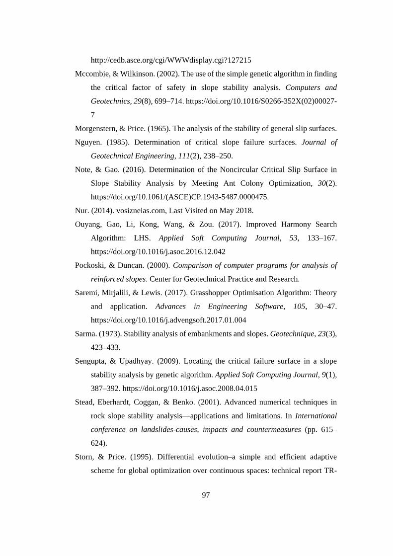
97

http://cedb.asce.org/cgi/WWWdisplay.cgi?127215

Mccombie, & Wilkinson. (2002). The use of the simple genetic algorithm in finding

the critical factor of safety in slope stability analysis. Computers and

Geotechnics, 29(8), 699–714. https://doi.org/10.1016/S0266-352X(02)00027-

7

Morgenstern, & Price. (1965). The analysis of the stability of general slip surfaces.

Nguyen. (1985). Determination of critical slope failure surfaces. Journal of

Geotechnical Engineering, 111(2), 238–250.

Note, & Gao. (2016). Determination of the Noncircular Critical Slip Surface in

Slope Stability Analysis by Meeting Ant Colony Optimization, 30(2).

https://doi.org/10.1061/(ASCE)CP.1943-5487.0000475.

Nur. (2014). vosizneias.com, Last Visited on May 2018.

Ouyang, Gao, Li, Kong, Wang, & Zou. (2017). Improved Harmony Search

Algorithm: LHS. Applied Soft Computing Journal, 53, 133–167.


Pockoski, & Duncan. (2000). Comparison of computer programs for analysis of

reinforced slopes. Center for Geotechnical Practice and Research.

Saremi, Mirjalili, & Lewis. (2017). Grasshopper Optimisation Algorithm: Theory

and application. Advances in Engineering Software, 105, 30–47.

https://doi.org/10.1016/j.advengsoft.2017.01.004

Sarma. (1973). Stability analysis of embankments and slopes. Geotechnique, 23(3),

423–433.

Sengupta, & Upadhyay. (2009). Locating the critical failure surface in a slope

stability analysis by genetic algorithm. Applied Soft Computing Journal, 9(1),

387–392. https://doi.org/10.1016/j.asoc.2008.04.015

Stead, Eberhardt, Coggan, & Benko. (2001). Advanced numerical techniques in

rock slope stability analysis—applications and limitations. In International

conference on landslides-causes, impacts and countermeasures (pp. 615–

624).

Storn, & Price. (1995). Differential evolution–a simple and efficient adaptive

scheme for global optimization over continuous spaces: technical report TR-

98

95-012. International Computer Science, Berkeley, California.

Sun, Li, & Liu. (2008). Search for critical slip surface in slope stability analysis by

spline-based GA method. Journal of Geotechnical and Geoenvironmental

Engineering, 134(2), 252–256. https://doi.org/10.1061/(ASCE)1090-

0241(2008)134:2(252)

Wolpert, & Macready. (1997). No free lunch theorems for optimization. IEEE

Transactions on Evolutionary Computation, 1(1), 67–82.

Yamagami. (1988). Search for noncircular slip surfaces by the Morgenstern-Price

method. In Proc. 6th Int. Conf. Numer. Methods in Geomech. (pp. 1335–

1340).

YAMAGAMI, & JIANG. (1997). A search for the critical slip surface in three-

dimensional slope stability analysis. Soils and Foundations, 37(3), 1–16.

Zhu, D. Y., Lee, & Jiang. (2003). Generalised framework of limit equilibrium

methods for slope stability analysis. Geotechnique.

Zhu, D. Y., Lee, Qian, & Chen. (2005). A concise algorithm for computing the

factor of safety using the MorgensternPrice method. Canadian

Geotechnical Journal, 42(1), 272–278. https://doi.org/10.1139/t04-072

Zhu, G., & Kwong. (2010). Gbest-guided artificial bee colony algorithm for

numerical function optimization. Applied Mathematics and Computation,

217(7), 3166–3173.

Zolfaghari, Heath, & McCombie. (2005). Simple genetic algorithm search for

critical non-circular failure surface in slope stability analysis. Computers and

Geotechnics, 32(3), 139–152. https://doi.org/10.1016/j.compgeo.2005.02.001

99

APPENDIX A

A: CONVERGENCE RATE COMPARISON


convergence history of each method is illustrated in separate figures as follows. A

closer look into the convergence history of the three recent optimization methods

proposed in this study indicates that overall HABCDE represents more satisfactory

performance in the analyses in terms of both convergence rate and accuracy.

(a) (b)

(c) (d)

1.32

1.36

1.4

1.44

0 500 1000 1500 2000 2500 3000

Sa

fety

Fa

cto

r

Iteration

ABC

1.32

1.36

1.4

1.44

0 500 1000 1500 2000 2500 3000

Sa

fety

Fa

cto

r

Iteration

PSO

1.32

1.36

1.4

1.44

0 500 1000 1500 2000 2500 3000

Sa

fety

Fa

cto

r

Iteration

DE

1.32

1.36

1.4

1.44

0 500 1000 1500 2000 2500 3000

Sa

fety

Fa

cto

r

Iteration

HS

100

(e) (f)

(g) (h)

Figure 33- Convergence Rate Comparison – Example 1

1.32

1.36

1.4

1.44

0 500 1000 1500 2000 2500 3000

Sa

fety

Fa

cto

r

Iteration

GA

1.32

1.36

1.4

1.44

0 500 1000 1500 2000 2500 3000

Sa

fety

Fa

cto

r

Iteration

LHS

1.32

1.36

1.4

1.44

0 500 1000 1500 2000 2500 3000

Sa

fety

Fa

cto

r

Iteration

HABCDE

1.32

1.36

1.4

1.44

0 500 1000 1500 2000 2500 3000

Sa

fety

Fa

cto

r

Iteration

GOA

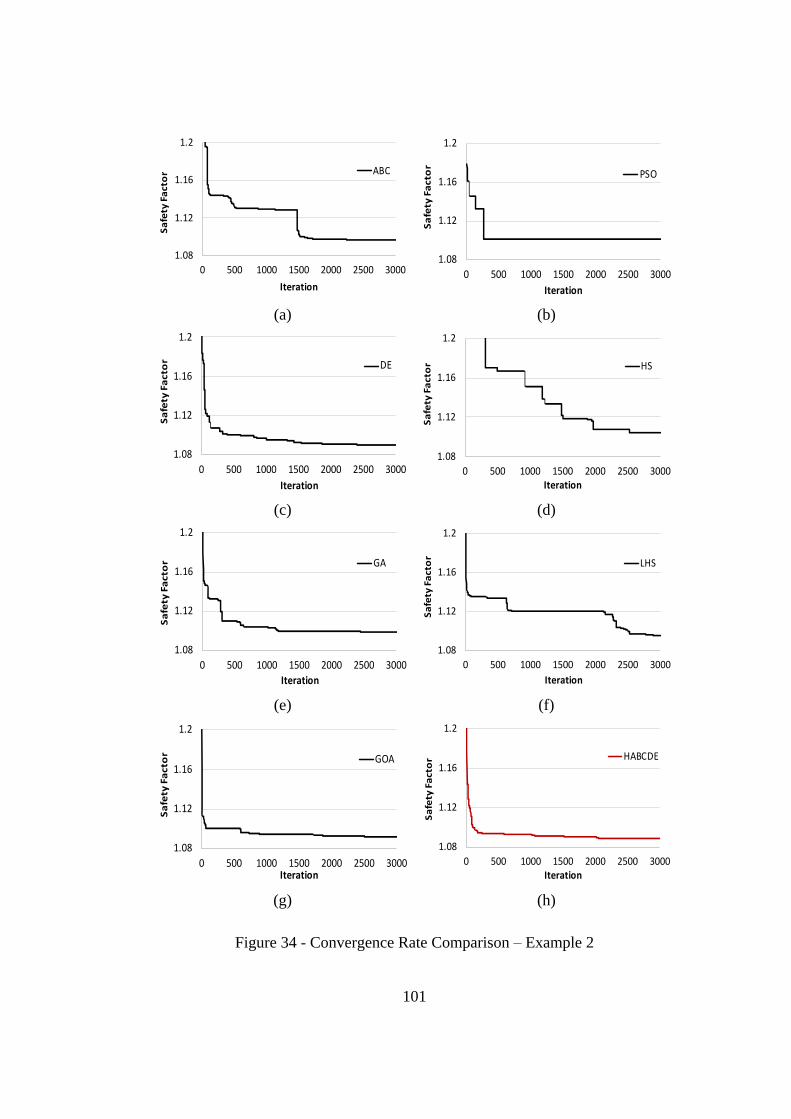
101

(a) (b)

(c) (d)

(e) (f)

(g) (h)

Figure 34 - Convergence Rate Comparison – Example 2

1.08

1.12

1.16

1.2

0 500 1000 1500 2000 2500 3000

Sa

fety

Fa

cto

r

Iteration

ABC

1.08

1.12

1.16

1.2

0 500 1000 1500 2000 2500 3000

Sa

fety

Fa

cto

r

Iteration

PSO

1.08

1.12

1.16

1.2

0 500 1000 1500 2000 2500 3000

Sa

fety

Fa

cto

r

Iteration

DE

1.08

1.12

1.16

1.2

0 500 1000 1500 2000 2500 3000

Sa

fety

Fa

cto

r

Iteration

HS

1.08

1.12

1.16

1.2

0 500 1000 1500 2000 2500 3000

Sa

fety

Fa

cto

r

Iteration

GA

1.08

1.12

1.16

1.2

0 500 1000 1500 2000 2500 3000

Sa

fety

Fa

cto

r

Iteration

LHS

1.08

1.12

1.16

1.2

0 500 1000 1500 2000 2500 3000

Sa

fety

Fa

cto

r

Iteration

GOA

1.08

1.12

1.16

1.2

0 500 1000 1500 2000 2500 3000

Sa

fety

Fa

cto

r

Iteration

HABCDE

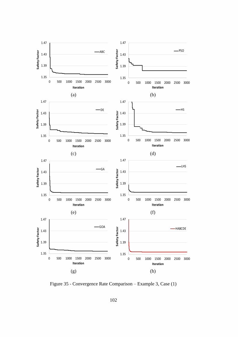
102

(a) (b)

(c) (d)

(e) (f)

(g) (h)

Figure 35 - Convergence Rate Comparison – Example 3, Case (1)

1.35

1.39

1.43

1.47

0 500 1000 1500 2000 2500 3000

Sa

fety

Fa

cto

r

Iteration

ABC

1.35

1.39

1.43

1.47

0 500 1000 1500 2000 2500 3000

Sa

fety

Fa

cto

r

Iteration

PSO

1.35

1.39

1.43

1.47

0 500 1000 1500 2000 2500 3000

Sa

fety

Fa

cto

r

Iteration

DE

1.35

1.39

1.43

1.47

0 500 1000 1500 2000 2500 3000

Sa

fety

Fa

cto

r

Iteration

HS

1.35

1.39

1.43

1.47

0 500 1000 1500 2000 2500 3000

Sa

fety

Fa

cto

r

Iteration

GA

1.35

1.39

1.43

1.47

0 500 1000 1500 2000 2500 3000

Sa

fety

Fa

cto

r

Iteration

LHS

1.35

1.39

1.43

1.47

0 500 1000 1500 2000 2500 3000

Sa

fety

Fa

cto

r

Iteration

GOA

1.35

1.39

1.43

1.47

0 500 1000 1500 2000 2500 3000

Sa

fety

Fa

cto

r

Iteration

HABCDE

103

(a) (b)

(c) (d)

(e) (f)

(g) (h)


0.97

1

1.03

1.06

1.09

0 500 1000 1500 2000 2500 3000

Sa

fety

Fa

cto

r

Iteration

ABC

0.97

1

1.03

1.06

1.09

0 500 1000 1500 2000 2500 3000

Sa

fety

Fa

cto

r

Iteration

PSO

0.97

1

1.03

1.06

1.09

0 500 1000 1500 2000 2500 3000

Sa

fety

Fa

cto

r

Iteration

DE

0.97

1

1.03

1.06

1.09

0 500 1000 1500 2000 2500 3000

Sa

fety

Fa

cto

r

Iteration

HS

0.97

1

1.03

1.06

1.09

0 500 1000 1500 2000 2500 3000

Sa

fety

Fa

cto

r

Iteration

GA

0.97

1

1.03

1.06

1.09

0 500 1000 1500 2000 2500 3000

Sa

fety

Fa

cto

r

Iteration

LHS

0.97

1

1.03

1.06

1.09

0 500 1000 1500 2000 2500 3000

Sa

fety

Fa

cto

r

Iteration

GOA

0.97

1

1.03

1.06

1.09

0 500 1000 1500 2000 2500 3000

Sa

fety

Fa

cto

r

Iteration

HABCDE

104

(a) (b)

(c) (d)

(e) (f)

(g) (h)


1.32

1.38

1.44

1.5

1.56

1.62

0 500 1000 1500 2000 2500 3000

Sa

fety

Fa

cto

r

Iteration

ABC

1.32

1.38

1.44

1.5

1.56

1.62

0 500 1000 1500 2000 2500 3000

Sa

fety

Fa

cto

r

Iteration

PSO

1.32

1.38

1.44

1.5

1.56

1.62

0 500 1000 1500 2000 2500 3000

Sa

fety

Fa

cto

r

Iteration

DE

1.32

1.38

1.44

1.5

1.56

1.62

0 500 1000 1500 2000 2500 3000

Sa

fety

Fa

cto

r

Iteration

HS

1.32

1.38

1.44

1.5

1.56

1.62

0 500 1000 1500 2000 2500 3000

Sa

fety

Fa

cto

r

Iteration

GA

1.32

1.38

1.44

1.5

1.56

1.62

0 500 1000 1500 2000 2500 3000

Sa

fety

Fa

cto

r

Iteration

LHS

1.32

1.38

1.44

1.5

1.56

1.62

0 500 1000 1500 2000 2500 3000

Sa

fety

Fa

cto

r

Iteration

GOA

1.32

1.38

1.44

1.5

1.56

1.62

0 500 1000 1500 2000 2500 3000

Sa

fety

Fa

cto

r

Iteration

HABCDE

105

(a) (b)

(c) (d)

(e) (f)

(g) (h)


1.22

1.26

1.3

1.34

1.38

1.42

0 500 1000 1500 2000 2500 3000

Sa

fety

Fa

cto

r

Iteration

ABC

1.22

1.26

1.3

1.34

1.38

1.42

0 500 1000 1500 2000 2500 3000

Sa

fety

Fa

cto

r

Iteration

PSO

1.22

1.26

1.3

1.34

1.38

1.42

0 500 1000 1500 2000 2500 3000

Sa

fety

Fa

cto

r

Iteration

DE

1.22

1.26

1.3

1.34

1.38

1.42

0 500 1000 1500 2000 2500 3000

Sa

fety

Fa

cto

r

Iteration

HS

1.22

1.26

1.3

1.34

1.38

1.42

0 500 1000 1500 2000 2500 3000

Sa

fety

Fa

cto

r

Iteration

GA

1.22

1.26

1.3

1.34

1.38

1.42

0 500 1000 1500 2000 2500 3000

Sa

fety

Fa

cto

r

Iteration

LHS

1.22

1.26

1.3

1.34

1.38

1.42

0 500 1000 1500 2000 2500 3000

Sa

fety

Fa

cto

r

Iteration

GOA

1.22

1.26

1.3

1.34

1.38

1.42

0 500 1000 1500 2000 2500 3000

Sa

fety

Fa

cto

r

Iteration

HABCDE

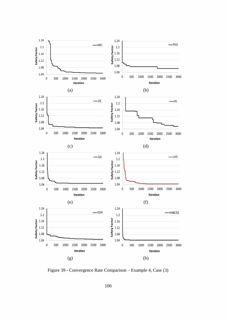
106

(a) (b)

(c) (d)

(e) (f)

(g) (h)


1.04

1.08

1.12

1.16

1.2

1.24

0 500 1000 1500 2000 2500 3000

Sa

fety

Fa

cto

r

Iteration

ABC

1.04

1.08

1.12

1.16

1.2

1.24

0 500 1000 1500 2000 2500 3000

Sa

fety

Fa

cto

r

Iteration

PSO

1.04

1.08

1.12

1.16

1.2

1.24

0 500 1000 1500 2000 2500 3000

Sa

fety

Fa

cto

r

Iteration

DE

1.04

1.08

1.12

1.16

1.2

1.24

0 500 1000 1500 2000 2500 3000

Sa

fety

Fa

cto

r

Iteration

HS

1.04

1.08

1.12

1.16

1.2

1.24

0 500 1000 1500 2000 2500 3000

Sa

fety

Fa

cto

r

Iteration

GA

1.04

1.08

1.12

1.16

1.2

1.24

0 500 1000 1500 2000 2500 3000

Sa

fety

Fa

cto

r

Iteration

LHS

1.04

1.08

1.12

1.16

1.2

1.24

0 500 1000 1500 2000 2500 3000

Sa

fety

Fa

cto

r

Iteration

GOA

1.04

1.08

1.12

1.16

1.2

1.24

0 500 1000 1500 2000 2500 3000

Sa

fety

Fa

cto

r

Iteration

HABCDE

107

(a) (b)

(c) (d)

(e) (f)

(g) (h)


0.9

0.95

1

1.05

1.1

1.15

0 500 1000 1500 2000 2500 3000

Sa

fety

Fa

cto

r

Iteration

ABC

0.9

0.95

1

1.05

1.1

1.15

0 500 1000 1500 2000 2500 3000

Sa

fety

Fa

cto

r

Iteration

PSO

0.9

0.95

1

1.05

1.1

1.15

0 500 1000 1500 2000 2500 3000

Sa

fety

Fa

cto

r

Iteration

DE

0.9

0.95

1

1.05

1.1

1.15

0 500 1000 1500 2000 2500 3000

Sa

fety

Fa

cto

r

Iteration

HS

0.9

0.95

1

1.05

1.1

1.15

0 500 1000 1500 2000 2500 3000

Sa

fety

Fa

cto

r

Iteration

GA

0.9

0.95

1

1.05

1.1

1.15

0 500 1000 1500 2000 2500 3000

Sa

fety

Fa

cto

r

Iteration

LHS

0.9

0.95

1

1.05

1.1

1.15

0 500 1000 1500 2000 2500 3000

Sa

fety

Fa

cto

r

Iteration

GOA

0.9

0.95

1

1.05

1.1

1.15

0 500 1000 1500 2000 2500 3000

Sa

fety

Fa

cto

r

Iteration

HABCDE

application of recent optimization algorithms on …

Documents