application of remote sensing techniques and environmental ... · application of remote sensing...

J. Bio. & Env. Sci. 2015

333 | Nafooti et al.

RESEARCH PAPER OPEN ACCESS

Application of remote sensing techniques and environmental

factors in separating and determining characteristics of

vegetation (Case Study: Siahkooh Basin-Yazd)

M. hassanzadeh Nafooti1, N. Baghestani Meybodi2, Z. Ebrahimi Khusfi3, M. chabok4,

M. Ebrahimi Khusfi5

1Dept. of watershed management, Maybod Branch, Islamic Azad University, Maybod, Iran

2Research Institute of Agriculture and Natural Resources, Yazd, Iran

3College of Natural Resources and Earth Sciences, Kashan University, Iran

4Watershed management, Islamic Azad University, Maybod, Iran

5Remote Sensing and Geographic Information System, Dept. of Remote Sensing and GIS,

Geography Faculty, University of Tehran, Tehran, Iran

Article published on January 12, 2015

Key words: Vegetation fraction, Remote Sensing, Index, Environmental factors, Siahkooh, Iran.

Abstract

Considering the capabilities of satellite imagery and Remote Sensing techniques, researchers employ these as a

conventional method for exploring deserts and research carried out in arid regions. This study aims to evaluate

the application of remote sensing techniques and climatic and geological factors in the separating and

determining characteristics of vegetation in arid regions, especially in Siahkooh basin located in the province of

Yazd (Iran). At first, in order to detect the vegetation fraction in the study area, 286 plots were sampled in the

fieldwork. After applying the necessary preprocessing on the ASTER satellite imagery including the geometric

and radiometric corrections, the soil line equation and 13 vegetation indices were calculated. To study the effect

of environmental factors on the vegetation fraction, information layers such as geology formations, elevation,

slope, aspect, temperature and precipitation were produced and standardized. In order to combine the mentioned

layers and investigate the effect of each factor, the backward elimination method was used for training plots.

Finally, the accuracy of models was assessed based on the correlation coefficient between measured and

estimated values in the test plots. The results of this study showed that MSAVI1 is the most suitable index for

estimating vegetation fraction in the case study. Furthermore, the results indicated that climatic and geological

factors do not have any significant effect on increasing the accuracy of the models in Siahkooh basin.

*Corresponding Author: M.Hasanzadeh Nafooti [email protected]

Journal of Biodiversity and Environmental Sciences (JBES)

ISSN: 2220-6663 (Print), 2222-3045 (Online)

http://www.innspub.net

Vol. 6, No. 1, p. 333-343, 2015

mailto:[email protected]



Introduction

Iran is located in an arid and semi-arid part of the

world with an area of 1.65 million SQKM. Deserts and

arid lands comprise a major part of its area. Among

these, Yazd province can be named as one of the

major arid parts of Iran, a desert, and it is important

to obtain information about its vegetation amount

and distribution. Satellite data provide possibility for

investigating vegetation cover. In order to reduce the

effect of undesired factors on vegetation and increase

information, vegetation indices were used. Sparse

vegetation in most parts of the country has provided

special conditions for reflection. Sparse vegetation in

these areas leads to soil affecting vegetation

reflectance and dominating it (Griffiths.,1985).

Furthermore, reflectance from a surface with

vegetation is a combination of reflectance from leaves

and soil, and therefore differentiating them from one

another makes it difficult to use satellite data

(Hayez.,1997).

During the last decades, using a vegetation index is

common in order to determine physical

characteristics of vegetative cover. These indices are

usually calculated by using a combination of visible

and infrared bands and have showed good

correlation with vegetation growth, vegetation

percentage and biomass amount (Rondeaux et al.,

1996). Casanava et al., (1998) used Landsat imagery

and PVI, NDVI, RVI and WDVI indices to determine

the cover percentage and biomass of rice. They

concluded that WDVI and PVI indices can better

indicate percent vegetation cover . In arid areas, due

to the double effect of soil reflection on NDVI, it

cannot indicate vegetation characteristics and

decreases the accuracy of estimating vegetation

fraction in these regions (Ishiyama et.al.,1997).

Vegetation indices which consider soil reflection can

better show the vegetation characteristics (Kallel et

al., 2007; Darvishzadeh et al., 2008). Ju et al.,

(2008) concluded that the NDVI index is not an

indicator of percent vegetation cover because of

heterogeneous topography; therefore, Artificial

Neural Networks (ANN) was used as a suitable

modelbased on the topography of the study area in

order to determine percent vegetation cover. In a

study about one of the arid areas located in Colorado,

USA, Baugh and Groeneveld (2006) concluded that

NDVI is better than vegetation indices for showing

percent vegetation cover in arid regions. They used

Landsat imagery taken within a 14 year time period

and results showed higher accuracy of the NDVI

index in comparison to other indices (DVI, IPVI,

TSAVI, SAVI). Ghaemi et al., (2009) introduced

SAVI, TVI, NDSI, NDVI, SI, BI1, RI, VI1, VI6, VI5,

MSR, COSRI, MSAVI in studying the vegetative

indices of Nishaboor plain and the first and third

components were obtained by principal component

analysis and light and chlorophyll bands showed to be

the best indices for identifying and differentiation of

vegetation. Behbahani et al., (2010) introduced the

NDVI and MSAVI indices of ASTER as the best

indices for determining the percentage of trees

canopy for arid zones. When determining the percent

vegetation cover in Samirom rangelands using AWiFS

images, Jabbari et al., (2011) showed that rangelands

with 20-30 and 30-40 vegetation classes are located

at high altitudes and low slopes. Cabasinha and

Castro (2009) determined the relationship between

vegetation diversity of 22 parcels of forest and 5

vegetation indices (NDVI, SAVI, EVI, MVI5, MVI7),

structure and area geometry using TM imagery.

Results showed that EVI has a significant correlation

with vegetation diversity but MVI5 has no significant

correlation with vegetation diversity. Yang et al.,

(2013) implemented seasonal variation of percent

vegetation cover based on analyzing spectral model

and remote sensing in mountain regions. Results

showed that there is a strong correlation (0.85) and

low least error squares (0.08) between percent

vegetation measured through field studies and

estimated percent of remote sensing data. They

showed that vegetation diversity reaches its

maximum in May and June in the study area. Koide

and Koike (2012) used indices of SPOT images in

order to determine areas with high underground

water table in warm and humid areas. They’ve also

showed that the new index NDVI is more sensitive to



water tension in vegetation and has a strong linear

correlation with percent vegetation cover in this area

when compared to other indices such as Vis, SAVI

and EVI2. Abdollahi et al., (2007) showed that

synchronous use of several parameters leads to better

conclusion when determining the percentage of

vegetation in arid areas. Arkhy et al., (2011) studied

monitoring change in vegetation using remote

sensing techniques in Ilam dam basin. They showed

that the red band differentiation method has the

highest accuracy among other methods with a total

accuracy of 89 and the Kappa coefficient of 0.82 and

the ratio method of near infrared band has least

accuracy in monitoring vegetation change with a total

accuracy of 64.5 and the Kappa coefficient of 0.24.

The objective of this paper is to evaluate the application

of satellite remote sensing technology and

environmental factors in order to determine the

characteristics of vegetation in arid regions, especially in

Siahkooh Basin located in the province of Yazd (Iran).

Materials and methods

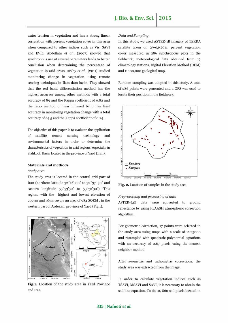
Study area

The study area is located in the central arid part of

Iran (northern latitude 32˚16' 00" to 32˚37' 30" and

eastern longitude 53˚53'30" to 53˚32'30"). This

region, with the highest and lowest elevation of

2077m and 96m, covers an area of 984 SQKM , in the

western part of Ardekan, province of Yazd (Fig.1).

Fig.1. Location of the study area in Yazd Province

and Iran.

Data and Sampling

In this study, we used ASTER-1B imagery of TERRA

satellite taken on 29-03-2011, percent vegetation

cover measured in 286 synchronous plots in the

fieldwork, meteorological data obtained from 19

climatology stations, Digital Elevation Method (DEM)

and 1: 100,000 geological map.

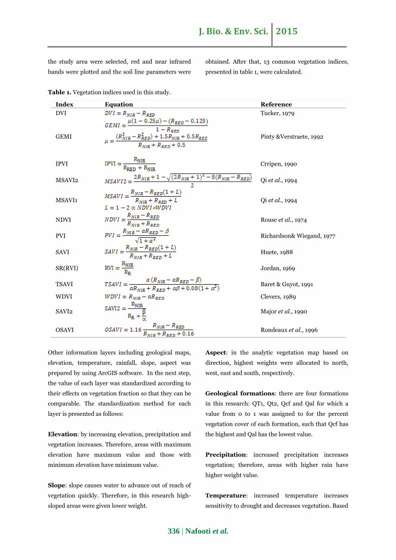
Random sampling was adopted in this study. A total

of 286 points were generated and a GPS was used to

locate their position in the fieldwork.

Fig. 2. Location of samples in the study area.

Preprocessing and processing of data

ASTER-L1B data were converted to ground

reflectance by using FLAASH atmospheric correction

algorithm.

For geometric correction, 17 points were selected in

the study area using maps with a scale of 1: 25000

and resampled with quadratic polynomial equations

with an accuracy of 0.67 pixels using the nearest

neighbor method.

After geometric and radiometric corrections, the

study area was extracted from the image .

In order to calculate vegetation indices such as

TSAVI, MSAVI and SAVI, it is necessary to obtain the

soil line equation. To do so, 860 soil pixels located in



the study area were selected, red and near infrared

bands were plotted and the soil line parameters were

obtained. After that, 13 common vegetation indices,

presented in table 1, were calculated.

Table 1. Vegetation indices used in this study.

Reference Equation Index

Tucker, 1979 DVI

Pinty &Verstraete, 1992

GEMI

Crripen, 1990

IPVI

Qi et al., 1994

MSAVI2

Qi et al., 1994

MSAVI1

Rouse et al., 1974

NDVI

Richardson& Wiegand, 1977

PVI

Huete, 1988

SAVI

Jordan, 1969

SR(RVI)

Baret & Guyot, 1991

TSAVI

Clevers, 1989 WDVI

Major et al., 1990

SAVI2

Rondeaux et al., 1996

OSAVI

Other information layers including geological maps,

elevation, temperature, rainfall, slope, aspect was

prepared by using ArcGIS software. In the next step,

the value of each layer was standardized according to

their effects on vegetation fraction so that they can be

comparable. The standardization method for each

layer is presented as follows:

Elevation: by increasing elevation, precipitation and

vegetation increases. Therefore, areas with maximum

elevation have maximum value and those with

minimum elevation have minimum value.

Slope: slope causes water to advance out of reach of

vegetation quickly. Therefore, in this research high-

sloped areas were given lower weight.

Aspect: in the analytic vegetation map based on

direction, highest weights were allocated to north,

west, east and south, respectively.

Geological formations: there are four formations

in this research: QT1, Qt2, Qcf and Qal for which a

value from 0 to 1 was assigned to for the percent

vegetation cover of each formation, such that Qcf has

the highest and Qal has the lowest value.

Precipitation: increased precipitation increases

vegetation; therefore, areas with higher rain have

higher weight value.

Temperature: increased temperature increases

sensitivity to drought and decreases vegetation. Based



on this, maximum weight was assigned to areas with

minimum temperature and minimum weight was

assigned to areas with maximum temperature.

Vegetation fraction: In order to determine percent

vegetation cover, vegetation indices were used based

on satellite imagery. Areas with dense vegetation

gained higher weight.

Finally, the value of each sample point in all

mentioned layers was then extracted by overlaying

the sample point on these information layers.

Vegetation indices were calculated in MATLAB

software. . The evaluation of obtained results was

carried out by using cross validation methods.

Statistical analysis

One approach to simplifying multiple regression

equations is the stepwise procedures. These include

forward selection, backwards elimination, and

stepwise regression. In this research, we use

backwards elimination method, because this method

has an advantage over forward selection and stepwise

regression because it is possible for a set of variables

to have considerable predictive capability even

though any subset of them does not. Forward

selection and stepwise regression will fail to identify

them. Because the variables don't predict well

individually, they will never get to enter the model to

have their joint behavior noticed. Backwards

elimination starts with everything in the model, so

their joint predictive capability will be seen

(http://www.jerrydallal.com). It is necessary to

mention that in this stage one-third of samples were

used as test samples and two-thirds were used as

training data. Validity of models was measured using

correlation values and estimated values were

evaluated in the location related to test samples.

Results

Equation 2 shows the soil line equation for the study

area.

Equation 2.

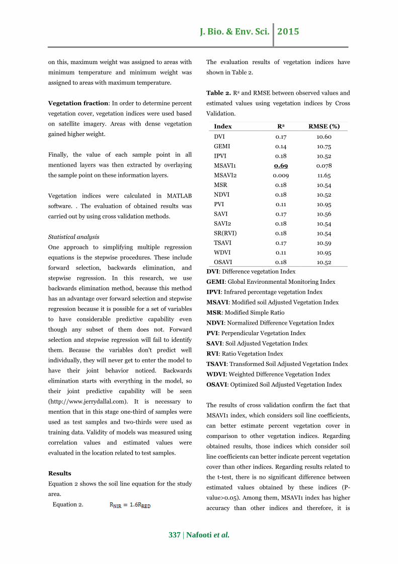
The evaluation results of vegetation indices have

shown in Table 2.

Table 2. R2 and RMSE between observed values and

estimated values using vegetation indices by Cross

Validation.

Index R2 RMSE (%)

DVI 0.17 10.60

GEMI 0.14 10.75

IPVI 0.18 10.52

MSAVI1 0.69 0.078

MSAVI2 0.009 11.65

MSR 0.18 10.54

NDVI 0.18 10.52

PVI 0.11 10.95

SAVI 0.17 10.56

SAVI2 0.18 10.54

SR(RVI) 0.18 10.54

TSAVI 0.17 10.59

WDVI 0.11 10.95

OSAVI 0.18 10.52

DVI: Difference vegetation Index

GEMI: Global Environmental Monitoring Index

IPVI: Infrared percentage vegetation Index

MSAVI: Modified soil Adjusted Vegetation Index

MSR: Modified Simple Ratio

NDVI: Normalized Difference Vegetation Index

PVI: Perpendicular Vegetation Index

SAVI: Soil Adjusted Vegetation Index

RVI: Ratio Vegetation Index

TSAVI: Transformed Soil Adjusted Vegetation Index

WDVI: Weighted Difference Vegetation Index

OSAVI: Optimized Soil Adjusted Vegetation Index

The results of cross validation confirm the fact that

MSAVI1 index, which considers soil line coefficients,

can better estimate percent vegetation cover in

comparison to other vegetation indices. Regarding

obtained results, those indices which consider soil

line coefficients can better indicate percent vegetation

cover than other indices. Regarding results related to

the t-test, there is no significant difference between

estimated values obtained by these indices (P-

value>0.05). Among them, MSAVI1 index has higher

accuracy than other indices and therefore, it is

http://www.jerrydallal.com/LHSP/whole_and_parts.htm



http://www.jerrydallal.com/



selected as the most suitable index. In the next step,

layers related to effective parameters on vegetation

were prepared.

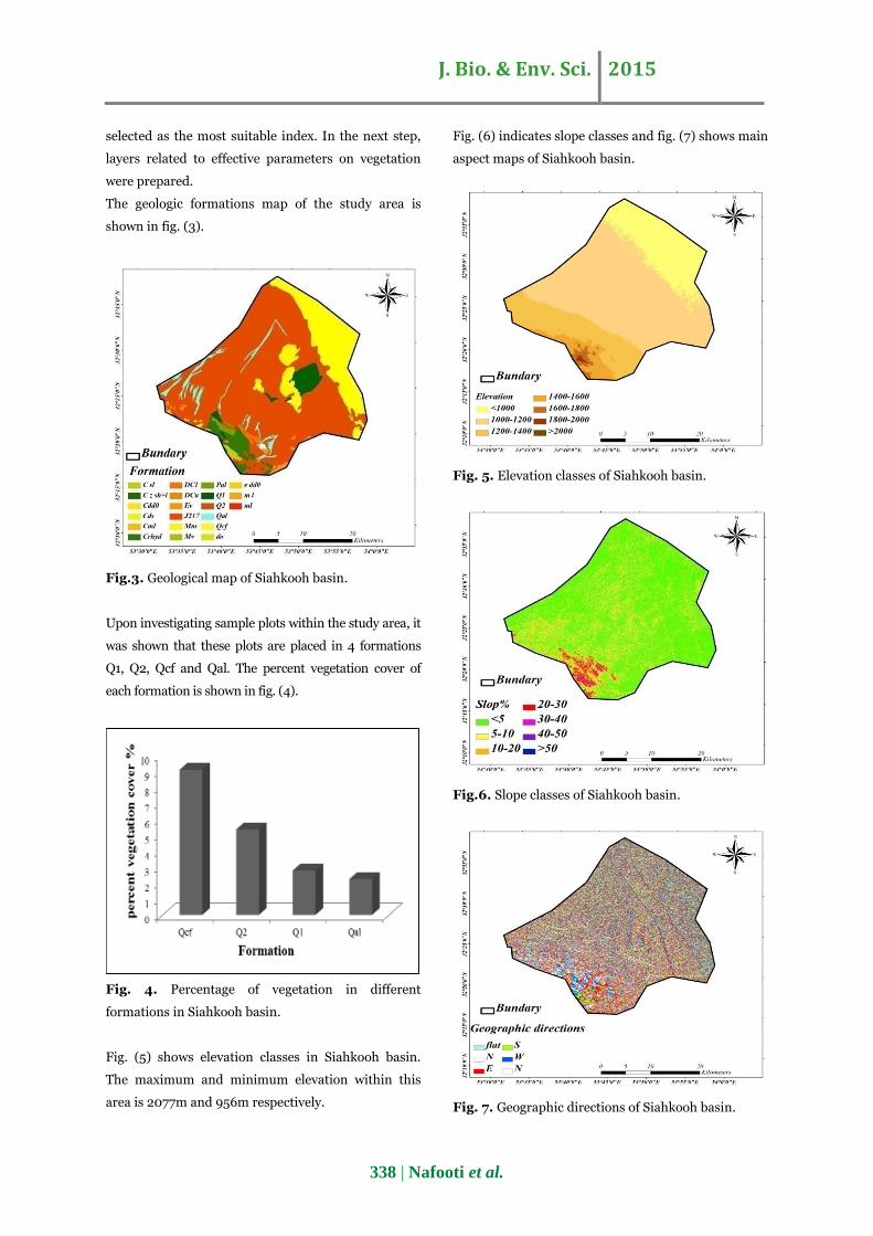
The geologic formations map of the study area is

shown in fig. (3).

Fig.3. Geological map of Siahkooh basin.

Upon investigating sample plots within the study area, it

was shown that these plots are placed in 4 formations

Q1, Q2, Qcf and Qal. The percent vegetation cover of

each formation is shown in fig. (4).

Fig. 4. Percentage of vegetation in different

formations in Siahkooh basin.

Fig. (5) shows elevation classes in Siahkooh basin.

The maximum and minimum elevation within this

area is 2077m and 956m respectively.

Fig. (6) indicates slope classes and fig. (7) shows main

aspect maps of Siahkooh basin.

Fig. 5. Elevation classes of Siahkooh basin.

Fig.6. Slope classes of Siahkooh basin.

Fig. 7. Geographic directions of Siahkooh basin.



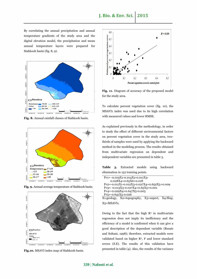
By correlating the annual precipitation and annual

temperature gradients of the study area and the

digital elevation model, the precipitation and mean

annual temperature layers were prepared for

Siahkooh basin (fig. 8, 9).

Fig. 8. Annual rainfall classes of Siahkooh basin.

Fig. 9. Annual average temperature of Siahkooh basin.

Fig.10. MSAVI index map of Siahkooh basin.

Fig. 11. Diagram of accuracy of the proposed model

for the study area.

To calculate percent vegetation cover (fig. 10), the

MSAVI1 index was used due to its high correlation

with measured values and lower RMSE.

As explained previously in the methodology, in order

to study the effect of different environmental factors

on percent vegetation cover in the study area, two-

thirds of samples were used by applying the backward

method in the modeling process. The results obtained

from multivariate regression on dependent and

independent variables are presented in table 3.

Table 3. Extracted models using backward

elimination in 152 training points.

Fv1= -0.019X1-0.014X2-0.011X3- 0.028X4+0.65X6+0.018 Fv2=-0.011X1-0.012X3-0.027X4+0.652X5+0.009 Fv3= -0.013X3-0.027X4+0.65X5+0.001 Fv4=-0.029X4+0.647X5-0.005 Fv5=-0.641X5-0.026

X1:geology, X2=topography, X3=aspect, X4:Slop,

X5=MSAVI1.

Owing to the fact that the high R2 in multivariate

regression does not imply its inefficiency and the

efficiency of a model is confirmed when it can give a

good description of the dependent variable (Rezaie

and Soltani, 1998); therefore, extracted models were

validated based on higher R2, F and lower standard

errors (S.E). The results of this validation have

presented in table (4). Also, the results of the variance



analysis with linear multivariate regression have

presented in table (5).

Table 4. Results of the extracted model evaluation.

Model R R2 R2 adjusted RMSE

1 0.83 0.689 0.678 0.07906

2 0.83 0.688 0.680 0.07882

3 0.829 0.688 0.682 0.07858

4 0.829 0.687 0.683 0.0784

5 0.829 0.686 0.684 0.07827

Table 5. Results of variance analysis using the

multiple linear regression method.

Variation reference

Model

Sum- squares

df Mean-square

F

1 Regression 2.017 5 0.403 64.557 Residuals 0.912 146 0.006 Total 2.93 151





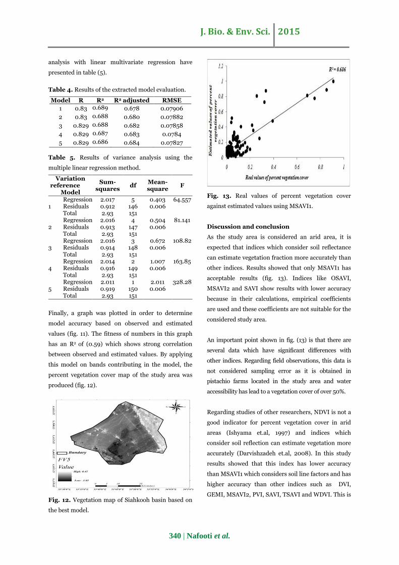
Finally, a graph was plotted in order to determine

model accuracy based on observed and estimated

values (fig. 11). The fitness of numbers in this graph

has an R2 of (0.59) which shows strong correlation

between observed and estimated values. By applying

this model on bands contributing in the model, the

percent vegetation cover map of the study area was

produced (fig. 12).

Fig. 12. Vegetation map of Siahkooh basin based on

the best model.

Fig. 13. Real values of percent vegetation cover

against estimated values using MSAVI1.

Discussion and conclusion

As the study area is considered an arid area, it is

expected that indices which consider soil reflectance

can estimate vegetation fraction more accurately than

other indices. Results showed that only MSAVI1 has

acceptable results (fig. 13). Indices like OSAVI,

MSAVI2 and SAVI show results with lower accuracy

because in their calculations, empirical coefficients

are used and these coefficients are not suitable for the

considered study area.

An important point shown in fig. (13) is that there are

several data which have significant differences with

other indices. Regarding field observations, this data is

not considered sampling error as it is obtained in

pistachio farms located in the study area and water

accessibility has lead to a vegetation cover of over 50%.

Regarding studies of other researchers, NDVI is not a

good indicator for percent vegetation cover in arid

areas (Ishyama et.al, 1997) and indices which

consider soil reflection can estimate vegetation more

accurately (Darvishzadeh et.al, 2008). In this study

results showed that this index has lower accuracy

than MSAVI1 which considers soil line factors and has

higher accuracy than other indices such as DVI,

GEMI, MSAVI2, PVI, SAVI, TSAVI and WDVI. This is



due to allocating empirical factors to indices such as

SAVI and MSAVI2 which reduces accuracy.

GEMI is an index which is presented to reduce

atmospheric effects. This index showed to have low

accuracy in this research. This is because of excessive

soil reflectance in the study area (Liang, 2003). Also,

in calculating this index, various constants are used

which may not be suitable for the study area and

create this error. Results in table (5) showed that

among extracted models, model number 5 is the most

suitable model for estimating percent vegetation

cover in Siahkooh, due to high R2, F and low standard

error. On the other hand, results of fitness for

determining the accuracy of the model in the study

area showed strong correlation (R2= 0.684) between

observed and estimated values. Therefore, model 5 is

the most appropriate model for estimating percent

vegetation cover in the study area. In order to justify

this, one must refer to the variables that have

constructed this model. As the model shows, the

MSAVI1 index has the highest effect in determining

vegetation in the study area. In arid and semi-arid

areas, because of sparse and dispersed vegetation, soil

reflection has a considerable effect on recorded

values, and this is one of the most important points

which should be considered when studying vegetation

of arid areas. There have been many attempts for

minimizing the effects of the environment on the

numerical value of spectral reflection caused by

vegetation in arid areas. For example, Qi et.al (2002)

developed an index named MSAVI which has

significantly reduced the effects of soil reflection. In

this research, by calculating soil coefficients, we tried

to reduce soil reflectance effect and as results showed,

the most suitable model for determining percent

vegetation cover in the study area was MSAVI1. As the

equation related to this index shows, additionally red

and mid-infrared bands which are sensitive to

vegetation, also the coefficients related to the soil line

equation are used and this decreases or eliminates

soil reflectance and increases accuracy. As table (3)

shows, although environmental parameters were

entered into other models but they had no effect in

increasing accuracy and at the last model (5) was

selected as the most suitable model for the study area.

The reason for environmental factors having no effect

in increasing modeling accuracy is low variance of

parameters such as temperature, precipitation, slope

and uniform formations in most sampled plots.

Therefore, it seems that the most significant factor in

showing vegetation in Siahkooh is spectral reflection

of vegetation canopy in sample plots which was

shown with high accuracy using ASTER. This shows

the high capability of ASTER imagery in indicating

the most important characteristic of vegetation in the

study area. It also presents an accurate estimation of

vegetation as well as reducing required time and

costs.

References

Abdullahi J, Baghestani N, Savaghebi MH,

Rahimian MH. 2007. Determination of vegetation

in arid regions using remote sensing and GIS (Case

Study: Watershed Nodoushan). Journal of Science

and Technology of Agriculture and Natural Resources

44, 313-301.

Arkhy S, Niazi Y, Adibnejad M. 2011.

Monitoring vegetation cover changes using remote

sensing techniques in Ilam dam basin. Geography and

Development 24, 133-121.

Baret F, Guyot G. 1991. Potentials and limits of

vegetation indices for LAI and APAR assesment.

Remote Sensing Of Environment 35, 161-173.

Baugh WM, Groeneveld P. 2006. Broadband

vegetation index performance evaluated for a low-

cover environment." International Journal of Remote

Sensing 27,4715-4730.

Behbehani N, Fallah Shamsi SR, Frzadmehr

J, Erfanfard SY, Ramezani M. 2010. Using

vegetation index of ASTER-L1B images in a single

estimate of canopy trees in arid rangelands. Case

Study: Tak Ahmad Shahi - South Khorasan. Journal

of Range Management 4, 103-93.



Cabacinha C, Castro S. 2009. Relationships

between floristic and vegetation indices, forest

structure and landscape metrics of fragments in

Brazilia Cerrado. Forest and Ecology and

Management 257, 2157-2165.

Casanova D, Epema GF, Goudriaan J. 1998.

Monitoring rice reflectance at field level for

estimating biomass and LAI. Field Crops Research

55, 83-92

Clevers JGPW. 1989. The application of a weighted

infrared-red vegetation index for estimating leaf area

index by correcting soil moisture. Remote Sensing Of

Environment 29, 25–37.

Crippen RE. 1990. Calculating the vegetation index

faster. Remote Sensing Of Environment 34, 71–73.

Darvishzadehh R, Skidmore A, Atzberger C,

Wieren S. 2008. Estimation of vegetation LAI from

hyper spectral reflectance data: Effects of soil type

and plant architecture. International Journal of

Applied Earth Observation and Geoinformation, 10,

358-372.

Fox GA, Sabbagh GJ, Searcy SW, Yang C. 2004.

An automated soil line identification routine for

remotely sensed images. Soil Science Society

American Journal 68, 1326-1331.

Ghaemi M, Sanaei Nejad SH, Astaraei AR,

Mirhoseini P. 2009. Comparison of different

vegetation index using ETM+ satellite images for

vegetation studies of Nishapur Plain, Khorasan

Razavi. Journal of Iranian Field Crop Research,

Volume 8, Number 1, 137-128.

Griffiths GH. 1985. Mapping rangeland vegetation

in northern Kenya from Landsat data. PhD. Thesis,

University of Aston in Birmingham, 205pp.

Hayez R. 1997. Principals of Remote Sensing,

Remote Sensing Center of Iran, Tehran University

press, 645pp.

Huete H. 1988. A soil-adjusted vegetation index

(SAVI). Remote Sensing Of Environment 25, 295–309.

Ishiyama T, Nakajima Y, Kajiwara K, Tsuchiya

K. 1997. Extraction of vegetation covers in an arid

area based on satellite data. Advances in Space

Research , Calibration and Intercalibration of Satellite

Sensors and Early Results of Radarsat 19, 1375-1378

Jabbari S, khajedin SJ, Soltani S, Jafari R.

2011. Determination of Range Vegetation Using

Remote Sensing and GIS (Case Study: Semirom).

National Conference on Geomatics, 10 p.

Ju C, Cai T, Yang X. 2008. Topography-based

modeling to estimate percent vegetation cover in

semi-arid Mu Us sandy land, China. Computers and

Electronics in Agriculture 64, 133-139.

Jordan CF. 1969. Derivation of leaf area index from

quality of light on the forest floor .Ecology 50, 663-666.

Kallel A, Sylvie L, Catherine O, Laurence H.

2007. Determination of vegetation cover fraction by

inversion of a four-parameter model based on isoline

parameterization. Remote Sensing Of Environment

111, 553-566.

Koide K, Koike K. 2012. Applying vegetation

indices to detect high water table zones in humid

warm-temperate regions using satellite remote

sensing. International Journal of Applied Earth

Observation and Geoinformation 19, 88-103.

Liang, S. 2003. A direct algorithm for estimating

land surface broadband albedos from MODIS

imagery. IEEE Trans Geosci Remote Sensing of

Environment 41, 136-145.



Major DJ, Baret F, Guyot G. 1990. A ratio

vegetation index adjusted for soil brightness.

International Journal of Remote Sensing 11, 727-740

Qi J, Chehbouni Al, Huete A, Kerr Y. 1994. A

modified soil adjusted vegetation index (MSAVI).

Remote Sensing Of Environment 48, 119- 126.

McVicar TR, Bierwirth PN. 2001.Rapidly

assessing the 1997 drought in Papua New Guinea

using composite AVHRR imagery. International

Journal of Remote sensing 22, 2109−2128.

Rondeaux G, Steven M, Baret F. 1996.

Optimization of soil-adjusted vegetation indices.

Remote Sensing Of Environment 55, 95−107.

Richardson AJ, Wiegand CL. 1977.

Distinguishing vegetation from soil background

information. Photogrammetric Engineering and

Remote Sensing 43, 1541–1552.

Rouse JW, Haas RH, Schell JA, Deering DW,

Harlan JC. 1974. Monitoring the vernal

advancement of retrogradation of natural vegetation.

NASA/GSFC, Type III, final report, Greenbelt,MD.

Yang G, Ruiliag P, Zhang J, Feng H, Wang J.

2013. Remote sensing of seasonal variability of fractional

vegetation cover and its object-based spatial pattern

analysis cover mountain areas. ISPRS Journal of

photogrammetry and Remote Sensing 77, 79-93.

Yoshioka H, Miura T, Dematte J, Batchily K,

Huete R. 2009. Derivation of Soil Line Influence on

Two-Band Vegetation Indices and Vegetation

Isolines. Remote Sensing journal 1,842-857.

application of remote sensing techniques and environmental ... · application of remote sensing...

Documents