401-1

Application of SGS-GLD to Parameter Uncertainty

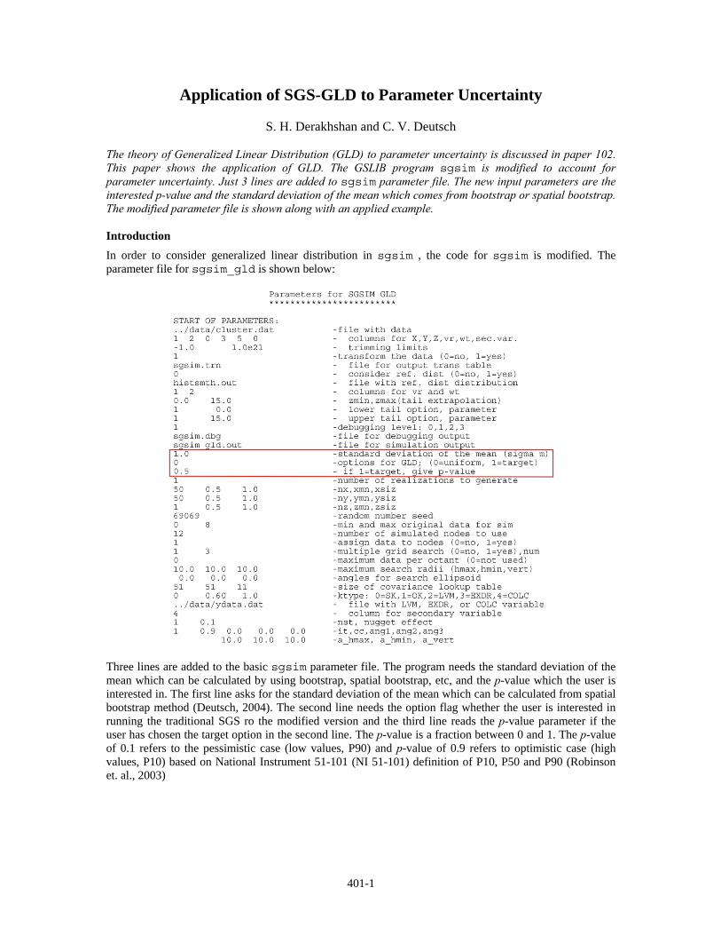
S. H. Derakhshan and C. V. Deutsch The theory of Generalized Linear Distribution (GLD) to parameter uncertainty is discussed in paper 102. This paper shows the application of GLD. The GSLIB program sgsim is modified to account for parameter uncertainty. Just 3 lines are added to sgsim parameter file. The new input parameters are the interested p-value and the standard deviation of the mean which comes from bootstrap or spatial bootstrap. The modified parameter file is shown along with an applied example. Introduction In order to consider generalized linear distribution in sgsim , the code for sgsim is modified. The parameter file for sgsim_gld is shown below:

Three lines are added to the basic sgsim parameter file. The program needs the standard deviation of the mean which can be calculated by using bootstrap, spatial bootstrap, etc, and the p-value which the user is interested in. The first line asks for the standard deviation of the mean which can be calculated from spatial bootstrap method (Deutsch, 2004). The second line needs the option flag whether the user is interested in running the traditional SGS ro the modified version and the third line reads the p-value parameter if the user has chosen the target option in the second line. The p-value is a fraction between 0 and 1. The p-value of 0.1 refers to the pessimistic case (low values, P90) and p-value of 0.9 refers to optimistic case (high values, P10) based on National Instrument 51-101 (NI 51-101) definition of P10, P50 and P90 (Robinson et. al., 2003)

401-2

Methodology

In this section the methodology which is used instead of uniform distribution to incorporate the GLD in sequential Gaussian simulation is presented along with an example. At first I should be calculated by using below formula.

( ){ } ( ) ( )2 1 2 1I E y F y y F y f y dy+∞

−∞⎡ ⎤ ⎡ ⎤= ⋅ − = ⋅ − ⋅ ⋅⎣ ⎦ ⎣ ⎦∫ ……...……………………...………...…….(1)

The only thing that we need to characterize the quantile function of standard GLD is η by using below equations.

( )1m my m G pI I

ση −− ⎛ ⎞= = ⋅⎜ ⎟

⎝ ⎠…………………………………………...……………………………….(2)

( ) ( )( )2

11 4 1

2p

q p F pη η η

η−

− + − += = ………………………...…………………………..……….(3)

The uniform distribution is replaced with this quantile function to draw from the Gaussian distribution in sequential Gaussian simulation procedure. The slope parameter η is calibrated according to the p-value which we want. To have high values in model, we need to have η close to 1 and to have low values in model η should be close to -1. The full theory and description is explained earlier in this annual report.

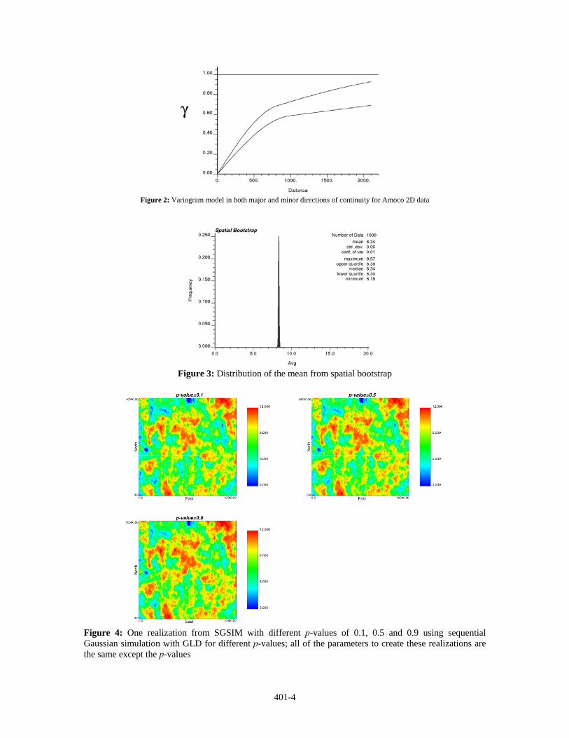
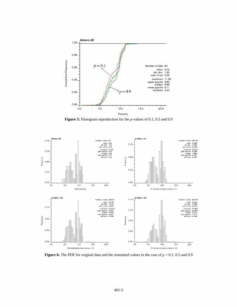
Example Amoco 2D data (Chu et al, 1995) is used to apply the methodology. Figure 1 shows the location, PDF and CDF of the Amoco 2D data. The variogram is calculated and modeled in both major and minor directions. The variogram model is illustrated in Figure 2. The spatial bootstrap is performed to get the standard deviation of the mean. Figure 3 shows the distribution of the mean from Spatial Bootstrap. The standard deviation of the mean is calculated and is equal to 0.06. I is calculated to be equal to 1.2204. Therefore the distribution of η is Gaussian with mean of zero and the standard deviation of σm/I. One realization is created using sequential Gaussian simulation with different p-values. It is obvious that small p-values lead to have a model with low values since we are interested to target the low mean value. Figure 4 shows the simulated field for 3 different p-values of 0.1, 0.5 and 0.9. The p-value of 0.1 shows more low values while the p-value of 0.9 shows more high values. The p-value of 0.5 shows the created realization from traditional sequential Gaussian simulation because the p-value of 0.5 gives the η parameter of zero and the zero η parameter converts the linear distribution to uniform distribution. Figure 5 and Figure 6 show the histogram reproduction for 3 different cases of targeted p-value or η parameter. Small p-value corresponds to small negative η parameter and it causes to draw small values from the Gaussian distribution. In the case of high p-values; because of high positive η parameters the Monte Carlo method is forced to draw the high values. In the case of targeted p-value, the global mean, global standard deviation and global coefficient of variation of the simulated field are calculated for each specific p-value. The plots of these variables versus the p-value are shown in Figure 7. As we expect the distribution of calculated global mean follows the Gaussian distribution because of Central Limit Theorem. The variogram reproduction is also checked for different cases. Figure 8 shows the variogram reproduction for the cases with p-values of 0.1, 0.5 and 0.9. There are not big changes in the calculated variogram. Although these three different variograms are coincided each other but there are some minor differences in calculated variograms. High p-values will cause decreasing the variogram range in minor direction and increasing the variogram range in major direction but these increase or decrease are minor. It is mainly due to the narrow distribution that η parameter has.

401-3

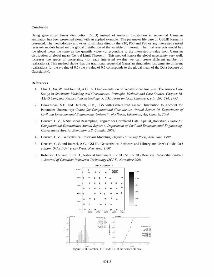
Conclusion Using generalized linear distribution (GLD) instead of uniform distribution in sequential Gaussian simulation has been presented along with an applied example. The parameter file base on GSLIB format is presented. The methodology allows us to simulate directly the P10, P50 and P90 or any interested ranked reservoir models based on the global distribution of the variable of interest. The final reservoir model has the global mean the same as the quantile value corresponding to the interested p-value from Gaussian distribution of global mean (Central Limit Theorem). This method honors the global uncertainty very well, increases the space of uncertainty (for each interested p-value we can create different number of realizations). This method shows that the traditional sequential Gaussian simulation just generate different realizations for the p-value of 0.5 (the p-value of 0.5 corresponds to the global mean of the Data because of Gaussianity).

References

1. Chu, J., Xu, W. and Journel, A.G., 3-D Implementation of Geostatistical Analyses: The Amoco Case Study; In Stochastic Modeling and Geostatistics: Principle, Methods and Case Studies, Chapter 16, AAPG Computer Applications in Geology, 3, J.M. Yarus and R.L. Chambers, eds., 201-216, 1995.

2. Derakhshan, S.H. and Deutsch, C.V., SGS with Generalized Linear Distribution to Account for Parameter Uncertainty; Centre for Computational Geostatistics Annual Report 10, Department of Civil and Environmental Engineering, University of Alberta, Edmonton, AB, Canada, 2008.

3. Deutsch, C.V., A Statistical Resampling Program for Correlated Data : Spatial_Bootstrap; Centre for Computational Geostatistics Annual Report 6, Department of Civil and Environmental Engineering, University of Alberta, Edmonton, AB, Canada, 2004.

4. Deutsch, C.V., Geostatistical Reservoir Modeling; Oxford University Press, New York, 1998.

5. Deutsch, C.V. and Journel, A.G., GSLIB: Geostatistical Software and Library and User's Guide; 2nd edition, Oxford University Press, New York, 1998.

6. Robinson J.G. and Elliot D., National Instrument 51-101 (NI 51-101) Reserves Reconciliation-Part 1, Journal of Canadian Petroleum Technology (JCPT), November 2004.

Figure 1: The location, PDF and CDF of the Amoco 2D data

401-4

Figure 2: Variogram model in both major and minor directions of continuity for Amoco 2D data

Figure 3: Distribution of the mean from spatial bootstrap

Figure 4: One realization from SGSIM with different p-values of 0.1, 0.5 and 0.9 using sequential Gaussian simulation with GLD for different p-values; all of the parameters to create these realizations are the same except the p-values

401-5

Figure 5: Histogram reproduction for the p-values of 0.1, 0.5 and 0.9

Figure 6: The PDF for original data and the simulated values in the case of p = 0.1, 0.5 and 0.9

F

Figure 7: Calccoefficie

Figu

ulated global ment of variation

ure 8: Variogra

mean (top figurn (bottom right)

am reproductio

401-6

re), global stan) for each simu

on for different

ndard deviationulated field for

t p-values of 0

n (bottom left) r different p-va

.1, 0.5 and 0.9

and global alues