application of statistical learning theory to plankton
TRANSCRIPT
Application of Statistical Learning Theory to
Plankton Image Analysisby
Qiao HuB.S., University of Science and Technology of China(1990)M.S., University of Science and Technology of China(1993)
Submitted to the Joint Program in Applied Ocean Science and
Engineeringin partial fulfillment of the requirements for the degree of
Doctor of Philosophyat the
MASSACHUSETTS INSTITUTE OF TECHNOLOGYand the
WOODS HOLE OCEANOGRAPHIC INSTITUTIONJune 2006
c©Woods Hole Oceanographic Institution 2006. All rights reserved.
Author . . . . . . . . . . . . . . . . . . . . . . . . . . . . . . . . . . . . . . . . . . . . . . . . . . . . . . . . . . . . . .
Joint Program in Applied Ocean Science and EngineeringApril 25, 2006
Certified by. . . . . . . . . . . . . . . . . . . . . . . . . . . . . . . . . . . . . . . . . . . . . . . . . . . . . . . . . .
Cabell S. DavisSenior Scientist, WHOI
Thesis Supervisor
Certified by. . . . . . . . . . . . . . . . . . . . . . . . . . . . . . . . . . . . . . . . . . . . . . . . . . . . . . . . . .Hanumant Singh
Associate Scientist, WHOIThesis Supervisor
Accepted by . . . . . . . . . . . . . . . . . . . . . . . . . . . . . . . . . . . . . . . . . . . . . . . . . . . . . . . . .Henrik Schmidt
Chairman, Joint Committee for Applied Ocean Science andEngineering
Accepted by . . . . . . . . . . . . . . . . . . . . . . . . . . . . . . . . . . . . . . . . . . . . . . . . . . . . . . . . .
Lallit AnandChairman, Committee on Graduate Student, Department of
Mechanical Engineering

2

Application of Statistical Learning Theory to Plankton
Image Analysis
by
Qiao Hu
Submitted to the Joint Program in Applied Ocean Science and Engineeringon April 25, 2006, in partial fulfillment of the
requirements for the degree ofDoctor of Philosophy
Abstract
A fundamental problem in limnology and oceanography is the inability to quicklyidentify and map distributions of plankton. This thesis addresses the problem byapplying statistical machine learning to video images collected by an optical sam-pler, the Video Plankton Recorder (VPR). The research is focused on developmentof a real-time automatic plankton recognition system to estimate plankton abun-dance. The system includes four major components: pattern representation/featuremeasurement, feature extraction/selection, classification, and abundance estimation.
After an extensive study on a traditional learning vector quantization (LVQ)neural network (NN) classifier built on shape-based features and different patternrepresentation methods, I developed a classification system combined multi-scale co-occurrence matrices feature with support vector machine classifier. This new methodoutperforms the traditional shape-based-NN classifier method by 12% in classificationaccuracy. Subsequent plankton abundance estimates are improved in the regions oflow relative abundance by more than 50%.
Both the NN and SVM classifiers have no rejection metrics. In this thesis, tworejection metrics were developed. One was based on the Euclidean distance in thefeature space for NN classifier. The other used dual classifier (NN and SVM) voting asoutput. Using the dual-classification method alone yields almost as good abundanceestimation as human labeling on a test-bed of real world data. However, the distancerejection metric for NN classifier might be more useful when the training samples arenot “good” ie, representative of the field data.
In summary, this thesis advances the current state-of-the-art plankton recogni-tion system by demonstrating multi-scale texture-based features are more suitablefor classifying field-collected images. The system was verified on a very large real-world dataset in systematic way for the first time. The accomplishments includedeveloping a multi-scale occurrence matrices and support vector machine system, adual-classification system, automatic correction in abundance estimation, and abilityto get accurate abundance estimation from real-time automatic classification. The
3

methods developed are generic and are likely to work on range of other image classi-fication applications.
Thesis Supervisor: Cabell S. DavisTitle: Senior Scientist, WHOI
Thesis Supervisor: Hanumant SinghTitle: Associate Scientist, WHOI
4

Acknowledgments
First of all, I would like to thank my co-advisors, Cabell Davis and Hanumant Singh.
They stand on my side with only occasional doubts. Even when I seemed have no
way out. Cabell Davis was always there when I needed his guidance. His enthusiasm
and “hands-on” approaches to science, both in the lab and during cruises, have been
an inspiration to me. He is a great scientist and a good mentor. Hanumant Singh
kept me on the track. He provided me the opportunity to share my work with fellow
students. He is a really expert on underwater imaging.
I would like to thank the rest of my committee members, Jerome Milgram and
George Barbastathis for their suggestions and useful criticism. I would like thank
Carin Ashjian for serving as chair of my defense.
This work was supported by National Science Foundation Grants OCE-9820099
and Woods Hole Oceanographic Institution academic program.
I would like thank Marine Ecology Progress Series for publishing my thesis Chapter
5 and 6 and giving me permission to include them in my thesis. Thanks to editors to
make these two chapters more readable.
I would like thank everyone in the Video Plankton Recorder group. Cabell Davis,
Scott Gallager, Carin Ashjian, Xiaoou Tang, Philip Alatalo, Andrew Girard and all
the others collected the images I used in my thesis. Cabell Davis and Philip Alatalo
taught me how to classify these images manually.
I would like thank everyone in Seabed AUV group. Hanumant Singh, Oscar
Pizarro, Ryan Eustice, Christopher Roman, Michael Jakuba and Anna Michel gave
me lots of comments and suggestions on my thesis work.
I would like thank everyone at WHOI Academic programs office. John Farrington,
Judith McDowell, Julia Westerwater, Marsha Gomes and Stacey Brudno Drange
made my long journey so wonderful and enjoyable.
I would like thank everyone who are kind enough to read my thesis draft. Judith
Fenwick, Colleen Petrik, Gareth Lawson and Sanjay Tiwari read part or whole thesis.
I would like thank all my friends: Xiaoou Tang, Guangyu Wu, Weichang Li,
5

Wenyu Luo and Jinshan Xu, Zao Xu and Gareth Lawson. I had such a memorable
time with them.
Last but not least, I would like thank my family. My wife Xingwen Li and my
daughter Daisy Xuyuan Hu make such a warmth home for me. Their love, constant
support and confidence gave me the great strength to break through all the difficulties.
I thank my parents and my sisters for their understanding and patience.
6

Contents
1 Introduction 25
1.1 Motivation . . . . . . . . . . . . . . . . . . . . . . . . . . . . . . . . . 26
1.2 Statistical pattern recognition . . . . . . . . . . . . . . . . . . . . . . 26
1.2.1 Features . . . . . . . . . . . . . . . . . . . . . . . . . . . . . . 27
1.2.2 Statistical learning theory . . . . . . . . . . . . . . . . . . . . 29
1.3 An overview of related work . . . . . . . . . . . . . . . . . . . . . . . 30
1.4 Data . . . . . . . . . . . . . . . . . . . . . . . . . . . . . . . . . . . . 32
1.5 Thesis overview . . . . . . . . . . . . . . . . . . . . . . . . . . . . . . 33
2 Data Acquisition 39
2.1 Water column plankton samplers . . . . . . . . . . . . . . . . . . . . 39
2.2 Video Plankton Recorder . . . . . . . . . . . . . . . . . . . . . . . . . 42
2.3 Focus Detection . . . . . . . . . . . . . . . . . . . . . . . . . . . . . . 44
2.3.1 Objective . . . . . . . . . . . . . . . . . . . . . . . . . . . . . 44
2.3.2 Method . . . . . . . . . . . . . . . . . . . . . . . . . . . . . . 46
2.3.3 Algorithms . . . . . . . . . . . . . . . . . . . . . . . . . . . . 47
2.3.4 Result . . . . . . . . . . . . . . . . . . . . . . . . . . . . . . . 48
2.4 Conclusion . . . . . . . . . . . . . . . . . . . . . . . . . . . . . . . . . 52
3 Classification Method: Analysis and Assessment 53
3.1 System overview . . . . . . . . . . . . . . . . . . . . . . . . . . . . . 54
3.1.1 Artificial Neural Networks . . . . . . . . . . . . . . . . . . . . 54
3.1.2 Learning vector quantization neural network classifier . . . . . 54
7

3.1.3 Principal component analysis . . . . . . . . . . . . . . . . . . 55
3.1.4 Feature extraction . . . . . . . . . . . . . . . . . . . . . . . . 56
3.1.5 Classification performance estimation . . . . . . . . . . . . . . 56
3.2 Assessment Result . . . . . . . . . . . . . . . . . . . . . . . . . . . . 58
3.2.1 Classifier complexity vs. classifier performance . . . . . . . . . 58
3.2.2 Feature length versus classification performance . . . . . . . . 58
3.2.3 Learning curve - numbers of training samples versus classifier
performance . . . . . . . . . . . . . . . . . . . . . . . . . . . . 60
3.2.4 Initial neuron position versus presentation order of training
samples . . . . . . . . . . . . . . . . . . . . . . . . . . . . . . 63
3.2.5 Training samples effect . . . . . . . . . . . . . . . . . . . . . . 64
3.2.6 Classification stability . . . . . . . . . . . . . . . . . . . . . . 65
3.3 Two-pass classification system . . . . . . . . . . . . . . . . . . . . . . 66
3.3.1 Decision rules . . . . . . . . . . . . . . . . . . . . . . . . . . . 68
3.3.2 Implementation . . . . . . . . . . . . . . . . . . . . . . . . . . 71
3.3.3 Results . . . . . . . . . . . . . . . . . . . . . . . . . . . . . . . 71
3.3.4 Discussion . . . . . . . . . . . . . . . . . . . . . . . . . . . . . 73
3.4 Statistical correction method . . . . . . . . . . . . . . . . . . . . . . . 75
3.4.1 Method . . . . . . . . . . . . . . . . . . . . . . . . . . . . . . 75
3.4.2 Result . . . . . . . . . . . . . . . . . . . . . . . . . . . . . . . 76
3.5 Distance rejection metric for LVQ-NN classifier . . . . . . . . . . . . 77
3.5.1 Distance rejection system . . . . . . . . . . . . . . . . . . . . 78
3.5.2 Result and discussion . . . . . . . . . . . . . . . . . . . . . . . 78
3.6 Conclusion . . . . . . . . . . . . . . . . . . . . . . . . . . . . . . . . . 83
4 Pattern Representation/Feature Measurement 85
4.1 Pattern representation methods . . . . . . . . . . . . . . . . . . . . . 86
4.1.1 Shape-based methods . . . . . . . . . . . . . . . . . . . . . . . 86
4.1.2 Texture-based methods . . . . . . . . . . . . . . . . . . . . . . 90
4.1.3 Other Methods . . . . . . . . . . . . . . . . . . . . . . . . . . 95
8

4.2 Feature extraction and classification . . . . . . . . . . . . . . . . . . . 97
4.3 Results and discussion . . . . . . . . . . . . . . . . . . . . . . . . . . 100
4.3.1 High order moment invariants . . . . . . . . . . . . . . . . . . 103
4.3.2 Radial Fourier descriptors vs. complex Fourier descriptors . . 105
4.3.3 Co-occurrence matrices . . . . . . . . . . . . . . . . . . . . . . 107
4.3.4 Edge frequency . . . . . . . . . . . . . . . . . . . . . . . . . . 110
4.3.5 Run length . . . . . . . . . . . . . . . . . . . . . . . . . . . . 111
4.3.6 Pattern spectrum . . . . . . . . . . . . . . . . . . . . . . . . . 112
4.3.7 Wavelet transform . . . . . . . . . . . . . . . . . . . . . . . . 112
4.4 Conclusion . . . . . . . . . . . . . . . . . . . . . . . . . . . . . . . . . 114
5 Co-Occurrence Matrices and Support Vector Machine 115
5.1 Co-Occurrence Matrices . . . . . . . . . . . . . . . . . . . . . . . . . 116
5.2 Support Vector Machines . . . . . . . . . . . . . . . . . . . . . . . . . 116
5.3 Feature Extraction and Classification . . . . . . . . . . . . . . . . . . 118
5.4 Classification results . . . . . . . . . . . . . . . . . . . . . . . . . . . 119
5.5 Conclusion . . . . . . . . . . . . . . . . . . . . . . . . . . . . . . . . . 126
6 Dual classification system and accurate plankton abundance estima-
tion 129
6.1 Dual classification system description . . . . . . . . . . . . . . . . . . 130
6.1.1 Pattern representations . . . . . . . . . . . . . . . . . . . . . . 130
6.1.2 Feature extraction . . . . . . . . . . . . . . . . . . . . . . . . 132
6.1.3 Classifiers . . . . . . . . . . . . . . . . . . . . . . . . . . . . . 133
6.1.4 Dual classification system . . . . . . . . . . . . . . . . . . . . 134
6.1.5 Classification performance evaluation and abundance correction 136
6.2 Classification results . . . . . . . . . . . . . . . . . . . . . . . . . . . 138
6.3 Conclusion . . . . . . . . . . . . . . . . . . . . . . . . . . . . . . . . . 147
7 Conclusions and future work 149
7.1 Summary of major contributions . . . . . . . . . . . . . . . . . . . . 150
9

7.2 Future research directions . . . . . . . . . . . . . . . . . . . . . . . . 153
10
List of Figures
1-1 Schematic diagram of the pattern recognition system. . . . . . . . . . . . 28
1-2 Example VPR images of copepods, rod-shaped diatom chain, Chaetoceros
socialis colonies and the “other” category. Fifty randomly selected samples
are shown here. . . . . . . . . . . . . . . . . . . . . . . . . . . . . . . 34
1-3 Example VPR images of Chaetoceros chains and marine snow. Fifty ran-
domly selected samples are shown here. . . . . . . . . . . . . . . . . . . 35
1-4 Example VPR images of hydroid medusae. Fifty randomly selected samples
are shown here. . . . . . . . . . . . . . . . . . . . . . . . . . . . . . . . 36
2-1 Video Plankton Recorder system with underwater and shipboard compo-
nents. The VPR is towyoed at ship speeds up to 5 m/s, while video is
processed in real-time on board. . . . . . . . . . . . . . . . . . . . . . . 43
2-2 The graphical user interface of real time focus detection program. . . . . . 45
3-1 Classification performance with respect to classifier complexity. . . . . 59
3-2 Training and test accuracy with respect to classifier complexity. . . . 59
3-3 Classification performance as a function of feature length for each taxon. 60
3-4 Training and test accuracy with respect to feature length. . . . . . . . 61
3-5 Classification performance as a function of training sample size for each
taxon. . . . . . . . . . . . . . . . . . . . . . . . . . . . . . . . . . . . 62
3-6 Training and test accuracy with respect to training sample size. . . . 63
11
3-7 Comparison between the random initial position of neurons and ran-
dom order of presentation order of training samples. IP1 - different
initial position of neurons, random representation order of training
samples; IP2 - same initial position of neurons, random representation
order of training samples . . . . . . . . . . . . . . . . . . . . . . . . . 64
3-8 Comparison of different training samples effect on classfication perfor-
mance. TS1 - different sets of training samples, leave-one-out method;
TS2 - different sets of training samples, holdout method; TS3 - single
set training samples, holdout method . . . . . . . . . . . . . . . . . . 66
3-9 Mean, upper and lower limit of 95% confidence interval of abundance
estimates from LVQ-NN classifiers and that of manually sorted results.
Time series abundance plots along the tow path are shown for 6 dom-
inant taxa. Data were first binned in 10 second time intervals, and a
one-hour smoothing window was applied to the binned data. . . . . . 67
3-10 Illustration of the three most popular decision rules. x∗ML - maximum
likelihood decision rule, x∗MAP - maximum a posteriori decision rule,
x∗MM - minimax decision rule . . . . . . . . . . . . . . . . . . . . . . . 70
3-11 Schematic diagram of two pass classification system . . . . . . . . . . 72
3-12 Comparison of two automatic classification systems with human expert
classified results. Time series abundance plots along the tow path are
shown for 6 dominant taxa. Data were first binned in 10 second time
intervals, and a one-hour smoothing window was applied to the binned
data. . . . . . . . . . . . . . . . . . . . . . . . . . . . . . . . . . . . . 74
3-13 Comparison of automatic classification systems with/without statisti-
cal correction to human expert classified results. Time series abun-
dance plots along the tow path are shown for 6 dominant taxa. Data
were first binned in 10 second time intervals, and a one-hour smoothing
window was applied to the binned data. . . . . . . . . . . . . . . . . 77
3-14 Schematic diagram of distance rejection classification system . . . . . 79
12
4-1 Mean and standard deviation of classification accuracy from different
feature presentation methods for each taxon. The abbreviations are as
follows: MI - moment invariants, FD - Fourier descriptors, SS - shape
spectrum, MM - morphological measurements, CM - co-occurrence ma-
trices, RL - run length, EF - edge frequency, PS - pattern spectrum,
WT - wavelet transform. It clearly shows the jump between shape-
based features and texture-based features. The pattern spectrum and
wavelet transform methods are between shape-based and texture-based
methods, their performances lie in between these two group of methods.102
4-2 Illustrates the problem of non-uniform illunimation on segmentation.
(a) the original image, (b) gradient correction of (a), (c) segmentation
of (a), (d) segmentation of (b), (e) contour of the largest object from
(c), (f) contour of the largest object from (d) . . . . . . . . . . . . . . 104
4-3 Mean and standard deviation of classification accuracy for moment
invariants of different orders for each taxon. MI3-7 stands for moment
invariants up to order 3-7, which correspond to feature length of 7, 12,
18, 24, and 33 respectively. where MI3 is equivalent to Hu’s moment
invariants. There is no benefit to using high order moment invariants
in this dataset. . . . . . . . . . . . . . . . . . . . . . . . . . . . . . . 105
4-4 Illustrates the problem of using a radius-vector function to encode a
non-star-shaped plankton image. (a) the original image, (b) the con-
tour of the object, (c) the radius-vector function from the contour
model of (b), (d) the recovered contour of the object based on radius-
vector function (c) with assumption that the object is star-shaped. . . 106
4-5 A comparison between radial Fourier descriptors (RFD) and complex
Fourier descriptors (CFD). . . . . . . . . . . . . . . . . . . . . . . . . 107
13
4-6 Mean and standard deviation of classification accuracy for co-occurrence
matrices of different multi-scale levels for each taxon. The abbrevia-
tions CM1-6 stand for co-occurrence matrices of multi-scale levels from
1 to 6, which correspond to feature length of 16, 32, 48, 64, 80, and
96 respectively. The classification accuracy first rises sharply with an
increase of multi-scale levels, and reaches top performance with 3-4
multi-scale levels. The performance then drops down slightly as more
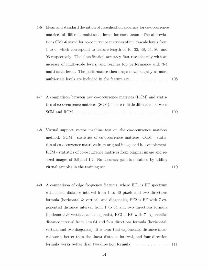
multi-scale levels are included in the feature set. . . . . . . . . . . . . 108
4-7 A comparison between raw co-occurrence matrices (RCM) and statis-
tics of co-occurrence matrices (SCM). There is little difference between
SCM and RCM. . . . . . . . . . . . . . . . . . . . . . . . . . . . . . . 109
4-8 Virtual support vector machine test on the co-occurrence matrices
method. SCM - statistics of co-occurrence matrices, CCM - statis-
tics of co-occurrence matrices from original image and its complement,
RCM - statistics of co-occurrence matrices from original image and re-
sized images of 0.8 and 1.2. No accuracy gain is obtained by adding
virtual samples in the training set. . . . . . . . . . . . . . . . . . . . 110
4-9 A comparison of edge frequency features, where EF1 is EF spectrum
with linear distance interval from 1 to 40 pixels and two directions
formula (horizontal & vertical, and diagonals), EF2 is EF with 7 ex-
ponential distance interval from 1 to 64 and two directions formula
(horizontal & vertical, and diagonals), EF3 is EF with 7 exponential
distance interval from 1 to 64 and four directions formula (horizontal,
vertical and two diagonals). It is clear that exponential distance inter-
val works better than the linear distance interval, and four direction
formula works better than two direction formula. . . . . . . . . . . . 111
14
4-10 Comparison of run length methods. RL1 - run length statistics pro-
posed by Galloway, 5 statistics from each run length matrix, total 20
features for 4 directions. RL2 - extended run length statisitcs by Chu
et al., and by Dasarathy and Holder. 11 statistics from each run length
matrix, total 44 features for 4 directions. The extended features give
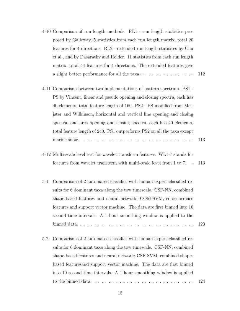
a slight better performance for all the taxa. . . . . . . . . . . . . . . . 112
4-11 Comparison between two implementations of pattern spectrum. PS1 -
PS by Vincent, linear and pseudo opening and closing spectra, each has
40 elements, total feature length of 160. PS2 - PS modified from Mei-
jster and Wilkinson, horizontal and vertical line opening and closing
spectra, and area opening and closing spectra, each has 40 elements,
total feature length of 240. PS1 outperforms PS2 on all the taxa except
marine snow. . . . . . . . . . . . . . . . . . . . . . . . . . . . . . . . 113
4-12 Multi-scale level test for wavelet transform features. WL1-7 stands for
features from wavelet transform with multi-scale level from 1 to 7. . 113
5-1 Comparison of 2 automated classifier with human expert classified re-
sults for 6 dominant taxa along the tow timescale. CSF-NN, combined
shape-based features and neural network; COM-SVM, co-occurrence
features and support vector machine. The data are first binned into 10
second time intervals. A 1 hour smoothing window is applied to the
binned data. . . . . . . . . . . . . . . . . . . . . . . . . . . . . . . . . 123
5-2 Comparison of 2 automated classifier with human expert classified re-
sults for 6 dominant taxa along the tow timescale. CSF-NN, combined
shape-based features and neural network; CSF-SVM, combined shape-
based featuresand support vector machine. The data are first binned
into 10 second time intervals. A 1 hour smoothing window is applied
to the binned data. . . . . . . . . . . . . . . . . . . . . . . . . . . . . 124
15

5-3 Reduction in the relative abundance estimation error rate between
COM-SVM and CSF-NN, and between CSF-SVM and CSF-NN. The
positive value indicates that COM-SVM/CSF-SVM is better than CSF-
NN, while the negative value indicates COM-SVM/CSF-NN is worse
than CSF-NN. . . . . . . . . . . . . . . . . . . . . . . . . . . . . . . . 125
6-1 Schematic diagram of dual-classification system. LVQ: learning vector
quantization; NN: neural netowork; SVM: support vector machine . . 135
6-2 Automatically classified images: comparison of results for(A,C) dual-
classification system and (B,D) single neural network classifier. The
first 25 images classified as (A,B) copepods and (C,D) Chaetoceros
socialis by the dual-classification system and LVQ-NN classifier are
shown. For taxa having relatively high abundance, such as copepods,
both systems yield very similar results (21 out of 25 were the same).
In contrast, for taxa having relatively low abundance, such as low-
abundance regions of C. socialis, the dual-classification system has
much higher specificity (fewer false alarms). . . . . . . . . . . . . . . 139
6-3 Comparison of dual-classification, and manually corrected single NN
classification with human expert classified results for 6 dominant taxa
along the tow timescale. The data are first binned into 10 second time
intervals. A 1 hour smoothing window is applied to the binned data. . 141
6-4 Comparison of 3 automated classifier with human expert classified re-
sults for 6 dominant taxa along the tow timescale. CSF-NN, combined
shape-based features and neural network; CSF-SVM, combined shape-
based features and support vector machine. The data are first binned
into 10 second time intervals. A 1 hour smoothing window is applied
to the binned data. . . . . . . . . . . . . . . . . . . . . . . . . . . . . 143
16
6-5 Reduction in error rate between the dual- and single-classification sys-
tems for relative abundance estimation. Positive values indicate that
the dual-classification outperforms other methods; negative values in-
dicate the opposite. Dual: dual-classification system, CSF-NN: com-
bined shape-based features and neural network; CSF-SVM, combined
shape-based features and support vector machine. . . . . . . . . . . . 145
6-6 Relationship between specificity and relative abundance for different
false alarm rates. Probability of detection is set to 70%. As false
alarm rates become smaller, the range in which the specificity closes
to a constant becomes wider. The dual-classification system has sub-
stantially reduced the false alarm rates, so that the specificity of each
taxon in the whole study area is close to a constant. This makes fully
automatic correction possible. . . . . . . . . . . . . . . . . . . . . . . 146
17

18

List of Tables
2.1 Comparison of focus detection algorithms from AN9703, high magni-
fication camera, video section 1. The numbers are blob counts; prob-
ability of detection Pd and probability of false alarm Pf are given as
percentages. . . . . . . . . . . . . . . . . . . . . . . . . . . . . . . . . 49
2.2 Comparison of focus detection algorithms from AN9703, high magni-
fication camera, video section 2. The numbers are blob counts; prob-
ability of detection Pd and probability of false alarm Pf are given as
percentages. . . . . . . . . . . . . . . . . . . . . . . . . . . . . . . . . 49
2.3 Comparison of focus detection algorithms from AN9703, high magnifi-
cation camera, video section 1 after correction. The numbers are blob
counts; probability of detection Pd and probability of false alarm Pf
are given as percentages. . . . . . . . . . . . . . . . . . . . . . . . . . 50
2.4 Comparison of focus detection algorithms from AN9703, high magnifi-
cation camera, video section 2 after correction. The numbers are blob
counts; probability of detection Pd and probability of false alarm Pf
are given as percentages. . . . . . . . . . . . . . . . . . . . . . . . . . 51
2.5 Comparison of focus detection algorithms from HALOS, low magni-
fication camera, video section 1. The numbers are the blob counts;
probability of detection Pd and probability of false alarm Pf are given
as percentages. . . . . . . . . . . . . . . . . . . . . . . . . . . . . . . 52
19

2.6 Comparison of focus detection algorithms from HALOS, low magni-
fication camera, video section 2. The numbers are the blob counts;
probability of detection Pd and probability of false alarm Pf are given
as percentages. . . . . . . . . . . . . . . . . . . . . . . . . . . . . . . 52
3.1 Confusion matrix of an LVQ-NN classifier with distance rejection met-
ric using hold-out method. The classifier was trained without marine
snow. Column and row heading are coded as: C1, copepod; C2, rod-
shaped diatom chains; C3, Chaetoceros chains; C4, Chaetoceros socialis
colonies; C5, hydroid medusae; C6, marine snow; C6*, “unknown”. . 80
3.2 Confusion matrix of an LVQ-NN classifier with distance rejection met-
ric using hold-out method. The classifier was trained without hydroid
medusae. Column and row heading are coded as: C1, copepod; C2,
rod-shaped diatom chains; C3, Chaetoceros chains; C4, Chaetoceros so-
cialis colonies; C5, marine snow; C6, hydroid medusae; C6*, “unknown”. 81
3.3 Confusion matrix of an LVQ-NN classifier with distance rejection met-
ric using hold-out method. The classifier was trained without Chaeto-
ceros socialos colonies. Column and row heading are coded as: C1,
copepod; C2, rod-shaped diatom chains; C3, Chaetoceros chains; C4,
hydroid medusae; C5, marine snow; C6, Chaetoceros socialis colonies;
C6*, “unknown”. . . . . . . . . . . . . . . . . . . . . . . . . . . . . . 81
3.4 Confusion matrix of an LVQ-NN classifier with distance rejection met-
ric using hold-out method. The classifier was trained without Chaeto-
ceros chains. Column and row heading are coded as: C1, copepod;
C2, rod-shaped diatom chains; C3, Chaetoceros socialos colonies; C4,
hydroid medusae; C5, marine snow; C6, Chaetoceros chains; C6*, “un-
known”. . . . . . . . . . . . . . . . . . . . . . . . . . . . . . . . . . . 81
20
3.5 Confusion matrix of an LVQ-NN classifier with distance rejection met-
ric using hold-out method. The classifier was trained without rod-
shaped diatom chains. Column and row heading are coded as: C1,
copepod; C2, Chaetoceros chains; C3, Chaetoceros socialis colonies;
C4, hydroid medusae; C5, marine snow; C6, rod-shaped diatom chains;
C6*, “unknown”. . . . . . . . . . . . . . . . . . . . . . . . . . . . . . 82
3.6 Confusion matrix of an LVQ-NN classifier with distance rejection met-
ric using hold-out method. The classifier was trained without copepod.
Column and row heading are coded as: C1, rod-shaped diatom chains;
C2, Chaetoceros chains; C3, Chaetoceros socialis colonies; C4, hydroid
medusae; C5, marine snow; C6, copepod; C6*, “unknown”. . . . . . . 82
4.1 Mean classification accuracy from different feature representation meth-
ods, where the unit is in percent. The abbreviations are as follows: MI
- moment invariants, FD - Fourier descriptors, SS - shape spectrum,
MM - morphological measurements, CM - co-occurrence matrices, RL -
run length, EF - edge frequency, PS - pattern spectrum, WT - wavelet
transform. The best performance for single feature method is the co-
occurrence matrices method, which has the average of classification
accuracy of 74%. It is clear to see that the texture-based methods are
superior than shape-based methods. . . . . . . . . . . . . . . . . . . . 101
4.2 Standard deviation of classification rates from different feature repre-
sentation methods, where the unit is in percent. The abbreviations are
same as Table 4.1. . . . . . . . . . . . . . . . . . . . . . . . . . . . . 101
21

5.1 Confusion matrix for EN302, VPR Tow 7, based on the co-occurence
matrix classifier using hold-out method. Column and row heading are
coded as: C1, copepod; C2, rod-shaped diatom chains; C3, Chaeto-
ceros chains; C4, Chaetoceros socialis colonies; C5, hydroid medusae;
C6, marine snow; C7, ’other’; and Pd, probability of detection. True
counts (i.e. human counts) for a given taxa are given in the columns,
while counts by automatic identification (i.e. computer counts) are
given in the rows. Correct identifications by the computer are given
along the main diagonal, while the off-diagonal entries are the incorrect
identification by the computer. Overall accuracy for this classifier was
72%. . . . . . . . . . . . . . . . . . . . . . . . . . . . . . . . . . . . . 120
5.2 Mean confusion matrix for EN302, VPR Tow 7, based on learning
vector quatization method neural network classifiers built with different
randomly selected sets of 200 training ROIs using hold-out method
[34]. Column and row headings are as in Table 5.1. True counts (i.e.
human counts) for a given taxa are given in the columns, while counts
by attomatic identification (i.e. computer counts) are given in the rows.
The correct identifications by the computer are given along the main
diagonal, while the off-diagonal entries are the incorrect identification
by the computer. Overall accuracy of this classifier was 61%. . . . . . 121
5.3 Performance of the classifier with different kernel widths (σ), regulation
penalty (C) and kernel types, where d is the polynomial degree and κ
is the kernel coefficient. The recognition rate on the independent test
set is shown. . . . . . . . . . . . . . . . . . . . . . . . . . . . . . . . . 122
5.4 Kullback-Leibler(KL) distance estimation for difference in abundance
between COM-SVM and hand-sorted and between CSF-NN and hand-
sorted. Row headings are as in Table 5.1. The KL distance is dimen-
sionless. For two identical abundance curves, the KL distance is 0,
while for two random distributions, the KL distance is 0.5. Note lower
values of COM-SVM than CSF-NN for all four taxa. . . . . . . . . . 124
22

6.1 Confusion matrix of the dual-classification system, using the leave-one-
out method. Randomly selected images (200 per category) from EN302
VPR tow 7 were used to build the confusion matrix. C1: copepods, C2:
rod-shaped diatom chains, C3: Chaetoceros chains, C4: Chaetoceros
socialis colonies, C5: hydroid medusae, C6: marine snow, C7: other,
C7*: unknown, PD: probability of detection (%), SP = specificity
(%). NA: not applicable. True counts (i.e. human counts) for a given
taxa are given in the columns, while counts by classification system are
given in the rows. Correct identifications by the computer are given
along the main diagonal, while the off-diagonal entries are the incorrect
identification by the computer. All data are counts, except in the last
row and last column, which are percent values. Although images from
the “other” category are not needed to train the dual-classification
system, they are necessary to evaluate it. . . . . . . . . . . . . . . . . 137
6.2 Confusion matrix of the single LVQ-NN classifier, using the leave-one-
out method. Images used were the same as those in Table 6.1. Ab-
breviations as in Table 6.1. All data are counts, except in the last row
and last column, which are percent values. . . . . . . . . . . . . . . . 140
23

24

Chapter 1
Introduction
The vast majority of species in the ocean are plankton. The term plankton was
coined by the German scientist Victor Henson at the University of Kiel in 1887 from
the Greek word “planktos”, meaning “drifter”, to describe the passively drifting or-
ganisms in freshwater and marine ecosystems. Many species are planktonic for only
part of their lives (meroplankton), including larvae of fish, crabs, starfish, mollusks,
corals, etc. Other species are always planktonic (holoplankton), including the many
species of phytoplankton and copepods. As primary producers, phytoplankton are
responsible for approximately 40% of the annual photosynthetic production on earth.
Phytoplankton and their predators, zooplankton, play important roles in processes
such as the carbon cycle, the biological pump, global warming, harmful algal blooms
and coastal eutrophication. As the base of the ocean food web, plankton play impor-
tant roles in sustaining commercial marine fisheries. In order to better understand
the marine ecosystem, knowledge of the size structure, abundance, mass, and species
composition of plankton is crucial. Such measurements are difficult however, since
plankton distributions are notoriously patchy and require high-resolution sampling
tools for adequate quantification [45, 61, 120, 108]. In spite of over a hundred years
of research [168], our understanding of the structure of aggregations of plankton is
still very limited. Taxa-specific abundance at both fine-scale temporal and spatial
resolution is necessary to assess theoretical ecological models such as those of Riley
[134], Fasham [46], Aksnes et al. [2], Lynch et al. [107], Miller et al. [115], and
25
Carlotti et al. [17].
1.1 Motivation
The advent of new optical imaging sampling systems [31] in the last two decades offers
an opportunity to resolve taxa-specifc plankton distribution at much higher spatial
and temporal resolution than previously possible with net, pump, and bottle collec-
tions. Optical imaging systems rapidly create large amounts of digital image data and
ancillary environmental data that need to be analyzed and interpreted. Analyzing
the image data can be accomplished using manual processing by trained experts. In
addition to the high cost of expert time, such classification processes are tedious and
time-consuming, which can cause biased results [28]. On the other hand, advances in
pattern recognition and machine learning make it possible to automatically classify
plankton images into major taxonomic groups in real time. In this thesis, I take
this approach and pursue the automatic classification of these images via statistical
pattern recognition.
1.2 Statistical pattern recognition
Statistical pattern recognition has been used successfully in a number of applications
such as data mining, document classification, biometric recognition, bioinformatics,
remote sensing and speech recognition. In statistical pattern recognition, a pattern
is represented by a set of measurements, called features. Each pattern then can be
viewed as a point in the multi-dimensional feature space. Statistical learning theory
is then applied to construct decision boundaries in the feature space to separate the
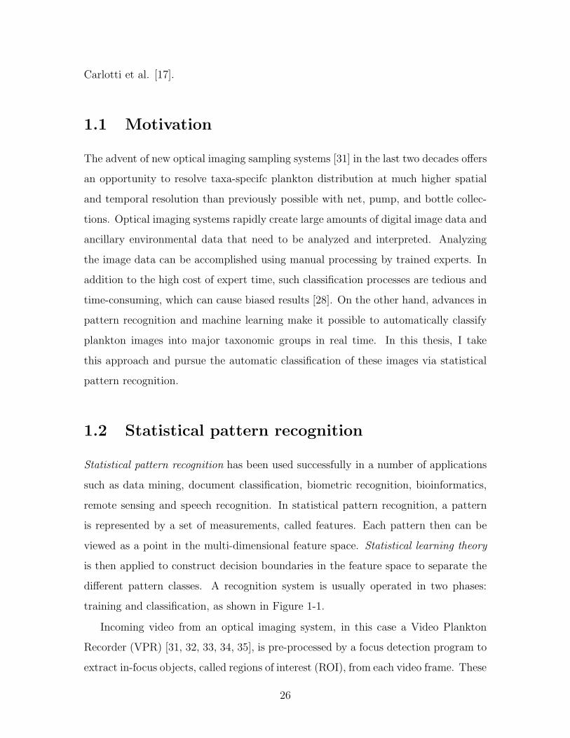
different pattern classes. A recognition system is usually operated in two phases:
training and classification, as shown in Figure 1-1.
Incoming video from an optical imaging system, in this case a Video Plankton
Recorder (VPR) [31, 32, 33, 34, 35], is pre-processed by a focus detection program to
extract in-focus objects, called regions of interest (ROI), from each video frame. These
26
ROIs are saved as Tagged Image File Format (TIFF) image files. A subset of these
files is manually labeled (identified), and serves as training samples. In the training
phase, a set of measurements (features) is computed from each image using different
pattern representation methods. Feature extraction is used to linearly combine dif-
ferent features and extract the most salient features for classification. Subsequently,
to train a classifier, a learning algorithm is employed to partition the feature space
into subspaces belonging to different classes (e.g., species). An important feedback
path allows a designer to interact with and optimize different pattern representation
methods, feature extraction algorithms and learning strategies. The arrows of pattern
representation and feature extraction between training and classification phases imply
that the same methods are used in classification which are optimized during training.
In the classification phase, the trained classifier uses the image-to-feature mapping,
which is learned during training, and assigns an input image to a class based on its
location relative to decision boundaries in the feature space.
1.2.1 Features
Features are measurable heuristic properties of patterns of interest. The rationale of
pattern representation and feature extraction is to avoid the curse of dimensionality
[8], the exponential growth of hypervolume as a function of dimensionality. For most
practical systems, labeled samples require expert time, thus are expensive to obtain,
that is to say, only limited labeled samples are available. In such cases, it has been
observed that additional features may degrade the classifier performance, which is re-
ferred to as the peaking phenomenon [76, 130, 129]. Thus a dimensionality reduction
(feature extraction and selection) step is essential, where only a small number of the
most salient features are selected to improve the generalization performance (classi-
fication performance on samples “unseen” during training) of a classification system.
At the same time, this step also reduces the storage requirements and processing
time.
27
Focus Detection
Pattern Representation
Feature Extraction
Classification
Incoming Video
ROIS
Feature Vector
Feature VectorClass Label
CLASSIFICATION PHASE
Classifier
Pattern Representation
Feature Extraction
Learning
Manually Sorting
Labelled ROIS
Feature Vector
Feature Vector
TRAINING PHASE
Figure 1-1: Schematic diagram of the pattern recognition system.
28

1.2.2 Statistical learning theory
The fundamental work of Vapnik [159, 160, 161] set the foundation for learning from
finite samples by using a functional analysis perspective with modern advances of
probability and statistics, and revived classical regularization theory. The basic idea
of Vapnik’s theory is to limit the model capacity by constraining decision boundaries
in a “small” hypothesis space, which is dependent on the training samples. This
is closely related to classical regularization theory in machine learning and overfit-
ting/overtraining in pattern recognition.
More formally, learning from examples can be formulated in the statistical learning
theory framework. Suppose we have two sets of variables x ∈ X ⊆ Rd and y ∈ Y ⊆ R.
A probability density function p(x, y) relates these two sets of variables over the whole
domain X × Y . We are provided with a data set Dl ≡ {(x, y) ∈ X × Y }l. They are
called the training data, and are obtained by sampling the probability density function
p(x, y) l times. Given the data set Dl, the problem of learning lies in providing an
estimator (a classifier/a learning machine) as a function fα : X → Y , which can be
used to predict a value of yi given any value of xi ∈ X. The functions fα(x) are
different mappings with adjustable parameters α. A standard way to solve the above
learning problem is to define a risk function, which computes the average amount of
error (cost) associated with an estimator, then choose the estimator which has the
lowest risk. The expected risk of an estimator is defined as,
R(fα) =
∫
x
∫
y
V (fα(x), y)p(x, y)dxdy. (1.1)
Here V is the loss function, and α are adjustable parameters. A particular choice of α
determines a learning machine. For example, a neural network with fixed architecture
is a learning machine, where α are the weights and bias of the network. The target
estimator is the function fα∗ which has minimal expected risk,
fα∗(x) = arg minα
R(fα) (1.2)
29
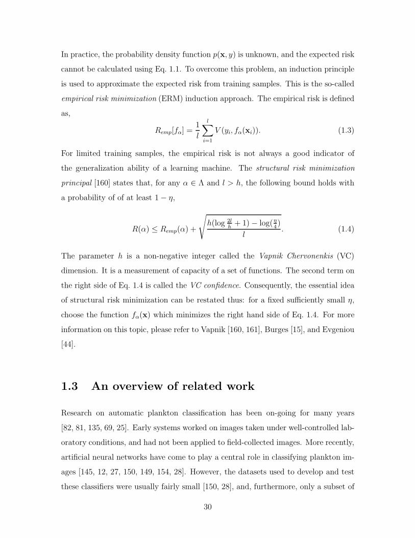
In practice, the probability density function p(x, y) is unknown, and the expected risk
cannot be calculated using Eq. 1.1. To overcome this problem, an induction principle
is used to approximate the expected risk from training samples. This is the so-called
empirical risk minimization (ERM) induction approach. The empirical risk is defined
as,
Remp[fα] =1
l
l∑
i=1
V (yi, fα(xi)). (1.3)
For limited training samples, the empirical risk is not always a good indicator of
the generalization ability of a learning machine. The structural risk minimization
principal [160] states that, for any α ∈ Λ and l > h, the following bound holds with
a probability of of at least 1 − η,
R(α) ≤ Remp(α) +
√
h(log 2lh
+ 1) − log(η4)
l. (1.4)
The parameter h is a non-negative integer called the Vapnik Chervonenkis (VC)
dimension. It is a measurement of capacity of a set of functions. The second term on
the right side of Eq. 1.4 is called the VC confidence. Consequently, the essential idea
of structural risk minimization can be restated thus: for a fixed sufficiently small η,
choose the function fα(x) which minimizes the right hand side of Eq. 1.4. For more
information on this topic, please refer to Vapnik [160, 161], Burges [15], and Evgeniou
[44].
1.3 An overview of related work
Research on automatic plankton classification has been on-going for many years
[82, 81, 135, 69, 25]. Early systems worked on images taken under well-controlled lab-
oratory conditions, and had not been applied to field-collected images. More recently,
artificial neural networks have come to play a central role in classifying plankton im-
ages [145, 12, 27, 150, 149, 154, 28]. However, the datasets used to develop and test
these classifiers were usually fairly small [150, 28], and, furthermore, only a subset of
30

distinctive images was chosen to both train and test the classifier. Since a classifier
needs to classify all the images from the field, including rare species and difficult ones,
even those that cannot be identified by a human expert, the accuracy reported for
a classifier built from only distinctive images will be generally optimistically biased.
The classifier performance was usually much worse when it was applied to all field
data [34].
The features used in the early systems were mostly shape-based. Jeffries et al. [81]
used moment invariants, Fourier descriptors and morphometric relations as features.
Although these features worked quite well under well-defined laboratory imaging con-
ditions and the overall recognition rate reported by Jeffries et al. was 90% for six
taxonomic groups, the system required significant human interaction and was not
suitable for in situ applications.
Initial automatic identification of VPR images was carried out using the method
described in Tang et al. [150] which introduced granulometry curves [162], along with
traditional features such as moment invariants, Fourier descriptors and morphome-
tric measurements. This method used a learning vector quantization (LVQ) neural
network as the classifier [149] and achieved 92% classification accuracy on a subset of
VPR images for six taxonomic groups. Only distinctive images were used in training
and testing the classifier in this initial study. A detailed experiment was conducted
in Chapter 3 to show the performance of the system when rare species and diffi-
cult images were included in training or testing samples. The average classification
performance on the whole dataset was 61% [34].
The performance disagreement between previous methods [81, 150] and current
study [34] is due to the nature of field-captured images. Unlike the well-controlled
laboratory conditions, field images are often occluded (objects truncated at edge of
image), and shape-based features such as moment invariants and Fourier descriptors
are very sensitive to occlusion. In addition, a significant number of field-collected im-
ages cannot be identified by a human expert due to object orientation and position in
the image volume1. These unidentifiable images were not used in training and testing
1Objects can be hard to identify due to their position in the image volume. If part of the object
31

the classifier [150] (although occluded images were included). A recent study by Luo
et al. [106] showed that including unidentifiable objects lowered the recognition rate
from 90% to 75% for their dataset from the shadow image particle profiling evaluation
recorder. In order to better estimate species specific abundance, a number of works
has shown that it was important to include an “other” [34] or “reject” [58] category.
In addition to occlusion, nonlinear illumination of images makes perfect segmenta-
tion (binarization) impossible, even after background brightness gradient correction.
Due to the grayscale gradient, the same object can have different segmented shapes
depending on where the object is in the field-of-view, thus causing shape-based fea-
tures to be less reliable.
Another type of feature we can extract from the grayscale images is a texture-based
feature. However, due to the early success of shape-based features on plankton images
from well-controlled laboratory imaging conditions, texture-based features have not
been widely used in plankton image recognition.
Texture-based features were compared against classic shape-based features. The
important finding was that the texture-based features were more important than the
shape-based features to classify field-collected plankton images. The main cause was
that texture-based features were less sensitive to occlusion and projection variance
than shape-based features.
1.4 Data
The data set was obtained from a 24-h VPR tow (VPR-7) in the Great South Chan-
nel off Cape Cod, Massachusetts, during June 1997 on the R/V Endeavor. The VPR
was towed from the ship in an undulating mode, forming a tow-yo pattern between
the surface to near bottom. The images were taken by the high magnification cam-
era, which had an image volume of 0.5ml. The total sampled volume during the
is out of this volume, the resulting image will be occluded. Nonlinear illumination makes objectsfrom the dark region more likely to be occluded by global segmentation, a problem correctable bybackground gradient removal [35]
32
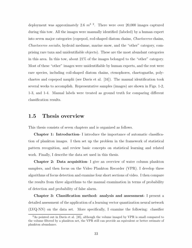
deployment was approximately 2.6 m3 2. There were over 20,000 images captured
during this tow. All the images were manually identified (labeled) by a human expert
into seven major categories (copepod, rod-shaped diatom chains, Chaetoceros chains,
Chaetoceros socialis, hydroid medusae, marine snow, and the “other” category, com-
prising rare taxa and unidentifiable objects). These are the most abundant categories
in this area. In this tow, about 21% of the images belonged to the “other” category.
Most of these “other” images were unidentifiable by human experts, and the rest were
rare species, including coil-shaped diatom chains, ctenophores, chaetognaths, poly-
chaetes and copepod nauplii (see Davis et al. [34]). The manual identification took
several weeks to accomplish. Representative samples (images) are shown in Figs. 1-2,
1-3, and 1-4. Manual labels were treated as ground truth for comparing different
classification results.
1.5 Thesis overview
This thesis consists of seven chapters and is organized as follows.
Chapter 1: Introduction- I introduce the importance of automatic classifica-
tion of plankton images. I then set up the problem in the framework of statistical
pattern recognition, and review basic concepts on statistical learning and related
work. Finally, I describe the data set used in this thesis.
Chapter 2: Data acquisition- I give an overview of water column plankton
samplers, and then focus on the Video Plankton Recorder (VPR). I develop three
algorithms of focus detection and examine four short sections of video. I then compare
the results from three algorithms to the manual examination in terms of probability
of detection and probability of false alarm.
Chapter 3: Classification method: analysis and assessment- I present a
detailed assessment of the application of a learning vector quantization neural network
(LVQ-NN) on the data set. More specifically, I examine the following: classifier
2As pointed out in Davis et al. [35], although the volume imaged by VPR is small compared tothe volume filtered by a plankton net, the VPR still can provide an equivalent or better estimate ofplankton abundance.
33

Figure 1-2: Example VPR images of copepods, rod-shaped diatom chain, Chaetoceros
socialis colonies and the “other” category. Fifty randomly selected samples are shown here.
34
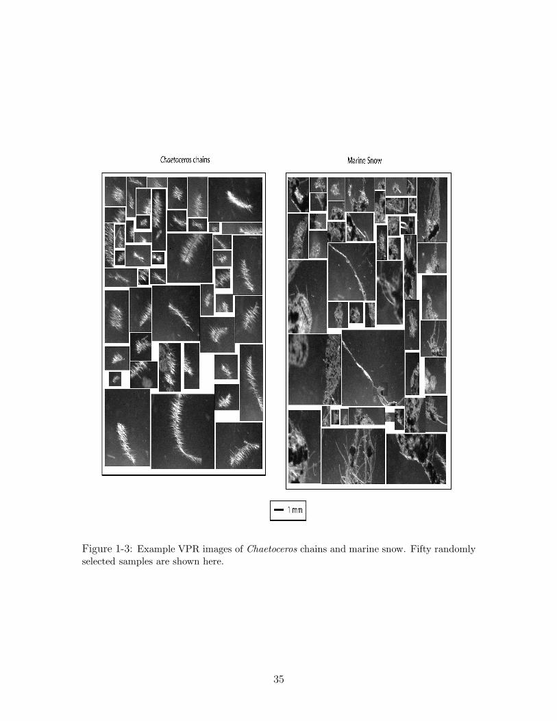
Figure 1-3: Example VPR images of Chaetoceros chains and marine snow. Fifty randomlyselected samples are shown here.
35
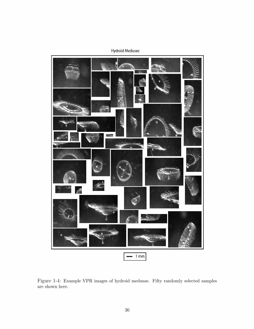
Figure 1-4: Example VPR images of hydroid medusae. Fifty randomly selected samplesare shown here.
36
complexity, feature length, learning curve, presentation order of training samples,
and different training samples. Next I propose a two-pass classification system and
compare the result with both the single LVQ-NN classifier and the single LVQ-NN
classifier with statistical correction. Finally, I modify the LVQ-NN to have an outlier
rejection metric based on the mean distance of correctly classified training samples.
Chapter 4: Pattern presentation- First I give an overview of pattern repre-
sentation/feature measurement methods. I group the pattern presentation methods
into three major groups, namely, shape-based, texture-based, and other methods. I
then conduct a comparison study between shape-based features and texture-based
features on a random set of the plankton data. I find the texture-based features
are more important than shape-based features to classify field-collected images. I
keep the comparison results as guidelines for choosing different feature presentation
methods in the later chapters.
Chapter 5: Co-occurrence matrices and support vector machine- I inves-
tigate the multi-scale co-occurrence matrices, and support vector machines to classify
the plankton image data set. From Chapter 4, I find that texture-based features are
more robust for classifying field-collected plankton images with occlusions, nonlin-
ear illumination and projection variance. I demonstrate that by using features from
multi-scale co-occurrence matrices and soft margin Gaussian kernel support vector
machine classifiers, a 72% overall probability of detection can be achieved compared
to that of 61% from a neural network classifier built on combinded shape-based fea-
tures. Subsequent plankton abundance estimates are improved in regions of low
relative abundance by more than 50%.
Chapter 6: Dual classification system- I incorporate a learning vector quan-
tization neural network classifier built from combined shape-based features and a
support vector machine classifier with texture-based features into a dual-classification
system. The system greatly reduces the false alarm rate of the classification, thus
extends the regions where the specificity curve of classification is relative flat, which
makes global correction of abundance estimation possible. After automatic correction,
the abundance estimation agrees very well both in high and low relative abundance
37

regions. For the first time, I demonstrate an automatic method which achieves abun-
dance estimation as accurately as human experts.
Chapter 7: Conclusions and future work- First, I summarize the major
contributions of this thesis, and then discuss the possibility of extending the existing
system to color or 3-D holographic images.
38

Chapter 2
Data Acquisition
In this chapter, I first overview water column plankton samplers in Section 2.1, then
decribe one specific optical sampler, the Video Plankton Recorder, in detail in Section
2.2. The main focus of this chapter is to discuss the focus detection program, which
is discussed in Section 2.3. I develop three new focus detection algorithms, and
compare them against human judgment on four video sections from VPR. This is the
first quantitative study of focus detection.
2.1 Water column plankton samplers
The development of quantitative zooplankton sampling systems can be traced back
to the late 19th and early 20th centuries. Non-opening/closing nets [67, 83], simple
opening/closing nets [71] and high-speed samplers [4] all began to be employed at
that time. All these systems have evolved with advances in technology, and are still
widely used for plankton survey programs. For example, non-opening/closing nets,
such as the Working Party 2 (WP2) net [49], modified Juday net [1], and Marine
Resources Monitoring Assessment Prediction (MARMAP) Bongo net [126] are still
used in large ocean surveys; simple opening/closing nets similar to those developed
by Hoyle [71], Leavitt [96], Clarke and Bumpus [24] are still manufactured and used;
high-speed samplers are also in use, such as the continuous plankton recorder [60],
which has evolved over 30 years, and become the main sampling system in the North
39

Atlantic plankton survey [164].
Since the 1950s, the concept of plankton patchiness has been well established,
and it triggered the development of closing cod-end systems and multiple net systems
in the 1950s and 1960s. Cod-end samplers such as the Longhurst-Hardy plankton
recorder [103] had problems with hang-ups and stalling of animals in the net which
caused smearing of the distributions of animals and loss of animals from the recorder
box [63]. The system was modified by Haury et al. to reduce these sources of bias
and used to study plankton patchiness in a variety of locations [62, 64]. Multiple net
systems [169, 172] were developed to fix these problems by opening and closing nets
in specific portions of the water column.
With the advances in charge-coupled device (CCD) and computer technology,
the 1980s and 1990s saw a boom of optical plankton sampling systems. Optical
systems have a number of advantages over net-based systems. The optical systems
can provide much finer vertical and horizontal spatial resolution than the net-based
systems. Optical systems have the potential to provide abundance estimates at short
temporal intervals along the tow path [32]. Furthermore, delicate and particulate
matter that may be damaged by net collection can be quantified by optical systems
[5, 38]. Image-forming systems have the potential to map taxa-specific distribution
in real time [34]. However, optical systems usually have a smaller sampling volume
than net-based systems given the same tow length. Thus rare organisms may remain
undetected with optical sampling systems.
Optical systems can be divided into two categories depending on whether the sys-
tem produces images of organisms or not. Non-image-forming systems such as the
optical plankton counter [68] use the interruption of a light source to detect and esti-
mate particle size. The family of image-forming systems has grown continuously since
1990. The Ichthyoplankton Recorder (IR) [50, 99], Video Plankton Recorder (VPR)
[31], Underwater Video Profiler (UVP) [55], Optical-Acoustic Submersible Imaging
System (OASIS) [75], In situ Video Camera [152], FlowCam [144], Holocamera [88],
Shadowed Image Particle Profiling and Evaluation Recorder (SIPPER) [138], Zoo-
plankton Visualization and Imaging System (ZOOVIS) [10], HOLOCAM [166], In
40
situ CritterCam [147], and Optical Serial Section Tomography (OSST) [48] all belong
to this category. In this thesis, images from the VPR were used. However, the algo-
rithms developed in this thesis are generic, and readily applied to images from other
optical plankton sampling systems.
Another group of plankton sampling systems is acoustic-based [170, 47]. Such
systems use acoustic backscattering to measure the size distribution of particles and
plankton. Hybrid systems also have been developed, combining optical and acous-
tic sampling, e.g., the VPR has been combined with multifrequency acoustics on
the BIo-Optical Multi-frequency Acoustical and Physical Environmental Recorder
(BIOMAPER-II) [173]. For more detailed review of plankton sampling systems,
please refer to Wiebe and Benfield [168].
Imaging plankton at sea while towing the sampler through the water at a 1-6 m/s,
requires a combination of magnifying optics, short exposure time, and long working
distance ( 0.5 m). The long working distance is needed to minimize detection and
avoidance of the sampler by the plankton. The short exposure time (e.g., 1 µs) is
obtained using a strobe. The density of pixels on the CCD array, together with the
need to image enough details of the individual plankton to identify them, limits the
camera’s field-of-view (FOV) to 1 cm for most mesozooplankton. For a depth of focus
of 3 cm, the image volume is 3 cm3, and video rate of 60 fields per second (FPS),
yields 0.18 liter of water imaged per second. Given a typical coastal concentration of
mesozooplankton of 10 individuals per liter, the time between individual sightings is
0.55 seconds, and at 60 FPS, there are 33 video fields between sightings. Thus, only
a small fraction of the video fields will contain mesozooplankton. For typical survey
periods of several hours or days, the volume of video data collected is much too large
for human operators to process manually. (For example, VPR has the bandwidth of
6 Mb/s or 518 Gb/day). Automatic pre-processing of the data is essential [31, 33].
In this chapter, I focus on one such pre-processing method called focus detection.
Before discussing this method, a detailed description of the VPR is necessary.
41

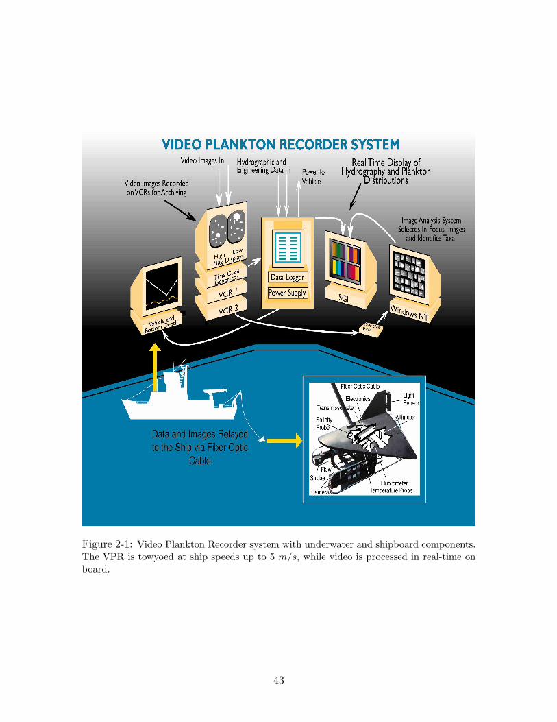
2.2 Video Plankton Recorder
The VPR system includes an underwater unit with video and environmental sensors,
and a deck unit for data logging, analysis and display (Figure 2-1). The underwater
unit has a video system with magnifying optics that images plankton and seston
in the size range of 100 microns to several centimeters [31, 33, 34, 35]. The initial
design [31] had four SONY XC-77 CCD cameras configured to simultaneously image
concentric volumes at different magnifications. The fields of view of the four cameras
were 0.7 × 0.56, 3 × 2.4, 5 × 4, and 8 × 6.4 cm2 respectively. Depths of field were
adjustable by different aperture settings. The sampled image volumes in each field
ranged from 0.5 ml to 1 liter depending on the optical settings. The modified system
[33, 34] had two analog video cameras of high and low magnification respectively.
The high magnification camera had an image volume of about 0.5 ml per field, while
the low magnification camera had an image volume of about 33 ml per field. Early
testing determined that these two cameras provided the most useful information. The
high-magnification camera provided detailed images permitting identification to the
species level, while the low-magnification camera imaged larger organisms such as
ctenophores and euphausiids. Positioning the image volume at the leading edge of
the tow-body and having a wide separation of the cameras and strobe, permitted
imaging of animals in their natural undisturbed state.
The images studied in this thesis came from the high magnification camera, which
had a pixel resolution of about 10 microns. The cameras were synchronized at 60 fields
per second to a xenon strobe1. The VPR also included a suite of auxiliary sensors
that measured pressure, temperature, salinity, fluorescence, beam attenuation, down-
welling light, pitch, roll, velocity and altitude. The environmental and flight control
sensors were sampled at 3 to 6 Hz. The underwater unit was towyoed at 4 ms−1
using a 1.73 cm diameter triple-armor electro-optical cable. Video and environmental
data from the towbody were received via a fiber optic cable into the data logging and
1The current system has a single 1008×1018 digital camera with field of view from 5×5 mm2 to20×20 mm2, and the depth-of-field is objectively calibrated using a tethered organism. The imageswere sampled at 30 frames per second [35]
42
��������������������������������������������������������������������������������������������������������������������������������������������������������������������������������������������������������������������������������������������������������������������������������������������������������������������������������������������������������������������������������������������������������������������������������������������������������������������������������������������������������������������
Figure 2-1: Video Plankton Recorder system with underwater and shipboard components.The VPR is towyoed at ship speeds up to 5 m/s, while video is processed in real-time onboard.
43

focus detection computer on the ship.
The deck unit consisted of a video recording/display system, an environmen-
tal/navigational data logging system, an image processing system and a data dis-
play system. Video was time-stamped at 60 fields per second and recorded on SVHS
recorders. The video time code was synchronized with the time from the P-code
Global Positioning System. Latitude and longitude were logged with video time code
and environmental data at 3 Hz on a personal computer and a Silicon Graphics Inc
(SGI) workstation.
2.3 Focus Detection
Video with time code from the high magnification camera was sent to the focus
detection system, which included an image processor interfaced to a computer. Video
was first digitized at field rates, then in-focus objects were detected using an edge
detection algorithm. The regions of interest (ROI) were saved to the hard disk as
tagged image format files using the video time code as the filename.
2.3.1 Objective
The main objective of the focus detection algorithm is data reduction. The video
comes in from the video camera at 60 fields per second. As discussed above, a large
proportion of fields are devoid of in-focus objects. Early systems required a human
operator to scan through all the video fields to determine when an in-focus organism
was observed and to what species it belonged. Such processes were very slow and
tedious, and introduced a source of subjective error when a line was drawn between
in-focus and out-of-focus objects. This line could vary from person to person, and
from time to time. The objective of the focus detection algorithm is to replace the
human operator with a program which objectively extracts in-focus objects from the
video images. The focus detection algorithm is required to extract as many in-focus
objects as possible, while picking up as few out-of-focus objects as possible, all in real
time. More formally, the focus detection program needs to have a high probability
44
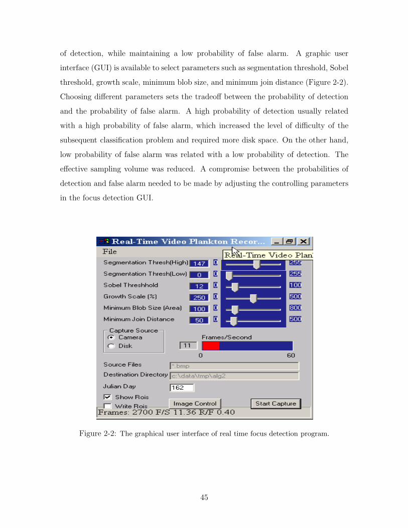
of detection, while maintaining a low probability of false alarm. A graphic user
interface (GUI) is available to select parameters such as segmentation threshold, Sobel
threshold, growth scale, minimum blob size, and minimum join distance (Figure 2-2).
Choosing different parameters sets the tradeoff between the probability of detection
and the probability of false alarm. A high probability of detection usually related
with a high probability of false alarm, which increased the level of difficulty of the
subsequent classification problem and required more disk space. On the other hand,
low probability of false alarm was related with a low probability of detection. The
effective sampling volume was reduced. A compromise between the probabilities of
detection and false alarm needed to be made by adjusting the controlling parameters
in the focus detection GUI.
Figure 2-2: The graphical user interface of real time focus detection program.
45

2.3.2 Method
In-focus object detection involves brightness correction, segmentation, labeling, size
thresholding, edge detection, edge thresholding, coalescing and ROI generation. In-
coming videos are dynamically adjusted to correct temporal changes in mean bright-
ness by shifting the mean brightness of each video frame to a certain value. Transla-
tion instead of scaling is used in this normalization step to avoid changing brightness
gradients within the frame. Brightness correction is followed by segmentation which
involves binarization of gray-scale images into binary images. Pixels with brightness
above the threshold value are set as foreground while the rest of the pixels are set as
background. After segmentation, a connectivity algorithm is used to check how the
foreground pixels connect to form blobs. The distinct blobs then are labeled from 1
to N , where N is the number of blobs present in the video field. Due to the imaging
environment, there are many small blobs present in each frame. Since small objects
are impossible to identify in the later processing and require much processing time, a
size threshold is imposed, and consequently blobs below a minimum number of pixels
are ignored. A rectangular bounding box is placed around each blob which passes
size thresholding. A Sobel operator is applied to each blob to calculate the brightness
gradient of the subimages. The small gradients in the subimages are considered to be
noise instead of real edges, and the gradients of each subimage are further thresholded
in order to suppress this noise.
Three in-focus algorithms are developed based on these thresholded gradients. If
the blob is in-focus, the center position and size are saved. After in-focus checking
on all the blobs from one field is completed, the bounding box of an in-focus blob is
extended/shrunk according to the GUI growth scale setting. Planktonic organisms
usually are partially transparent or translucent. When binarized, one organism often
breaks into several blobs. A coalesce operation is applied to group the close in-focus
blobs into one blob. Two or more blobs are considered to coalesce if there are overlaps
after the bounding boxes relax or if the central distance between them is below a user-
defined value on GUI. The resulting subimage inside the bounding box is called region
46
of interest (ROI), and is written to the disk as Tagged Image File Format with ROI
capture time as filename.
2.3.3 Algorithms
The motivation of the following algorithms is based on the observation that sharp
in-focus objects usually have strong edges (high gradient) between themselves and
their background, as well as inside themselves; while out-of-focus objects usually
lack such features. However, there are always exceptions. One such exception is
that highly saturated objects often reveal strong gradient between the objects and
their background whether the objects are in-focus or not. Such artifacts are due
to saturation of the objects. Three heuristic algorithms were developed to decide
whether an object was in-focus based on the gradient information.
1. Algorithm A1 (edge pixels only):
A1 is an algorithm which ignores the strength of the gradient after the pixel is
determined as edge pixel. The number of edge pixels is defined as the number
of pixels whose gradient values are greater than some user specified threshold.
The focus level index is defined as,
FL =Ne
A, (2.1)
where FL is the focus level index, Ne is the number of edge pixels, and A is the
area which is the number of foreground pixels in the subimage. The object is
considered in-focus if FL is greater than a fixed value.
2. Algorithm A2 (edge strength and additive brightness correction):
A2 is an algorithm which makes use of the number of edge pixels and their
gradient strength. In order to eliminate over-saturated blobs, which appear to
have a strong gradient at the boundary, a brightness compensation is made
to penalize such instances. The additive brightness correction is used in this
approach. The additive brightness correction is calculated as the difference
47
between the mean brightness in the subimage and the mean brightness of the
field. The focus level index is calculated as,
FL =A
4 × Ne
×Ne∑
i=1
Gi − Bc, (2.2)
Gi is the gradient values from the subimage above a certain threshold, A is
the area of subimage defined as in A1, Ne is the number of edge pixels whose
gradient values are above a certain threshold, and Bc is the additive brightness
correction term. An object is considered to be in-focus when FL is greater than
a user specified threshold.
3. Algorithm A3 (edge strength and multiplicative brightness correction):
A3 is an algorithm which uses only the gradient strength of edge pixels as well as
a multiplicative brightness correction. The multiplicative brightness correction
is calculated as the differences between the brightness in the subimage and the
mean brightness of the field. The focus level index was calculated as follows,
FL = c ×∑Ne
i=1 Gi∑Ns
j=1 Bc
, (2.3)
where FL is focus level index, c is a scaling constant, Ne is the number of edge
pixels defined as in A2, Gi is the gradient values from each subimage, and Ns
is the number of pixels in the subimage. Bc is the multiplicative brightness
correction term.
2.3.4 Result
Two video sections of the high magnification camera from cruise AN9703 in Mas-
sachusetts Bay conducted during March 11-15 1997 were manually examined and
used to “ground truth” the results of the three algorithms described above. The
videos were originally recorded on SVHS tape and later dubbed to BETACAM-SP
tape. The rationale of using BETACAM tape was to allow the human operator to go
48

through the videos field by field more easily. During the manual counting process, a
human operator examined each field with the assistance of the segmentation program.
The total number of all the objects (numbers of blobs in segmented image) as well as
the number of in-focus objects in each field were recorded. Extremely high concen-
trations of the colonial planktonic alga Phaeocystis were observed on the examined
tape. Only two seconds of video were examined, for each of two sections. Three focus
detection algorithms were tested on these two sections of video. The outputs of each
algorithm were further examined by the same human operator, and the number of
in-focus/out-of-focus images was counted. The results are summarized in Tables 2.1,
and 2.2.
Table 2.1: Comparison of focus detection algorithms from AN9703, high magnificationcamera, video section 1. The numbers are blob counts; probability of detection Pd
and probability of false alarm Pf are given as percentages.
Methods In-focus Out-of-focus Pd Pf
Manual count 132 808 NA NAA1 70 10 53% 1.2%A2 75 11 57% 1.4%A3 77 13 58% 1.6%
Table 2.2: Comparison of focus detection algorithms from AN9703, high magnificationcamera, video section 2. The numbers are blob counts; probability of detection Pd
and probability of false alarm Pf are given as percentages.
Methods In-focus Out-of-focus Pd Pf
Manual count 169 698 NA NAA1 82 8 49% 1.1%A2 89 15 46% 2.1%A3 87 11 51% 1.6%
The relative low probability of detection was due to the bottle-neck of the ROI
file-writing process, since there was an extremely high rate of ROI detection for
Phaeocystis. The whole process was synchronized in real time. Each field had only
16 milliseconds of processing time at most (since the video rate was 60 FPS). If it
took too long to process one field, the following fields would be skipped. In order
49

to take this bottleneck into account, the focus detection algorithms were run on a
paused field which had one in-focus object (but still output the video signal at 60
FPS). The number of files which were written out during a one-minute interval was
counted. The ratio between this number and the ideal number (3600 in this case) was
the correction factor due to the slow-down caused by the disk writing process. The
Pd after correction for video section 1 was quite good, because the average number of
in-focus objects present in this section was very close to 1 per field. However, for video
section 2, the average in-focus objects were close to 1.5 per field. Since a field cannot
have 1.5 in-focus objects, the same correction factor was used for both sections. Not
surprisingly, even after correction, Pd was still relatively low in video section 2. The
corrected results are shown in Tables 2.3, and 2.4. It is worth mentioning that this
problem would be vanished with a computer having a faster hard drive (the computer
used in the test was a 1 GHz Dell, circa 2000). Furthermore, such a dense patch of
Phaeocystis was not usual for the focus detection program. The average in-focus
object rate in most field applications was less than 1 per second compared to more
than 60 per second in this case.
Table 2.3: Comparison of focus detection algorithms from AN9703, high magnificationcamera, video section 1 after correction. The numbers are blob counts; probability ofdetection Pd and probability of false alarm Pf are given as percentages.
Methods In-focus Out-of-focus Pd Pf
Manual count 132 808 NA NAA1 111 16 84% 2.0%A2 120 18 91% 2.2%A3 123 21 93% 2.6%
Two video sections of the low-magnification camera from cruise HALOS, Cape
Cod Bay, March 1996, were also used to test the focus detection algorithms. Again,
the videos were dubbed from SVHS to BETACAM-SP. In this tape, very high con-
centrations of Pseudocalanus with eggs were observed. Five second intervals of video
were examined by a human operator since the concentration of the Pseudocalanus was
not as high as the Phaeocystis. The manual counting process and post-processing by
the focus-detection algorithm were the same as described above. The results are given
50

Table 2.4: Comparison of focus detection algorithms from AN9703, high magnificationcamera, video section 2 after correction. The numbers are blob counts; probability ofdetection Pd and probability of false alarm Pf are given as percentages.
Methods In-focus Out-of-focus Pd Pf
Manual count 169 698 NA NAA1 131 13 77% 1.9%A2 142 24 84% 3.4%A3 131 17 77% 2.4%
in Tables 2.5, and 2.6. The relative low value of Pd in Table 2.6 was due to a high
number of in-focus objects. The process of writing files affected the performance of
the algorithms, again correctable by a computer with faster hard disk drive.
Overall, all three algorithms did quite a good job on picking up in-focus objects,
while rejecting out-of-focus objects. The algorithms that took the gradient strength
into account (A2 and A3) worked a little better than the algorithm that thresholded
gradient information. Between the two strategies of brightness correction, the additive
worked as well as the multiplicative. Different parameter settings on the GUI (Fig 2-
2) trade-off between Pd and Pf . Since there were much higher numbers of out-of-focus
objects than in-focus objects on the video, the outcome of focus detection algorithm
was more sensitive to changes in Pf than Pd. Another way to look at this issue is
to check the percentage of in-focus objects from the outcome of each algorithm. For
example, in Table 2.6, of 132 images chosen by A3 to be in-focus, 107 images were
truly in-focus. That is to say, 81% of the output from A3 was true positive. A low true
positive rate will increase the difficulty level of the subsequent classification problem
and waste computational resources and disk space. On the other hand, a high true
positive rate may result in undersampling the underlying population of plankton.
The manual counting process only counted the number of in-focus objects and out-
of-focus objects on each field. For each algorithm, the output images were examined
by the same human operator in order to decide how many objects were in-focus
and out-of-focus. The whole process was subjective. For each object, the image
was not co-registered from the video to output images of each algorithm. The co-
registration of every single object would be labor intensive. However, by only counting
51

Table 2.5: Comparison of focus detection algorithms from HALOS, low magnificationcamera, video section 1. The numbers are the blob counts; probability of detectionPd and probability of false alarm Pf are given as percentages.
Methods In-focus Out-of-focus Pd Pf
Manual count 116 597 NA NAA1 89 23 77% 3.9%A2 98 16 84% 2.7%A3 107 25 92% 4.2%
Table 2.6: Comparison of focus detection algorithms from HALOS, low magnificationcamera, video section 2. The numbers are the blob counts; probability of detectionPd and probability of false alarm Pf are given as percentages.
Methods In focus Out focus Pd Pf
Manual count 161 736 NA NAA1 106 32 66% 4.4%A2 110 28 68% 3.8%A3 121 30 75% 4.1%
the number of in-focus and out-of-focus objects, additional error was introduced by
self-inconsistency. Nevertheless, this was the first quantitative study of focus detection
algorithms. A correction factor is needed to interpret the focus detection output in
the regions of extremely high plankton concentration.
2.4 Conclusion
A very large amount of data collected from an image-forming plankton sampler re-
quires an automatic focus detection program to extract only in-focus objects from
video. In this chapter, three algorithms were developed and tested on four video
sections from VPR. This was the first quantitative study of focus detection program
algorithms. In general, the algorithms have good performance for extracting in-focus
objects without extracting too many out-of-focus objects. However, care is needed
to interpret the focus detection output, especially in the regions of extremely high
plankton concentration.
52
Chapter 3
Classification Method: Analysis
and Assessment
A learning vector quantization neural network (LVQ-NN) classification system with
combined shape-based features has been investigated. The objective of this study
was to fully understand how the LVQ-NN classification system behaved on the field-
collected plankton data. Multiple factors such as classifier complexity, number of
training samples, quality of training samples, feature length, and presentation order
of training samples have been examined. Three different methods have been proposed
and implemented to improve the LVQ-NN classifier. This study suggested that the
LVQ-NN classification system was very robust to varied parameter changes. However,
for shape-based features, there was very limited improvement on classifying field-
collected plankton images. The big classification performance difference between this
study and previous studies indicated that previously reported accuracy of LVQ-NN
was optimistically biased. Part of the results in this chapter was published in Marine
Ecology Progress Series[34].
This chapter is organized as follows. In Section 3.1, I describe a state-of-the-art
LVQ-NN classification system developed by Tang [150]. This system is well accepted
but not well assessed. In Section 3.2, I investigate this system by changing classi-
fier complexity, feature length, numbers of training samples, initial neuron position,
presentation order of training samples, different training samples and classification
53

stability. In Section 3.3, I develop a two-pass classification system based on this
LVQ-NN classification system. In Section 3.4, I propose a method to correct the
bias of the classification system. In Section 3.5, I develop a distance rejection metric
on LVQ-NN classification system. Part of the results discussed in this chapter was
published in Davis et al.[34]
3.1 System overview
3.1.1 Artificial Neural Networks
Artificial Neural Networks (ANN) have experienced three periods of extensive activ-
ity. The first peak in the 1940s was due to McCulloch’s pioneering work [113]. The
second in the 1960s was Rosenblatt’s perceptron convergence theorem [136]. Minsky
[116] showed that a single perceptron was not able to solve a simple XOR problem.
Such limitation dampened the progress in ANN. The third peak was due to the Hop-
field’s energy approach [70] and back-propagation learning algorithm for multilayer
perceptrons by Werbos [167], and later popularized by Rumelhart [137].
The great benefits of the ANN are the simplicity of the learning algorithm, the
ease in model selection, and incorporation of heuristic information and constraints.
ANN has been widely used in feature extraction [110, 105], character classification
[97, 98], speaker identification [124], and general object classification [148, 150].
3.1.2 Learning vector quantization neural network classifier
Learning vector quantization (LVQ) is a supervised version of vector quantization. Its
objective is to learn a set of prototypes (codebooks) which best represent each class.
We implement it with an artificial neural network [150, 34]. The neural network has
two layers, namely a competitive layer and a linear output layer. The complexity
of the neural network (prototypes of subclass, number of neurons) is based on the
number of training samples and the number of classes in the classifier. The number
of output layer neurons is equal to the number of taxa. The weights of the neurons
54
for each class are initialized to be the mean of the training feature vectors for that
class plus a small random value. The network is trained by randomly presenting the
training samples to the network. Each training sample is classified by the current
LVQ neural network. Depending on the outcome of the classifier, the weights of the
neurons are adjusted in the following two ways: If the predicted label of a sample
agrees with its true label, the weights of the winning neuron (prototype) are updated
in such a way that the winning neuron moves a step closer to the training sample in
the feature space; otherwise, the weights of the winning neuron are updated such that
the winning neuron is pushed a step away from the training sample in the feature
space. The training process stops when the preset goal or the maximum training time
is reached. The trained network is saved as the final classifier.
3.1.3 Principal component analysis
Principal Component Analysis (PCA) is widely used in signal processing, statistics,
and pattern recognition [84]. Denote x = (x1, x2, · · · , xn)T as a n-dimensional original
feature vector, and y = (y1, y2, · · · , ym)T as a m-dimensional final feature vector
(m ≤ n), PCA seeks a linear transformation T, such that
y = Tx, (3.1)
where T is m × n matrix. The main idea of the transformation is to explain the
maximum amount of variance in n-dimensional vector x by a much lower dimensional
vector y. In other words, PCA seeks a linear projection that best represents the data
in the mean-square sense.
In order to find the transformation matrix T, p observations of x (p training
samples, p ≥ n) are required. First, the n-dimensional mean vector µ and n × n
covariance matrix Σ are computed from all the training samples. Next, the eigenvec-
tors and eigenvalues are computed from the covariance matrix, and sorted according
to decreasing order of eigenvalue. Denoting these eigenvectors as e1, e2, · · · , en and
corresponding eigenvalues as λ1, λ2, · · · , λn, and choosing the m eigenvectors having
55

the largest eigenvalues, we form an m × n matrix T whose rows are transposes of
the m eigenvectors. The representation of data by PCA projects the data onto the
m-dimensional subspace according to
y = T(x − µ). (3.2)
3.1.4 Feature extraction
For each sample image, four different groups of feature presentation methods are used,
which include 7 moment invariants, 64 Fourier descriptors, 160 pattern spectra, and 6
morphological measurements. These features are combined into a single feature vector
with 237 elements. All the feature elements are first normalized to zero mean and
unit standard deviation. Principal component analysis is then applied on this feature
vector to eliminate linear dependence among elements of the feature vector. The 20-30
largest eigenvalues account for nearly all the variances in feature space of the training
samples. The corresponding eigenvectors are saved and used as a transformation
matrix. All the non-training samples are normalized and projected onto these 20-30
orthogonal bases via the transformation matrix. The resulting feature vector is the
input of the LVQ neural network classifier.
3.1.5 Classification performance estimation
After a classifier has been built, its classification generalization performance (perfor-
mance from a set of independent samples) needs to be evaluated. For finite sample
sizes and unknown class-conditional distribution, the only way to estimate the gen-
eralization performance is to use an empirical method. There are three empirical
ways to estimate the generalization performance. The first approach is often called
the resubstitution method, which involves classifying all the training samples, and
uses classification accuracy on training samples as generalization performance. It is
fast and does not require extra labeled samples. Nevertheless, this method has an
optimistically biased estimate of classification performance.
56

The second approach is often called the cross-validation method, which can be
further divided into three cases. The first case is often called holdout method, which
uses a completely independent test data set to evaluate generalization performance
of a classifier. The drawback of this method is that it requires twice as many labeled
samples as resubstitution. According to Jain et al. [77], this estimate is pessimistically
biased. From the results in this chapter, I do not get any pessimistically biased
estimates. I used the holdout method as a classification performance estimate from
the whole data set. Since there is an overlap between training samples and test
samples, strictly speaking, it is a misnomer. However, the overlap is small and the
difference between training accuracy and test accuracy of the classifier is also small.
I argue that the difference between the “true” holdout and my pseudo-holdout is
negligible.
The second case of the cross-validation method is often called the leave-one-out
method, which involves building n classifiers with n− 1 training samples. Each time,
a different sample is left out to build a classifier and used to test the classifier. Here
n is the number of total training samples. The leave-one-out method is computation
demanding, and it has an unbiased estimate with large variance [77]. The third case
of the cross-validation method is the rotation method, also called an n-fold cross
validation method, which is a compromise between the holdout and leave-one-out
methods. It divides the training samples into p disjoint subsets, using p − 1 subsets
for training a classifier and the remaining subset for testing the classifier.
The third approach is called the bootstrap method, which involves generating
multiple bootstrap sample sets of size n by sampling all the training samples with
replacement. The bootstrap bias and variance estimate can be estimated from boot-
strap sample sets. When the number of bootstraps approaches infinity, the boot-
strap variance becomes the traditional variance of mean [42]. In this chapter, the
resubstitution, leave-one-out, and holdout methods are used to estimate classification
performance.
57

3.2 Assessment Result
3.2.1 Classifier complexity vs. classifier performance
The relationship between classifier performance and classifier complexity is investi-
gated first. The classifier complexity is characterized by the number of neurons per
taxon, which governs the expressive power of the neural network. The neurons are
evenly distributed among taxa. Classifiers with 3 neurons per taxon up to 100 neu-
rons per taxon are trained with the same amount of training samples. The training
samples come from a mixture of four VPR tows from the same cruise [34]. Each
classifier is applied to all the images from a single VPR tow, which includes more
than 20,000 images. Classification accuracy is obtained by comparing the predicted
classification label with the human label for each image. The classification accuracy
rises from 3 to 4 neurons per taxon, reaches its peak at 10 to 15 neurons per taxon,
and then hovers around with an overall accuracy of 59-60% (Figure 3-1). No obvious
over-training effect is observed. This can be seen more clearly in Figure 3-2. How-
ever, when a large number of neurons is used, the classifier takes a long time to train.
Furthermore, when classification performance is inferred from training accuracy (e.g.
resubstitution method), using a large number of neurons can result in a large bias on
the classification accuracy estimation (for example, Tang [148, 150] used an average
of training and test accuracy to compare classification performance).
3.2.2 Feature length versus classification performance
Final feature length may play an important role in classification performance. Choos-
ing a short feature length may lose the discriminative power of the feature set, while
choosing a long feature length may include noise to degrade classification performance.
In this study, feature lengths from 2 to 40 are examined. Again, classifiers are trained
from a mixture of four VPR tows from the same cruise. A total of 70 neurons are
used to train the classifiers, which are evenly divided into 7 taxa with 10 neurons
per taxa. The classification performance of different taxa varies differently with the
58

3 4 6 10 15 20 30 50 1000
50
100Copepod
3 4 6 10 15 20 30 50 1000
50
100Rod−shaped diatom chains
3 4 6 10 15 20 30 50 1000
50
100 Chaetoceros chains
Cla
ssifi
catio
n ac
cura
cy (%
)
3 4 6 10 15 20 30 50 1000
50
100 Chaetoceros socialis chains
3 4 6 10 15 20 30 50 1000
50
100Hydroid medusae
Numbers of neurons per taxon 3 4 6 10 15 20 30 50 100
0
50
100Marine snow
Numbers of neurons per taxon
Figure 3-1: Classification performance with respect to classifier complexity.
0 10 20 30 40 50 60 70 80 90 10040
50
60
70
80
90
100
Numbers of neurons per taxon
Cla
ssific
atio
n a
ccu
racy
test accuracytraining accuracy
Figure 3-2: Training and test accuracy with respect to classifier complexity.
59

change of feature length (Figure 3-3). Some taxa have relatively steady classification
performance, while the others have more variations with the change of feature length.
However, the overall classification performance (average over all the taxa) is fairly
steady and reveals a slight increase with increasing feature length (Figure 3-4). The
steady increase of training accuracy with feature length suggests that extra features
capture training sample specific features instead of general features of each taxon.
On the other hand, the test accuracy curve is fairly flat from the feature lengths from
20 to 40 (Figure 3-4).
2 5 10 15 20 25 30 35 400
50
100Copepod
2 5 10 15 20 25 30 35 400
50
100Rod−shaped diatom chains
2 5 10 15 20 25 30 35 400
50
100 Chaetoceros chains
Clas
sifica
tion
accu
racy
(%)
2 5 10 15 20 25 30 35 400
50
100 Chaetoceros socialis chains
2 5 10 15 20 25 30 35 400
50
100Hydroid medusae
Feature length 2 5 10 15 20 25 30 35 40
0
50
100Marine snow
Feature length
Figure 3-3: Classification performance as a function of feature length for each taxon.
3.2.3 Learning curve - numbers of training samples versus
classifier performance
The number of training samples is an important factor for supervised learning. Few
training samples may not fully present the feature space, while a large number of
60

0 5 10 15 20 25 30 35 4030
40
50
60
70
80
90
100
Feature length
Cla
ssific
atio
n a
ccu
racy
test accuracytraining accuracy
Figure 3-4: Training and test accuracy with respect to feature length.
training samples are very costly to get because labeling requires extensive expert
time. Training on a very large data set is also computationally intensive, which may
take days or even months. In this study, the relationship between the number of
training samples and classification performance is explored empirically. The objec-
tive is to understand how many training samples are “good” enough in the sense of
manual labeling efficiency. Training samples are randomly selected from the whole
data set. The classification performance as a function of training sample size for each
taxon is shown in Figure 3-5. In general, classification performance tends to increase
with more training samples being available. For copepod and rod-shaped diatom
chains, classification accuracy remains almost the same from 50 samples per taxon to
400 samples per taxon. For other taxa, classification accuracy increases with more
training samples added. Compared to Figure 3-1 and Figure 3-5, there are signifi-
cant differences of classification accuracy for copepod and rod-shaped diatom chains.
Such differences are caused by different training samples used. I will discuss more on
the training samples effect later in this chapter. Figure 3-6 shows training and test
classification accuracy with respect to training sample size (learning curve). From 50
to 200 training samples per taxon, the test classification accuracy has an increase of
61

4% with respect to an increase of 100 samples per taxon. From 200 training samples
to 400 training samples per taxon, the increase of test classification accuracy drops
down to 0.5% with an increase of 100 samples per taxon. I conclude that 200 train-
ing samples per taxon is the optimal number of training samples in terms of manual
labeling efficiency. Hereafter, 200 training samples per taxon are used if it is not
explicitly stated. However, as shown in Figure 3-5, the optimum training samples
per taxon is taxon dependent. For relatively “easy” taxon such as rod-shaped diatom
chains, a small number of training samples are sufficient. On the other hand, for really
“hard” taxon such as copepods, considering large within-taxonomic group variation
of copepods, such difference in training sample size has small effect on classifcation
accuracy.
50 100 200 4000
50
100Copepod
50 100 200 4000
50
100Rod−shaped diatom chains
50 100 200 4000
50
100 Chaetoceros chains
Cla
ssifi
catio
n ac
cura
cy (%
)
50 100 200 4000
50
100 Chaetoceros socialis chains
50 100 200 4000
50
100Hydroid medusae
Training samples 50 100 200 400
0
50
100Marine snow
Training samples
Figure 3-5: Classification performance as a function of training sample size for eachtaxon.
62

0 50 100 150 200 250 300 350 40040
50
60
70
80
90
100
Training sample size
Cla
ssific
atio
n a
ccu
racy
test accuracytraining accuracy
Figure 3-6: Training and test accuracy with respect to training sample size.
3.2.4 Initial neuron position versus presentation order of train-
ing samples
There are two sources of randomness when the classifiers have been trained with the
same training samples. The first one is the initial positions of neurons before the train-
ing processes start. The second one is the presentation orders of the training samples
to the classifiers. Both randomized initial position of neurons and presentation order
of training samples are used in order to speed up the learning process. In this section,
I investigate which source of randomness may have the largest impact on classification
performance. Two sets of tests are conducted. In both sets of tests, each classifier
is built on the same training samples with 200 training samples per taxon randomly
selected from the whole data set. For simplicity, the resubstitution method is used
to evaluate classification accuracy. Since the classification performance is compared
in the relative sense, I have used training accuracy as a classification performance
indicator. The mean and standard deviation of training accuracy are calculated from
10 different trials. The difference between the first set of tests and the second set of
tests is that in the first set of tests each classifier has both different initial position of
63

neurons and different presentation order of training samples, while in the second set
of tests each classifier starts with same initial position of neurons and is trained with
different presentation order of training samples. The result is shown in Figure 3-7.
The mean and standard deviation of the classification performance are almost identi-
cal, which suggests that different initial positions of neurons have little effect on the
final classifiers. This agrees a well known result that the random presentation order
of training samples has more impact on classification performance.
IP1 IP20
20
40
60
80
100Copepod
IP1 IP20
20
40
60
80
100Rod−shaped diatom chains
IP1 IP20
20
40
60
80
100 Chaetoceros chains
IP1 IP20
20
40
60
80
100 Chaetoceros socialis chains
Clas
sifica
tion a
ccura
cy (%
)
IP1 IP20
20
40
60
80
100Hydroid medusae
IP1 IP20
20
40
60
80
100Marine snow
Figure 3-7: Comparison between the random initial position of neurons and randomorder of presentation order of training samples. IP1 - different initial position ofneurons, random representation order of training samples; IP2 - same initial positionof neurons, random representation order of training samples
3.2.5 Training samples effect
Classifiers are not only affected by the size of the training samples, but also by the
quality of the training samples. We have already seen from Figure 3-1 and Figure 3-5
that different training samples significantly affect the classification accuracy of cope-
pod and rod-shaped diatom chains. In this section, we try to quantify classification
performance variations from different training samples. Three sets of tests have been
64
conducted for this manner. For all the tests, training samples are randomly selected
from the whole data set with 200 samples per taxon. In the first set of tests (TS1),
each classifier is built from different training samples, and is then evaluated by the
leave-one-out method. In the second set of tests (TS2), each classifier is also built
from different training samples, and is evaluated by the holdout method. In the third
set of tests (TS3), each classifier is built from the same training samples, and eval-
uated by the holdout method. The results are shown in Figure 3-8. It is interesting
to see that the leave-one-out method has high estimates on certain taxa such as rod-
shaped diatom chain and hydroid medusae, while it has low estimates on other taxa
such as copepod and Chaetoceros chains. This does not agree with the statement that
the leave-one-out estimate is unbiased and the holdout estimate is pessimistically bi-
ased by Jain et al. [77]. The overall classification accuracy is very close between
the leave-one-out method and the holdout method, given that training samples are
randomly selected from the whole data set. Otherwise, the cross validation (leave-
one-out) method may still have a biased estimate of classification accuracy [34]. In
general, the variation of classification accuracy (variance of mean accuracy) is much
smaller when classifers are trained by a single set of training samples than different
sets of training samples. Such variation is also taxon dependent. For “easy” taxon
such as rod-shaped diatom chains, the variation is much smaller compared to “hard”
taxon such as copepods. The variation of the leave-one-out method is similar to that
of the holdout method.
3.2.6 Classification stability
The stability of a classfier, namely, how the classifier is affected by changing the
training samples, has been used to study generalization performance of the classfier
by many researchers theoretically [13, 43]. In this section, I have investigated stability
of our LVQ-NN classifier in terms of variance of abundance estimation of each taxon.
Nine classifiers are built from different random sets of training samples, which contain
200 samples for each taxon, and are randomly picked from the whole data set. Each
classifier is then used to classify the whole data set. The mean and standard deviation
65

TS1 TS2 TS30
20
40
60
80
100Copepod
TS1 TS2 TS30
20
40
60
80
100Rod−shaped diatom chains
TS1 TS2 TS30
20
40
60
80
100 Chaetoceros chains
TS1 TS2 TS30
20
40
60
80
100 Chaetoceros socialis chains
Clas
sifica
tion a
ccura
cy (%
)
TS1 TS2 TS30
20
40
60
80
100Hydroid medusae
TS1 TS2 TS30
20
40
60
80
100Marine snow
Figure 3-8: Comparison of different training samples effect on classfication perfor-mance. TS1 - different sets of training samples, leave-one-out method; TS2 - differentsets of training samples, holdout method; TS3 - single set training samples, holdoutmethod
abundance are calculated. The mean, upper and lower limit of 95% confidence in-
terval abundances are ploted against manually sorted abundance (Figure 3-9). Most
taxa have stable classification results except copepods, which show a large difference
between the upper and lower limit of 95% confidence interval.
3.3 Two-pass classification system
When a classifier is used to estimate abundance, there are two sources which make
the estimation biased. The first source is the relative abundance of each taxon. The
classifier tends to underestimate the relative high abundance taxon and overestimate
the relative low abundance taxon. For example, suppose that a sample contains 2
taxa, with 90 individuals of one taxon and 10 individuals of the other taxon. For both
taxa, the classifier has the probability of detection of 90%. The expected number of
individuals classified as the first taxon is (90×0.9)+(10×0.1) = 82 and the expected
number classified as the second taxon is (10 × 0.9) + (90 × 0.1) = 18. Despite the
66

5 10 15 20 250
1
2
3
4Copepods
5 10 15 20 250
1
2
3
4Rod−shaped diatom chains
5 10 15 20 250
1
2
3
4 Chaetoceros chains
Abs
olut
e a
bund
ance
(#
indi
vidu
als
/ lite
r)
5 10 15 20 250
1
2
3
4 Chaetoceros socialis colonies
Abs
olut
e a
bund
ance
(#
indi
vidu
als
/ lite
r)
5 10 15 20 250
1
2
3
4Hydroid medusae
Hour of Day(GMT)5 10 15 20 25
0
1
2
3
4Marine snow
Hour of Day(GMT)
manually sortedclassification meanup 95% confidence intervallow 95% confidence interval
Figure 3-9: Mean, upper and lower limit of 95% confidence interval of abundanceestimates from LVQ-NN classifiers and that of manually sorted results. Time seriesabundance plots along the tow path are shown for 6 dominant taxa. Data were firstbinned in 10 second time intervals, and a one-hour smoothing window was applied tothe binned data.
67

classifier having a relative high probability of detection of 90%, the abundance of the
rare taxon in the sample is, on average, overestimated by a factor of nearly 2. The
second source is uneven probability of detection. It is easy to show in the two taxa
case. Suppose that a sample contains 2 taxa, with 50 individuals of one taxon and
50 individuals of the other taxon. The classifier has probabilities of detection of 90%
and 50% for each taxon, respectively. The expected number of individuals classified
as the first taxon is (50 × 0.9) + (50 × 0.5) = 70 and the expected number classified
as the second taxon is (50 × 0.5) + (50 × 0.1) = 30. Although two taxa are equally
abundant, the classifier has overestimated the taxon with the higher probability of
detection.
3.3.1 Decision rules
The above problem arises from uneven distribution and probability of detection. One
way to overcome such a problem is to design a classifier under minimax criterion.
Briefly speaking, one first searches for the prior for which the Bayes risk is maximum,
one then finds the decision boundary to minimize the above Bayes risk. The solution
is often called the minimax solution. Denoting that R1 is the region in feature space
where the classifier decides ω1, and likewise R2 decides ω2, one can write the overall
risk of the classifier in terms of conditional risks [42]:
R =
∫
R1
[λ11P (ω1)p(x|ω1) + λ12P (ω2)p(x|ω2)]dx
+
∫
R2
[λ21P (ω1)p(x|ω1) + λ22P (ω2)p(x|ω2)]dx, (3.3)
where P (ωi) is prior probability, p(x|ωi) is conditional probability, and λij is the loss
function. If one uses the fact that P (ω1) = 1 − P (ω2) and that∫
R1
p(x|ω1)dx =
68
1 −∫
R2
p(x|ω2)]dx, one can rewrite the above risk function as:
R(P (ω1)) = λ22 + (λ12 − λ22)
∫
R1
p(x|ω2)]dx
+ P (ω1)[(λ11 − λ22) + (λ21 − λ11)
∫
R2
p(x|ω1)dx − (λ12 − λ22)
∫
R1
p(x|ω2)]dx].
(3.4)
If one sets the second term at the right hand side of the above equation equal to
zero, the risk function is independent of prior probabilities. Such a solution is called
a minimax solution. When the zero-one loss function is used, i.e.,
λij =
{
0 i = j
1 i 6= j,(3.5)
the condition of the minimax solution can be simplified as,
∫
R2
p(x|ω1)dx −∫
R1
p(x|ω2)]dx = 0. (3.6)
Another way is to use recursive prior estimation. Since in most real world problems,
the form of the conditional probability distribution is complicated or even unknown,
finding the decision boundary of the minimax solution is not trivial. In this section,
we adopt the second approach, that is to say, we try to recursively estimate the priors.
The three most popular decision rules are illustrated in Figure 3-10. The max-
imum likelihood (ML) decision rule seeks the intersection between two conditional
probability distributions, and the corresponding decision value is x∗ML. The max-
imum a posteriori (MAP) decision rule seeks the intersection between two scaled
conditional probability distributions, and the corresponding decision value is x∗MAP .
The scaling factor is the ratio of the priors of the two classes. The minimax decision
rule seeks a decision value x∗MM which makes the areas under the two distribution
tails equal.
In my application, I have used classification to estimate the fine resolution of
priors for each taxon. Before classification, nothing is known about the priors, so a
69

−5 50
0.1
0.2
0.3
0.4
0.5
0.6
p(x | ω1)
p(x | ω2)
P(ω1)/P(ω
2)*p(x | ω
1)
x*ML
x*MAPx*
MM
p(x | ω1)
p(x | ω2)
P(ω1)/P(ω
2)*p(x | ω
1)
Figure 3-10: Illustration of the three most popular decision rules. x∗ML - maximum
likelihood decision rule, x∗MAP - maximum a posteriori decision rule, x∗
MM - minimaxdecision rule
ML decision rule is applied in the first classifier. Local priors can be estimated from
the first classification results using a moving window average method (for example,
calculate from the latest 100 samples). The priors estimated from the first classifier
are then applied in the second classifier based on a MAP decision rule. I call such a
system a two-pass classifier since each sample needs to be classified twice.
The structure of the two-pass classifier is shown in Figure 3-11. There are two
classifiers involved in the two-pass classification system. The first classifier is the same
as a single classifier, the outcomes of which are used to estimate local priors for each
taxon. The predictions of the first classifier are collected by a prior estimator. After
collecting a certain number of samples, local priors of each taxon will be reported by
the prior estimator. These local priors are updated afterwards when a new sample
is available. The second classifier utilizes the local priors as well as the same feature
vector used in the first classifier to get a better prediction for each sample. For
simplicity, the algorithms of the two classifiers are identical, the only difference is the
priors of each taxon. Priors of the first classifier are set to uniform for all taxa, while
priors of the second classifier are calculated from the prior estimator. The rationale
70

of two-pass classification is that as long as the first classifier is better than a random
guess, the priors estimated from it are much better than uniform priors. Given this
piece of information, the second classifier will further improve the prediction of each
sample beyond that of the first classifier.
3.3.2 Implementation
To summarize the above discussion, the two-pass classification system can be imple-
mented in the following steps:
1. Train a LVQ neural network classifier with an equal number of training samples
for each taxon.
2. Generate a confusion matrix with the leave-one-out method from training sam-
ples. Calculate the probability of detection (Pd) for each taxon.
3. For each field sample, classify it with the classifier built above.
4. Set up a first-in-first-out (FIFO) queue. If the queue is not filled, output the
predicted class label, and go to step 2. Otherwise update priors for each taxon.
5. Use the probability of detection to correct the priors.
6. Calculate the scaling factors C(ωi) =√
(1 − P (ωi)) for each taxon based on
their priors.
7. Use the second classifier to compute the distance map between the sample and
neurons, scale the distance map with scaling factor C(ωi).
8. Make the prediction based on the modified distance map and go back to step 2.
3.3.3 Results
Abundance estimations of six dominant taxa are compared among manually sorted,
single NN classifier and two-pass NN classifier with combined features of moment in-
variants, Fourier descriptors, pattern spectra and morphological measurements (Fig-
71

Focus Detection
Pattern Representation
Feature Extraction
Classification 1
Incoming Video
ROIS
Feature Vector
Feature Vector
CLASSIFICATION PHASE
Classifier
Pattern Representation
Feature Extraction
Learning
Manually Sorting
Labelled ROIS
Feature Vector
Feature Vector
TRAINING PHASE
Prior Estimation
Classification 2
Class Label
Class Label
Priors
Figure 3-11: Schematic diagram of two pass classification system
72
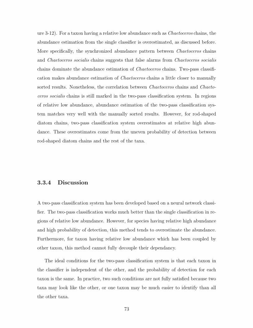
ure 3-12). For a taxon having a relative low abundance such as Chaetoceros chains, the
abundance estimation from the single classifier is overestimated, as discussed before.
More specifically, the synchronized abundance pattern between Chaetoceros chains
and Chaetoceros socialis chains suggests that false alarms from Chaetoceros socialis
chains dominate the abundance estimation of Chaetoceros chains. Two-pass classifi-
cation makes abundance estimation of Chaetoceros chains a little closer to manually
sorted results. Nonetheless, the correlation between Chaetoceros chains and Chaeto-
ceros socialis chains is still marked in the two-pass classification system. In regions
of relative low abundance, abundance estimation of the two-pass classification sys-
tem matches very well with the manually sorted results. However, for rod-shaped
diatom chains, two-pass classification system overestimates at relative high abun-
dance. These overestimates come from the uneven probability of detection between
rod-shaped diatom chains and the rest of the taxa.
3.3.4 Discussion
A two-pass classification system has been developed based on a neural network classi-
fier. The two-pass classification works much better than the single classification in re-
gions of relative low abundance. However, for species having relative high abundance
and high probability of detection, this method tends to overestimate the abundance.
Furthermore, for taxon having relative low abundance which has been coupled by
other taxon, this method cannot fully decouple their dependancy.
The ideal conditions for the two-pass classification system is that each taxon in
the classifier is independent of the other, and the probability of detection for each
taxon is the same. In practice, two such conditions are not fully satisfied because two
taxa may look like the other, or one taxon may be much easier to identify than all
the other taxa.
73
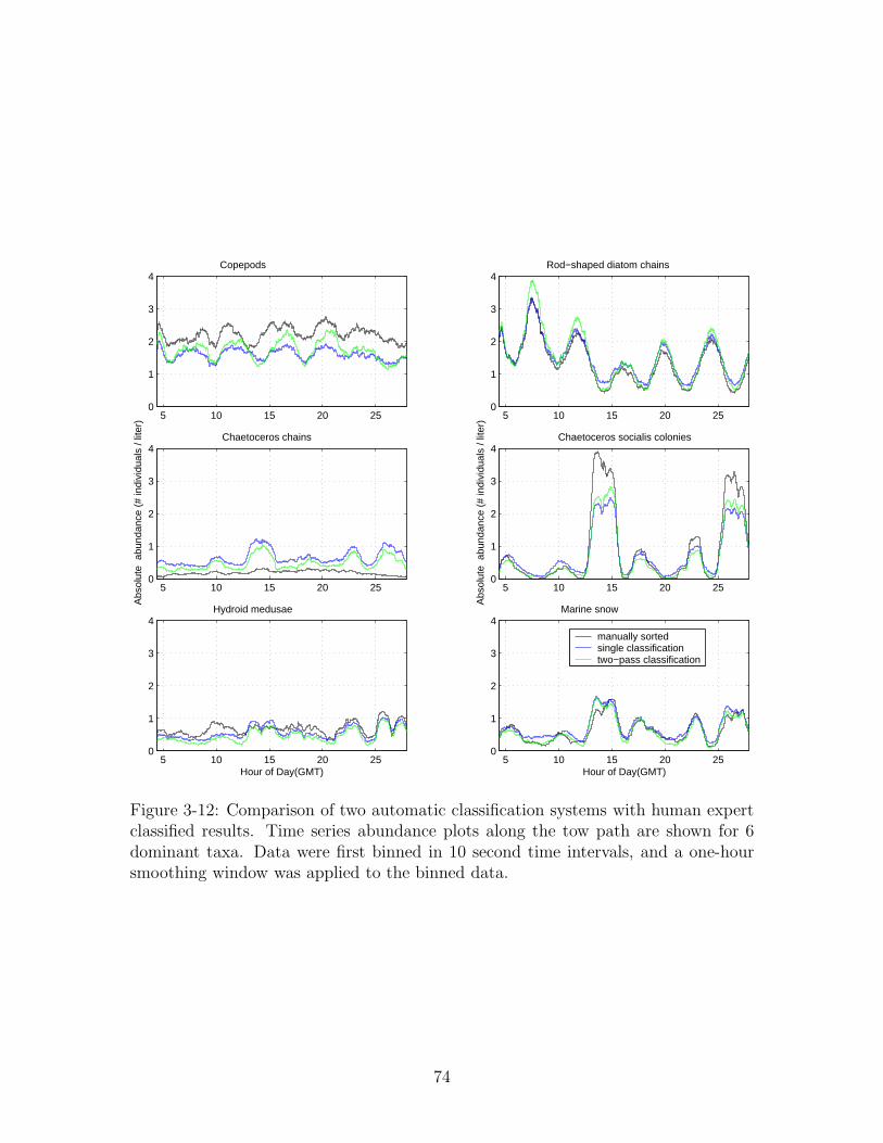
5 10 15 20 250
1
2
3
4Copepods
5 10 15 20 250
1
2
3
4Rod−shaped diatom chains
5 10 15 20 250
1
2
3
4 Chaetoceros chains
Abs
olut
e a
bund
ance
(#
indi
vidu
als
/ lite
r)
5 10 15 20 250
1
2
3
4 Chaetoceros socialis colonies
Abs
olut
e a
bund
ance
(#
indi
vidu
als
/ lite
r)
5 10 15 20 250
1
2
3
4Hydroid medusae
Hour of Day(GMT)5 10 15 20 25
0
1
2
3
4Marine snow
Hour of Day(GMT)
manually sortedsingle classificationtwo−pass classification
Figure 3-12: Comparison of two automatic classification systems with human expertclassified results. Time series abundance plots along the tow path are shown for 6dominant taxa. Data were first binned in 10 second time intervals, and a one-hoursmoothing window was applied to the binned data.
74
3.4 Statistical correction method
In the section, I try to correct bias from a single NN classification with a statistical
correction method (SCM). As discussed in the last section, when the relative abun-
dance is uneven and the classification system is not perfect, there is a high bias on
taxon abundance estimation which has low relative abundance. In this section, I
have proposed a method to correct this problem. Such a method is proposed by two
independent research groups [146, 174].
3.4.1 Method
Before I start, I need to define confusion matrix. A confusion matrix is a way to
quantify a classification system. It is an n×n matrix where n is the number of taxon
in the classifier. Elements mij are the probabilities that a randomly selected sample
of taxon ωj will be classified to taxon ωi by the classification system. Denote such a
matrix as M .
Suppose the classification process can be characterized in the following mathe-
matical model,
xC = MxT, (3.7)
where xC and xT are classified and true population proportion vectors. Assume M
is invertible, we can solve for xT using
xT = M−1xC. (3.8)
Now suppose an estimate of confusion matrix M can be obtained by applying the
classifier to a set of representative samples for each taxon or by the cross-validation
method on training samples. Replacing M by its estimated values M gives,
xT = M−1xC. (3.9)
xT is a maximum likelihood estimate of xT, given the characteristics of the classifi-
75

cation system described by the confusion matrix.
Negative abundance estimation may result from the above procedure, which indi-
cates that there is an error in estimation of the confusion matrix M . However, such
occurrences are very rare, given a fair wider smoothing window applied to the abun-
dance estimation. One can choose an easy way to fix the negative abundance problem
by setting negative abundance to zero and redistributing the net loss of abundance
to the rest of the taxa in the classifier.
3.4.2 Result
Abundance estimations of six dominant taxa are compared among manually sorted,
NN classifier and SCM with combined features of moment invariants, Fourier descrip-
tors, pattern spectra and morphological measurements (Figure 3-13). Apparently,
abundance estimation from SCM has lower bias compared to that of the automatic
classification method. On the other hand, abundance estimation from SCM also
yields a higher variance compared to that of the automatic classification method.
This phenomenon is well-known, and is called the bias-variance dilemma or bias-
variance trade-off, which states that classifiers with increased flexibility to adapt to
the training data tend to have lower bias but higher variance. SCM obviously has
much more flexibility than the uncorrected NN classifier.
Abundance estimation of rod-shaped diatom chains from SCM agrees very well
with manually sorted estimation, although the abundance estimation from the NN
classifier is already fairly good. On the other hand, abundance estimation of cope-
pods from SCM has much larger error than that of the NN classifier. For Chaetoceros
chains, SCM reduces the bias of abundance estimation; however, the artificial patch-
iness pattern still remains.
SCM yields lower bias and higher variance abundance estimation than the NN
classifier. For applications investigating large scale abundance patterns or low fre-
quency signals, SCM is a good method to use because some of the variance will go
away with a wider smoothing window. On the other hand, for applications inves-
tigating small scale abundance patterns or high frequency signals, SCM should be
76
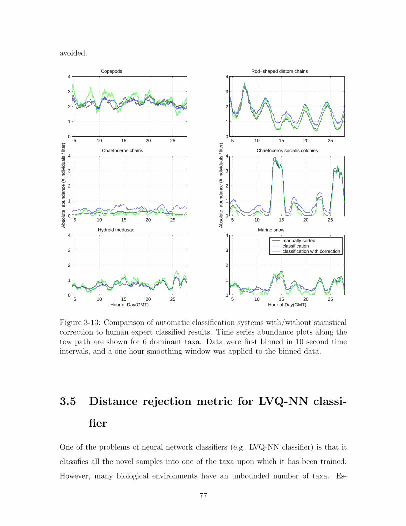
avoided.
5 10 15 20 250
1
2
3
4Copepods
5 10 15 20 250
1
2
3
4Rod−shaped diatom chains
5 10 15 20 250
1
2
3
4 Chaetoceros chains
Abs
olut
e a
bund
ance
(#
indi
vidu
als
/ lite
r)
5 10 15 20 250
1
2
3
4 Chaetoceros socialis colonies
Abs
olut
e a
bund
ance
(#
indi
vidu
als
/ lite
r)
5 10 15 20 250
1
2
3
4Hydroid medusae
Hour of Day(GMT)5 10 15 20 25
0
1
2
3
4Marine snow
Hour of Day(GMT)
manually sortedclassificationclassification with correction
Figure 3-13: Comparison of automatic classification systems with/without statisticalcorrection to human expert classified results. Time series abundance plots along thetow path are shown for 6 dominant taxa. Data were first binned in 10 second timeintervals, and a one-hour smoothing window was applied to the binned data.
3.5 Distance rejection metric for LVQ-NN classi-
fier
One of the problems of neural network classifiers (e.g. LVQ-NN classifier) is that it
classifies all the novel samples into one of the taxa upon which it has been trained.
However, many biological environments have an unbounded number of taxa. Es-
77

pecially for exploration cruises, the taxa encountered during the cruise are hard to
predict. Furthermore, in order for an LVQ-NN classifier to reliably recognize new
samples in each taxon, a certain number of samples in each taxon is required. In
many applications, there are not enough training samples to train an LVQ-NN clas-
sifier for some taxa. In such cases, it is essential for a classifier to be able to reject
the novel samples as “unknown” instead of classifying incorrectly into one of the taxa
in which the classifier has been trained. In this section, I have developed a rejection
metric based on distance map between neurons and test samples.
3.5.1 Distance rejection system
The schematic diagram is shown in Figure 3-14. The difference between an LVQ-
NN classification system with and without distance rejection metric is that, after a
normal LVQ-NN classifier has been trained, all the training samples are classified
once again by the freshly trained classifier; the distances between each sample and
the nearest neuron are recorded for every sample which is correctly classified by the
LVQ-NN classifier. Mean and standard deviation of the distances are calculated for
each class in the classifier and a distance outlier threshold has been computed from
the mean and standard deviation of the distance. That is to say, after training,
besides a normal LVQ-NN classifier, a set of distance outlier thresholds have been
obtained for each class in the classifier. During the classification process, when each
sample is classified by a normal LVQ-NN classifier, the distance between the sample
and the nearest neuron has been compared against the distance threshold of the class
upon which the normal LVQ-NN classifier is going to predict. If the distance is below
the threshold, the classifier predicts the label of the sample that is the same as that
neuron. Otherwise, the classifier predicts the label of the sample as “unknown”.
3.5.2 Result and discussion
In order to test the distance rejection metric, a random set of samples with 200 per
taxon for training and another 200 per taxon were drawn from the whole data set. In
78

PatternRepresentation
LVQ-NNLearning
Correct?
Yes
No
Calculate mean(m_i) and standard deviation(s_i)of the distance
for each class
Calculate distance outlier threshold dr_i = m_i + 2*s_i
Training
d < dr_i
Label the sample as same the class index as the neuron
Label the sampleas ’unknown’
Classification
Yes
No
FeatureExtraction
PatternRepresentation
FeatureExtraction
LVQ-NNClassification
Find the distance from the sample to the nearest neuron
Go to NextSample
Training Samples
PatternRepresentation
All Samples
FeatureExtraction
LVQ-NNClassification
Calculate the distance (d)
from the sample to the nearest
neuron
dr_i
d
Figure 3-14: Schematic diagram of distance rejection classification system
79
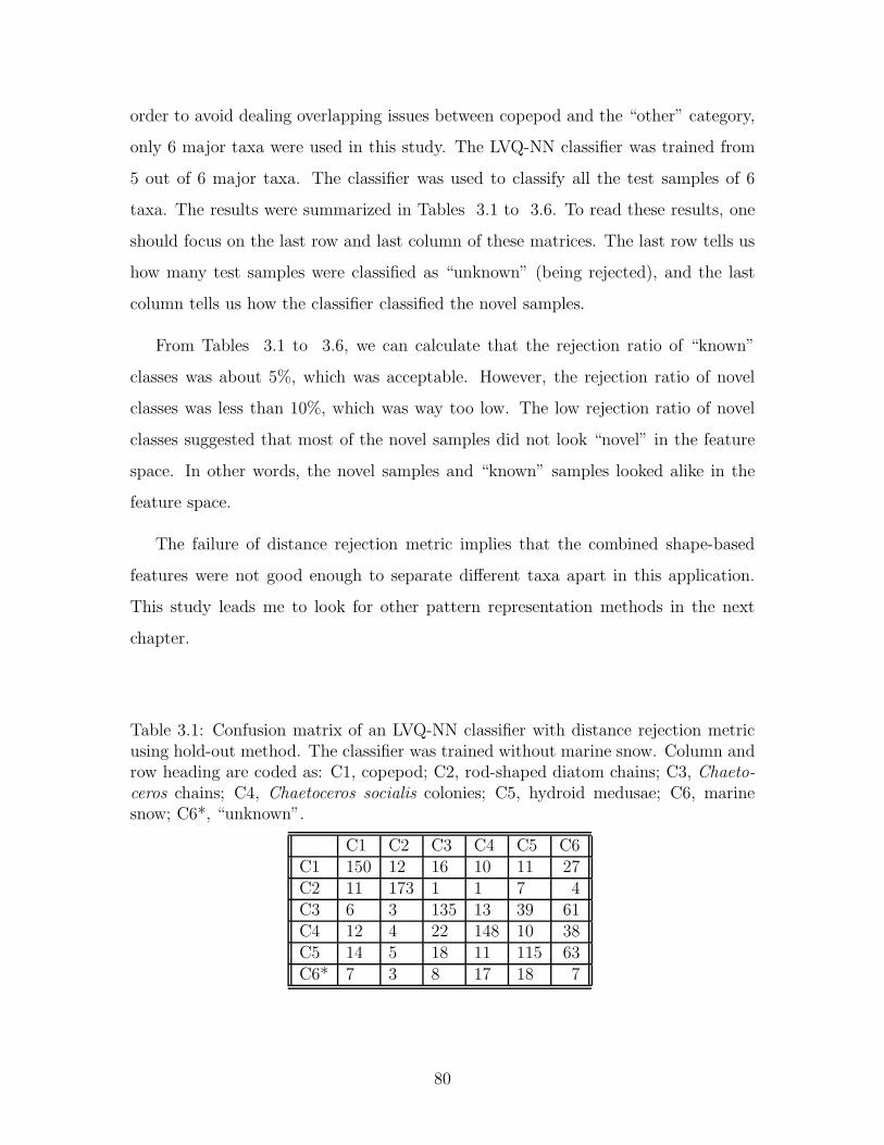
order to avoid dealing overlapping issues between copepod and the “other” category,
only 6 major taxa were used in this study. The LVQ-NN classifier was trained from
5 out of 6 major taxa. The classifier was used to classify all the test samples of 6
taxa. The results were summarized in Tables 3.1 to 3.6. To read these results, one
should focus on the last row and last column of these matrices. The last row tells us
how many test samples were classified as “unknown” (being rejected), and the last
column tells us how the classifier classified the novel samples.
From Tables 3.1 to 3.6, we can calculate that the rejection ratio of “known”
classes was about 5%, which was acceptable. However, the rejection ratio of novel
classes was less than 10%, which was way too low. The low rejection ratio of novel
classes suggested that most of the novel samples did not look “novel” in the feature
space. In other words, the novel samples and “known” samples looked alike in the
feature space.
The failure of distance rejection metric implies that the combined shape-based
features were not good enough to separate different taxa apart in this application.
This study leads me to look for other pattern representation methods in the next
chapter.
Table 3.1: Confusion matrix of an LVQ-NN classifier with distance rejection metricusing hold-out method. The classifier was trained without marine snow. Column androw heading are coded as: C1, copepod; C2, rod-shaped diatom chains; C3, Chaeto-ceros chains; C4, Chaetoceros socialis colonies; C5, hydroid medusae; C6, marinesnow; C6*, “unknown”.
C1 C2 C3 C4 C5 C6C1 150 12 16 10 11 27C2 11 173 1 1 7 4C3 6 3 135 13 39 61C4 12 4 22 148 10 38C5 14 5 18 11 115 63C6* 7 3 8 17 18 7
80

Table 3.2: Confusion matrix of an LVQ-NN classifier with distance rejection metricusing hold-out method. The classifier was trained without hydroid medusae. Columnand row heading are coded as: C1, copepod; C2, rod-shaped diatom chains; C3,Chaetoceros chains; C4, Chaetoceros socialis colonies; C5, marine snow; C6, hydroidmedusae; C6*, “unknown”.
C1 C2 C3 C4 C5 C6C1 133 14 11 6 13 11C2 18 166 4 6 0 11C3 7 3 131 18 32 40C4 11 2 12 136 21 16C5 18 7 30 23 125 92C6* 13 8 12 11 9 30
Table 3.3: Confusion matrix of an LVQ-NN classifier with distance rejection met-ric using hold-out method. The classifier was trained without Chaetoceros socialoscolonies. Column and row heading are coded as: C1, copepod; C2, rod-shaped di-atom chains; C3, Chaetoceros chains; C4, hydroid medusae; C5, marine snow; C6,Chaetoceros socialis colonies; C6*, “unknown”.
C1 C2 C3 C4 C5 C6C1 139 11 15 8 13 9C2 13 172 5 8 5 6C3 10 2 118 20 38 68C4 9 5 23 122 35 18C5 19 3 26 24 106 85C6* 10 7 13 18 3 14
Table 3.4: Confusion matrix of an LVQ-NN classifier with distance rejection metricusing hold-out method. The classifier was trained without Chaetoceros chains. Col-umn and row heading are coded as: C1, copepod; C2, rod-shaped diatom chains; C3,Chaetoceros socialos colonies; C4, hydroid medusae; C5, marine snow; C6, Chaeto-ceros chains; C6*, “unknown”.
C1 C2 C3 C4 C5 C6C1 144 10 3 5 17 25C2 5 169 3 5 5 0C3 10 2 153 14 42 28C4 9 2 9 122 37 57C5 20 8 24 39 94 73C6* 12 9 8 15 5 17
81

Table 3.5: Confusion matrix of an LVQ-NN classifier with distance rejection metricusing hold-out method. The classifier was trained without rod-shaped diatom chains.Column and row heading are coded as: C1, copepod; C2, Chaetoceros chains; C3,Chaetoceros socialis colonies; C4, hydroid medusae; C5, marine snow; C6, rod-shapeddiatom chains; C6*, “unknown”.
C1 C2 C3 C4 C5 C6C1 149 11 4 16 12 120C2 14 118 10 20 23 10C3 9 9 145 4 27 7C4 3 23 8 113 38 43C5 16 27 23 30 96 8C6* 9 12 10 17 4 12
Table 3.6: Confusion matrix of an LVQ-NN classifier with distance rejection metricusing hold-out method. The classifier was trained without copepod. Column and rowheading are coded as: C1, rod-shaped diatom chains; C2, Chaetoceros chains; C3,Chaetoceros socialis colonies; C4, hydroid medusae; C5, marine snow; C6, copepod;C6*, “unknown”.
C1 C2 C3 C4 C5 C6C1 176 4 3 2 5 45C2 6 118 17 25 25 55C3 2 16 136 5 32 20C4 4 17 12 122 35 18C5 8 33 23 27 99 38C6* 4 12 9 19 4 24
82

3.6 Conclusion
In this chapter, a classic learning vector quantization neural network classifier with
combined shape-based features was assessed. Multiple factors such as classifier com-
plexity, number of training samples, quality of training samples, feature length, classi-
fier stability, and presentation order of training samples were investigated. This study
showed that previous reported accuracy was optimistically biased. A two-pass classi-
fication system and a statistical correction method were developed on this classifier.
A distance rejection metric was also developed on the LVQ-NN classifier. The limited
improvement on various methods based on the LVQ-NN classifier suggested that the
shape-based features were not good enough to classify field-collected plankton images.
The study leads me to look for texture-based features in the next chapter.
83

84
Chapter 4
Pattern Representation/Feature
Measurement
This chapter covers the various pattern representation methods used to obtain fea-
tures from pattern images. Although pattern recognition has been well studied, pat-
tern does not have a well-accepted definition. According to Watanabe [165], a pattern
is opposite to a chaos; it is an entity, vaguely defined, that could be given a name.
For example, a pattern could be a human face image or an acoustic signal. In this
thesis, I consider a pattern as a view-based 2-D image of a 3-D object. In pattern
recognition/classification, a set of measurements which describes a pattern is of spe-
cial interest. These measurements are called features, and the step that calculates
features from pattern is called pattern representation or feature measurement1. Three
important cues to recognize an image object are shape, texture, and color. Similarly,
pattern representation methods can be grouped into shape-based, texture-based, and
color-based method. In this chapter, shape-based and texture-based feature methods
are discussed and compared using a random subset of the data set described in Chap-
ter 1. The images are in-focus regions-of-interest (ROIs) extracted from the full 2-D
grayscale images digitized from the VPR’s analog video (see Chapter 2).
This chapter is organized as follows. In Section 4.1, I review the pattern represen-
1A number of authors use the term feature extraction to cover all the processes from raw datato final feature set, which includes pattern representation and feature selection/extraction in ourterminology.
85

tation in the literature, and group them into 3 major categories, namely shape-based,
texture-based, and other methods. In Section 4.2, a selected representative methods
from each group and their feature extraction and classification method are described.
In Section 4.3, I compare selected pattern representation methods and different fea-
ture extraction for each method.
4.1 Pattern representation methods
4.1.1 Shape-based methods
Shape-based features are features calculated primarily from the shape of objects.
Classic examples of shape-based features are moment invariants and Fourier descip-
tors.
Moment Invariants
Moment invariants were first introduced by Hu [72] to classify planar objects. They
are one of the most extensively studied invariant features [7, 101, 131]. These orthog-
onal moment invariants are invariant to rotation, scale and translation (RST). For
non-negative integers p, q, the (p + q)th order moments of a pattern f(x, y) are given
as,
mp,q =
∫ ∞
−∞
∫ ∞
−∞
xpyqf(x, y)dxdy. (4.1)
Its discrete form is
mp,q =M
∑
x=1
N∑
y=1
f(x, y)xpyq, (4.2)
where the image is size of M ×N . The translation-invariant central moments of order
(p + q) are obtained by placing the origin at the center of gravity
µp,q =M
∑
x=1
N∑
y=1
f(x, y)(x− x)p(y − y)q, (4.3)
86

where x = m10/m00, y = m01/m00.
Hu showed that
νpq =µpq
µ(1+(p+q)/2), p + q ≥ 2 (4.4)
were scale-invariant, where µ = µ00 = m00. From combination of νpq’s, Hu [72]
derived seven moment invariants which were RST invariant.
Zernike moments
The Zernike polynomials were first introduced in 1934 [176]. For a set of complex
Zernike polynomials Vnm(x, y), which form a complete orthogonal basis defined within
the unit circle, Zernike moments of an image function f(x, y) are the projection of
the function onto Zernike polynomials
Anm =n + 1
π
∫ ∫
x2+y2≤1
f(x, y)[Vnm(x, y)]∗dxdy. (4.5)
Here n ≥ 0, |m| ≤ n, n − |m| is even, and the symbol ∗ denotes the complex
conjugate operator. A set of complex orthogonal polynomials Vnm(x, y) are defined
as
Vnm(x, y) = Rnm(x, y)ejmarctan(y/x), (4.6)
where j =√−1, n ≥ 0, |m| ≤ n, n − |m| is even, and
Rmn(x, y) =
(n−|m|)/2∑
s=0
(−1)s(x2 + y2)(n/2)−s(n − s)!
s!( (n+|m|)2
− s)!( (n−|m|)2
− s)!. (4.7)
For a digital image, the Zernike moment of order n and repetition m is given by
Anm =n + 1
π
∑ ∑
x2+y2≤1
f(x, y)[Vnm(x, y)]∗. (4.8)
Here the symbol ∗ denotes the complex conjugate operator.
Zernike polynomials are orthogonal and rotation invariant. Zernike moments have
nice properties in terms of noise sensitivity, information redundancy and reconstruc-
87

tion capability [151]. The amplitudes of the Zernike moments were used as features
for character recognition [7, 90, 91], texture classification [163], and invariant image
watermark [93].
Fourier-Mellin Transform
Let f(r, θ) be an intensity function of a two-dimensional image expressed in the polar
coordinates. By first applying the circular Fourier transform and then applying Mellin
transform to this function, we have the following transform as a function of l and w
z(l, w) =1
2π
∫ ∞
0
∫ 2π
0
f(r, θ)e−ilθriw−1dθdr. (4.9)
This is the so called Circular-Fourier Radial-Mellin Transform, or simply the Fourier-
Mellin Transform. The modulus of z(l, w) is invariant under both rotation and scaling.
The coefficients z(l, w) are often referred to as Fourier-Mellin descriptors. Their
magnitudes are often used as invariant features under the two-dimensional rotation
and scaling [36, 86, 141, 142, 143]. In order to achieve translation invariance, one can
shift the origin of polar coordinates at the center of gravity. Casasent and Psaltis
[18, 19] took the following alternative approach.
1. Calculate the power spectrum of the Fourier transform of the two-dimensional
input.
2. Convert the power spectrum to polar coordinates.
3. Perform a polar-log mapping.
4. Calculate another two-dimensional Fourier transform power spectrum.
The final power spectrum is RST invariant. Li [101] has identified that the normal-
ized Fourier-Mellin descriptors are linear combinations of some normalized geometric
moments.
88
Fourier Descriptors
Fourier descriptors (FD) are well studied invariant features used to describe a contour
of an object. Depending on what functions are used to describe a contour, FDs can
be grouped into 3 major categories, namely tangent-angle FDs proposed by Zahn
and Roskies [175], complex FDs first used by Granlund [57], and elliptic FDs by
Kuhl and Giardina [94]. FDs are the Fourier coefficients when the contour function is
approximated by Fourier series. More research effort has been devoted to the shape
classification by FDs [123, 102, 89]. For the most common used contour complex
function, each point on the contour can be represented by its complex coordinates,
z(l) = x(l) + jy(l). As a point moves along the contour in the counterclockwise
direction, it generates a complex function z(l). Suppose we normalize the perimeter
of the contour to 2π, then the function z(l) is periodic with the period of 2π. Such a
function can be approximated by a Fourier series,
z(l) =
∞∑
k=−∞
ckejkl. (4.10)
The coefficients can be calculated from the following integral,
ck =1
2π
∫ π
−π
z(l)e−jkldl. (4.11)
The normalized amplitude spectrum {|cn|/|c1|} (n 6= 0) is invariant to RST and
reflection.
Curvature and Shape Spectrum
Gaussian curvature (curvature for short) is an intrinsic property of a 2-dimensional
surface. It is independent of the coordinate system. In two dimensions, the extrinsic
curvature is defined as
κ ≡ dφ
ds, (4.12)
89

which can be calculated as
κ =x′y′′ − y′x′′
(x′2 + y′2)3/2(4.13)
The Gaussian curvature and mean curvature are defined from the two principal cur-
vatures. The Gaussian curvature is defined as the product of the two principal cur-
vatures, while mean curvature is the mean of the two principal curvatures. Gaussian
curvature is used as a shape descriptor to describe 3-D objects [132, 54]. Dorai and
Jain [41, 40] proposed to use the shape index to describe 3-D free-form objects. The
shape index is defined as
SI(p) =1
2− 1
πtan−1 κ1(p) + κ2(p)
κ1(p) − κ2(p), (4.14)
where κ1 and κ2 are the principal curvatures of the surface. The histogram of the
shape index is called the shape spectrum. Nastar[119] applied the shape spectrum to
real-time face recognition.
4.1.2 Texture-based methods
Image texture is a function of spatial variations in pixel intensities. It is difficult
to give texture a formal definition [156]. On the other hand, texture is the most
important visual cue in identifying different types of homogeneous images via their
texture properties. Most natural surfaces reveal unique texture. Texture analysis has
applications in texture classification, segmentation and synthesis.
Autocorrelation and Power Spectrum
In a simple model, texture is considered as a repetitive placement of texture elements
(primitive or texton) in the image. The autocorrelation method [127] is based on find-
ing linear spatial relationships between primitives. Given a gray-scale image f(x, y),
the autocorrelation function is defined as
Cp,q =
∑Mx=1
∑Ny=1 f(x, y)f(x + p, y + q)
∑Mx=1
∑Ny=1 f 2(x, y)
. (4.15)
90
If the primitives are large, the function decreases slowly with increasing distance,
whereas it decreases rapidly if texture consists of small primitives. The power spec-
trum is highly related to autocorrelation function. The discrete Fourier transform of
an image f(n1, n2) is defined by
F (k1, k2) =
N1−1∑
n1=0
N2−1∑
n2=0
f(n1, n2)e−j(2π/N1)k1n1e−j(2π/N2)k2n2,
0 ≤ k1 ≤ N1 − 1, 0 ≤ k2 ≤ N2 − 1,
0, otherwise.
(4.16)
The power spectrum is defined as
P (k1, k2) = F (k1, k2) · F (k1, k2)∗. (4.17)
Co-occurrence Matrices
Spatial gray level co-occurrence matrices estimate second-order statistics from the
images. Julesz [85] did pioneering work on texture analysis with first-order and
second-order statistics. The co-occurrence matrices method was first proposed by
Haralick [59] as a texture feature and it has been widely used thereafter. It is based
on estimation of the joint probability distribution of pixels with gray level i and j,
a spatial distance d, and angle θ in an image. If the texture is coarse and distance
d is small compared to the size of texture primitive, the pairs of points should have
similar gray levels. Conversely, for a fine texture, if distance d is comparable to the
texture size, the gray levels of point pairs should be quite different. The value in
the co-occurrence matrix should be spread out relatively uniformly. Hence, a good
way to analyze texture coarseness would be, for various values of distance d, some
measurement of the scatter of the co-occurrence matrix around the main diagonal.
Similarly, if the texture has some direction (i.e., coarser in one direction than an-
other), the degree of spread along the main diagonal in the co-occurrence matrix
should vary with the direction θ. Therefore texture directionality can be analyzed
by comparing the spread of co-occurrence matrices constructed at various distances
91
d. From co-occurrence matrices a variety of such statistical measurements may be
extracted.
Edge Frequency
The edge frequency method [153] computes the gradient difference between a pixel
f(x, y) and its neighbors at a distance d. For computational efficiency, only four
directions are used. For a given value of distance d, the gradient differences g(d) are
summed up over the whole image. In this study I use a slightly different formula; I
keep the spectra from four directions separated. For example, g(d) can be calculated
as2
g0(d) =
M∑
x=1
N∑
y=1
|f(x, y) − f(x + d, y)|, (4.18a)
g45(d) =
M∑
x=1
N∑
y=1
|f(x, y) − f(x + d, y + d)|, (4.18b)
g90(d) =M
∑
x=1
N∑
y=1
|f(x, y) − f(x, y + d)|, (4.18c)
g135(d) =
M∑
x=1
N∑
y=1
|f(x − d, y)− f(x, y + d)|, (4.18d)
For different values d, a spectrum is obtained. In two direction formulation, spectra
from horizontal and vertical are combined, so are the two diagonal directions. The
micro edges are detected by small distance operators, while macro edges are captured
by long distance operators.
Law’s Energy Filter
Law [95, 127] proposed nine 3× 3 pixel impulse response masks to accentuate micro-
structure. All masks are convolved with the input image. Let f(x, y) be the brightness
of an image, and hi(x, y) the ith mask, the ith micro-structure array is g(x, y) =
2Single forward direction is used since the formula is symmetric with d, and bidirectional formu-lation yields twice the value of unidirectional formulation
92

f(x, y) ⋆ hi(x, y). The energy is measured by forming a moving window standard
deviation on these micro-structure arrays.
Primitive Length/Run Length
A primitive is the set of the maximum number of pixels in the same direction that
have the same gray level. For a coarse texture, a large number of neighboring pixels
would be on the same gray level, while a small number of neighboring pixels would
be on the same gray level for a fine texture. Based on above observation, Galloway
[52] proposed to use a gray level run-length matrix for texture features. Let B(i, r)
be the number of primitives in all directions with length r and gray level i, L be the
number of image gray level, Nr be the maximum length of the primitive, then the
total number of primitives is
K =L
∑
i=1
Nr∑
r=1
B(i, r). (4.19)
Based on B(i, r) and K, a set of statistics is calculated, which includes short primitive
emphasis, long primitive emphasis, gray-level uniformity, primitive length uniformity,
primitive percentage [52], low gray-level run emphasis, high gray-level run emphasis
[22], short run low gray-level emphasis, short run high gray-level emphasis, long run
low gray-level emphasis, and long run high gray-level emphasis [29].
Binary Stack Method
Chen et al. [21] introduced binary stacks for texture analysis. For a total of L gray
levels, L binary images are generated by thresholding the original image at each gray
level. The resulting stack of binary images is analyzed by grouping all 1- and 0-valued
pixels into connected regions. For each connected region, irregularity or circularity is
calculated and weighted based on the total size of connected components.
93
Logical Operator
Manian et al. [109] presented a new algorithm for texture classification based on
logical operators. Operators constructed from logical building blocks are convolved
with texture images. An optimal set of six operators are used and convolved with
images. The responses are then converted to standard deviation matrices computed
over a moving window. Zonal sampling features are computed from these matrices.
Texture Spectrum
He and Wang [65] proposed to use texture spectrum for extracting texture features.
If an image is considered to be composed of small texture units, the frequency distri-
bution of these texture units is a texture spectrum. The features extracted include
black-white symmetry, geometric symmetry, degree of direction, orientation features
and central symmetry.
Pattern Spectrum
Mathematical morphology has its roots in the pioneering work of Matheron [112] and
Serra [140]. Matheron used a series of openings and closings to obtain probabilistic
size distributions of Euclidean-space sets (continuous binary images). These distri-
butions can be viewed as a concept of a shape-size descriptor, which is later called
pattern spectrum. This idea then was extended to grayscale images and studied by
different authors [111, 56]. Unfortunately, the normal methods involve a series of
structural openings and closings to the input image, which is computationally ex-
pensive. Recently, fast approximation algorithms have become available to estimate
pattern spectra with very limited structural elements [162, 114], which makes pat-
tern spectra computation possible in real-time applications. Tang et al. [150] used
granulometry as part of features to classify plankton images.
94
4.1.3 Other Methods
Gabor Filter
The Gabor function was first introduced in 1-D [51]. It was later extended to 2-D
Gabor filters [30, 157, 125, 78]. Gabor filters are band-pass filters which have both
orientation and frequency selective properties. Daugman [30] suggested to use Gabor
filters in the modeling of visual cortical receptive fields of mammals. Turner [157],
Clark and Bovik [23] proposed to use Gabor filters in texture analysis. A 2-D Gabor
function consists of a sinusoidal plane wave with a certain frequency and orientation
modulated by a Gaussian envelope. It has the following form,
G(x, y) = exp(−1
2[x2
σ2x
+y2
σ2y
]) cos(2πfx + φ), (4.20)
where f and φ are the frequency and phase of the sinusoidal plane wave. The σx and
σy specify the widths of the Gaussian envelope along x and y directions, respectively.
The selection of the values of σx and σy is based on the trade-off between robustness
to noise and the loss of image details. If these values are too large, the filter is more
robust to noise, but is more likely to smooth out the image details. On the other hand,
if these values are too small, the filter is not effective enough to remove noise. Jain
[78] successfully applied the Gabor filter to extract features from fingerprint images.
Wavelet Transform
Wavelets are a type of multiresolution and multi-scale functions that allow hierar-
chical decomposition of a signal. When applied at different scales, wavelets encode
information about an image from the coarse approximation all the way down to the
fine details. It has received wide attention on texture classification and image seg-
mentations [20, 158, 128].
95
Scale Invariant Feature Transform
Lowe and Brown [104, 14] used scale-invariant feature transform to identify 3-D ob-
jects. The scale-invariant features are identified by a staged filtering approach. The
first stage identifies key location, scale, and orientation for each key. The key loca-
tions are the maxima or minima of a difference-of Gaussian (DoG) function applied
in scale space. The second stage uses a feature vector that describes the local image
region of each key location. The feature vector is the orientation measurement rel-
ative to that of the key, by subtracting the key’s orientation. The eight orientation
planes are evaluated at different locations and spatial scales.
Component-based approach
Mohan et al. [118] used a component-based system to detect people in clutter scenes.
The system is structured with four distinct detectors to be trained to find four com-
ponents of a human body: the head, legs, left arm, and right arm. Haar wavelets of
two different scales are used to generate a multi-scale representation of the images.
The wavelets are applied to the images with 75% overlapping windows. Heisele et
al. [66] used the same idea as a face detector, which used fourteen components to
describe a face.
Deformable template models
The deformable models have wide applications in pattern recognition and computer
vision, including image/video database retrieval [11], object recognition and identifi-
cation [16, 80], image segmentation [155], and object tracking [53, 100].
In the section, deformable template models are surveyed, which are based on
Jain et al. [79] There are two classes of deformable models. The free-form models
(active contour models) are able to model any shape using general constraints (such
as continuity, smoothness). On the other hand, the parametric deformable models
are able to model one kind of shape and its variation.
The snake model [87] is one of the most successful free-form deformable models.
96

In the snake model, a contour, called a ’snake’, is continuously updated based on
the following three forces or energies: 1) an internal contour force which controls
smoothness of the contour, 2) an image force which attracts the contour to the desired
shape, and 3) an external constraint force. The internal contour force and the image
force have opposite direction. The contour actively adjusts its position and shape
when these two forces interact with each other. The contour stops to involve when
its energy reaches a local minimum:
Esnake =
∫ 1
0
(Eintern(p(s)) + Eimage(p(s)) + Eextern(p(s)))ds, (4.21)
where s is the parameterization of the contour, and p(s) is a point on the contour.
Parametric deformable models are more useful when some prior information of
the geometrical shape is available, which can be encoded by a small number of pa-
rameters. There are two ways to parameterize the shape of an object and its vari-
ations. The analytical deformable templates are decomposed by a set of analytical
curves. Each curve can be represented by a few parameters. The geometrical shape
and its variations of the object are controlled by different values of the parameters.
The prototype-based deformable templates are represented by a ’prototype’ template
which characterizes the ’most likely’, or ’average’ shape of a group of objects. Each
instance of the shape class and its ’prototype’ are linked through paremetric map-
ping. Variations in the shape are determined by the parameter values which define
the mapping.
4.2 Feature extraction and classification
Moment invariants (MI), Fourier descriptors (FD), curvature and shape spectrum
(CSS), co-occurrence matrices (COM), edge frequency (EF), run length (RL), pat-
tern spectrum (PS), wavelet transform (WT), and morphological measurement (MM)
methods are compared using a subset of plankton images in this chapter.
For moment invariants and Fourier descriptors features, the images are first seg-
97
mented using Otsu’s global threshold selection method [121]. Moment invariants order
up to 3 [72] through 7 [101] from binary images are computed, which correspond to
the feature length of 7, 12, 18, 24, and 33 respectively.
For radial Fourier descriptors (RFD) and Complex Fourier descriptors (CFD),
a contour is calculated from the largest blob in each image. The contour is first
interpolated into 256 pixels using linear interpolation. Then the contour is expressed
by radial function from the centroids of the object or by complex coordinates of the
objects. Discrete Fourier transform is taken from these functions. The first 64 Fourier
coefficients (RFD) are normalized by the first element or the 128 element of Fourier
power spectrum (CFD) is normalized by second element as a feature vector.
For Shape spectrum features, the image is first smoothed by a Gaussian kernel
of size 9 × 9 and width σ = 9/4. Principal curvatures are computed from smoothed
images. Shape spectrum is calculated as suggested by Dorai and Jain [41, 40]. The
histogram of shape spectrum with 128 bins is used as features. The high peaks at .25,
.5 and .75 are suppressed by replacing them with the average of their two neighbors.
For the co-occurrence matrices method, each image is first quantized into 16
grayscale levels. Then co-occurrence matrices are constructed from four angles (0,
45, 90 and 135◦), and six separating distances (1, 4, 8, 16, 32, and 64 pixels). For a
certain distance, mean and range matrices are computed from the co-occurrence ma-
trices with four different angles. Statistics such as energy (angular second moment),
contrast, correlation, variance, inverse difference moment, sum entropy, entropy, and
difference entropy [59], are calculated from the mean and range matrices. They are
used as features. For each separating distance, there are eight features.
Both linear and exponential incremental distances are studied for edge frequency.
For uniform incremental distance, one to 40 pixels with incremental distances of one
are used, which ends up with 80 features. For exponential incremental distances, the
distances of 1, 2, 4, 8, 16, 32, and 64 pixels are used. Both four direction and two
direction formulations are used, which correspond to 28 and 14 features respectively.
For run length method, input images are first quantized into 16 gray levels. Run
length matrices are computed from four different angles (0, 45, 90 and 135◦). Statistics
98

from these matrices are used as features, which include short run emphasis, long run
emphasis, gray level nonuniformity, run length nonuniformity, run percentage [52],
low gray-level run emphasis, high gray-level run emphasis [22], short run low gray-
level emphasis, short run high gray-level emphasis, long run low gray-level emphasis,
and long run high gray-level emphasis [29]. Two tests are conducted. The first one
only uses Galloway’s features, which has feature length of 20 for each image. The
other one uses all the features described above, which has feature length of 44.
Two pattern spectrum methods are tested. The first one is followed by Vincent
[162], which uses line-opening/closing spectrum and pseudo-disk openin g/closing
spectrum. Each spectrum has 40 elements, which ends up with feature length of
160 in total. The second one is extended from Meijster and Wilkinson [114], which
uses horizontal opening/closing spectrum, vertical opening/closing spectrum, area
opening/closing spectrum. Each spectrum has 60 elements, which ends up with 240
feature length in total.
The Haar wavelets are used to generate a multi-scale representation of the images.
The mean and standard deviation are calculated from the decomposed images. A
multi-scale of level from 1 to 7 are tested, which has the feature length of 8, 16, 24,
32, 40, 48, and 56 respectively.
Six morphological measurements are used as shape-based features, which include:
(1) a shape factor based on the perimeter and area of the object; (2) a ratio of
maximum and minimum principal moments of the object; (3) a ratio of longest and
shortest dimension of the bounding box surrounding the object; (4) a ratio of width
at center of object to shortest dimension of the bounding box; (5) a ratio of left 1/4-
width of the object to shortest dimension of the bounding box; (6) a ratio of right
1/4-width of the object to shortest dimension of the bounding box [34, 74].
The Ohio State University support vector machine (OSU-SVM) is used to classify
the feature vectors. The OSU-SVM was developed by J. Ma, Y. Zhao, and S. Anhalt
for Matlab platform using Chang and Lin’s LIBSVM algorithm. It is available at
http://www/ece.osu.edu/∼maj/osu svm. The OSU-SVM uses decomposition in its
optimization and a pair-wise approach to do multi-class classification. In this exper-
99

iment, the Gaussian radial basis function (RFB) is used. The Gaussian RBF kernel
is defined as
k(x, y) = exp(−‖ x − y ‖2
2σ2), (4.22)
where σ is a scalar value.
A subset of field-collected plankton images, which includes 450 samples for each
taxon, is randomly picked from the data set described in Chapter 1. This data set is
used to compare the different pattern representation methods above. Out of this data
set, 200 randomly-selected samples per taxon are used for training a support vector
machine classifier, and another 200 randomly-selected samples per taxon (without
replacement) are used to test the classifier. A 7×7 confusion matrix is built from these
testing samples. The above process is repeated 10 times, so that 10 such confusion
matrices are built. The mean and standard confusion matrices are obtained from
these 10 independent tries.
4.3 Results and discussion
The mean and standard deviation of classification accuracy for each taxon from nine
different feature representation methods are shown in Table 4.1, 4.2 and are also plot-
ted in Figure 4-1. The major classification accuracy difference between shape-based
feature methods and texture-based feature methods suggests texture-based methods
are more suitable to classify plankton images from the field. The overall classification
rate of texture-based methods ranges from 65% to 74%, whereas that of shape-based
methods ranges from 39% to 48%. The pattern spectrum and wavelet transform
methods are both shape and texture sensitive. Not surprisingly, their performance
lies between these two method groups. Among all the feature representation meth-
ods, the co-occurrence matrices method has the best performance of 74%, while the
moment invariants method has the lowest performance of 39% (Table 4.1).
The reason of the performance difference of these two method groups is due to
the nature of data acquisition. Field-collected images impose extra challenges on
classification, such as wide view point changes, occluded images, and non-uniform il-
100
Table 4.1: Mean classification accuracy from different feature representation meth-ods, where the unit is in percent. The abbreviations are as follows: MI - momentinvariants, FD - Fourier descriptors, SS - shape spectrum, MM - morphological mea-surements, CM - co-occurrence matrices, RL - run length, EF - edge frequency, PS -pattern spectrum, WT - wavelet transform. The best performance for single featuremethod is the co-occurrence matrices method, which has the average of classificationaccuracy of 74%. It is clear to see that the texture-based methods are superior thanshape-based methods.
Taxonomic group MI FD SS MM CM RL EF PS WTCopepod 24 41 47 39 70 66 49 60 62Rod-shaped diatom chains 72 81 79 88 90 84 90 85 87Chaetoceros chains 16 50 52 21 77 67 69 60 70Chaetoceros socialis chains 77 59 67 60 85 75 76 72 73Hydroid medusae 33 29 63 61 76 70 75 62 70Marine snow 37 27 50 19 68 65 53 50 48Other 10 36 27 51 45 41 47 41 38Average accuracy 39 46 48 48 74 67 65 61 64
Table 4.2: Standard deviation of classification rates from different feature representa-tion methods, where the unit is in percent. The abbreviations are same as Table 4.1.
Taxonomic group MI FD SS MM CM RL EF PS WTCopepod 5.3 3.9 3.3 4.8 3.0 5.5 3.2 5.0 4.0Rod-shaped diatom chains 3.4 2.8 2.5 2.2 1.3 4.4 1.4 1.9 2.7Chaetoceros chains 9.9 3.4 3.6 2.5 1.8 3.7 3.1 4.6 2.9Chaetoceros socialis chains 3.0 3.6 3.1 3.8 2.5 3.3 4.3 2.3 2.3Hydroid medusae 3.4 3.1 1.5 3.1 2.8 3.1 4.0 4.5 4.9Marine snow 12.1 3.1 2.3 4.3 3.0 3.9 3.1 2.4 4.1Other 7.0 2.9 3.6 3.4 2.8 3.6 3.7 4.3 1.8
101

MI FD SS MM CM RL EF PS WT0
20
40
60
80
100Copepod
MI FD SS MM CM RL EF PS WT0
20
40
60
80
100Rod−shaped diatom chains
MI FD SS MM CM RL EF PS WT0
20
40
60
80
100 Chaetoceros chains
Clas
sifica
tion
accu
racy
(%)
MI FD SS MM CM RL EF PS WT0
20
40
60
80
100 Chaetoceros socialis chains
MI FD SS MM CM RL EF PS WT0
20
40
60
80
100Hydroid medusae
MI FD SS MM CM RL EF PS WT0
20
40
60
80
100Marine snow
Figure 4-1: Mean and standard deviation of classification accuracy from differentfeature presentation methods for each taxon. The abbreviations are as follows: MI -moment invariants, FD - Fourier descriptors, SS - shape spectrum, MM - morphologi-cal measurements, CM - co-occurrence matrices, RL - run length, EF - edge frequency,PS - pattern spectrum, WT - wavelet transform. It clearly shows the jump betweenshape-based features and texture-based features. The pattern spectrum and wavelettransform methods are between shape-based and texture-based methods, their per-formances lie in between these two group of methods.
102

lumination, as well as traditional challenges (RST invariance) on classification. Non-
uniform illumination makes perfect segmentation much hard or even impossible. It
is illustrated in Figure 4-2. Furthermore, the dataset used for training and testing
classifiers in this chapter is a random-picked subset of real world data instead of a
hand-picked subset. The difference between random-picked and hand-picked samples
is that human operators tend to pick “easy” (distinctive) samples, which makes the
classification performance estimates based on hand-picked samples optimistically bi-
ased. Notice the “other” category in the Tables 4.1, and 4.2, which may not exist in
most hand-picked training samples. It was discussed in Davis et al.[34] that including
“other” as a category in the classifier may decrease the classification accuracy more
than 10%.
The sensitivity of the training samples is shown in Table 4.2. Moment invariants
are very sensitive to switching the training and testing samples, while co-occurrence
matrices are more robust to such changing. In other words, the co-occurrence matrices
method ranks top in both classification accuracy and sensitivity.
4.3.1 High order moment invariants
The short feature length may be the cause of relative low performance of the moment
invariants method. Hu’s moment invariants [72] are used in Figure 4-1. High order
of moment invariants discussed by Li [101] are investigated. Moment invariants of
order up to 7 are calculated and compared with Hu’s moment invariants. The results
are summarized in Figure 4-3. High order moment invariants behave as poorly as low
order moment invariants. There is only a slight classification accuracy improvement
by using high order moment invariants, which is not statistically significant. There
is no benefit to use high order moment invariants in this dataset.
103
(a) original image (b) image after gradient removal
(c) segmented image of (a) (d) segmented image of (b)
0 200 400
0
100
200
300
400
(e) contour of the largest object from (c)200 400
0
100
200
300
(f) contour of the largest object from (d)
Figure 4-2: Illustrates the problem of non-uniform illunimation on segmentation.(a) the original image, (b) gradient correction of (a), (c) segmentation of (a), (d)segmentation of (b), (e) contour of the largest object from (c), (f) contour of thelargest object from (d)
104

MI3 MI4 MI5 MI6 MI70
50
100Copepod
MI3 MI4 MI5 MI6 MI70
50
100Rod−shaped diatom chains
MI3 MI4 MI5 MI6 MI70
50
100 Chaetoceros chains
MI3 MI4 MI5 MI6 MI70
50
100 Chaetoceros socialis chains
C
lass
ifica
tion
accu
racy
(%)
MI3 MI4 MI5 MI6 MI70
50
100Hydroid medusae
MI3 MI4 MI5 MI6 MI70
50
100Marine snow
Figure 4-3: Mean and standard deviation of classification accuracy for moment in-variants of different orders for each taxon. MI3-7 stands for moment invariants upto order 3-7, which correspond to feature length of 7, 12, 18, 24, and 33 respectively.where MI3 is equivalent to Hu’s moment invariants. There is no benefit to using highorder moment invariants in this dataset.
4.3.2 Radial Fourier descriptors vs. complex Fourier descrip-
tors
Radial Fourier descriptors are used in Figure 4-1 to characterize a contour function.
A radius-vector function is defined as the distances from reference point (usually the
centroid of the object) to the contour in the direction of θ-ray, where 0 ≤ θ ≤ 2π.
Radius-vector functions are only suited for representing star-shaped contours. Most
plankton images do not have star-shaped contours. The problem of using a radius-
vector function to encode a non-star-shaped contour is shown in Figure 4-4. The
recovered contour from radius-vector function is nothing close to the original contour
of the largest object.
In this section, we investigate the effect of using radial Fourier descriptors for
plankton images by comparing with complex Fourier descriptors (Figure 4-5). Con-
sider a closed contour of an object in a complex plane, every point on the contour is
parameterized by its complex coordinates. When moving a point along the contour in
105
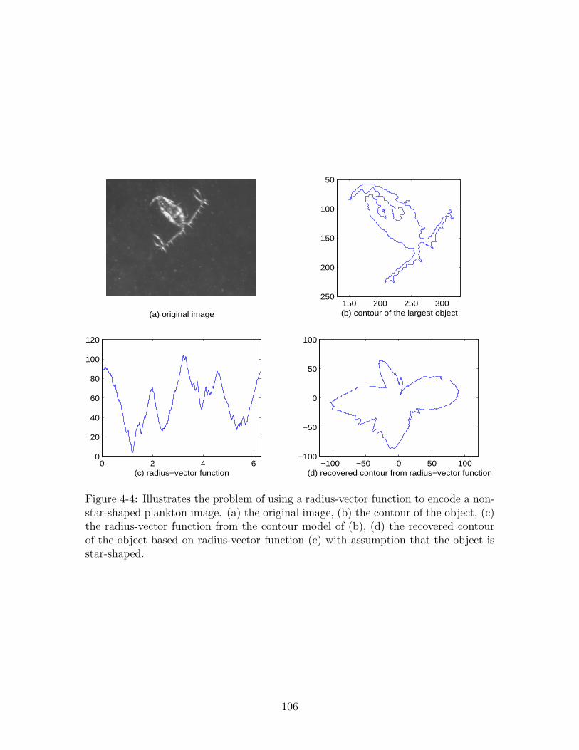
(a) original image150 200 250 300
50
100
150
200
250
(b) contour of the largest object
0 2 4 60
20
40
60
80
100
120
(c) radius−vector function−100 −50 0 50 100
−100
−50
0
50
100
(d) recovered contour from radius−vector function
Figure 4-4: Illustrates the problem of using a radius-vector function to encode a non-star-shaped plankton image. (a) the original image, (b) the contour of the object, (c)the radius-vector function from the contour model of (b), (d) the recovered contourof the object based on radius-vector function (c) with assumption that the object isstar-shaped.
106
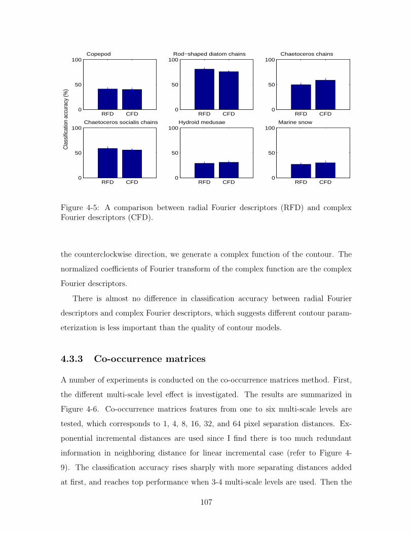
RFD CFD0
50
100Copepod
RFD CFD0
50
100Rod−shaped diatom chains
RFD CFD0
50
100 Chaetoceros chains
RFD CFD0
50
100 Chaetoceros socialis chains
C
lass
ifica
tion
accu
racy
(%)
RFD CFD0
50
100Hydroid medusae
RFD CFD0
50
100Marine snow
Figure 4-5: A comparison between radial Fourier descriptors (RFD) and complexFourier descriptors (CFD).
the counterclockwise direction, we generate a complex function of the contour. The
normalized coefficients of Fourier transform of the complex function are the complex
Fourier descriptors.
There is almost no difference in classification accuracy between radial Fourier
descriptors and complex Fourier descriptors, which suggests different contour param-
eterization is less important than the quality of contour models.
4.3.3 Co-occurrence matrices
A number of experiments is conducted on the co-occurrence matrices method. First,
the different multi-scale level effect is investigated. The results are summarized in
Figure 4-6. Co-occurrence matrices features from one to six multi-scale levels are
tested, which corresponds to 1, 4, 8, 16, 32, and 64 pixel separation distances. Ex-
ponential incremental distances are used since I find there is too much redundant
information in neighboring distance for linear incremental case (refer to Figure 4-
9). The classification accuracy rises sharply with more separating distances added
at first, and reaches top performance when 3-4 multi-scale levels are used. Then the
107
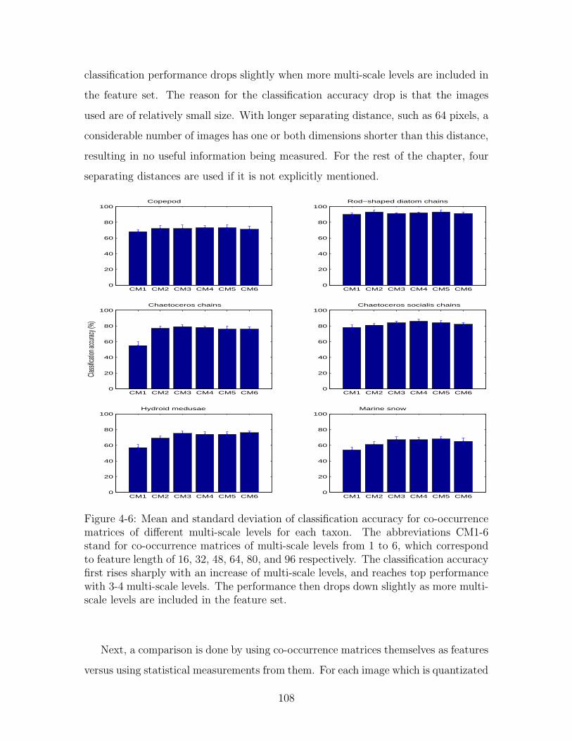
classification performance drops slightly when more multi-scale levels are included in
the feature set. The reason for the classification accuracy drop is that the images
used are of relatively small size. With longer separating distance, such as 64 pixels, a
considerable number of images has one or both dimensions shorter than this distance,
resulting in no useful information being measured. For the rest of the chapter, four
separating distances are used if it is not explicitly mentioned.
CM1 CM2 CM3 CM4 CM5 CM60
20
40
60
80
100Copepod
CM1 CM2 CM3 CM4 CM5 CM60
20
40
60
80
100Rod−shaped diatom chains
CM1 CM2 CM3 CM4 CM5 CM60
20
40
60
80
100 Chaetoceros chains
Classi
ficatio
n accu
racy (
%)
CM1 CM2 CM3 CM4 CM5 CM60
20
40
60
80
100 Chaetoceros socialis chains
CM1 CM2 CM3 CM4 CM5 CM60
20
40
60
80
100Hydroid medusae
CM1 CM2 CM3 CM4 CM5 CM60
20
40
60
80
100Marine snow
Figure 4-6: Mean and standard deviation of classification accuracy for co-occurrencematrices of different multi-scale levels for each taxon. The abbreviations CM1-6stand for co-occurrence matrices of multi-scale levels from 1 to 6, which correspondto feature length of 16, 32, 48, 64, 80, and 96 respectively. The classification accuracyfirst rises sharply with an increase of multi-scale levels, and reaches top performancewith 3-4 multi-scale levels. The performance then drops down slightly as more multi-scale levels are included in the feature set.
Next, a comparison is done by using co-occurrence matrices themselves as features
versus using statistical measurements from them. For each image which is quantizated
108
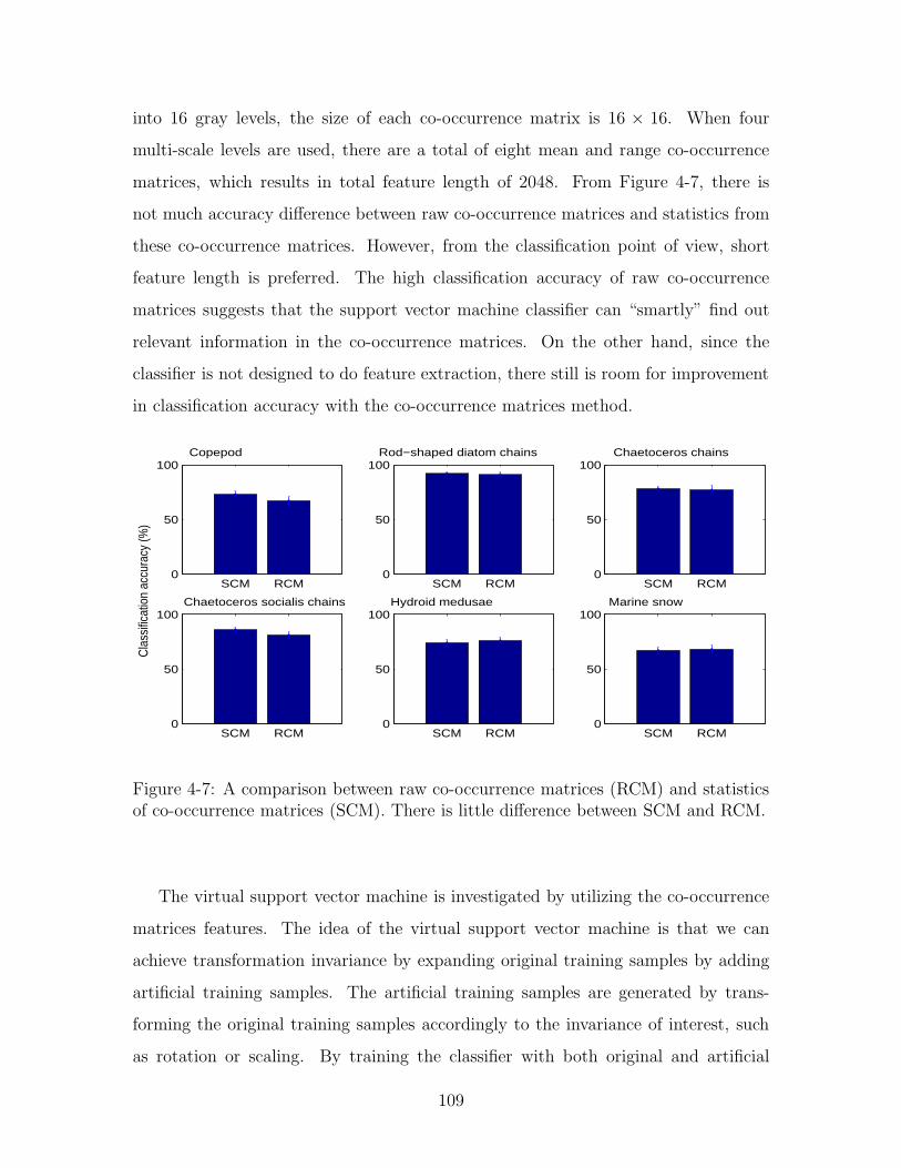
into 16 gray levels, the size of each co-occurrence matrix is 16 × 16. When four
multi-scale levels are used, there are a total of eight mean and range co-occurrence
matrices, which results in total feature length of 2048. From Figure 4-7, there is
not much accuracy difference between raw co-occurrence matrices and statistics from
these co-occurrence matrices. However, from the classification point of view, short
feature length is preferred. The high classification accuracy of raw co-occurrence
matrices suggests that the support vector machine classifier can “smartly” find out
relevant information in the co-occurrence matrices. On the other hand, since the
classifier is not designed to do feature extraction, there still is room for improvement
in classification accuracy with the co-occurrence matrices method.
SCM RCM0
50
100Copepod
SCM RCM0
50
100Rod−shaped diatom chains
SCM RCM0
50
100 Chaetoceros chains
SCM RCM0
50
100 Chaetoceros socialis chains
Cla
ssifi
catio
n ac
cura
cy (%
)
SCM RCM0
50
100Hydroid medusae
SCM RCM0
50
100Marine snow
Figure 4-7: A comparison between raw co-occurrence matrices (RCM) and statisticsof co-occurrence matrices (SCM). There is little difference between SCM and RCM.
The virtual support vector machine is investigated by utilizing the co-occurrence
matrices features. The idea of the virtual support vector machine is that we can
achieve transformation invariance by expanding original training samples by adding
artificial training samples. The artificial training samples are generated by trans-
forming the original training samples accordingly to the invariance of interest, such
as rotation or scaling. By training the classifier with both original and artificial
109

SCM CCM RCM0
50
100Copepod
SCM CCM RCM0
50
100Rod−shaped diatom chains
SCM CCM RCM0
50
100 Chaetoceros chains
SCM CCM RCM0
50
100 Chaetoceros socialis chains
Cla
ssifi
catio
n ac
cura
cy (%
)
SCM CCM RCM0
50
100Hydroids medusae
SCM CCM RCM0
50
100Marine snow
Figure 4-8: Virtual support vector machine test on the co-occurrence matricesmethod. SCM - statistics of co-occurrence matrices, CCM - statistics of co-occurrencematrices from original image and its complement, RCM - statistics of co-occurrencematrices from original image and resized images of 0.8 and 1.2. No accuracy gain isobtained by adding virtual samples in the training set.
samples with enough time, the hope is that the classifier will achieve transformation
invariance from the samples. Figure 4-8 is the result of the virtual support vector
machine test. There is no improvement in expanding the original training samples to
its complement and its resized version, which suggest that the co-occurrence matrices
feature has already achieved such invariance.
4.3.4 Edge frequency
The exponential distance interval spectrum works better than the linear distance
interval spectrum, while four direction formulation works better than two direction
formulation (Figure 4-9). The average classification accuracies of the linear distance
interval, the exponential distance interval with two directions, the exponential dis-
tance interval with four directions are 56.7%, 60.9%, and 65.5% respectively. The
classification accuracy for interested taxon ranges from 34.4% to 84.3% for linear dis-
tance interval, from 41.7% to 88.3% for two direction formulation, and from 49.0%
110

to 89.5% for four direction formulation.
EF1 EF2 EF30
50
100Copepod
EF1 EF2 EF30
50
100Rod−shaped diatom chains
EF1 EF2 EF30
50
100 Chaetoceros chains
EF1 EF2 EF30
50
100 Chaetoceros socialis chains
Cla
ssifi
catio
n ac
cura
cy (%
)
EF1 EF2 EF30
50
100Hydroid medusae
EF1 EF2 EF30
50
100Marine snow
Figure 4-9: A comparison of edge frequency features, where EF1 is EF spectrum withlinear distance interval from 1 to 40 pixels and two directions formula (horizontal &vertical, and diagonals), EF2 is EF with 7 exponential distance interval from 1 to 64and two directions formula (horizontal & vertical, and diagonals), EF3 is EF with7 exponential distance interval from 1 to 64 and four directions formula (horizontal,vertical and two diagonals). It is clear that exponential distance interval works betterthan the linear distance interval, and four direction formula works better than twodirection formula.
4.3.5 Run length
Basic run length statistics proposed by Galloway [52], and run length statistics ex-
tended by Chu et al. [22], and Dasarathy & Holder [29] are investigated (Figure 4-10).
The extended statistics have an average accuracy of 66.7%, while basic statistics have
an average accuracy of 60.6%. The classification accuracy for interested taxon ranges
from 57.0% to 78.4% for basic statistics, while from 64.5% to 83.6% for extended
statistics.
111

RL1 RL20
50
100Copepod
RL1 RL20
50
100Rod−shaped diatom chains
RL1 RL20
50
100 Chaetoceros chains
RL1 RL20
50
100 Chaetoceros socialis chains
Cla
ssifi
catio
n ac
cura
cy (%
)
RL1 RL20
50
100Hydroid medusae
RL1 RL20
50
100Marine snow
Figure 4-10: Comparison of run length methods. RL1 - run length statistics proposedby Galloway, 5 statistics from each run length matrix, total 20 features for 4 directions.RL2 - extended run length statisitcs by Chu et al., and by Dasarathy and Holder.11 statistics from each run length matrix, total 44 features for 4 directions. Theextended features give a slight better performance for all the taxa.
4.3.6 Pattern spectrum
Pattern spectrum as implemented by Vincent [162] (PS1) is compared with that
implemented by Meijster and Wilkinson [114] (PS2). PS2 is extended to include line
opening/closing spectra as well as area opening/closing spectra. PS1 outperforms PS2
on all the taxa except marine snow. The average classification accuracies for PS1 and
PS2 are 61.4% and 52.2% respectively. The classification accuracy for interested taxon
ranges from 49.8% to 85.3% for PS1, while from 36.9% to 77.8% for PS2 (Figure 4-11).
4.3.7 Wavelet transform
The classification accuracies for wavelet transform feature increase with use of more
multi-scale level at first, then change a little after 3-4 multi-scale levels are considered
(Figure 4-12). The average classification accuracy changes from 59.2% to 64.3% from
WL1 to WL7.
112

PS1 PS20
50
100Copepod
PS1 PS20
50
100Rod−shaped diatom chains
PS1 PS20
50
100 Chaetoceros chains
PS1 PS20
50
100 Chaetoceros socialis chains
Clas
sifica
tion
accu
racy
(%)
PS1 PS20
50
100Hydroid medusae
PS1 PS20
50
100Marine snow
Figure 4-11: Comparison between two implementations of pattern spectrum. PS1 -PS by Vincent, linear and pseudo opening and closing spectra, each has 40 elements,total feature length of 160. PS2 - PS modified from Meijster and Wilkinson, horizontaland vertical line opening and closing spectra, and area opening and closing spectra,each has 40 elements, total feature length of 240. PS1 outperforms PS2 on all thetaxa except marine snow.
WL1 WL2 WL3 WL4 WL5 WL6 WL70
20
40
60
80
100Copepod
WL1 WL2 WL3 WL4 WL5 WL6 WL70
20
40
60
80
100Rod−shaped diatom chains
WL1 WL2 WL3 WL4 WL5 WL6 WL70
20
40
60
80
100 Chaetoceros chains
Classif
ication
accur
acy (%
)
WL1 WL2 WL3 WL4 WL5 WL6 WL70
20
40
60
80
100 Chaetoceros socialis chains
WL1 WL2 WL3 WL4 WL5 WL6 WL70
20
40
60
80
100Hydroid medusae
WL1 WL2 WL3 WL4 WL5 WL6 WL70
20
40
60
80
100Marine snow
Figure 4-12: Multi-scale level test for wavelet transform features. WL1-7 stands forfeatures from wavelet transform with multi-scale level from 1 to 7.
113

4.4 Conclusion
Texture-based features are more important to classify field-collected plankton images
than shape-based features, even though shape-based features are extensively used in
the literature.
Multi-scale representation of texture features helps to improve the distinctive
power of texture features. Exponential incremental distance works better than linear
incremental distance. The optimal multi-scale level depends on the resolution and
size of the images. For this dataset, the optimal multi-scale levels are 3-4 levels.
Multi-scale co-occurrence matrices work best among all the feature methods tested.
The mean classification accuracy of 73% for seven taxa on independent testing data
sets is achieved using four multi-scale co-occurrence matrices.
114

Chapter 5
Co-Occurrence Matrices and
Support Vector Machine
In the previous chapter, I compared different feature presentation methods, and
demonstrated that multi-scale texture-based pattern presentation methods are more
suitable to classify field-collected images. In this chapter, I apply these findings and
develop a classification method, which utilizes texture-based features, multi-scale co-
occurrence matrices, and a support vector machine (COM-SVM) to classify the whole
data set and estimate the abundance of 6 major taxonomic groups. Such results are
compared against previous classification system with combined shape-based features
and neural network(CSF-NN) classifier[34]. Using texture-based features calculated
from multi-scale co-occurrence matrices alone reduces the classification error rate
from 39 to 28%. Subsequent plankton abundance estimates are improved by more
than 50% in regions of low relative abundance. This chapter was published in Marine
Ecology Progress Series[73].
This chapter is organized as follows. In Section 5.1, I describe the co-occurrence
matrices method. In Section 5.2, I discuss the support vector machine method. In
Section 5.3, I describe the feature extraction and classification used in this chapter.
The classification results are given in Section 5.4, followed by the conclusion in
Section 5.5.
115

5.1 Co-Occurrence Matrices
Spatial gray level co-occurrence provides second-order statistics from the images.
Julesz [85] first used first-order and second-order statistics in texture discrimination.
The co-occurrence method was first proposed by Haralick et al. [59] as a texture
feature and it has been widely used thereafter. It is based on estimation of the joint
probability distribution of pairs of pixels with gray level i and j, spatial distance d
and angle θ in an image. Each element in the co-occurrence matrix is the occurrence
of pairs of pixels having gray levels i and j and a certain spatial relationship in the
whole image (i.e., distance d and angle θ). Thus, for an image of L quantization level,
the size of its co-occurrence matrix is L × L. The number of co-occurrence matrices
is dependent on the number of different separation distances and quantized levels of
the angle. For computation efficiency, the angle is usually quantized to 45◦ or 90◦.
It is hard to select d without prior information. It is common to choose d = 1. In
my experiment, I have quantized angle to 45◦, which resulted in 4 different angles
(0, 45, 90, and 135◦), and chose d = 1, 4, 8, 16 pixels.
5.2 Support Vector Machines
Support Vector Machines (SVM) were proposed by Vapnik [160, 161] and have yielded
excellent results in a variety of data classification tasks. It is primarily a two-class
classifier and involves two steps. First, the feature vectors, x, of the training samples
are mapped into a high (potentially infinite) dimensional space, H. A hyperplane
then is constructed in order to separate the training samples in H. Different mappings
x 7→ Φ(x) ∈ H construct different SVMs.
The mapping Φ(·) is performed by a kernel function K(·, ·) which defines an inner
(dot) product in H. The decision function (i.e., the hyperplane), f , given by an SVM
is
f(x) = sgn(< w, Φ(x) > + b) = sgn(m
∑
i=1
αiyiK(xi, x) + b), (5.1)
where w and b define the orientation and translation of f , respectively, i is the
116
training sample index, y is class label, and α is a scalar.
The goal in training an SVM is to find the separating hyperplane which has the
maximal distance to the closest training samples in space H. This distance is called
the margin. These particular training feature vectors used to determine optimal
hyperplanes are called support vectors. In order to cope with non-separable cases,
a set of slack variables ξi ≥ 0 are introduced. If there are m training samples:
x1,x2, · · · ,xm with class label yi ∈ {−1, 1}, the classification reduces down to the
following optimization problem:
minimize LP (w, ξ) =1
2‖ w ‖2 +
C
m
m∑
i=1
ξi, (5.2)
with relaxed separation constraints,
yi(< φ(xi),w > +b) ≥ 1 − ξi, i = 1, · · · , m. (5.3)
where w is normal to the hyperplane, C is a scalar value that controls the tradeoff
between the empirical risk and margin width. The dual formulation is usually easy
to solve, and is defined as:
maximize LD(α) =
m∑
i=1
αi −1
2
m∑
i,j
αiαjyiyjK(xi, xj), (5.4)
subject to the constraints
m∑
i=1
αiyi = 0, 0 ≤ αi ≤ C, i = 1, · · · , m. (5.5)
There are three main ways to extend SVMs from 2-class to multi-class classifi-
cation: 1) The simplest is the one-versus-all approach [133] in which a set of binary
SVMs are trained to separate one class from the rest. The main drawback of this
approach is that the sample size is unbalanced, with the number of images in the
selected class typically being much less than the number of images not in that class.
2) Another method is the Error-Correcting Output Codes [39], in which a series of
117

binary problems are generated from a multiclass problem by splitting the original
set of classes into two subsets. This method appears promising but is untested for
plankton image data. 3) In the present study, I used a pairwise approach, where all
possible pairs of 2 classes were used to build binary SVMs. For the classification with
N classes, N(N−1)2
binary SVMs are needed. This yields 21 binary SVMs for our case
of 7 classes.
An important property of SVM is that the complexity of the classifier is charac-
terized by the number of support vectors instead of the dimension of the hyperspace
H. As a result, the SVM is less prone to over-fitting than other methods.
5.3 Feature Extraction and Classification
Each image was first quantized to 16 levels. The co-occurrence matrices were cal-
culated from 4 different angles (0, 45, 90, 135) and 4 different distances ( 1, 4, 8,
16 pixels). A frequency normalization was performed by dividing each entry in the
co-occurrence matrices by the total number of neighbor pairs. For example, for an
image of size M × N , when the relationship between nearest horizontal neighbors
is (d = 1, θ = 0◦), there will be a total of 2N(M − 1) nearest horizontal neighbor
pairs. For every four matrices with the same distance, the mean and range matrices
were calculated. Thus, for each image, eight co-occurrence matrices were computed.
The energy, contrast, correlation, variance, inverse-difference moment, and entropy of
these matrices[59] were calculated and used as feature vector elements. These features
were further normalized to have zero mean and unit standard deviation.
The Ohio State University (OSU) support vector machine (OSU-SVM) was used
to classify these feature vectors. The OSU-SVM was developed by Ma, Zhao, and
Anhalt for Matlab platform using Chang and Lin’s LIBSVM algorithm (Chang & Lin,
2001). It is available at http://www/ece.osu.edu/∼maj/osu svm. The OSU-SVM
uses decomposition in its optimization and a pair-wise approach to do multi-class
classification. Different kernels were tested on my data set. In my experiment, the
Gaussian radial basis function (RFB) performed best in terms of validation error.
118

The Guassian RBF kernel is defined as
k(x, y) = exp(−‖ x − y ‖2
2σ2),
where σ is a scalar value.
Two data sets were randomly picked from the working data set. These data sets
had 200 samples per taxon and were used to train and validate the SVM classifier,
respectively. Values of σ and the regularization constant C were optimized based
on the classification error found from tests with the validation data set. Values of
σ = 0.1, C = 50 gave the best classifier performance. Since the validation data set
was used to tune the classifier parameters, it is not valid to use them to testify the
classifier (i.e., generate confusion matrix). In this study, the classifiers are verified by
classifying the whole data set.
5.4 Classification results
I compared the performance of my COM-SVM system to the prior plankton clas-
sification system described in Chapter 3 [150, 34]. The COM-SVM yielded a 28%
reduction in recognition error rate (cf. Table 5.1 and Table 5.2, respectively). The
overall performance of the COM-SVM was 72% compared to 61% of the previous
system. The COM-SVM classifier performed better than the combined shape-based
features (moment invariants, Fourier descriptor, granulometry curve, and morpholog-
ical measurements) and neural network (CSF-NN) classifier for almost all the cate-
gories except the “other” category (Tables 5.1 and 5.2). This finding supports my
idea that for field-collected samples, texture-based features are more important than
global shape-based features in plankton classification, due to occlusion and nonlinear
illumination, or projection variance inherent in field-collected images. Most occlu-
sions occur when part of an organism is out of the image volume. Some occlusions
happen when part of an organism is darker than the rest because of the the nolin-
ear illumination. The global segmentation only segments part of the organism (cf.
119

Figure 4-3). The situation of nonlinear illunimation should be improved by using a
ring-illuminator in future instruments. A small amount of occlusion can also occur
when an out-of-focus organism is in the light path of an in-focus organism. This
situation only occurs when the concentration of the plankton is very high (≥ 10 ind.
ml−1).
Table 5.1: Confusion matrix for EN302, VPR Tow 7, based on the co-occurence ma-trix classifier using hold-out method. Column and row heading are coded as: C1,copepod; C2, rod-shaped diatom chains; C3, Chaetoceros chains; C4, Chaetocerossocialis colonies; C5, hydroid medusae; C6, marine snow; C7, ’other’; and Pd, proba-bility of detection. True counts (i.e. human counts) for a given taxa are given in thecolumns, while counts by automatic identification (i.e. computer counts) are given inthe rows. Correct identifications by the computer are given along the main diagonal,while the off-diagonal entries are the incorrect identification by the computer. Overallaccuracy for this classifier was 72%.
C1 C2 C3 C4 C5 C6 C7C1 4400 72 8 5 79 22 1081C2 96 3327 11 9 17 54 330C3 62 31 390 44 147 47 236C4 57 59 13 2100 47 267 390C5 231 10 29 15 1295 50 168C6 65 48 15 146 153 1146 137C7 1058 104 11 73 60 68 1977Pd 74 91 82 88 72 69 46
Although Culverhouse et al. [28] showed that human experts were far from perfect
for certain difficult classification tasks such as plankton identification, for simplicity,
we considered the human expert as a “perfect classifier” in this study. The effect
of training with contaminated training samples is a very interesting research topic.
Research on handwritten characters by Scholkopf & Smola [139] suggests that classi-
fier performance was not too sensitive to a small amount of contamination. Further
study is needed to decide how “clean” the training set needs to be to have a reliable
classifier(cf. classification stability, Chapter 4).
Testing the effects of different kernels and their parameters revealed that the SVM
classifier was robust to both kernel function type and parameters specific to the kernel
(cf. Table 5.3). For radial basis function (Gaussian kernel), the recognition rate was
120
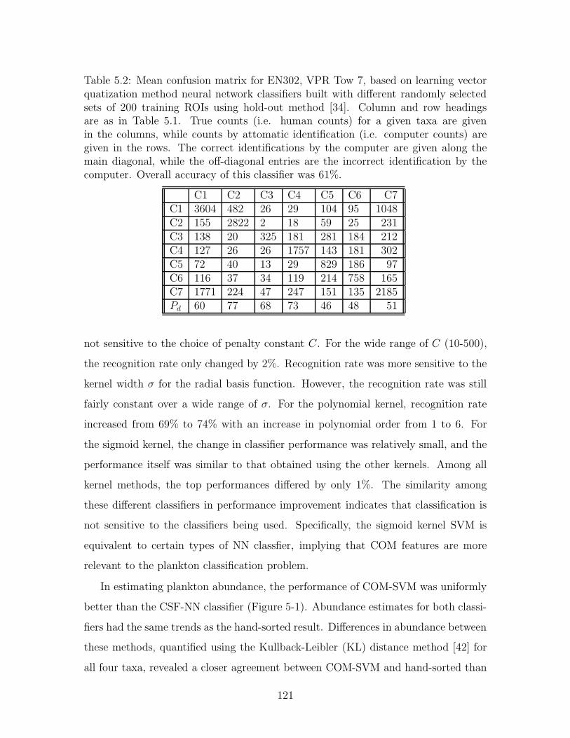
Table 5.2: Mean confusion matrix for EN302, VPR Tow 7, based on learning vectorquatization method neural network classifiers built with different randomly selectedsets of 200 training ROIs using hold-out method [34]. Column and row headingsare as in Table 5.1. True counts (i.e. human counts) for a given taxa are givenin the columns, while counts by attomatic identification (i.e. computer counts) aregiven in the rows. The correct identifications by the computer are given along themain diagonal, while the off-diagonal entries are the incorrect identification by thecomputer. Overall accuracy of this classifier was 61%.
C1 C2 C3 C4 C5 C6 C7C1 3604 482 26 29 104 95 1048C2 155 2822 2 18 59 25 231C3 138 20 325 181 281 184 212C4 127 26 26 1757 143 181 302C5 72 40 13 29 829 186 97C6 116 37 34 119 214 758 165C7 1771 224 47 247 151 135 2185Pd 60 77 68 73 46 48 51
not sensitive to the choice of penalty constant C. For the wide range of C (10-500),
the recognition rate only changed by 2%. Recognition rate was more sensitive to the
kernel width σ for the radial basis function. However, the recognition rate was still
fairly constant over a wide range of σ. For the polynomial kernel, recognition rate
increased from 69% to 74% with an increase in polynomial order from 1 to 6. For
the sigmoid kernel, the change in classifier performance was relatively small, and the
performance itself was similar to that obtained using the other kernels. Among all
kernel methods, the top performances differed by only 1%. The similarity among
these different classifiers in performance improvement indicates that classification is
not sensitive to the classifiers being used. Specifically, the sigmoid kernel SVM is
equivalent to certain types of NN classfier, implying that COM features are more
relevant to the plankton classification problem.
In estimating plankton abundance, the performance of COM-SVM was uniformly
better than the CSF-NN classifier (Figure 5-1). Abundance estimates for both classi-
fiers had the same trends as the hand-sorted result. Differences in abundance between
these methods, quantified using the Kullback-Leibler (KL) distance method [42] for
all four taxa, revealed a closer agreement between COM-SVM and hand-sorted than
121

Table 5.3: Performance of the classifier with different kernel widths (σ), regulationpenalty (C) and kernel types, where d is the polynomial degree and κ is the kernelcoefficient. The recognition rate on the independent test set is shown.
Gaussian kernel (C = 50) k(x, x′) = exp(−||x−x′||2
2σ2 )
σ 0.2 0.5 1 2 3 5 10Rate 63 69 72 75 75 73 70
Gaussian kernel (σ = 2) k(x, x′) = exp(−||x−x′||2
2σ2 )
C 10 20 50 100 200 500Rate 73 75 75 75 74 73
Polynomial kernel (C = 5) k(x, x′) = (< x, x′ >)d
d 1 2 3 4 5 6Rate 74 74 74 72 69 69
Sigmoid kernel k(x, x′) = tanh(κ < x, x′ > +θ)
κ 0.01 0.02 0.05 0.1 0.2 0.5Rate 69 71 73 74 72 60
between hand-sorted and CSF-NN (Table 5.4), reflecting the higher accuracy of the
COM-SVM method. In order to investigate the relative contribution of COM and
SVM in improving performance, the SVM classifier was trained using original fea-
tures. The abundance estimation of this classifier (CSF-SVM) was compared to that
of the original classifier (CSF-NN). The CSF-SVM classifier was found to perform bet-
ter than the CSF-NN classifier in regions of low abundance for Chaetoceros socialis
colonies. However, the CSF-SVM classifier gave underestimates in relatively high
abundance regions. In overall performance, the CSF-SVM classifier and CSF-NN
classifier were fairly similar (Figure 5-2). As discussed by Davis et al. [34], when the
relative abundance of a taxon is above 20-25%, the abundance estimation error due
to misclassification falls well within the natural variation for replicate plankton tows.
In areas of low relative abundance, accuracy of the abundance estimates is typically
much lower [34, 146]. The 28% reduction in recognition error results in a reduction in
abundance estimate error rate for Chaetoceros socialis colonies by more than 50% in
areas of low relative abundance (Figure 5-3). The reduction in abundance error rate
is due to the use of both COM and SVM. Positive values indicate improved perfor-
mance, while negative values indicate worse performance. COM-SVM out-performed
122

CSF-SVM in most cases, except in regions of low C. socialis abundance. The latter
performance difference was due to general underestimation by the CSF-SVM classifier
and consequent increase in C. socialis abundance in these regions. These observations
further support the idea that use of texture-based features (i.e. co-occurrence matrix)
is the main reason for performance improvement in our classification system.
5 10 15 20 250
1
2
3
4Copepods
5 10 15 20 250
1
2
3
4Rod−shaped diatom chains
5 10 15 20 250
1
2
3
4 Chaetoceros chains
Abs
olut
e a
bund
ance
(#
indi
vidu
als
/ lite
r)
5 10 15 20 250
1
2
3
4 Chaetoceros socialis colonies
Abs
olut
e a
bund
ance
(#
indi
vidu
als
/ lite
r)
5 10 15 20 250
1
2
3
4Hydroid medusae
Hour of Day(GMT)5 10 15 20 25
0
1
2
3
4Marine snow
Hour of Day(GMT)
manually sortedCSF−NN classifierCOM−SVM classifier
Figure 5-1: Comparison of 2 automated classifier with human expert classified resultsfor 6 dominant taxa along the tow timescale. CSF-NN, combined shape-based featuresand neural network; COM-SVM, co-occurrence features and support vector machine.The data are first binned into 10 second time intervals. A 1 hour smoothing windowis applied to the binned data.
The pair-wise approach was chosen in order to extend the binary SVM classifier
to the multi-class SVM classifier used in this study. Another approach using the
Error-Correcting Output Coding method [39] also appears to be very promising and
123
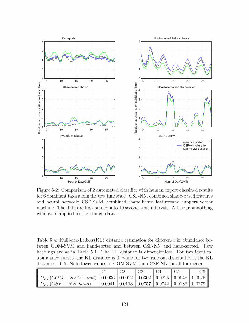
5 10 15 20 250
1
2
3
4Copepods
5 10 15 20 250
1
2
3
4Rod−shaped diatom chains
5 10 15 20 250
1
2
3
4 Chaetoceros chains
Abs
olut
e a
bund
ance
(#
indi
vidu
als
/ lite
r)
5 10 15 20 250
1
2
3
4 Chaetoceros socialis colonies
Abs
olut
e a
bund
ance
(#
indi
vidu
als
/ lite
r)
5 10 15 20 250
1
2
3
4Hydroid medusae
Hour of Day(GMT)5 10 15 20 25
0
1
2
3
4Marine snow
Hour of Day(GMT)
manually sortedCSF−NN classifierCSF−SVM classifier
Figure 5-2: Comparison of 2 automated classifier with human expert classified resultsfor 6 dominant taxa along the tow timescale. CSF-NN, combined shape-based featuresand neural network; CSF-SVM, combined shape-based featuresand support vectormachine. The data are first binned into 10 second time intervals. A 1 hour smoothingwindow is applied to the binned data.
Table 5.4: Kullback-Leibler(KL) distance estimation for difference in abundance be-tween COM-SVM and hand-sorted and between CSF-NN and hand-sorted. Rowheadings are as in Table 5.1. The KL distance is dimensionless. For two identicalabundance curves, the KL distance is 0, while for two random distributions, the KLdistance is 0.5. Note lower values of COM-SVM than CSF-NN for all four taxa.
C1 C2 C3 C4 C5 C6DKL(COM − SV M, hand) 0.0036 0.0022 0.0302 0.0225 0.0048 0.0075DKL(CSF − NN, hand) 0.0041 0.0113 0.0757 0.0742 0.0188 0.0279
124

5 10 15 20 25−100
−50
0
50
100Copepods
5 10 15 20 25−100
−50
0
50
100Rod−shaped diatom chains
5 10 15 20 25−100
−50
0
50
100 Chaetoceros chains
Red
uctio
n in
abu
ndan
ce e
rror
rat
e (%
)
5 10 15 20 25−100
−50
0
50
100 Chaetoceros socialis colonies
Red
uctio
n in
abu
ndan
ce e
rror
rat
e (%
)
5 10 15 20 25−100
−50
0
50
100Hydroid medusae
Hour of Day(GMT)5 10 15 20 25
−100
−50
0
50
100Marine snow
Hour of Day(GMT)
COM−SVM vesus SCF−NNSCF−SVM versus SCF−NN
Figure 5-3: Reduction in the relative abundance estimation error rate between COM-SVM and CSF-NN, and between CSF-SVM and CSF-NN. The positive value indicatesthat COM-SVM/CSF-SVM is better than CSF-NN, while the negative value indicatesCOM-SVM/CSF-NN is worse than CSF-NN.
125

is becoming an active research topic [3, 26, 122]. Further analysis of this method is
the subject of future study.
The new COM-SVM method only uses texture-based features (i.e. co-occurrence
matrices) to automatically classify plankton images. Shape-based features also carry
a substantial amount of information that can be used for classification. An attempt
was made to directly stack texture-based features and shape-based features into a
single feature vector, and train the classifier on this single feature vector (with and
without principal component analysis). Only a very limited improvement (less than
1% ) in recognition rate was obtained. This method of combining features was only
one approach, and further research is needed to determine whether other methods
(such as weighting each individual feature by its discriminative power) for combining
features may yield improved identification accuracy. Given the growing trend toward
optical imaging of marine biota, new methods of automatic identification are needed
to improve classification accuracy. The texture-based method presented here can be
used for a wide-variety of image classification problems, since it is not sensitive to
occlusion and lighting gradients and is independent of shape-based features.
5.5 Conclusion
In this chapter, I have used texture-based feature, co-occurrence matrices, to classify
plankton images taken in the field using the VPR. This method had 72% overall
recognition rate compared to 61% for a previous recognition system that used shaped-
based features. Shape-based features are the primary ones currently used in automatic
plankton recognition systems due to their early success on plankton images taken in
the laboratory. Texture-based features have been found to work better for field-
collected images of plankton because they are less sensitive to occlusion, non-uniform
lighting, and projection variance.
SVM was used to train the classifier. Classifier performance was not sensitive to
kernel type or to the exact parameter values used for specific kernels. In Chapter
3, we know that selection of representative training samples is an important factor.
126

In order to accurately assess classifier performance, a random set of training samples
from the field is recommended.
Multi-scale texture features are captured with multiple separation distances. Scale
invariance is achieved by normalization of co-occurrence matrices. Rotation invari-
ance is achieved by using only the range and mean co-occurrence matrices.
Continued improvements in accuracy of automatic image recognition methods will
enable wider use of this powerful approach. The growing use of underwater optical
imaging methods requires more emphasis on development and improvement of new
automatic identification techniques.
The method described here is a step toward the long term goal of highly-accurate
automatic identification of plankton from optical imaging systems.
127

128

Chapter 6
Dual classification system and
accurate plankton abundance
estimation
In the previous chapter, I demonstrated that using features from multi-scale co-
occurrence matrices can improve the plankton classification significantly. The auto-
matic classification results in general yield very good agreement with those obtained
with manually sorted results. However, in regions of relative low abundance or for
a taxon with relative low abundance, the classification is not accurate enough to
estimate taxonomic group abundance. In this chapter, I have developed a dual clas-
sification method to cope with these two situations. The dual-classification system
developed a rejection metric obtained by voting with 2 classifiers: 1) an NN classifier
built from shape-based features and 2) an SVM classifier built from texture-based
features. Both classifiers must agree on the identification of an image for it to be
considered true, otherwise it is classified as “unknown”. Abundance estimation from
the dual-classification system was corrected based on detection and false-alarm rates.
After correction, the abundance estimation from the automatic classification system
agreed very well with that derived from manually sorted results. This chapter was
published in Marine Ecology Progress Series[74].
This chapter is organized as follows. The dual-classification system is described in
129
Section 6.1. The dual-classification results are compared against single classification
results in 6.2. A short conclusion is made in Section 6.3
6.1 Dual classification system description
6.1.1 Pattern representations
Five different types of features have been used in the dual-classification system, includ-
ing shape-based features (moment invariants, morphological measurements, Fourier
descriptor and granulometry curves) and texture-based features (co-occurrence ma-
trix).
Moment invariants
Moment invariants, introduced by Hu [72], are based on normalized central moments,
and are translation, rotation, and scale invariant. They have been widely used in
plankton identification [82, 81, 150, 149, 34, 106].
Morphological measurements
Jeffries et al. [82, 81] first used 7 morphological measurements as features to iden-
tify zooplankton. The concept of using morphological measurement as features in
plankton recognition has been commonly accepted ever since then [34, 106]. In this
chapter, 6 morphological measurements were used as part of the shape-based feature
set: 1) a shape factor based on the perimeter and area of the object; 2) a ratio of
maximum and minimum principal moments of the object; 3) a ratio of longest and
shortest dimensions of the bounding box surrounding the object; 4) a ratio of the
width at center of the object to shortest dimension of the bounding box; 5) a ratio
of the left 1/4-width of the object to shortest dimension of the bounding box of an
object; 6) a ratio of the right 1/4-width of the object to shortest dimension of the
bounding box [34].
130
Fourier descriptors
Fourier descriptors (FD) are well-studied invariant features used to describe the con-
tour of an object. Depending on what functions are used to describe the contour, FDs
can be grouped into 3 major categories, namely tangent-angle FDs [175] , complex
FDs [57], and elliptic FDs [94]. FDs are the Fourier coefficients when the contour
function is approximated by a Fourier series. Normalized FDs were used as features
to classify plankton images [82, 81]. In this study, I used a centroidal radius-vector
function (distances from the centroid to perimeter pixels) as the contour model1. The
first 64 elements of the normalized power spectrum, obtained from the Fourier trans-
form of centroidal radius-vector function were used as a feature set [150, 149, 34].
These elements were also translation, rotation, and scale invariant.
Granulometry
The concept of granulometry was introduced by Matheron [112] to study size distri-
bution of binary images. The operation involves a series of openings/closings with
structuring elements of increasing/decreasing size [140]. Tang et al. [150] first used
granulometry features to classify plankton images. They found that the granulom-
etry was more powerful in discriminating plankton images than common moment
invariants and Fourier descriptors. However, these operators are computationally
expensive. Fast algorithms [162, 114] were developed for very limited structural el-
ements. In this chapter, Vincent’s algorithm [162] was used to calculate the linear
opening and closing spectra, as well as pseudo-opening and -closing spectra. Each
spectrum has 40 elements, resulting in 160 features for granulometry.
Co-occurrence matrix
Gray level co-occurrence matrices(GLCM) were first proposed by Haralick et al. [59]
as a texture feature to classify satellite images. It is based on estimation of the joint
1As discussed in Chapter 4, radius-vector functions are only suitable for star-shaped contourmodels. Most plankton images are not star-shaped. As shown in Chapter 4, the difference betweendifferent contour models are very small. To be consistent with earlier works, radius-vector functionswere used in this study.
131
probability distribution of pairs of pixels with gray-scale level i and j, spatial distance
d, and angle θ in an image. Hu & Davis [73] first used GLCM to classify plankton
images. They concluded that these texture-based features were more useful for clas-
sifying field-collected plankton images, due to occlusion, non-linear illumination and
projection variance of the images.
6.1.2 Feature extraction
Shape-based features
All the shaped-based features were stacked into 1 feature vector. The features in-
cluded 7 moment invariants, 6 morphological measurements, 64 Fourier descriptor
coefficients, and 160 granulometry measurements [34]. Each feature element was nor-
malized to have zero mean and unit standard deviation. Principal component analysis
was applied on the feature vector to calculate dominant eigenvectors. The first 30
features associated with the largest eigenvalues were saved as the feature vector, and
corresponding feature vectors were saved as a transformation matrix [150].
Texture-based features
Four different distance (1, 4, 8, 16 pixels) pairs and four different angles (0, 45, 90, 135◦)
were used to generate co-occurrence matrices. For each separation distance, there
were 4 co-occurrence matrices from 4 different angles. Only the mean and range of
these matrices were used to achieve relative rotation invariance. Normalization was
also applied to the resulting matrices to achieve scale invariance. The angular second
moment (energy), contrast, correction, variance, inverse-difference moment, entropy,
sum entropy, and difference entropy of these matrices [59, 73] were calculated and
used as feature vector elements. Each feature element was further normalized to have
zero mean and unit standard deviation. For each image, 64 features were used [73].
132

6.1.3 Classifiers
The learning vector quantization neural network classifier and support vector machine
classifier were used in this study.
Learning vector quantization
Learning vector quantization (LVQ) is a supervised version of vector quantization.
Its objective is to learn a set of prototypes (codebooks) which best represent each
class. We implemented it with an artificial neural network [149, 34]. LVQ neural
network (LVQ-NN) is a method to divide n-dimensional feature space into different
taxonomic regions by fitting neurons to the training data. The neural network has 2
layers, namely a competitive layer and a linear output layer. The complexity of the
neural network (prototypes of subclass, number of neurons) was based on the number
of training samples and the number of classes in the classifier. For the 200 samples per
taxon, I used 20 neurons per taxon for the competitive layer. The number of output-
layer neurons was equal to the number of taxa. The weights of the neurons for each
class were initialized to the mean of the training feature vectors for that class plus a
small random value. The network was trained by randomly presenting the training
samples to the network. For a given training sample, the nearest neuron (winning
neuron) was found (i.e. shortest Euclidean distance between the training samples to
all the neurons in feature space). The taxon assigned to this nearest neuron was the
“predicted” taxon of the neuron network. If the prediction was correct, the weights
of this winning neuron (prototype) were updated in such a way to move that neuron
a step closer to the training sample in the feature space. Otherwise, the weights
of the winning neuron were updated such that it was pushed a step away from that
sample in the feature space. The learning rate (step size) was preset from the trade-off
between the training time and the training error. A small learning rate was usually
associated with long training time and small training error, while a large learning rate
was usually associated with short training time and big training error. Over-training
was avoided by using number of neurons and epoches established in Chapter 3.
133
Support vector machine
The support vector machine (SVM) is a margin-based linear machine. It was first
proposed by Vapnik [160, 161]. Instead of using neurons, the basic idea of SVM is to
find a hyperplane which separates the training samples with maximum margin. The
capacity of linear SVM is often limited. In order to deal with the non-linear problem,
an intermediate step is taken to map original features to a much higher dimensional
space; a hyperplane is then constructed on that high space. The mapping step is
usually time consuming. The trick of nonlinear SVM is to pick certain mapping func-
tions which satisfy Mercer’s condition so that the mapping is equivalent to applying
a kernel function on the original features. In these cases, the mapping is not neces-
sary. Nonlinear SVM is solved exactly like linear SVM, except the original feature
vector is replaced by a kernel function of the feature vector. SVM is closely related
to structural risk minimization and regularization theory. It has shown a nice gener-
alization property and resistance to over-training in a number of real-world problems
[118, 37, 92, 117, 73]. SVM is primarily a binary classifier. Three approaches are
often used to extend SVM to multi-class case, namely one-vs-all approach, pairwise
approach, and error-correcting output codes approach. In the last chapter, I showed
that the SVM classifier was not very sensitive to kernel types and kernel parameters.
In this chapter, I chose a linear kernel function to avoid extra labeled validation sam-
ples which were needed in kernel parameter selection. The pairwise approach was
used, since it yielded balanced training in this case [73].
6.1.4 Dual classification system
The schematic diagram of the dual classification system is shown in Figure 6-1. During
the training phase, two classifiers were built in parallel. An LVQ-NN classifier was
built from shape-based features as discussed in the feature extraction section. At the
same time, an SVM classifier was built using texture-based features from the same
training samples. In the classification phase, shape-based and texture-based features
were calculated from all the samples. An LVQ-NN classifier made the identification
134

based on shape-based features, while an SVM classifier made the identification based
on texture-based features. In the end, a classifier committee was called. If the labels
predicted by the two classifiers belonged to the same class, the sample was labeled as
that class. Otherwise, the sample was labeled as “unknown”.
Training
Classification
All theSamples
Shape-basedFeatures
Texture-basedFeatures
LVQ-NNClassifier
SVMClassifer
C1=C2 ?
C1
C2Yes
Label =’C1’
No
Label = ’unknown’
TrainingSamples
Shape-basedFeatures
LVQNN
LVQ-NNClassifier
Texture-basedFeatures SVM SVM
Classifier
Figure 6-1: Schematic diagram of dual-classification system. LVQ: learning vectorquantization; NN: neural netowork; SVM: support vector machine
135

6.1.5 Classification performance evaluation and abundance
correction
Confusion matrix
The confusion matrix is used to assess the accuracy of automatic classification. The
number of images manually sorted by a human is given in the columns ( 1 column
per taxon), while the number of images automatically classified by a computer is
given in the rows (1 row per taxon). Diagonal elements correspond to agreement
between human and machine. In this chapter, the confusion matrix of the dual-
classification system was built in the following way. First, a 7 × 6 matrix was built
from a set of training images (200 per taxon) for 6 dominant taxa (Table 6.1) using
the leave-one-out method (cross-validation) [34]. The 7th row in this matrix contains
the “unknown” counts. Second, 200 images that had been manually sorted into an
“other” category were classified using the dual-classification system to fill in the 7th
column2. The resulting 7 × 7 matrix was used as the confusion matrix for the dual-
classification system (i.e. Table 6.1).
From the matrix, some simple indexes of classifier performance can be calculated.
The most used indexes are probability of detection (also known as sensitivity or
probability of true positives), and probability of false alarm (also known as probability
of false positives). The probability of detection, PD, measures the probability that the
classification system will label correctly for each class given the object belongs to that
class, i.e. PD = true positive counts/(true positive counts + false negative counts).
The probability of false alarm is the probability that an image will be classified as a
given taxon when it does not actually belong to that taxon. Another related concept
is specificity, SP[6], which is the probability that a classifier’s prediction is correct
for each taxon, i.e. SP = true positive counts /(true positive counts + false positive
counts). The probability of detection and specificity of each taxon were calculated
from the confusion matrix to correct the abundance estimation.
2The last classifier built in leave-one-out method was used.
136

Table 6.1: Confusion matrix of the dual-classification system, using the leave-one-outmethod. Randomly selected images (200 per category) from EN302 VPR tow 7 wereused to build the confusion matrix. C1: copepods, C2: rod-shaped diatom chains,C3: Chaetoceros chains, C4: Chaetoceros socialis colonies, C5: hydroid medusae, C6:marine snow, C7: other, C7*: unknown, PD: probability of detection (%), SP =specificity (%). NA: not applicable. True counts (i.e. human counts) for a given taxaare given in the columns, while counts by classification system are given in the rows.Correct identifications by the computer are given along the main diagonal, while theoff-diagonal entries are the incorrect identification by the computer. All data arecounts, except in the last row and last column, which are percent values. Althoughimages from the “other” category are not needed to train the dual-classification sys-tem, they are necessary to evaluate it.
C1 C2 C3 C4 C5 C6 C7 SPC1 146 0 3 2 1 2 59 69C2 2 176 2 0 1 1 13 90C3 0 0 122 1 3 1 2 95C4 0 0 0 145 2 8 12 87C5 0 0 5 0 111 6 4 88C6 1 0 0 3 4 98 4 89C7* 51 24 68 49 78 84 106 23PD 73 88 61 73 56 49 53 NA
137

Abundance correction
If PD and SP of a classification system for each taxon are always the same, plank-
ton abundance estimated from the classification system will be perfect although the
classfication system itself is not perfect. In reality, PD and specificity may change
for different-sized evaluation data sets. In particular, the specificity of a taxon is
positively related to the relative abundance of that taxon. However, if the variation
in PD and SP of a classification system for each taxon is relatively small in the study
area, we can automatically correct the abundance estimation from the classification
system using the following steps: 1) estimate PD and SP for each taxon from the
confusion matrix; 2) scale the abundance estimation from the classification system
for each taxon by the ratio SP/PD for that taxon. The manual correction method
discussed in Davis et al. [34], involves removing all false alarms manually from the
classification results. In that case, the specificity of each taxon was unity, and the
correction factor for each taxon was 1/PD. This correction method is different from
the statistical correction method discussed in Chapter 3 [146].
6.2 Classification results
The first 25 images classified as copepods and Chaetoceros socialis colonies by the
dual classification system and by the single neural network classifier [34] are shown
in Figure 6-2. For the taxa with high relative abundance (i.e. copepods), the perfor-
mance of dual-classification and single classifier is very similar, which implies the two
classification systems have very close probability of detection. On the other hand, for
taxa with lower relative abundance (i.e. C. socialis), the dual classification system
has a far lower false alarm rate (Figure 6-2). The dual classification system has much
higher specificity for C. socialis in regions of low relative abundance (cf. Table 6.1,
6.2). In other words, the dual classification system makes the specificity less variable
with changes in relative abundance of a taxon, which makes automatic correction of
classification results possible (Tables 6.1, and 6.2).
Abundance estimation of 6 dominant taxa were compared between manually
138

A B
C D
Figure 6-2: Automatically classified images: comparison of results for(A,C) dual-classification system and (B,D) single neural network classifier. The first 25 imagesclassified as (A,B) copepods and (C,D) Chaetoceros socialis by the dual-classificationsystem and LVQ-NN classifier are shown. For taxa having relatively high abundance,such as copepods, both systems yield very similar results (21 out of 25 were the same).In contrast, for taxa having relatively low abundance, such as low-abundance regionsof C. socialis, the dual-classification system has much higher specificity (fewer falsealarms).
139

Table 6.2: Confusion matrix of the single LVQ-NN classifier, using the leave-one-out method. Images used were the same as those in Table 6.1. Abbreviations as inTable 6.1. All data are counts, except in the last row and last column, which arepercent values.
C1 C2 C3 C4 C5 C6 C7 SPC1 132 8 16 2 16 7 54 56C2 6 171 1 4 7 5 20 80C3 7 1 123 10 23 22 11 62C4 6 2 14 153 5 20 14 72C5 5 5 13 4 105 21 9 65C6 9 3 20 17 34 109 15 53C7 35 10 13 10 10 16 77 45PD 66 86 62 77 53 55 39 NA
sorted, dual classification with automatic correction, single NN classifier of origi-
nal feature with manual correction [34](Figure 6-3). The manual correction method
[34] requires manual removal of false negative images from the automatically classi-
fied results for each taxon. The result was then further corrected by the probability
of detection which was estimated from Table 6.2. The automatic correction method
estimated probability of detection and specificity for each taxon from the confusion
matrix (Table 6.1), and used the correction factor discussed in the section 6.1.5.
Except for the copepod category, the manually sorted, manually corrected and
dual classification curves lie almost on top of each other (Figure 6-3). The high
agreement between manually corrected and manually sorted results for copepods is
due to the incorrect assumption that the human-sorted results were perfect and in-
variant. For this case, false negative samples were determined using a lookup table
from manually sorted images (i.e. no variations between manually corrected and
manually sorted results) rather than by manually correcting the classification result
as discussed by Davis et al.[34]. The high agreement between manually sorted and
manually corrected results of copepods abundance is an artifact of such a treatment.
In fact, among the manually sorted images, there is some overlap between copepods
and the “other” category due to ambiguity in appearance of some of the “other”
images, which may actually have been copepods oriented in such a way as to make
140

5 10 15 20 250
1
2
3
4Copepods
5 10 15 20 250
1
2
3
4Rod−shaped diatom chains
5 10 15 20 250
1
2
3
4 Chaetoceros chains
Abs
olut
e a
bund
ance
(#
indi
vidu
als
/ lite
r)
5 10 15 20 250
1
2
3
4 Chaetoceros socialis colonies
Abs
olut
e a
bund
ance
(#
indi
vidu
als
/ lite
r)
5 10 15 20 250
1
2
3
4Hydroid medusae
Hour of Day(GMT)5 10 15 20 25
0
1
2
3
4Marine snow
Hour of Day(GMT)
manually sorteddual classificationmanually corrected
Figure 6-3: Comparison of dual-classification, and manually corrected single NN clas-sification with human expert classified results for 6 dominant taxa along the towtimescale. The data are first binned into 10 second time intervals. A 1 hour smooth-ing window is applied to the binned data.
141

identification by a human difficult.
According to the study by Culverhouse et al. [28], trained personnel can be ex-
pected to achieve 67 to 83% self-consistency in difficult labeling tasks. Our copepods
category should belong to this case. That is to say, if a human labels all 20,000+
images a second time, the copepod abundance estimation between the two human
results is likely to differ. The mean abundance estimation for copepods between au-
tomatically classified and manually sorted results is very close. The uncertainty in
the manually sorted abundance estimation is comparable to the abundance difference
between automatic and manually sorted results.
Abundance estimation of 6 dominant taxa were compared between 3 automatic
classifiers (dual-classification, single NN classifier without correction, SVM classifier
from co-occurrence feature) and manually sorted results (Figure 6-4). For taxa in
high relative abundance regions, the 3 automatic classification systems agree very
well with manually sorted results. However, for taxa having low relative abundance
or taxa having low relative abundance regions, the reduction of the abundance er-
ror rate is marked (Figure 6-4). Chaetoceros chains make up less than 2.5% of total
plankton in this tow. The abundance estimation error of the dual-classification sys-
tem is uniformly less than 50% along the tow path, which is smaller than the natural
variation for replicate plankton tows [171, 34]. In the regions of extremely low rel-
ative abundance (e.g. Figure 6-3, hour 8 and 12, Chaetoceros socialis colonies), the
dual classification system estimates the abundance significantly higher than manually
sorted or manually corrected abundance.
The reduction in abundance error rates of the dual classification system com-
pared to the single NN classifier [34], the SVM classifier with co-occurrence matrices
[73], and manual correction [34] are given in Figure 6-5. For copepods, the manu-
ally corrected result outperforms other methods. As discussed above, this difference
is not significant, due to low confidence of the manually sorted result. For rod-
shaped diatom chains, the performances of dual classification, manually corrected,
and COM-SVM are very similar. They all outperform the single NN classifier. Dual
classification has a significant reduction in abundance error compared to OF-NN and
142
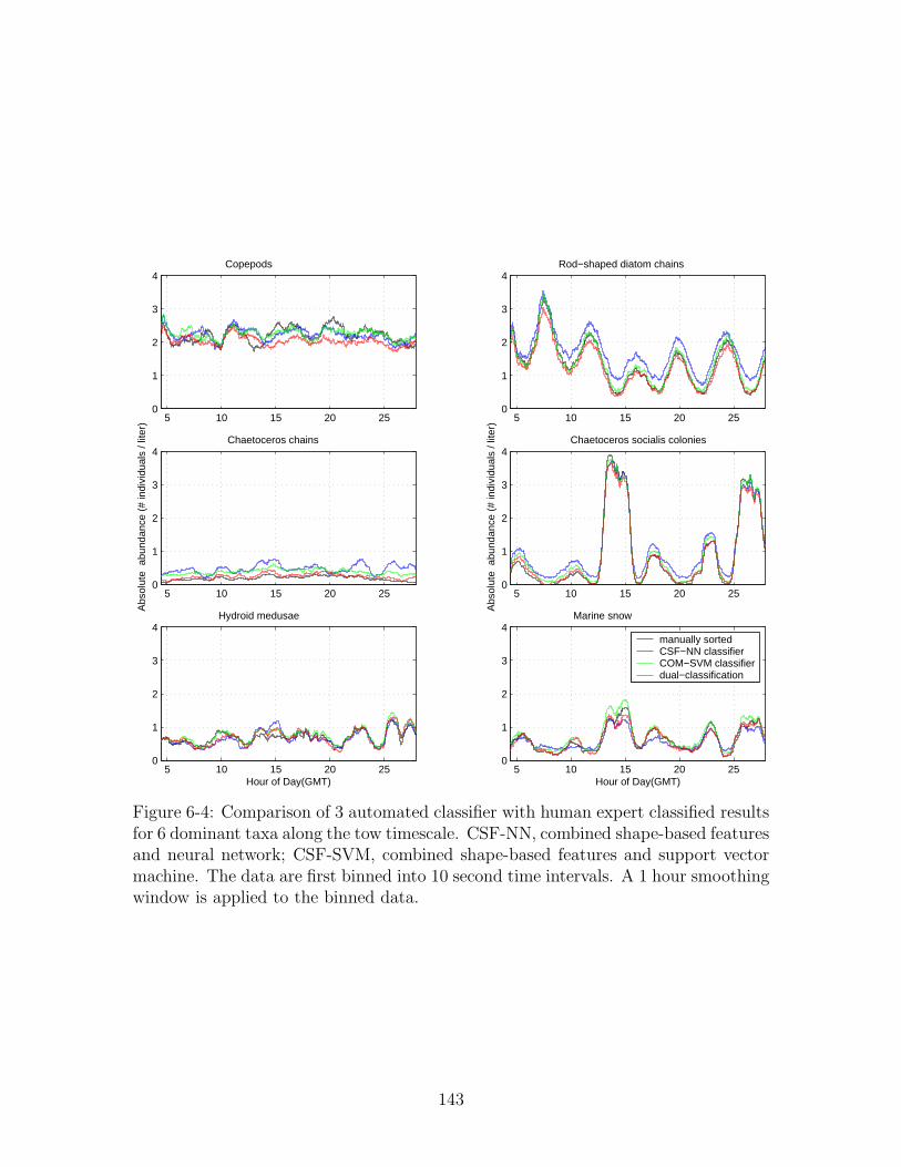
5 10 15 20 250
1
2
3
4Copepods
5 10 15 20 250
1
2
3
4Rod−shaped diatom chains
5 10 15 20 250
1
2
3
4 Chaetoceros chains
Abs
olut
e a
bund
ance
(#
indi
vidu
als
/ lite
r)
5 10 15 20 250
1
2
3
4 Chaetoceros socialis colonies
Abs
olut
e a
bund
ance
(#
indi
vidu
als
/ lite
r)
5 10 15 20 250
1
2
3
4Hydroid medusae
Hour of Day(GMT)5 10 15 20 25
0
1
2
3
4Marine snow
Hour of Day(GMT)
manually sortedCSF−NN classifierCOM−SVM classifierdual−classification
Figure 6-4: Comparison of 3 automated classifier with human expert classified resultsfor 6 dominant taxa along the tow timescale. CSF-NN, combined shape-based featuresand neural network; CSF-SVM, combined shape-based features and support vectormachine. The data are first binned into 10 second time intervals. A 1 hour smoothingwindow is applied to the binned data.
143

COM-SVM, while it is close to the manually corrected results. It is the same case for
C. socialis colonies. The performance disagreement occurs in the regions of extremely
low relative abundance. As discussed by Benfield et al. [9], these regions could be the
limits of the optical sampling method (i.e., high magnification VPR camera used).
The performance of four different methods on hydroid medusae and marine snow is
very close. The dual classification method performs slightly better for marine snow,
while the manually corrected method is better for hydroid medusae.
The advantage of using the dual-classification system is to reduce the false alarm
rate of each taxon to such a low level that the variation of specificity for each taxon
is low in the whole study region (Figure 6-6). This makes fully automatic correction
possible. The dual-classification system substantially decreases the probability of
false alarm, while only slightly reducing the probability of detection. By rejecting
a small portion of the images as “unknown”, identifications are made by the dual-
classification system with higher confidence. Thus, it is not necessary to classify all
the images into taxonomic groups to achieve better abundance estimation.
In this chapter, I present one way to integrate shape-based features with texture-
based features. Other approaches to incorporate shape-based features to texture-
based features are certainly possbile. In the simplest example, all available features
are stacked into 1 feature vector and used in training an SVM or LVQ-NN classifier
as I did for combining shape-based features. I have found that such an approach
is not efficient, and that the result is almost identical to the COM-SVM method. I
have also tried more sophisticated approaches to reduce feature dimension without
losing discriminant power, but have thus far met with little success. Such approaches
require further research.
A dual-classification system utilizes a greater range of variation in feature sets and
classifiers. The second classifier provides additional information that the first classifier
alone does not possess. It is certainly possible to use 1 type of classifier (e.g. SVM or
LVQ-NN) with all types of features or 1 type of feature for both classifiers. However,
the variability gained by the dual-classification system using different features and
different classifers would be reduced.
144
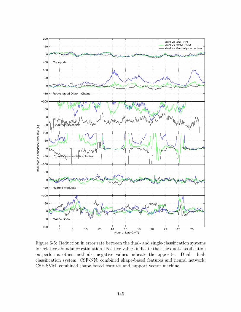
6 8 10 12 14 16 18 20 22 24 26−100
−50
0
50
Marine Snow
Hour of Day(GMT)
−100
−50
0
50
Hydroid Medusae
−100
−50
0
50
Chaetoceros socialis colonies
Red
uctio
n in
abu
ndan
ce e
rror
rate
(%)
−100
−50
0
50
Chaetoceros chains
−100
−50
0
50
Rod−shaped Diatom Chains
−100
−50
0
50
100
Copepods
dual vs CSF−NNdual vs COM−SVMdual vs Manually correction
Figure 6-5: Reduction in error rate between the dual- and single-classification systemsfor relative abundance estimation. Positive values indicate that the dual-classificationoutperforms other methods; negative values indicate the opposite. Dual: dual-classification system, CSF-NN: combined shape-based features and neural network;CSF-SVM, combined shape-based features and support vector machine.
145
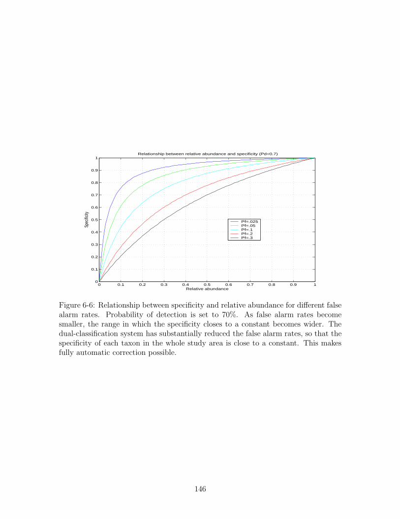
0 0.1 0.2 0.3 0.4 0.5 0.6 0.7 0.8 0.9 10
0.1
0.2
0.3
0.4
0.5
0.6
0.7
0.8
0.9
1
Relative abundance
Spec
ificity
Relationship between relative abundance and specificity (Pd=0.7)
Pf=.025Pf=.05Pf=.1Pf=.2Pf=.3
Figure 6-6: Relationship between specificity and relative abundance for different falsealarm rates. Probability of detection is set to 70%. As false alarm rates becomesmaller, the range in which the specificity closes to a constant becomes wider. Thedual-classification system has substantially reduced the false alarm rates, so that thespecificity of each taxon in the whole study area is close to a constant. This makesfully automatic correction possible.
146
The difficulty of general object classification may be overlooked because humans
are so good at visual classification of objects. We take for granted our ability to
identify facial images without considering the millions of years of evolution involved.
On the other hand, a computer is taught in less than 1 hour to identify plankton
images that suffer from projection variance, occlusion, non-uniform illumination, and
noise, using 200 training images per taxon. The assessment study in Chapter 3 [34]
revealed the difficulty level of this data set. I showed that the 90% + accuracy on
a selected subset of these data [150] only yielded 60% accuracy on the entire data
set. Although humans are able to identify some of the images in this data set to
a higher level of taxonomic group, the dual-classification method presented in this
chapter yields abundance estimation almost as accurate as those of human experts.
6.3 Conclusion
In this chapter, I used a dual-classification system by building an SVM classifier on
texture-based features (co-occurrence matrices) and an LVQ-NN classifier on shape-
based features (moment invariants, Fourier descriptors and granulometry) to jointly
identify over 20,000 VPR images. A confusion matrix was built from training sam-
ples. Sensitivity and specificity of the classification system were calculated from the
confusion matrix to correct the abundance estimation. After correction, the dual-
classification system reliably estimated the abundance of a taxon even when its rel-
ative abundance was as low as 2.5%. In regions of relatively low abundance, the
dual-classification system reduced the abundance estimation error by 50 to 100%
compared with previous methods. Because it is fully automatic, this method can be
used for real-time applications, as our previous methods discussed in Chapter 3 and
5 [34, 73].
147

148
Chapter 7
Conclusions and future work
The ultimate goal of this thesis is to build an automatic classification system which
can automatically obtain fine-scale abundance estimation of different taxonomic groups
from the Video Plankton Recorder. A statistical machine learning approach was used
to train the classification system. The major contributions of this thesis include
constructing a large real-world labeled data set, developing real-time focus detection
algorithms and evaluating their performance on the recorded VPR video, investi-
gating different pattern representation methods on this large data set, assessing an
existing learning vector quantization neural network classification system on this data
set in a systematic way, extracting features from multi-scale co-occurrence matrices,
designing different classification schemes, and proposing different correction methods
to correct classification results.
This is the first study of taxa-specific abundance estimation with machine learning
and pattern recognition on field-collected images from plankton imaging sampler. It
is the first study to compare the classification systems on a such large data set which
includes all the samples collected from the Video Plankton Recorder. By using dual-
classification system and automatic correction method, the abundance estimation is
almost as good as that of manually classified results. The findings in this thesis can
be applied to researches which have similiar problems, i.e., projection variance and
occlusion. The classification assessment will provides the guidance of model selection
and parameter estimation. The multi-scale texture-based features should be used
149

in these applications. In order to make the dual-classification work, the quality of
images need to have information about both shape and texture. In other words, both
of the classifiers in the system should have relative high of probability of detection.
7.1 Summary of major contributions
Focus detection
Three different real-time focus detection algorithms were developed and calibrated
from four video sections. This was the first quantitative study of real-time focus
detection algorithms of the Video Plankton Recorder. The performance of the al-
gorithms was good in terms of both probability of detection and probability of false
alarm. Special care was needed in the extremely high abundant regions. The problem
can be corrected with careful calibration of the focus detection program.
Feature representation
A group of most commonly used texture-based features and shape-based features
was compared on a random set of real world field-collected VPR images. This study
demonstrated that texture-based features were more important than shape-based fea-
tures in classifying field-collected images due to the non-linear illumination, occlusion
and project variance. Among all the feature representation methods, features from
multi-scale co-occurrence matrices were the best. The mean classification accuracy
was 73% for seven taxa on independent testing data set.
Feature extraction and selection
Multi-scale co-occurrence matrices were designed with 4 different angles and 4 dif-
ferent separation distances. Mean and range matrices from each separation distance
were used to achieve relative rotation invariance. Normalization was also applied to
the resulting matrices to achieve scale invariance. The angular second moment (en-
ergy), contrast, correction, variance, inverse-different moment, entropy, sum entropy,
150

and difference entropy of these matrices were calculated and used as feature vector.
Because these features were less sensitive to occlusion and projection, a support vector
machine trained on these features reduced the classification error rate from 39 to 28%,
compared to a previous plankton recognition system using a combined shape-based
features.
Classifier design
Three different classifier designs were implemented and tested on the data set. First,
a two-pass classification system was implemented based on a learning vector quan-
tization neural network classifier. The main idea of this approach is to estimate the
local priors of each taxon recursively. In the first classification, the uniform prior
was used. The classification was based on maximizing likelihood of feature vectors.
The result of the first classifier was used to estimate the priors of each taxon. In
the second classification, these priors as well as feature vectors were used to maxi-
mize a posteriori. This scheme can be extended to n-pass classification system. For
simplicity, a two-pass classification system was implemented and tested.
Second, a distance rejection metric was developed on a learning vector quanti-
zation neural network classifier. After a classifier was trained, each training sample
was classified by the classifier. The mean and standard distances between a correctly
classified training sample and winning neuron were computed. A distance limit was
calculated from these two values for each taxon. During the classification phase, an
extra step was performed. The distance between the winning neuron and the sample
being classified was compared to the distance limit of corresponding taxon. If the
distance was less than the distance limit, the sample was classified as same taxon as
the winning neuron. Otherwise, it was classified as “unknown”.
At the end, I developed a dual-classification system by taking advantage of both
shape-based features and texture-based features, as well as a learning vector quanti-
zation neural network classifier and a support vector machine classifier. One of the
problems to limit the accuracy of abundance estimation is the relative large probabil-
ity of false alarm. To overcome this problem, I proposed a dual-classification system.
151
In the training phase, an LVQ-NN classifier based on shape-based features and an
SVM based on texture-based features were trained in parallel. In the classification
phase, both classifiers were used to predict the label of the sample independently. A
classifier committee was called to see if both classifiers agreed on the label. If this
was the case, the sample was classified as the label that both classifiers were agreed
on. Otherwise, the sample was classified as “unknown”.
Abundance estimation
The ultimate goal of this thesis is to obtain accurate and reliable species-specific abun-
dance estimation from the video images. To this end, I proposed 3 different methods
to get better abundance estimation from classification with correction. A statistical
correction method was applied directly on the classified results. The classifier was
modeled as probabilistic and was characterized by the confusion matrix. This method
traded bias with variance. It offered less bias but larger variance estimation. Due to
the uncertainty of confusion matrix estimation, this method might estimate negative
abundance in some locations.
An automatic correction method was developed to correct the dual-classification
results. Instead of using the confusion matrix itself, probability of detection and
specificity of each taxon were calculated from the confusion matrix. These values
were used to scale the abundance estimation accordingly. Except for one taxon,
the automatically corrected abundance estimation was almost as good as that of a
human expert manually going through all the images. It yielded perfect abundance
estimation for less abundance taxon which made up 2.5% of total abundance.
A correction method was developed to correct a single classification result with
manual correction. This method only utilized the probability of detection from con-
fusion matrix. A human expert needs to go through the classified results to pull out
the false positives. The scaling factor was similar to automatic correction method
with all the specificities being unity.
152

7.2 Future research directions
In this thesis, I developed a classification system which could reliably estimate the
abundance of major planktonic taxa in real time. However, the accuracy of each
individual identification was still far below human identification despite significant
improvement from previous systems. The limitation on machine accuracy was partly
due to the image quality. In order to further shorten the gap between human and
machine identification, new sensors are needed to overcome some difficulties associated
with field sampling. Two directions are promising for futther exploration, namely 3-D
plankton recognition and colored plankton image recognition.
3D plankton recognition
One major hindrance to identifying zooplankton accurately in 2-D images is the
projection variation. A copepod looks very different in shape from different view
points. If a 3-D imaging system is applied, the projection variance will be no longer
exist. The object can be rotated or oriented to a certain attitudes which makes the
object easy to identify.
One such system is computational digital holography. The digital in-line hologra-
phy is able to record 150 ml image volume on a CCD and reconstruct sub-millimeter
resolution slices in the axial direction.
Most of the feature representation methods used in this thesis have a natural
extension to 3-D. For example, moment invariants, co-occurrence matrices, and gran-
ulometry can be easily extended to 3-D. Fourier descriptors have no such extension.
However, three principal axes can be computed from a 3-D image and outlines of the
object in cross-section along these axes can be encoded with Fourier descriptors.
One of the challenges to using such a system is how to quickly reconstruct all
the slices in the image volume and pick out all the regions of interest. Likewise, the
feature extraction time and disk requirements will be increased accordingly.
153

Colored plankton image recognition
Another challenge of in situ sampling is occlusion. Since we have no control over
the samples that we are sampling, part of the object we are sampling may be out
of the image volume. Furthermore, nonlinear illumination can also cause occlusion
problem during segmentation. I demonstrated that using texture-based features could
overcome part of this problem. Texture is not the only feature which is not sensitive
to occlusion. The other feature which has such a characteristic is color.
Plankton have color, at least to a certain degree. Color provides independent
features of plankton besides shape and texture. Color can either be combined with
other features (shape and texture) or be used alone as a classifier component. The
first approach will yield a more overall accurate classification system, while the second
approach may significantly reduce the false alarm rate such that the classification
system will obtain reliable abundance estimation on extremely low abundant species.
Color invariants are well studied. Color angles are commonly used color invariants.
The existing technologies can greatly shorten the developing time.
154

Bibliography
[1] D. L. Aksnes and T. Magnesen. Distribution, development, and production
of calanus finmarchicus(Gunnerus) in Lindaspollene, Western Norway 1979.
Sarsia, 68:195–207, 1983.
[2] D. L. Aksnes, C. B. Miller, M. D. Ohman, and S. N. Wood. Estimation tech-
niques used in studies of copepod population dynamics - a review of underling
assumptions. Sarsia, 82:279–296, 1997.
[3] E. L. Allwein, R. E. Schapire, and Y Singer. Reducing multiclass to binary: a
unifying approach for margin classfiers. Journal of Machine Learning Research,
1:113–141, 2001.
[4] C. Apstein. Das Susswasserplankton Kiel und Leipzig. Lipsius and Tescher,
Kiel, 1896.
[5] C. J. Ashjian, C. S. Davis, S. M. Gallager, and P. Alatalo. Distribution of
plankton, particles and hydrographic features across Georges Bank described
using the Video Plankton Recorder. Deep-Sea Research II, 48:245–282, 2001.
[6] P. Baldi and S. Brunak. Bioinformatrics - the machine learning approach. MIT
Press, Cambridge, MA, 2001.
[7] S. O. Belkasim, M. Shridhar, and A. Ahmadi. Pattern recognition with moment
invariants: A comparative study and new results. Pattern Recognition, 42:1117–
1138, 1991.
155

[8] R. Bellman. Adaptive Control Processes: A Guided Tour. Princeton University
Press, 1961.
[9] M. C. Benfield, C. S. Davis, P. H. Wiebe, R. G. Lough, S. M. Gallager, and
N. J. Copley. Video Plankton Recorder estimates of copepod, pteropod and lar-
vacean distributions from a stratified region of Georges Bank with comparative
measurements from a MOCNESS sampler. Deep-Sea Research II, 43:1925–1945,
1996.
[10] M. C. Benfield, C.J. Schwehm, R.G. Fredericks, G. Squyresand S.F. Keenan,
and M.V. Trevorrow. ZOOVIS: A high-resolution digital still camera system
for measurement of fine-scale zooplankton distributions. In P. Strutton and
L. Seuront, editors, Scales in Aquatic Ecology: Measurement, Analysis and
Simulation. CRC Press, 2003.
[11] A. Del Bimbo and P. Pala. Visual image retrieval by elastic matching of user
sketches. IEEE Trans. on Pattern Analysis and Machine Intelligence, 19:121–
132, 1997.
[12] L. Boddy and C. W. Morris. Analysis of flow cytometry data - a neural network
approach. Binary - Computing in microbiology, 5:17–22, 1993.
[13] O. Bousquet and A. Elisseeff. Stability and generalization. Journal of Machine
Learning Research, 2:499–526, 2002.
[14] M. Brown and D. Lowe. Invariant features from interest point groups. In British
Machine Vision Conference, pages 656–665, Cardiff Wales, 2002.
[15] C. J. C. Burges. A Tutorial on Support Vector Machines for Pattern Recogni-
tion. Data Mining and Knowledge Discovery, 2:121–167, 1998.
[16] D. J. Burr. Elastic matching of line drawings. IEEE Trans. on Pattern Analysis
and Machine Intelligence, 3:708–713, 1981.
156
[17] F. Carlotti, J. Giske, and F. Werner. Modeling zooplankton dynamics. In
R. Harris, P. Wiebe, J. Lenz, H. R. Skjoldal, and M. Huntly, editors, ICES Zoo-
plankton Methodology Manual, pages 533–570, London, 2000. Academic Press.
[18] D. Casasent and D. Psaltis. Position, rotation and scale invariant optical cor-
relation. Applied Optics, 15:1795–1799, 1976.
[19] D. Casasent and D. Psaltis. New optical transforms for pattern recognition.
Proceedings of the IEEE, 65:77–84, 1977.
[20] T. Chang and C.-C. J. Kuo. Texture analysis and classification with tree-
structured wavelet transform. IEEE Trans. on Image Processing, 2:429–441,
1993.
[21] Y. Q. Chen, M. S. Nixon, and D. W. Thomas. Statistical geometrical features
for texture classification. Pattern Recognition, 28:537–552, 1995.
[22] A. Chu, C. M. Sehgal, and J. F. Greenleaf. Use of gray value distribution of
run lengths for texture analysis. Pattern Recognition Letters, 11:415–419, 1990.
[23] M. Clark and A. C. Bovik. Texture segmentation using Gabor modula-
tion/demodulation. Pattern Recognition Letters, 6:261–267, 1987.
[24] G. L. Clarke and D. F. Bumpus. The plankton sampler - an instrument for
quantitative plankton investigations. Special Publication of the American Soci-
ety of Limnology and Oceanography, 5:1–8, 1950.
[25] E. Costas, M. I. San Andres, S. Gonzalas-Gil, A. Aguilera, and V. Lopez-
Rodas. A procedure to estimate okadaic acid in whole dinoflagellate cells using
immunological technigues. Journal of Applied Phycology, 7:407–411, 1995.
[26] K. Crammer and Y. Singer. On the learnability and design of output codes for
multiclass problems. Machine Learning, 47:201–233, 2002.
157

[27] P.F. Culverhouse, R. E. Ellis, R. Simpson, R. Williams, R. W. Pierce, and
J. T. Turner. Categorisation of 5 species of cymatocylis (tintinidae) by artificial
neural network. Marine Ecology Progress Series, 107:273–280, 1994.
[28] P.F. Culverhouse, R. Williams, B. Reguera, V. Herry, and S. Gonzalez-Gil. Do
experts make mistakes? a comparison of human and machine identification of
dinoflagellates. Marine Ecology Progress Series, 247:17–25, 2003.
[29] B. V. Dasarathy and E. B. Holder. Image characterizations based on joint gray
level run length distributions. Pattern Recognition Letters, 12:497–502, 1991.
[30] J.G. Daugman. Uncertainty relation for resolution in space, spatial frequency,
and orientation optimized by two-dimensional visual cortical filters. osa, 2:1160–
1169, 1985.
[31] C. S. Davis, S. M. Gallager, M. S. Berman, L. R. Haury, and J. R. Strickler. The
Video Plankton Recorder (VPR): Design and initial result. Archiv. Hydrobiol.
Beih., 36:67–81, 1992.
[32] C. S. Davis and S. M. Gallager A. R. Solow. Microaggregations of oceanic
plankton observed by towed video microscopy. Science, 257:230–232, 1992.
[33] C.S. Davis, S. M. Gallager, M. Marra, and W. K. Stewart. Rapid visualization
of plankton abundance and taxonomic composition using the Video Plankton
Recorder. Deep-Sea Research II, 43:1947–1970, 1996.
[34] C.S. Davis, Q. Hu, S. M. Gallager, X. Tang, and C. J. Ashjian. Real-time
observation of taxa-specifc plankton distribution: an optical sampling method.
Marine Ecology Progress Series, 287:77–96, 2004.
[35] C.S. Davis, F. Thwaite, S. M. Gallager, and Q. Hu. A three-axis fast-tow digital
Video Plankton Recorder for rapid surveys of plankton taxa and hydrography.
Limnology Oceanography Method, 3:59–74, 2005.
158
[36] J. L. de Bougrenet de la Tocnaye and F. Ghorbel. A rotation, scaling and
translation invariant pattern classification system. Pattern Recognition Letters,
8:55–58, 1988.
[37] D. Decoste and B. Scholkopf. Training invariant support vector machines. Ma-
chine Learning, 24:797–805, 2002.
[38] M. R. Dennett, D. A. Caron, A. F. Michaels, S. M. Gallager, and C. S. Davis.
Video plankton recorder reveals high abundance of colonial radiolaria in surface
waters of the Central North Pacific. Journal of Plankton Research, 24:797–805,
2002.
[39] T. G. Dietterich and G. Bakiri. Solving multiclass learning problems via error-
correcting output codes. Journal of Artificial Intelligence Research, 2:263–286,
1995.
[40] C. Dorai and A. K. Jain. COSMOS - a representation scheme of 3d free-form
objects. IEEE Trans. on Pattern Analysis and Machine Intelligence, 19:1115–
1130, 1997.
[41] C. Dorai and A. K. Jain. Shape spectrum based view grouping and match-
ing of 3d free-form objects. IEEE Trans. on Pattern Analysis and Machine
Intelligence, 19:1139–1146, 1997.
[42] R. O. Duda, P. E. Hart, and D. G. Stork. Pattern Classification. John Wiley
& Sons, Inc, New York, 2001.
[43] A. Elisseeff, T. Evgeniou, and M. Pontil. Stability of randomized learning
algorithms. Journal of Machine Learning Research, 6:55–79, 2005.
[44] T. Evgeniou, M. Pontil, and T. Poggio. Regularization networks and support
vector machines. Advances in Computational Mathematics, 13:1–50, 2000.
[45] M. J. R. Fasham. The statistical and mathematical analysis of plankton pathi-
ness. Oceanography and Marine Biology - An Annual Review, 16:43–79, 1978.
159

[46] M. J. R. Fasham. Modelling the marine biota. In M. Heimann, editor, The
global carbon cycle, pages 457–504. Springer-Verlag, Berlin, 1993.
[47] K. G. Foote and T. K. Stanton. Acoustical methods. In R. P. Harris, P. H.
Wiebe, J. Lenz, H. R. Skjoldal, and M. Huntley, editors, ICES zooplankton
methodology manual, pages 259–295. Academic Press, London, 2000.
[48] P. J. S. Franks and J. S. Jaffe. Microscale distributions of phytoplankton:
initial results from a two-dimensional imaging fluorometer, osst. Marine Ecology
Progress Series, 220:59–72, 2001.
[49] J. H. Fraser. Zooplankton sampling. Nature, 211:915–916, 1966.
[50] R. Froese, K. G. Barthel, W. Welsch, M. Rolke, C. Schubert, B. Hermann,
S. Mees, D. Schnack, and J. Lenz. Development of an underwater video system
for recording of ichthyoplankton and zooplankton. In ICES Council Meeting,
ICES Biological Oceanography Communication, page 5pp. Copenhagen, Den-
mark, 1990.
[51] D. Gabor. Theory of communication. In Proceedings of the Institute of Electrical
Engineers, volume 93, pages 429–457, 1946.
[52] M. M. Galloway. Texture analysis using gray level run lengths. Computer
Graphics Image Processing, 4:172–179, 1975.
[53] D. Geiger, A. Gupta, L. Costa, and J. Vlontzos. Dynamic programming for
detecting, tracking, and matching deformable contours. IEEE Trans. on Pattern
Analysis and Machine Intelligence, 17:294–302, 1995.
[54] G. G. Gordon. Face recognition based on depth maps and surface curvature. In
Proceedings of SPIE Geometric Methods in Computer Vision, San Diego, 1991.
[55] G. Gorsky, C. Aldorf, M. Kage, M. Picheral, Y. Garcia, and J. Favole. Vertical
distribution of suspended aggregates determined by a new underwater video
profiler. Annales de l’Institut Oceanographique, 68:275–280, 1992.
160

[56] J. Goutsias and D. Schonfeld. Morphological representation of discrete and
binary images. IEEE Trans. on Signal Processing, 39:1369–1379, 1991.
[57] G. H. Granlund. Fourier preprocessing for hand print character recognition.
IEEE Trans. on Computers, 21:195–201, 1972.
[58] P. Grosjean, M. Picheral, C. Warembourg, and G. Gorsky. Enumeration, mea-
surement, and identification of net zooplankton samples using the ZOOSCAN
digital image system. ICES Journal of Marine Science, 61:518–525, 2004.
[59] R. M. Haralick, K. Shanmugam, and I. Dinstein. Texture feature for image
classification. IEEE Trans. Systems, Man, and Cybernetics, 3:610–621, 1973.
[60] A. C. Hardy. The Discovery Expedition: A new method of plankton research.
Nature, 118:630–632, 1926.
[61] L. R. Haury, J. A. McGowan, and P. H. Wiebe. Patterns and processes in
the time-space scales of plankton distributions. In J. H. Steele, editor, Spatial
patterns in plankton communities, pages 277–327. Plenum Press, New York,
1978.
[62] L. R. Haury and P. H. Wiebe. Fine-scale multi-species aggregations of oceanic
zooplankton. Deep-Sea Research I, 29:915–921, 1982.
[63] L. R. Haury, P. H. Wiebe, and S. H. Boyd. Longhurst-Hardy plankton recorders:
their design and use to minimize bias. Deep-Sea Research I, 23:1217–1229, 1976.
[64] L. R. Haury, P. H. Wiebe, M. H. Orr, and M. G. Briscoe. Tidally generated high-
frequency internal wave packets and their effect on plankton in Massachusetts
Bay. Journal of Marine Research, 41:65–112, 1983.
[65] D. C. He and L. Wang. Texture features based on texture spectrum. Pattern
Recognition, 25:391–399, 1991.
161
[66] B. Heisele, T. Serre, M. Pontil, and T. Poggio. Component-based face detec-
tion. In IEEE Computer Society Conference on Computer Vision and Pattern
Recognition(CVPR 2001), pages 657–662, Kauai Marriott Hawaii, 2001.
[67] V. Hensen. Uber die Bestimmung des Planktons oder des im Meere treiben-
den Materials and Pflanzen und Thieren. Berichte der Kommssion wis-
senschaftlichen Untersuchung der deutschen Meere in Kiel, 5:1–107, 1895.
[68] A. W. Herman. Simultaneous measurement of zooplankton and light attenuance
with a new optical plankton counter. Continental Shelf Research, 8:205–221,
1988.
[69] J. W. Hofstraat, W. J. M. van Zeijl, M. E. J. de Vreeze, J. C. H. Peeters,
L. Peperzak, and F. Colijn T. W. M. Rademaker. Phytoplankton monitoring
by flow cytometry. Journal of Plankton Research, 16:1197–1224, 1994.
[70] J. J. Hopfield. Neural networks and physical systems with emergent collective
computational abilities. Proc. Natl. Acad. Sci. USA, 79:2554–2558, 1982.
[71] W. E. Hoyle. On a deep sea tow-net for opening and shutting under water.
Proceedings and Transactions of the Liverpool Biological Society, 3:100–112,
1889.
[72] M.-K. Hu. Visual pattern recognition by moment invariants. IRE Trans. In-
formation Theory, 8:179–187, 1962.
[73] Q. Hu and C. Davis. Automatic plankton image recognition with co-occurrence
matrices and support vector machine. Marine Ecology Progress Series, 295:21–
31, 2005.
[74] Q. Hu and C. Davis. Accurate automatic quantification of taxa-specific plankton
abundance using dual classification with correction. Marine Ecology Progress
Series, 306, 2006.
162

[75] J. S. Jaffe, M. D. Ohman, and A. D. Roberts. OASIS in the sea: measurement of
the acoustic reflectivity of zooplankton with concurrent optical imaging. Deep-
Sea Research II, 45:1239–1253, 1998.
[76] A. K. Jain. Dimensionality and sample size considerations in pattern recognition
practice. In P. R. Krishnaiah and I. N. Kanal, editors, Handbook of Statistics,
pages 835–855. North-Holland, Amsterdam, 1982.
[77] A. K. Jain, P. W. Duin, and J. Mao. Statistical pattern recognition: A review.
IEEE Trans. on Pattern Analysis and Machine Intelligence, 22:4–37, 2000.
[78] A. K. Jain, S. Prabhakar, and Hong L. A multichannel approach to finger-
print classification. IEEE Trans. on Pattern Analysis and Machine Intelligence,
21:348–359, 1999.
[79] A. K. Jain, Y. Zhong, and M.-P. D. Dubuisson-Jolly. Deformable template
models: A review. Signal Processing, 71:109–129, 1998.
[80] A. K. Jain and D. Zongker. Representation and recognition of handwritten dig-
its using deformable templates. IEEE Trans. on Pattern Analysis and Machine
Intelligence, 19:1386–1390, 1997.
[81] H. P. Jeffries, M. S. Berman, A. D. Poularikas, C. Katsinis, I. Melas, K. Sher-
man, and L. Bivins. Automated sizing, counting and identification of zooplank-
ton by pattern recognition. Marine Biology, 78:329–334, 1984.
[82] H. P. Jeffries, K. Sherman, R. Maurer, and C. Katsinis. Computer processing
of zooplankton samples. In V. Kennedy, editor, Estuarine perspectives, pages
303–316. Academic Press, New York, 1977.
[83] P. M. Jenkins. The methods and results of the German plankton investigations,
with special reference to the Hensen Nets. Proceedings and Transactions of the
Liverpool Biological Society, 15:279–341, 1901.
[84] I. T. Jolliffe. Principal Component Analysis. Springer-Verlag, 1986.
163
[85] B. Julesz. Visual pattern discrimination. IRE Trans. Information Theory, 8:84–
92, 1962.
[86] S. Kageyu, N. Ohnishi, and N. Sugie. Augmented multilayer perceptron for
rotation- and scale-invariant handwritten numerical recognition. In Proceedings
of IEEE International Joint Conference On Neural Networks, volume 1, pages
54–59, 1991.
[87] M. Kass, A. Witkin, and D. Terzopoulos. Snake: active contour models. Inter-
national Journal of Computer Vision, 1:321–331, 1988.
[88] J. Katz, P. L. Donaghay, J. Zhang, S. King, and K. Russell. Submersible
holocamera for detection of particle characteristics and motions in the ocean.
Deep-Sea Research I, 46:1455–1481, 1999.
[89] H. Kauppinen, T. Seppanen, and M. Pietikainen. An experimental comparison
of autoregressive and fourier based descriptors in 2d shape classification. IEEE
Trans. on Pattern Analysis and Machine Intelligence, 17:201–207, 1995.
[90] A. Khotanzad and Y. H. Hong. Invariant image recognition by Zernike mo-
ments. IEEE Trans. on Pattern Analysis and Machine Intelligence, 12:489–497,
1990.
[91] A. Khotanzad and Y. H. Hong. Rotation invariant image recognition using
features selected via a systematic method. Pattern Recognition, 23:1089–1101,
1990.
[92] H. Kim, P. Howland, and H. Park. Dimension reduction in text classification
with support vector machines. Journal of Machine Learning Research, 6:37–53,
2005.
[93] H. S. Kim and H.-K. Lee. Invariant image watermark using zernike moments.
IEEE Transactions on Circuts and Systems for Video Technology, 13:766–775,
2003.
164

[94] F. P. Kuhl and C. R. Giardina. Elliptic fourier features of a closed contour.
Computer Vision, Graphics and Image Processing, 18:236–258, 1982.
[95] K. I. Law. Textured Image Segmentation. PhD dissertation, University of South-
ern California, 1980.
[96] B. B. Leavitt. A quantitative study of the vertical distribution of the larger
zooplankton in deep water. Biological Bulletin, 68:115–130, 1935.
[97] Y. LeCun, B. Boser, J. S. Denker, D. Henderson, R. E. Howard, W. Hubbard,
and L. D. Jackel. Backpropagation applied to handwritten zip code recognition.
Neural Computation, 1:541–551, 1989.
[98] Y. LeCun, L. Bottou, Y. Bengio, and P. Haffner. Gradient-based learning
applied to document recognition. Proceedings of the IEEE, 86:2278–2324, 1998.
[99] J. Lenz, D. Schnack, D. Petersen, J. Kreikemeier, B. Hermann, S. Mees, and
K. Wieland. The Ichthyoplankton Recorder: a video recording system for in situ
studies of small-scale plankton distribution patterns. ICES Journal of Marine
Science, 52:409–417, 1995.
[100] F. Leymarie and M. Levine. Tracking deformable objects in the plane using as
active contour model. IEEE Trans. on Pattern Analysis and Machine Intelli-
gence, 15:617–634, 1993.
[101] Y. Li. Reforming the theory of invariant moments for pattern recognition.
Pattern Recognition Letters, 25:723–730, 1992.
[102] C.-S. Lin and C.-L. Huang. New forms of shape invariants from elliptic fourier
descriptors. Pattern Recognition, 20:535–545, 1987.
[103] A. R. Longhurst, A. D. Reith, R. E. Bower, and D. L. R. Seibert. A new system
for the collection of multiple serial plankton samples. Deep-Sea Research I,
13:213–222, 1966.
165
[104] D. Lowe. Object recognition from local scale-invariant features. In International
Conference on Computer Vision, pages 1150–1157, Corfu Greece, 1999.
[105] D. Lowe and A. R. Webb. Optimized feature extration and the bayes decision in
feed-forward classifier networks. IEEE Trans. on Pattern Analysis and Machine
Intelligence, 13:355–364, 1991.
[106] T. Luo, K. Kramer, D. B. Goldgof, L. O. Hall, S. Samson, A. Remsen, and
T. Hopkins. Recognizing plankton images from the shadow image particle pro-
filing evaluation recorder. IEEE Trans. Systems, Man, and Cybernetics Part B
- Cybernetics, 34:1753–1762, 2004.
[107] D. R. Lynch, W. C. Gentleman, D. J. Jr McGillicuddy, and C. S. Davis. Bi-
ological/physical simulations of calanus finmarchicus population dynamics in
the Gulf and Maine. Marine Ecology Progress Series, 169:189–210, 1998.
[108] D. L. Mackas, K. L. Deman, and M. R. Abbott. Plankton pathiness: Biology
in the physical vernacular. Bulletin of Marine Science, 37:652–674, 1985.
[109] V. Manian, R. Vasquez, and P. Katiyar. Texture classification using logical
operators. IEEE Trans. on Image Analysis, 9:1693–1703, 2000.
[110] J. Mao and A. K. Jain. Artificial neural networks for feature extraction and
multivariate data projection. IEEE Trans. on Neural Networks, 6:296–317,
1995.
[111] P. Maragos. Pattern spectrum and multiscale shape representation. IEEE
Trans. on Pattern Analysis and Machine Intelligence, 11:701–716, 1989.
[112] G. Matheron. Random Sets and Integral Geometry. Wiley, New York, 1975.
[113] W. S. McCulloch and W. Pitts. A logical calculus of ideas immanent in nervous
activity. Bull. Mathematical Biophysics, 5:115–133, 1943.
166
[114] A. Meijster and M. H. F. Wilkinson. A comparison of algorithms for connected
set openings and closings. IEEE Trans. on Pattern Analysis and Machine In-
telligence, 24:484–494, 2002.
[115] C. B. Miller, D. R. Lynch, F. Carlotti, W. C. Gentleman, and C. V. W.
Lewis. Coupling of an individual-based population dynamic model of calanus
finmarchicus to a circulation model for the Geoges Bank region. Fisheries
Oceanography, 7:219–234, 1998.
[116] M. Minsky and S. Papert. Perceptrons: An Introduction to Computational
Geometry. MIT Press, Cambridge Mass., 1969.
[117] T. M. Mitchell, R. Hutchinson, R. S. Niculescu, F. Pereira, and X. Wang.
Learning to decode cognitive states from brain. Machine Learning, 57:145–175,
2004.
[118] A. Mohan, C. Papageorgiou, and T. Poggio. Example-based object detection
in images by components. IEEE Trans. on Pattern Analysis and Machine In-
telligence, 23:349–361, 2001.
[119] C. Nastar and M. Mitschke. Real-time face recognition using feature combina-
tion. In Proceedings of the third IEEE International Conference on Automatic
Face and Gesture Recognition (FG’98), Nara Japan, 1998.
[120] M. Omori and T. Ikeda. Methods in Marine Zooplankton Ecology. John Wiley
and Son, New York, 1984.
[121] N. Otsu. A threshold selection method from gray level histograms. IEEE Trans.
Systems, Man, and Cybernetics, 9:62–66, 1979.
[122] A. Passerini, M. Pontil, and P. Frasconi. New results on error correcting output
codes of kernel machines. IEEE Trans. on Neural Networks, 15:45–54, 2004.
[123] E. Persoon and K.-S. Fu. Shape discrimination using fourier descriptors. IEEE
Trans. Systems, Man, and Cybernetics, 7:170–179, 1977.
167

[124] F. Phan, E. Micheli-Tzanakou, and S. Sideman. Speaker identification using
neural networks and wavelets. IEEE Engineering in Medicine and Biology,
19:92–101, 2000.
[125] M. Porat and Y.Y. Zeevi. The generalized gabor scheme of image representation
in biological and machine vision. IEEE Trans. on Pattern Analysis and Machine
Intelligence, 10:452–468, 1988.
[126] J. A. Posgay and R. R. Marak. The MARMAP bongo zooplankton samplers.
Journal of Northwest Atlantic Fisheries Science, 1:91–99, 1980.
[127] W. K. Pratt. Digital Image Processing. John Wiley and Son, New York, 1991.
[128] C.-M. Pun and M.-C. Lee. Rotation-invariant texture classification using a two-
stage wavelet packet feature approach. In IEE Proceedings of Vision, Image and
Signal Processing, volume 148, pages 422–428, 2001.
[129] S. J. Raudys and A. K. Jain. Small sample size effects in statistical pattern
recognition: Recommendations for practioners. IEEE Trans. on Pattern Anal-
ysis and Machine Intelligence, 13:252–264, 1991.
[130] S. J. Raudys and V. Pikelis. On dimensionality, sample size, classification error,
and complexity of classification algorithms in pattern recognition. IEEE Trans.
on Pattern Analysis and Machine Intelligence, 2:243–251, 1980.
[131] T. H. Reiss. The revised fundamental theorem of moment invariants. IEEE
Trans. on Pattern Analysis and Machine Intelligence, 13:976–986, 1991.
[132] B. Rieger and L. J. van Vliet. Curvature of n-dimensional space curves in
grey-value images. IEEE Trans. on Image Processing, 11:738–745, 2002.
[133] R. Rifkin and A. Klautan. In defense of one-vs-all classification. Journal of
Machine Learning Research, 5:101–141, 2004.
168
[134] G. A. Riley. Theory of food chain relations in the ocean. In M. N. Hill, editor,
The sea: the composition of sea water: comparative and descriptive oceanogra-
phy, pages 438–463. Wiley, New York, 1963.
[135] M. Rolke and J. Lenz. Size structure analysis of zooplankton samples by means
of an automated image analyzing system. Journal of Plankton Research, 6:637–
645, 1984.
[136] R. Rosenblatt. Principles of Neurodynamics. Spartan Books, New York, 1962.
[137] D. E. Rumelhart and J. L. McClelland. Parallel Distributed Processing: Ex-
ploration in the Microstructure of Cognition. MIT Press, Cambridge Mass.,
1986.
[138] S. Samson, T. Hopkins, A. Remsen, L. Langebrake, T. Sutten, and J. Patten.
A system for high-resolution zooplankton imaging. IEEE Journal of Oceanic
Engineering, 26:671–676, 2001.
[139] B. Scholkopf and A. J. Smola. Learning with Kernels. MIT press, Cambridge,
Massachusetts, 2002.
[140] J. Serra. Image Analysis and Mathematical Morphology. Academic Press, Lon-
don, 1982.
[141] Y. Sheng and H. H. Arsenault. Experiments on pattern recognition using in-
variant fourier-mellin descriptors. Journal of the Optical Society of America.
A, Optics, image science, and vision, 3:771–776, 1986.
[142] Y. Sheng and J. Duvernoy. Circular fourier radial mellin transform descriptors
for pattern recognition. Journal of the Optical Society of America. A, Optics,
image science, and vision, 3:885–888, 1986.
[143] Y. Sheng and C. Lejeune. Invariant pattern recognition using fourier-mellin
transforms and neural networks. Journal of Optics, 22:223–228, 1991.
169

[144] C. K. Sieracki, M. E. Sieracki, and C. S. Yentsch. An imaging in-flow system for
automated analysis of marine microplankton. Marine Ecology Progress Series,
168:285–296, 1998.
[145] R. Simpson, P. F. Culverhouse, R. Ellis, and R. Williams. Classification of
euceratium gran. in neural networks. In IEEE International Conference on
Neural Network in Ocean Engineering, pages 223–230, Wahington DC, 1991.
[146] A. Solow, C. Davis, and Q. Hu. Estimating the txaonomic composition of
a sample when individuals are classified with error. Marine Ecology Progress
Series, 216:309–311, 2001.
[147] J. R. Strickler and J. S. Hwang. Matched spatial filters in long working distance
microscopy of phase object. In P. C. Cheng, P. P. Hwang, J. Wu, G. Wang, and
H. Kim, editors, Focus on modern microscopy, pages 217–239. World Scientific,
New Jersey, 2000.
[148] X. Tang. Transform Texture Classification. PhD dissertation, Massachusetts
Institute of Technology and Woods Hole Oceanographic Institution, 1996.
[149] X. Tang. Multiple competitive learning network fusion for object classification.
IEEE Trans. Systems, Man, and Cybernetics, 28:532–543, 1998.
[150] X. Tang, W. K. Stewart, L. Vicent, H. Huang, M. Marra, S. M. Gallager,
and C. S. Davis. Automatic plankton image recognition. Artificial Intelligence
Review, 12:177–199, 1998.
[151] C.-H. Teh and R. T. Chin. On image analysis by the methods of moments.
IEEE Trans. on Pattern Analysis and Machine Intelligence, 10:496–513, 1988.
[152] P. Tiselius. An in situ video camera for plankton studies: design and preliminary
observations. Marine Ecology Progress Series, 164:293–299, 1998.
[153] Fumiaki Tomita and Saburo Tsuji. Computer Analysis of Visual Textures.
Kluwer Academic Publishers, Norwell, MA, USA, 1990.
170

[154] L. Toth and P. F. Culverhouse. Three-dimensional object categorisation from
static 2d views using multiple coarse channels. Image and Vision Computing,
17:845–858, 1999.
[155] A. Tsai, A. Yezzi, Jr. W. Wells, C. Tempany, D. Tucker, A. Fan, W. E. Grimson,
and A. Willsky. A shape-based approach to the segmentation medical imagery
using level sets. IEEE Trans. on Medical Imaging, 22:137–154, 2003.
[156] Mihran Tuceryan and Anil K. Jain. Texture analysis. In C. H. Chen, L. F. Pau,
and P. S. P. Wang, editors, The Handbook of Pattern Recognition and Computer
Vision, part 2.1, pages 207–248. World Scientific Publishing Co., second edition,
1998.
[157] M. R. Turner. Texture discrimination by gabor functions. Biological Cybernet-
ics, 55:71–82, 1986.
[158] M. Unser. Texture classification and segmentation using wavelet frames. IEEE
Trans. on Image Processing, 4:1549–1560, 1995.
[159] V. N. Vapnik. Estimation of Dependences Based on Empirical Data. Springer-
Verlag, Berlin, 1982.
[160] V. N. Vapnik. The Nature of Statistical Learning. Springer, New York, 1995.
[161] V. N. Vapnik. Statistical Learning Theory. Wiley, New York, 1998.
[162] L. Vincent. Morphological grayscale reconstruction in image analysis: appli-
cation and efficient algorithm. IEEE Trans. on Image Processing, 2:176–201,
1993.
[163] L. Wang and G. Healey. Using zernike moments for illumination and geom-
etry invariant classification of multispectral texture. IEEE Trans. on Image
Processing, 7:196–203, 1998.
[164] A. J. Warner and G. C. Hays. Sampling by the Continuous Plankton Recorder
survey. Progress in Oceanography, 34:237–256, 1994.
171
[165] S. Watanabe. Pattern Recognition: Human and Mechanical. Wiley, New York,
1985.
[166] J. Watson, S. Alexander, G. Craig, D. C. Hendry, P. R. Hobson, R. S. Lampitt,
J. M. Marteau, H. Nareid, M. A. Player, K. Saw, and K. Tipping. Simultaneous
in-line and off-axis subsea holographic recording of plankton and other marine
particles. Measurement Science and Technology, 12:L9–L15, 2001.
[167] P. Werbos. Beyond Regression: New Tools for Prediction and Analysis in the
Behavioral Science. PhD dissertation, Harvard University, Cambridge Mass.,
1974.
[168] P. H. Wiebe and M. C. Benfield. From the Hensen net toward four-dimensional
biological oceanography. Progress in Oceanography, 56:7–136, 2003.
[169] P. H. Wiebe, K. H. Burt, S. H. Boyd, and A. W. Morton. A multiple open-
ing/closing net and environmental sensing system for sampling zooplankton.
Journal of Marine Research, 34:313–326, 1976.
[170] P. H. Wiebe and C. H. Greence. The use of high frequency acoustics in the
study of zooplankton spatial and temporal patterns. In Proceedings of the NIPR
Symposium on Polar Biology, volume 7, pages 133–157, Tokyo, 1994. National
Institute of Polar Research.
[171] P. H. Wiebe and W. R. Holland. Plankton pathiness: effect of repeated net
tows. Limnology and Oceanography, 13:315–321, 1968.
[172] P. H. Wiebe, A. W. Morton, A. M. Bradley, R. H. Backus, J. E. Craddock,
V. Barber, T. J. Cowles, and G. R. Flierl. New developments in the mocness, an
apparatus for sampling zooplankton and micronekton. Marine Biology, 87:313–
323, 1985.
[173] P. H. Wiebe, T. K. Stanton, C. H. Greence, M. C. Benfield, H. M. Sosik,
T. Austin, J. D. Warren, and T Hammar. BIOMAPER II: an integrated in-
172

strument platform for coupled biological and physical measurements in coastal
and oceanic regimes. IEEE Journal of Oceanic Engineering, 27:700–716, 2002.
[174] M. K. Wilkins and L. Boddy C. W. Morris. Proportion estimation with confi-
dence limits. Journal of Microbiological Methods, 43:55–64, 2000.
[175] C. T. Zahn and R. Z. Roskies. Fourier descriptor for plane closed curves. IEEE
Trans. on Computers, 21:269–281, 1972.
[176] F. Zernike. Beugungstheorie des schneidenverfahrens und seiner verbesserten
form, der phasenkontrastmethode. Physica, 1:689–704, 1934.
173