Techniques of Water-Resources Investigations of the United States Geological Survey

CHAPTER Dl

APPLICATION OF SURFACE GEOPHYSICS TO GROUND-WATER INVESTIGATIONS

By A. A. R. Zohdy, G. P. Eaton, and D. R. Mabey

BOOK 2 COLLECTION OF ENVIRONMENTAL DATA

Gravimetry By C. P. Eaton

Gravimetry is the geophysical measure­ment of the acceleration of gravity and has, as its basis, two well-known laws of ele­mentary physics. The Law of Universal Gravitation states that every particle of mat­ter exerts a force of attraction on every other particle that is directly proportional to the product of their masses and inversely proportional to the square of the distance between them. Thus,

F=Gm,mz (1)r2

where G is a constant of proportionality (the gravitational constant), m, and m, are the particle masses,and r is the distance be-tween the particles. The other law is New-ton’s second law of motion, which may be stated in the form: when a force is applied to a body, the body experiences an accelera­tion that is directly proportional to the force and inversely proportional to the body’s mass. Thus,

a = F/m (2) where a is the acceleration of the body in the direction in which the force is acting.

Becausethe Earth is approximately spheri­cal and becausethe mass of a sphere can be treated as though all of it were concentrated at a point at the center, any object with mass m,, resting on theEarth’s surface, will be at­tracted to the Earth by a force.

F&M.m, RZ

(3)

where m, is the mass of the Earth and R, its average radius. This force of attraction be-tween the object and theEarth is the object’s weight.

If the object is lifted a short distance above theEarth and allowed to fall, it will do so with a gravitational acceleration,

%g’=F/m,sG-. (4)

R2 This acceleration is the force per unit mass acting on the object. It is a function of both the mass of the Earth and the distance to its center. The principle is the same, how-ever, when the attracting body is something other than the E,arth as a whole, and it is on this principle that gravimetry, as a geophy­sical method, is Sbased.

In gravimetric studies, the local vertical acceleration of gravity (the standard cgs unit of which is the gal, after Galileo) is measured. A gal is equivalent to an accelera­tion of 1 cm/secisec. Most gravity variations associated with geologic bodies in the outer several miles of the Earth’s crust are meas­ured in mgals (milligals). The maximum gravity difference between the Earth’s nor­mal field (the main gravity field of the refer­enceIspheroid) and that actually observed on the surface and corrected for altitude and latitude is of .the order of several hundred mgals. This difference, known as a gravity anomaly, reflects lateral density variations in rocks extending to ,adepth of several tens of miles.

Two types of instruments are used in making gravity measurements in the field: (1) the gravity pendulum, which operates on the principle that the period of a free-swinging pendulum is inversely proportional to a simple function of gravitational ac­celeration, and (2) the gravity meter, or gravimeter, which is a highly sensitive spring balance with which differences in ac­celeration are measured by weighing, at dif­ferent points, a omall (internal mass sus­pended from a spring. Because this mass -_

l Most textbooks of elementary physics denote acceleration with the wmbd a. aa in eclustion 2. It is customary in pco­physics, however. to use the symbol g to signify gravitational acceleration.

86

86 TECHNIQUES OF WATER-RESOURCES INVESTIGATIONS

does not change, differences in its weight at different poinb on the Earth reflect varia­tions in the acceleration of gravity (eq. 4).

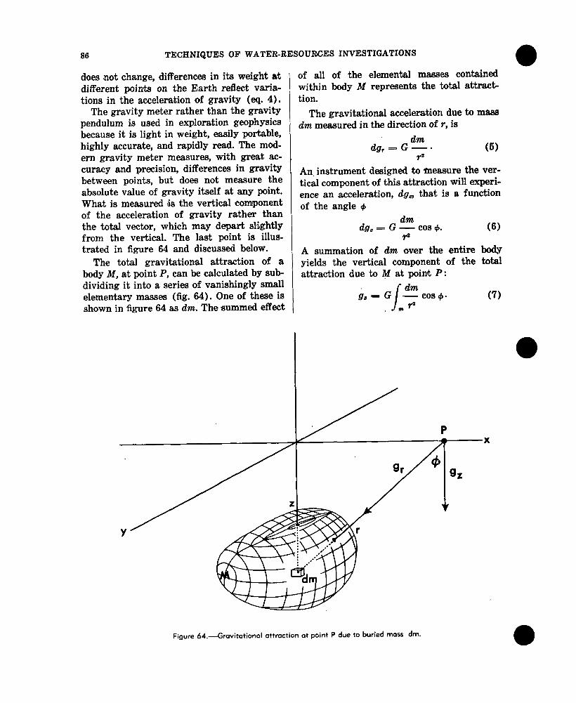
The gravity meter rather than the gravity pendulum is used in exploration geophysics becauseit is light in weight, easily portable, highly accurate, and rapidly read. The mod-ern gravity meter measures, with great ac­curacy and precision, differences in gravity between points, but does not measure the absolute value of gravity itself at any point. What is measured Is the vertical component of the acceleration of gravity rather than the total vector, which may depart slightly from the vertical. The last point is illus­trated in figure 64 and discussed below.

The total gravitational attraction of a body M, at point P, can be calculated by sub-dividing it into a series of vanishmgly small elementary masses (fig. 64). One of these is shown in figure 64 as dm. The summed effect

0 of all of the elemental masses contained within body M represents the total attracb tion.

The gravitational acceleration due to mass dm measured in the direction of r, is

dm dg, = G-- + (W

r2

An, instrument designed to measure the ver­tical component of this attraction will experi­ence an acceleration, dg, that is a function of the angle C#I

dge = G d” OS 4. ?Q

A summation of dm over the entire body yields the vertical component of the total attraction due to #I at point I’ :

gB = G (“” cos+. (7)

Figure 64.--Gravitational attraction at point P due to buried mass dm.

APPLICATION OF SURFACE GEOPHYSICS

If the density of body M is homogeneous and has the value p, we can rewrite equation 7 as :

dv gra- PG -CCh9#3 (8)

ad2Ju ’

where dv represents the volume of dm and the integration is performed over the entire volume. Equation 8 is the basic equation of gravimetry. An exact solution for the inte­gral can be obtained if the body has a simple analytical shape ; for example, a sphere, a righ,t circular cylinder, or an infinite, uni­formly thick plate. If, however, the body is irregular in shape, as most geologic bodies are, then the total attraction must be calcu­lated by graphical integration or by numeri­cal summation, using a digital or analog com,puter.

Although the gravitational attraction of any geologic body is a function of its mass, the total gravitational attraction measured by a ,gravimetric device on the surface above it ,represen,ts the sum of the attractions of both the body and the rest of the Earth, as a whole. In geophysical #prospecting, we are interested only in that part of the ,gravity field due to the body; therefore, we generally need be concerned only with the excess or deficiency of mass that the body represents, rather than with its absolute mass. Under these circumstances, the body can be de-scribed quantitatively in terms of its density contrast with its surroundings. Observed gravity variations, when corrected for non-geologic effects, refle& czmtrasts in density within the Earth, particularly, lateral con­trasts in density. The symbol p in equation 8 can be taken to represent the density con­trast between a geologic body and its sur­roundings, rather than the a&al density of

‘the body.

Reduction of Gravity Dota

Several corr&ions must be applied to raw gravity data collected in the field before they can be used for geological interpretation. Some of these corrections have a practical effeot on the design of a gravity survey and

87

the applicability of gravimetry to the hydro-geological problem at hand.

The theoretical foundations for gravity data reduction have been worked out in rigorous detail but need not be presented here. The interested reader is referred to Dobrin (1960) or Grant and West (1965) for the details and mathematical derivation of ,the cor,rections.

Reference to figure 65 should provide a qu,alitative understanding of the origin and nature of the various effects necessitating the corrections. In figure 65A is a spherical geo­logic body, the center of which lies 6.1 km (3.8 mi) below the Earth’s surface. This surface, which is perfectly flat in our exam­ple, bounds a rigid, stationary, homogeneous Earth of semi-infinite extent. The buried body, with a den&y that is 0.50 gm/cm3 greater than that of the rest of the Earth, represents the only departure from homo­geneity affecting the total gravitational field. The gravity anomaly associated with the buried sphere is shown immediately above the model. It represents a local departure from the otherwi’se featureless gravity field associated with the hypothetical Earth, and is what we would see if we were to make a series of measurements with a gravity meter in the area and plot them, without modifica­tion, on a sheet of graph paper. The maxi-mum amplitude of the anomaly is 3.7 mgals. Although spherical masses such as this one are an imprecise representation of most real geologic bodies, they are ones for which the analytical computation of gravity anomalies is relatively simple, hence in the pages that follow the sphere will be used to ill,ustrate several properties of gravity fields. Actually the Earth model we have chosen is far more unrealistic than is the sphere, insofar as a representation of nature is concerned. The real Earth is not flat, it is spheroidal, and its surface is far from plane. In addition, it is neither rigid, stationary, nor homogeneous.

A more accurate representation of the real Earth is shown in figure 65B. The Earth de­picted lthere is a rotating, nonrigid, spheroid within the gravitational influence of other

88 TECHNIQUES OF WATER-RESOUFbCES INVESTIGATIONS

5.0 I- GRAVITY ANOMALY 2 4.0 -

3.0 -

MASS EXCESS

(A)

CRUST-MANTLE

ATTRACTION DUE ERICAL MASS EXCESS

,NOT TO SCALEI (B)

Figure 65.-A, Observed gravity profile for a buried sphere in a homogeneous rigid nonrotating Earth. B, Sources of variation present in grovitotionol measure­ments made in the search for a buried sphere in a schematic, but real, Earth model.

APPLICATION OF SURFACE GEOPHYSICS 89

celestial bodies, with a compositionally homogeneous crust of geographically vary­ing thickness, and with a topographically rugged surface. Gravity measurements made on the surface of this Earth over a buried sphere would, if plotted as observed, display a scatter of points seemingly distributed without reason or order.

The reduction of gravity data refers to the removal of all unwanted effects that tend to mask or distort the gravity field causedby the object of interest. Several steps in the reduction process can be treated as mathe­matical routines, making them mechanically simple to execute. Others require judgment based on a knowledge of the local geology.

Latitude Correction Gravitational acceleration measured on the

Earth’s surface varies eve+,matically with latitude because the Earth rotates, is not perfectly rigid, and its shape is not pre­cisely that of a sphere. At the poles the dis­stance to the center of the Earth (radius RP) is less than it is at the equator (radius R,), and there is no component of centrifugal force, as there is at the equator, acting out.-ward. Both these effects tend to reduce grav­ity at the equator relative to that at the poles. The effect of a somewhat greater thickness of rock (with consequent greater mass) be-tween the equator ,and the Earth’s center tends to reduce very slightly the effect of the first two factors, but the net result is that gravity at the poles is approximately 6 gals greater than it is at the equator. This lati­tudinal variation can be expressed ;t9 a trigo­nometric function of latitude. For this reason the latitude correction is both simply and routinely determined, either from table of values at discrete increments of latitude or by high-speed machine computation.

If an accuracy of 0.1 mgal in reduced gravity data is desired, the latitude of each station must be known to within 160 meters (500 feet) of its actual location. If an ac­curacy of 0.01 mgal is needed (which is ap­proaching the limits of precision of the mod-ern field instrument), locations must be

known to within 16 meters (50 feet). With most modern topographic maps published at a scale of 1: 62,500 or larger, this is not a serious problem. The correction is made by subtracting from the value for observed gravity, the value of theoretical gravity on the reference spheroid at sea level at the same latitude. For gravity surveys of limited latitudinal extent, the vari,ation of gravity with latitude can be treated as though it were a linear function of surface distance north or south of an ~arbitrary base line drawn through the area of study. For the conti­nental United States this variation of grav­ity ranges f,rom approximately 0.6 mgal/km (0.96 mgal/mile) to 0.8 ,mgal/km (1.29 mgal/mile) and is greatest at 45” north lati-Itude.

Tidal Correction The Sun and Moon both exert an outward-

directed attraction on the gravity meter, just as they do on large bodies of water as evidenced by tides. This attraotion varies both with latitude <andtime. Although its magnitude is amall, there are some hydro-logic applications of gravimetry where tidal variations must be taken into account. The maximum amplitude of the tidal effect is approximately 0.2 mgal and its maximum rate of change is about 0.05 mgal/hour. If accuracy of this order of magnitude is not required in a gravity survey, the tidal effect may be neglected.

Several routes are open to the geophysi­cist in making tidal corrections; perhaps the one most commonly used is to monitor tidal variations, empirically, along with instru­ment drift, by returning every 2 hours or so to a gravity base station. Details of this ap­preach are discussed under the heading “Drift Correction I

Altitude Corrections Two corrections for station altitude must

be made in the data-reduction process. One of these is the free-air correction and the other is the Bouguer correction.

90 TECHNIQUES OF WATER-RESOURCES INVESTIGATIONS

Free-Air Correction

As the gravity meter is moved from hill to valley over the irregular surface of the Earth, the distance to the center of mass of the Earth varies. Equation 4 indicates that varia­tion in the value of R (the distance to the center of the Earth’s mass) will cause vari­ations in the measured ‘acceleration of grav­ity. This effect is known as the free-air effect.

The average value for the free-air gradient of gravity is -0.3086 mgal/m (-0.0941 mgal/foot). This value varies with both lab itude and altitude but the variations are very small-less than one percent over most of the Earth’s su,rface from sea level up to altitudes as great as 9,000 meters (31,000 feet). Variations in the free-air gradient of gravity also may be caused by large gravity anomalies arising from the outer part of the Earth. Departum in the measured v&e of this gradient have been fcnmd, under excep­tional circumstances, to exceed 19 percent of the average value of -0.3086 mgal/m (-0.091 mgal/foot). Knowledge of the ex-act local free-air gradient of gravity is not important in most gravity surveys. For some hydrogeologic applications, however, it may be necessary to measure the local value. Measurement of the local free-air gradient, should it be required at any locality, is not an insurmountable problem, but the neces­sity for doing so should be thoroughly evalu­ated by the geophysicist.

Bouguer Correction

The Bouguer correction is necessitated by the presence of rock between the gravity sta­tion and the elevation datum (commonly mean sea level) to which the observations are to be reduced. Referring to 65B, there is, at gravity station S,, a ,massof rock of thickness T,, between the station and the elevation datum, which cauees an additional downward attraction that would not be sensed had we been able to suspend the gravity meter in free space at the same elevation. T,his attraction varies with station

elevation and ,hasa value at station SZdiffer­tmt from that at station S1.

The standard proced,ure for making the Bouguer correction is to assume ,that an in-finite slab of rock, of thickness eNquato the height of the station above the datum, is present beneath the station. For a station in relatively flet country this approximation is a reasonable one, but for areas of rugged topography it is not. For example, in figure 65B, the infinite slab approximation is good for station S,, but poor for station S,. An adjustment is made for the relatively poor fit of the infinite slab model in topographic situations such as that of station Sz when one makes the terrain correction described below.

The gravitational acceleration due to an infinite horizontal slab of uniform density p is:

g,=2rGpT (9) where T is the thickness of the! slab. Note that the gravitational acceleration is not de-pendent on the distance of the point of meas­urement from the surface of the slab, but only on the slab’s thickness and density. Thus the gravitational acceleration caused by a given slab of homogeneous rock would be the same whether measured on its surface, or on a tower several hundred feet above its surf,ace. This apparent peculiarity of the gravitational field of an infinite slab has great utility in gravity exploration, both for data reduction and data interpretation, as will be apparent later.

Two iparameters in equation 9 are needed to make the Bouguer correction, density and thickness. In many gravity surveys, par­ticularly those of regional extent, mean sea level is chosen as the elevation datum. The value of T is then the elevation of the grav­ity station. Likewise, P routinely is assigned a constant value of 2.67 gm,/cms. These choices, though they have some theoretical and practical foundation, ,are essentially ar­bitrary and may not be appropriate for use in some areas or in certain hydrogeologic studies. When subtle gravitational variations are being sought it is important to use true

--

--

APPLICATION OF SURFACE GEOPEIYSICS

DISTANCE, IN FEET

e

18 o-

L 900 800

_- 700 L - 600 ,’

500 E - 400 f

300 z _- 200 z

DISTANCE, IN METERS

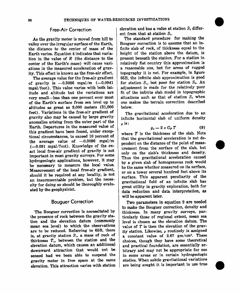
Figure 66 .-Bouguer gravity profiles across a low ridge based on six different densities employed in calculating the Bouguer correction. The proper value for density is 2.20 gm/cm’.

rock density values and to use a local eleva­tion datum.

The effect of the use of an incorrect den­sity value in making the Bouguer correction is shown in figure 66. In the lower part of figure 66 is a topographic profile of a broad ridge. This ridge is underlain by young sedi­mentary rocks that have a ,uniform density of 2.20 gm/cm3. A regional gravity gradient slopes downward ‘across the area from right to left. It is caused by a deep-seated density variation. The gravity anomaly curve labelled 2.20 is the one that would. be obtained if tidal, latitude, free-air and Bouguer correc­tions were made, using in the Bouguer cor­rection a density of 2.20 gm/cm3.

If there were no data on local rock den­siNtiesand an assumed value of 2.67 gm/cm3 were used, the reduced gravity data would provide the curve labelled 2.67. This curve, which mirrors the topography, is in error.

It displays an artificial local anomaly, su­perimposed on the regional gradient. The curve labelled “ERROR” represents the al­gebraic difference between the correct Bou­guer gravity curve, based on the true den­sity 2.20 gm/cm3, and the erroneous one created by assuming a density of 2.67 gm/ cm3.

If the density data were based on cores re-covered in an area a few miles away, where the local near-surface density was 1.60 gm/ cm3, and this value were used to make the Bouguer correction, an artificial anomaly in the form of an upward convexity superim­posed on the regional gradient (curve 1.60) is crested.

In summary, knowledge of the correct local rock density is essential to the correct reduction of gravity data. If incorrect values are used, artificial gravity anomalies related to topography are created. Hills or ridges

------------

92 TECHNIQUES OF WATERRESOURCES INVESTIGATIONS

produce artificial gravity highs if &hedensity value used is smaller than the actual value and they produce gravity lows if the density value is too hig,h.

In many regions the geology is sufficiently complex that the assu,mption of a single uniform density is not warranted. men seeking targets with very small differences in density, variable density values must be used in making the Bouguer correction. In effect, this amounts to making a correction for the near-surface geology. The more that is known about the local distribution of rock types and their densities, the less chance there ,is of introducing artificiality and error in the *result. For regional surveys of a reconnaissance nature this kind of sophisti­cation usually is not justified. For highly de-tailed studies, with closely spaced gravity stations and subtle targets, it is.

If local (rock densities are poorly known, or if the densities vary vertically, it is ad­visable to use a datum as close to the great bulk of the station elevations as possible. Either of two options can be employed. A frequency diagram of all station elevations can be plotted, and the modal elevation value for the datum selected or the elevation of the lowest station in the survey area can be used as datum Doing either minimizes the chance of errors resulting from imperfect knowledge of the geology between the station and ,the datum.

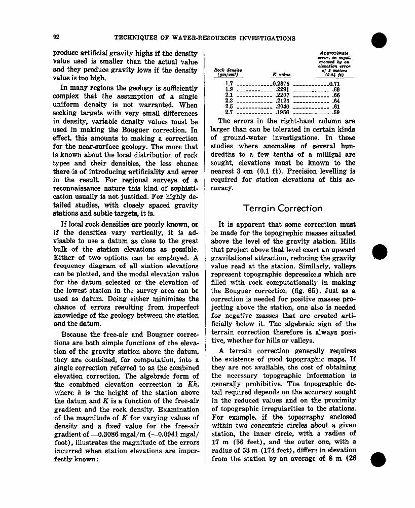
Because the free-air and Bouguer correc­tions are both simple functions of the eleva­tion of the gravity station above the datum, they are combined, for computation, into a single correction referred to as the combined elevation correction. The algebraic form of the combined elevation correction is Kh, where h is the height of the station above the datum and K is a function of the free-air grad,ient and the rock density. Examination of the magnitude of K for varying values of density and a fixed value for the free-air gradient of -0.3086 mgal/m (-0.0941 mgal/ foot), illustrates the magnitude of the errors incurred when station elevations are imper­fectly known :

l

1.7 ____________ 0.2376 ____________ 0.71 1.9 ______--____ .2291 ____________ .69 2.1 ______--__-- 2207 .66 2.3 ____________ .2123 ____________ .6i 2.6 ____________ .2040 ____________ .61 2.7 ____----____ .1966 _____m______ 59

The errors in the right-hand column are larger than can be tolerated in certain kinds of ground-water investigations. In those studies where anomalies of several hun­dredths to a few .tenths of a ,milligal are sought, elevations must be known to the nearest 3 cm (0.1 ft) . Precision levelling is required for station elevations of this ac­curacy.

Terrain Correction

It is apparent that some correction must be made for the topographic masses situated above the level of the gravity station. Hills that project above that level exert an upward gravitational attraction, reducing the gravity value read at the station. Similarly, valleys represent topographic depressions which are filled with rock computationally in making the Bouguer correction (fig. 65). Just as a correction is needed for positive masses pro­,jecting above the station, one also is needed for negative masses that are created arti­ficially below it. The algebraic sign of the terrain correction therefore is always posi­tive, whether for hills or valleys.

A terrain correction generally requires the existence of good topographic ‘maps. If they are not available, the co& of obtaining the necessary topographic information is generally prohibitive. The topographic de-tail required depends on the accuracy sought in the reduced values and on the proximity of topographic irregularities to the stations. For example, if the topography enclosed within two concentric circles about a given station, the inner circle, with a radius of 17 m (56 feet), and the outer one, with a radius of 53 m (174 feet), differs in elevation from the station by an average. of 8 m (26

APPLICATION OF SURFACE GEO,P’HYSICS 93

feet), and if the rock density is 2.67 gm/cm3, a terrain correction of approximately 0.13 mgal is required. To estimate this elevation difference accurately, a topographic map at a scale of close to 1: 25,000 or better and with a contour interval of 3-5 m (lo-15 feet) is required. In the absence of this kind of topo­graphic detail it is better not to locate the station where the terrain is varied enough to create effects of this size when high ac­culracy is sought. Balance between the detail and accuracy sought from the survey and the topographic detail available must be con­sidered in designing the survey. For a study of an intermontane valley with dimensions of 25 by 65 km (15.5 by 40.4 miles), and filled with 2,000 m (6,500 feet) of late Ceno­zoic sediments, the expectable maximum amplitude of !the associated gravity anomaly will be several tens of milligals. If one is interested only in the gross configuration of the buried abedrock floor of this valley, and in a quantitative estimate of the depth to bedrock, errors of a milligal or so can be tolerated. This means that the topographic detail needed for th,e terrain corrections is not nearly as limiting as it is for a buried outwash channel only 160 m (525 feet) deep and 1 km (0.62 mile) across. The m,aximum amplitude of the anomaly for the buried channel will not exceed 5 mgal. If the chan­nel contains clay-rich glacial till, the anomaly may be only a few tenths of a milligal. Here theaccuracyof each correction must be kept as high as possible and errors should not be allowed to exceed a few hundredths of a milligal.

Terrain corrections are made by arbitrarily subdividing the region about the ,station into a series of rectangles or curvilinear cells and estimating the average topographic elevation of each. Mathematical computations are then made to determine the correction for each cell and the results summed to obtain the total correction for the station. Either of two schemes may be used. One, a manual method, consists of centering a transparent graticule on the station, subdividing it into compart­men’ts by radii, and estimating the compart­

.

ment elevations by eye. The other, usually justified only by a relatively large number of gravity stations, consists of digitizing the topography of the surrounding region on a rectangular grid, and performing the neces­sary calculations with a high-speed digital computer. The computer program in use in the Geological Survey allows terrain correc­tion computations to be extended to a dis­tance of 166.7 km (104 miles) from the sta­tion. In most hydrologic applicatians com­putations to this distance are unnecessary. Terrain corrections are rarely extended be­yond 25 km (16 miles) when the calcula­tions are made by hand. The judgment of a person experienced in making gravity ter­rain corrections is advisable, although not absolutely necessary for efficient design of the reduction program.

Drift Correction Because the materials of construction of

most, if not all, gravity meters aYe suscepti­ble to both elastic and inelastic strains when subjected to thermal or mechanical stresses, reoccupation of the same gravity station at different times with a given meter may re-veal differences in the readings obtained. The observed differences may be caused by tidal effects, but some result from stresses or shock to the internal components of the in­strument. Gravity differences resulting from these stresses are referred to as instrument drift. In practice, instrument drift and tidal effects usually are monitored together by re­tu.rning to ,a base station every 2 hours or so during the course of a survey. It is assumed that variations between reoccupations of the base are time-dependent. Corrections for readings at field stations occupied in the interim are scaled from a plot of drift versus time.

Regional Gradients All the corrections described thus far are

designed to eliminate nongeologic effects such as those caused by variations in eleva­tion and latitude, topographic irregularities,

94 TECHNIQUES OF WATER-RESOURCES INVESTIGATIONS

or other extraneous sources. The resulting contoured gravity field is known as a com­plete Bouguer gravity anomaly map and dis­plays features that theoretically *aredue only to lateral variations in rock density below the elevation datu,m. An analysis of the grav­ity field in terms of this geology is presum­ably the reason for making the survey in the first place. From a practical standpoint, things are not quite so simple. Usually a target of geologic interest is quite specific at the outset and the gravity field arising from it is the objective sought. The problem which arises results from the fact that rarely do we seethe gravity field of a given geologic body in isolation. Usual]+, the anomaly of interest is distorted or partly masked by the gravity fields of other bodies. As a result, the geophysicist is faced with the problem of sorting out those parts of a total gravity field caused only by the object of immediate interest. Basically he knows only the mag­nitude and shape of the total Bouguer grav­ity field, but he hopes to be able to subtract from it the contributions caused by geologic bodies of unknown shape, density, and loca­tion, *in order to isolate the r&dual anomaly of interest. A simple example, ,and one for which the isolation process is usually rather simple, can be seen in figure 65B. The target here is the-spherical body. Interfering with the gravity field of the sphere is another which arises from variation in density be-tween the lower part of the crust and the mantle beneath it. The interface between the crust and mantle is not concentric with the reference spheroid and hence i#t constitutes a lateral density contrast that will be sensed by the gravity meter. Because it is a broad deep-seated feature, its gravitational effeot will be that of a gentle &really-extensive un­dulation. If the center of the anomaly sought is well up on one ilank of this undulation, the regional effect will be that of a continuous gradient extending across the survey area for a distance many times greater than the width of the target anomaly. We ‘refer to this part of the total field as the regional gradient and in order to make a quanti,tative interpre­tation of the anomaly caused by the target

alone, we must somehow subtract the effect of the regional gradient. (See fig. 71 and related text for an actual examifle of a re­gional gradient). Many schemes have been proposed for doing this. The interested reader may want to read Nettleton (1954) for a nonmathematical discussion of the methods in usetoday.

Bouguer A,nomo ly If the value of absolute gravity is known

at a station by virtue of having tied it di­rectly, or indirectly with a gravity meter, to a ‘base station where pendulu:m measure­ments of gravity have been made, the cal­culated corrections can be added algebraic-ally to this value to obtain what is known as the complete Bouguer gravity anomaly. This anomaly is defined as follows : Observed gravity plus drift and tidal correction plus combined elevation correction plus terrain correction minus theoretical gravity on the reference spheroid (latitude corm&ion).

If the terrain correotions have not been made, the results are referred to as simple Bouguer anomaly value.

In gravimetric prospecting it is not nece5 sary to know the value of absolute gravity at any point in the survey area. The concern is princi,pally with variations in Bouguer gravity from point ,to point and an arbitrary value can be assigned to the basestation. The resulting field differs from the true Bouguer anomaly field by a constant amount every-where. Knowing the value of absolute gravity at the base provides the means of tying the gravity survey to others and for this reason it is common practice to relate each survey to the same absolute datum.

Interpretation of Gravity Doto

Ambiguity In ,its simplest form, the interpretation of

gravity data consists of constructing a hypo­thetical distribution of mass that would give

APPLICATION OF SURFACE GEOPHYSICS 96

rise to a gravity field like the one observed. Models are constructed graphically or mathe­matically and their gravity-effects calculated from equation 8 by numerical summation or graphical integration. The difficulty lies in the fact that a large number (theoretically, an infinity) of hypothetical models will pro­duce the same gravity anomaly. The known quantity g. is a complex function of three

0 I 2 3 4 5 6 7 8 9 10 11 12 Miles bO- ' ' ', ' ' ', ' ' ',I ' '

= 5.0 -

unknowns: density, shape, and depth of the causative ‘body. It is apparent, even without knowledge of an exact solution for the vohrme integral in equation 8, that one could substi­tu’te, eimultaneoualy, a variety of values for the parameters ,,, r, 4, and S,dv in such a way as to maintain 8 constant value for g, at point P on the sulrface.

If we had enough information in a given

0 1 2 3 4 5 6 7 8 9 10 II 12 13 14 15 16 Milsr

0 I I I I

P“I”

IA) I I I I 0 5 IO 15 km 0 5 10 15 20 km

0 1 2 3 4 Miles 5.0 I I 1 I

Y I I 1 I I I 01234567 8 9 10 II I2 I3 14Milcr

s4.0 5.0 11

/AP=O.3 Q,,,/u I

z z t

(Cl KU 8

I I I I I 3 I I I I 9 5O I 2 3 4, 5 6 km 0 5 ID 15 20 km

Figure 67.~Schematic models and associated Bouguer gravity anomalies for idealized geologic bodies.

2

96 TECHNIQUES OF WATER-RESOURCES INVESTIGATIONS

situation to know that we were dealing with a spherical body with i’ts center buried at a spec%c depth, we still could not make a unique interpretation of the gravity anomaly in terms of size and density (fig. 67A). The gravity *anomaliesfor these four spheres are identical. This ‘results from the fact that the mass of a sphere can be treated as though it were concentrated at a (point at the center. In figure 67A, the radius and density of the spheres have ,beenadjusted to keep the total mass constant. The geologic implication is clear.

In addition, the gravity field of a sphere does not have a unique configuration (fig. 67B). Thus the shape of a body cannot be determined from its gravity anomaly alone, even when the density contrast and center of gravity are known. In figure 67B the anomaly arising from the sphere is shown as a smooth curve and the field due to an irregular body of different rotational shape, with coincident center and density, lis shown by dots. The two curves match one another very closely.

Bodies of other &ape also produce non-unique anomahes (fig. 67C). The gravityanomaly of a horizontal right circular cylinder buried at a depth slightly in excess of 3 km (1.9 miles) can be matched by that of a gently convex basement surface at a depth of approximately 1 km (0.6 mile) when the density contrast between basement and overburden matches that of the sphere and its surroundings.

In summary, the non-unliqueness is pro­nounced. The fact Chat gravimetry has been successfully employed as an exploration technique for many decades indicates that ambiguity is not an insnrmountable inter­pretation problem. For example, the indi­vidual masses and gravity fields of the spheres of different size shown in figure 67A were kept constant by holding the product pRa constant. The maximturn range of bulk densi­ties for common, naturally occurring con­solidated rocks and unconsolidated sediments is well known. Reference to Clark (1966, Sec. 4) and Manger (1963) indicates that the limits of the range ‘are approximately

1.70 land 3.00 gm/cm”. These limits represent well sorted, unconsolidated elastic sediments of hi,gh porosity and massi\.! basalt, respec­tively. T:here are a few earth materials with densities outside this range, but they are not common. This range ,placesan ulpper limit on the magnitude of the density co~dmst that one might expect to encounter in natu,re and constitutes the maximum density contrast (1.30 gm/cm3) that can be used in modelling. In most geologic settings the contrast is less than 1.00 gm/cms. Greater restriction can be placed on the density contrast in an actual setting from a knowledge of the local geology.

Other boundary conditions aan be im­posed as well. Consider a typical valley-U1 aquifer. It con&& of unconsolidated or semiconsolidated sediments resting uncom­formably on older, and usually more con­solidated (and therefore, denser), rocks. Geologic mapping determines the approxi­mate surface location of the interface be-tween the aquifer and the rocks on which it rests. If, in addition, the top of the aquifer is coincident with the surface of the ground, this fact constitutes an additional boundary condition, Further limits on the interpret% tional model can be achieved ‘by #making measurements of the average bedrock density and the density of the uppermost part of the valley fill. It can be reasonably assumed that the fill density probably increases with depth and that the walls of the valley probably slope inward in the subsurface. Thus severe hmitations have been placed upon the con­ceptual model. Several different models that will produce the observed anomaly probably can still be constructed, but the differences between the models may not be si,gnificant. If they are, ‘however, we might be able to bring other data *to bear that would furnish still further constraints and thus allow a more nearly unique interpretation. The greater the amount of geologic data that can be used in establishing ‘limits or constraints on the model, the more unique will be the interpretation.

Another facet of the interpretation process

APPLICATION OF SURFACE GEOPHYSICS 97

that is of aid in the early stages of data analysis is shown in figure 67D. Three spheres of the same size at different depths have had their densities adjusted so as to keep the maximum amplitude of their anom­alies the same. At horizontal distances that are several times the depth of burial of the spheres, all three anomalies asymptotically approach zero because the vertical compo­nent of gravity at this d,istance is negligible. Between the regions of zero and maximum ampEtude, however, the three curves are notably different. The greater the depth of burial of a given body, the gentler are the gradients of the flanks of its anomaly. The gradien~ts of any anomaly are also a function of the shape of the producing body because two bodies at disti,nctly different depths may produce anomalies with the same gradients. There ,is, however, a limit to the depth to which we can push a model and still main­tai,n anomaly gradients at or above a fixed value. For example, there is no infinitely-long, horizontal body of any cross-sectional shape that can be buried with ilts upper surface at a depth of 3 km (1.9 miles) or more and still ‘produce an anomaly that has flanking gradients as steep as those shown in figure 67D. There are some general for­mulas, based on potential theory, that allow determination of the maximum possible depth to the top of anomaly-producing body from the ratio of the maximturn amplitude to the maximum gradient of its flanks (Bott and Smith, 1958; B,ancroft, 1960). These for­mdss are useful for a rough fix on maximum depth to the top of a lbody in the early stages of modelling.

Interpretation Techniques The basic technique of gravity ‘interpreta­

tion is field matching. A model is constructed and its gravity field calculated for compari­son with the observed field.

Several methods of calculation are open to the investigator and the one chosen depends on the factors of accuracy and detail sought, the shape and complexity of the model, and the time and equipment available. All of the

methods represent ,some form of integration or summation. Computation of _the model field is followed by a comparison of the re­sults with the observed anomaly. The model is then changed and its anomaly recalculated, until the desired fit between observed and theoretical anomalies is achieved.

In its crudest form, the body under study may be assumed to have a constant density and an analytical shape (that is, a sphere, cylinder, or plate), its field being calculated by appropriate substitutions in equation 8. In its most sophisticated form the body can be given an irregular threedimensional form, with a spatially continuous or discon­tinuous distri,bution of density, and its field calculated by digital computer. The com­puter can be instructed to follow an iterative routine, wherein it makes the comparison between the observed and calculated data, institutes certain changes in the model that will lead to a better fit, recomputes the field, makes a second comparison, and eo on.

P,resentation of details of the various in­terpretation methods currently in use is rele­vant, but not appropriate here. The inter­ested reader ia referred to D&-in (1960, p. 253-262) and Grant and West (1965, p. 263-305). Two points should be stressed however; they are: (1) The solution for a given gravity anomaly is never unique and the use of highly sophisticated and elegant mathematical methods of interpretation does n:ot make it so, and (2) the quality and uniqueness of the in~terpretation are, in part, a function of the kind and amount of geologic infarmation available to the interpreter.

Significance and Use of Density Measurements

The interpretation of gravity data necessi­tates accurate knowledge of rock densities in the area surveyed. Because variations in rock density produce the potential field differ­ences we observe after data reduction, this property is of fundamental importance.

There are ,several ways in which the geo­physicist may obtain the density values to be used in handling the data for a given area.

98 TECHNIQUES OF WATER-RESOURCES INVESTIGATIONS

The cost of the method sdected should be in rough proportion to the significance of the problem. Eight methods are described briefly below. They are listed approxitmately in order of increasing significance and accuracy. 1. Assumption of a con&ant density value

of 2.67 gm/om”. 2. Assignment of density values on the basis

of lithology. Because of the wide vari­ability of rock composition and rock density within a lithologic classifica­tion, values assigned on this ,basis can be in error by ‘as much as 40 percent.

3. Estimates of densi,@ based on sound-wave velocities in rocks. Compressional wave velocities and densities of rocks are a function of some of the same lithologic factors. Because of this, they show a pronounced correlation. Approximately three-fourths of the data points in figure 68 fall within 0.1 gm/cnP of the regression curve fitted to them.

4. Iln situ gamma-gamma logging. A gamma-gamma borehole logging device meas­ures radiation that originates f’rom a source in the sonde and travels through a shell of rock adjacent to ,the borehole. The decrease in strength of the return­ing signal is approx,imately propor­tional ;to the density of the rock. How­evar, the borehole diameter, the presence of borehoe fluids, m,udcake on the hole walls, mud-filtrate invasion, and the roughness of the <holeall ad­versely affect the results. A separation of the logging tool from contact with the rock ,by as little as 0.7 cm (0.3 in) can cause a significant error in the density value.

6. Density measurementi on handspecimens collected at the outcrop. If care is taken ,to procure unweathered material, if the sampling st..ati&ics~ ‘are adequate, and if the samples are large and geologically representative, .the results of this method are ,usually quite accur,ate. This probably is the method most frequently used today.

6. Density profiling with the gravity meter. If a topographic feature such aa a hill or valley is underlain by ,rocks of laterally hohogeneous den&y and if the topography is not an expression of ,geologic structure, the data from a #gravity profile can be used to measure the average bulk density. Tlhe princi­ple is illustrated in figure 66, where the Bouguer anomaly curve computed using the correot density of 2.20 gm/ cm3 shows the least tendency to mirror the topography. The advantage of this method is that it samples, in place, a very larg& volume of rock.

7. Laboratory measurements of drillare samples of consolidated rocks. This method provides a means of sampling below &he zone of weathering and, if recovery is good, it also provides the Ibasis for computing geologically-weighted means for the secztion. Re-cent tests (McCulloh, 196G)l indicate that when proper care is #taken in handling the cores, the accuracy of this ‘method is high. However, a bore-hole represents a single vertical tra­verse of the rocks in an area. If there are pronounced lateral variations in density, cores from a single hole may not suffice.

8. Logging with a borehole gravity meter. A gravity meter lowered in a borehole can be used to measure th.e in situ density of rocks directly. Iti ability to do so stems in large part from the relationship expressed in equation 9. The difference in the acceleration of gravity between two points in a bore-hole, separated vertically ,by the dis­tance T, is a function of the product 4rrGpT. At the top of the interval downward attraction is 2rGpT and at the fbase, -2mGpT (the same attrac­tion acting upward, or in a negative sense). T can ‘be measured and the measured value of the gravity dif­ference, Ag, can be used Ito calculate the density, p. The aradius of ithe region of rock that is sampled is roughly five

APPLICATION OF SURFACE GEOPHYSICS 99

DENSITY, gm/in3 20 30 40

S-

1 5 DENSITYFgm/cm3

Figure 68.---Plot of observed compressionat wave velocities versus density for sediments and sedimentary rocks (after Grant and West, 1965). Reproduced with permission of McGraw-Hill Book Company.

100 TECHNIQUES OF WATER-RESOURCE~S INVE~STIGATIONS

times the length of the vertical inter­val, T. A typical borehole gravity meter Jog of a thick se&ion of alluvium is shown in figure 72.

Application of Gravhetry to Hydrogeology

Aquifer Geometry

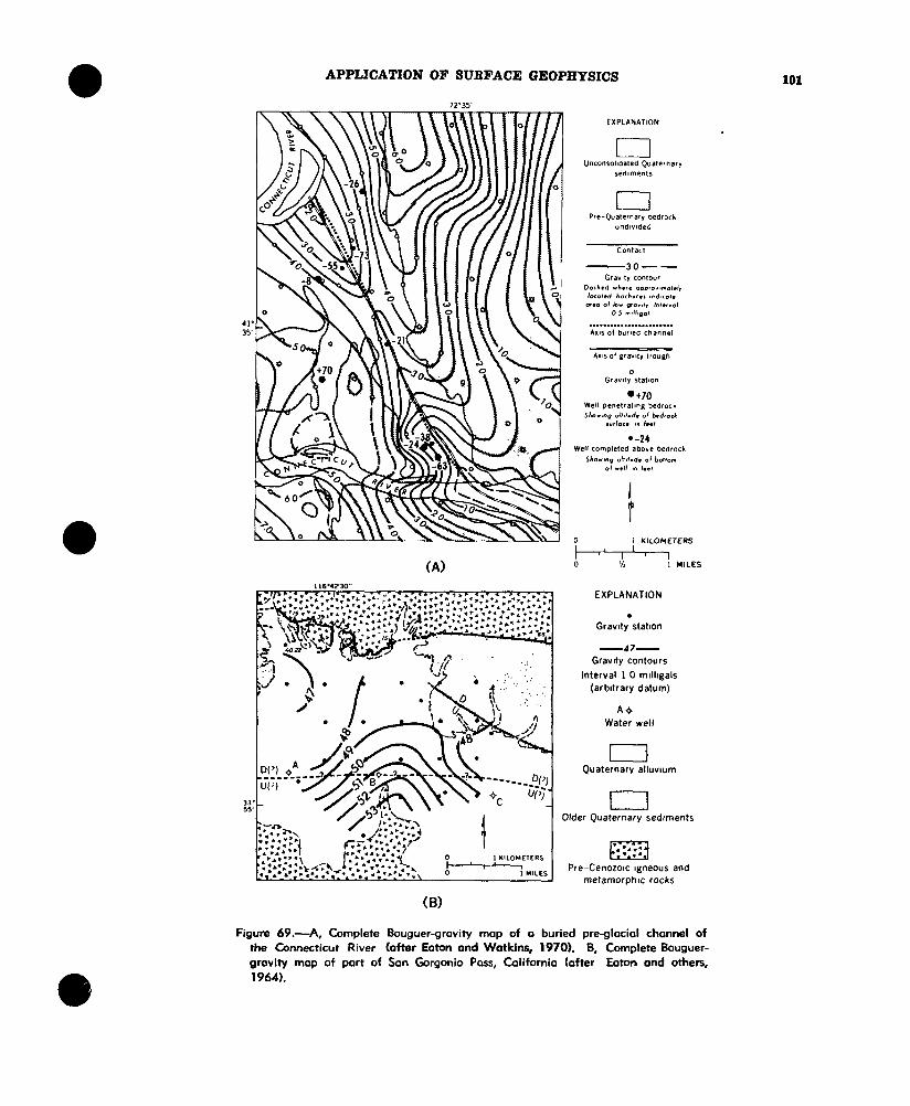
The gravity method is a rapid, inexpensive means of determining the gross configuration of an aquifer, providing an adequate density contrast between the aquifer and the under-lying ~bedrockexists. It is useful in locating areas of maximum aquifer thickness, in trac­ing the axis of a ,buried ohannd (fig. 69A), and in locating a buried ,bedrock high that may impede the flow of <groundwater (fig. 69B).

In6gure 69A, the irregular belt of unwon­solidated sediments that runs from the northwest corner of the map to the south-central part consists of buried outwash or ice-contact deposits resting in a glacially­overdeepened, preglacial bedrock channel of the Connecticut River. Well data (Cushman, 1964) defined the course of this. burled channel, and its axis coincides with the axis of the gravity trough shown. Thus the grav­ity data reflect the locus of maximum thick­nessof the unconsolidated sediments. The suc­cessof thegravity method in defining the geo­metry of the aquifer in this area is due to the high density contrast between the un­consolidated fill and the bedrock, which consists of dense Paleozoic metamorphic rocks and Triassic sedimentary rocks. In areas where the contrast is lower, the defi­nition of a narrow -buried valley, such as the one ,shown here, becomes m,ore difficult. If the density contrast is zero, the gravity method is useless for defining or mapping buried channels.

The San Gorgonio Pass area in southern California (fig. 69B) is bounded on the north and south by high m,ountain ranges consisting of Pre-Cenozoic metamorphic and

igneous rocks. These rocks have a relatively high density. Defor#med sedimentary rocks of late Tertiary age are exposed east and west of the map area along the north aide of the pass. Recent sand and gravel underlie the central part of the area. Water levels meas­ured in the spring of 1961 in two wells (A and B) define ‘8 water table sloping gently eastward with a gradient of about 5.7 m/km (30.1 feet/mile), in agreement with other well data west of the map ‘area. In the vicin­ity of well B, however, ,the water t,able drops abruptly from an elevation of 345 m (1,130 ft) to 160 m (525 ft) in well C.

Contours of complete Bouguer gravity re-veal that the cause of the discontinuity in the water table is a subsurface continuation of the exposed jbedrock ,ridge whidh projects northward from the south side of the pass. This ridge rock is virtually i,mvrmeable and serves as a ground-water barrier. Aside from its visible expression on the south side of the pass, there is no surface evidence of its presence. The gravity method thus pro­vides a means for recognizing its existence.

Estimating Average Total Porosity

Surface Method

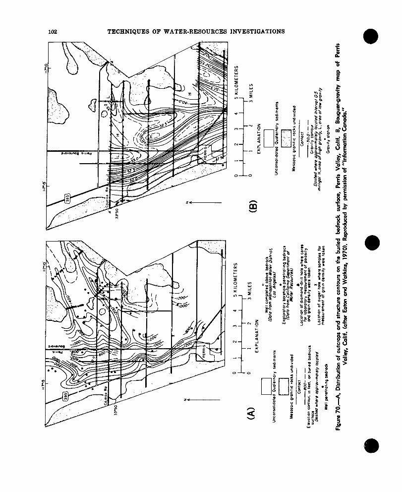
Figure 70A shows the distribution of out-crops of granitic rocks bordering Perris Valley, Calif. Also shown are structure con-tours on the lburied bedrock surface, as de-fined by well data. The structure contours reveal a large buried channel in the vicinity of Perris Boulevard. The land surf&e in this area is at an altitude of approximately 1,400 feet, which means thatthe maximum thick­ness ef the unconsolidated sediments Ming the buried valley is approximately 800 feet.

Figure 70B shows a Bouguer gravity map of the same area. The gravity map mimics the bedrock topography of the buried chan­nel ‘almost perfectly. Because of this high degree of correlation and the unusual amount of well control available f,rom the area, estimation of the average in sittu sediment porosity from surface gravity mmmrements

APPLICATION OF SURFACE GEOPEYSICS 101

EXPLANATION

-47-Gravity contours

Interval 1 0 mllhgals (arbltrary datum)

A4 Water well

1 jQuaternary alluwum

cl Older Quaternary sediments

pJ-q

Pre-Cenozoic Igneous and metamorphic rocks

(B)

Figure 69 .-A, Complete Bouguer-gravity mop of a buried pre-glociol channel of the Connecticut River (after Eaton and Watkins, 1970). B, Complete Bouguer­gravity mop of port of Son Gorgonio Pass, California (after Eaton and others, 1964).

102 TECHNIQUES OF WATER-RESOURCES INVESTIGATIONS

C h

APPLICATION OF SURFACE GEOPHYSICS 108

‘: 70- 770

2 60-T - 6.0

3 5.0 - - 50

5 4.0 - - 40

;I 30- - 3.0

>- 20- - 20I-5 LO- - 10

; o- -0

a -IO- - -10

w,-zo- - -20

g-30- - -30

g-40- - -40

y -50 - -50

W-60 - -60 -1 -_

-40-50 -60

-70

1000 m

500 m OlTl

i i i i YILES Figure 71.-Profiles of observed Bouguer gravity, residual gravity, ond calculated porosity for Perris Valley,

Calif. (after Eaton and Watkins, 1970). Reproduced by permission of “Information Canada.”

was undertaken (Eaton and Watkins, 1970). A long gravity profile was extended beyond the borders of the map at the latitude of Cajalco Bead in order to study the regional gradient. In making this profile (fig. ‘71), a different datum was employed from that on which the map was based. Hence the gravity values in figures 70B and 71 sre different. Bedrock of fairly uniform composition (granitic rock of the southern California batholith) is exposed for many miles east and west of the valley so the eastern and western branches of the observed gravity curve were used for the regional gradient, the residual anomaly due to the low density valley fill being restricted ,to the. central part of the area. If this gravity .su.rvey were part of a study of the batholith, or individual lithologic units within the batholith, it would have been necessary to define a different re­gional gradient and interpret the shape of a residual anomaly that would have included part of the regional gradient as defined here. A regional gradient is defined arbi­trarily by the objective or target, which

means that one must have at least an ap­proximate idea concerning its size and nature to begin with. All parts of the observed gravity field in figure 71 have geologic origins, but we are interested in focusing our attention only on that part arising from sources close to the surface. Hence we con­cern ourselves with that part of the curve having the steepest gradients.

The residual gravity curve was calculated by subtracting the regional gradient from the observed gxavity curve and was used, ia conj*unction with the geologic cross section shown below it, to calculate the average total porosity of the alluvial flll. Basically, the fill was weighed by the gravity meter, and, when its average #bulk demity had been determined from the gravity measurements, its porosity was calculated from the bulk density value and addi,tional measured values of average grain density. Porosity values were calculated .at six gravity stations over the central part of this valley. The results are shown in figure 71 on a porosity profile,

104 TECHNIQUES OF WATER-RESOURCES INVESTIGATIONS

where the average porosity is seen to be 33 site evaluation study and require a well or percent. For comparison, 10 samples of the borehole with a diameter of approximately fill were collected at depths ranging from 18 cm (7 in) or more in order to accept the 6 to 82 meters (20 to 270 feet) in a borehole sonde. nearby and found to have porosities ranging from 23 to 36 percent. No significance is at­tached to the convexity of the porosity profile because the resolving power of the method is not great enough to distinguish real differ­ences as small ss those shown.

Borehole Method

An in&u density log (fig. 72) of a section of u~nconsolidated sediments in Hot Creek Valley, Nev., was made using the U.S. Geo­logical Survey-LaCoste and Romberg bore-hole gravity meter system (McCulloh and others, 1967) and shows a Iremarkably sys­tematic increase in *bulk density with depth in the alluvium. At a depth of approximately 975 m (3,200 feet) the sediments have a maximum density of 2.34 gm/cm3 and remain at or near this value to a depth of 1,280 m (4,200 feet), where lake beds underlie the alluvium. ‘f’he reading interval of the gravity meter in this study was fairly coarse--61 m (200 feet) -which means that the slab of material c0ntributin.g to each calculation ex-tended horizontally away from the hole to a distance of some 300 m (935 feet). A gamma-gamma log of the same hole would have sam­pled a zone of sediments surrounding the well that was only a few centimeters thick and it could not have been used in a cased hole. If cores or cuttings had ,been taken from the well in which the density log of figure 72 was run, a highly detailed, vertical profile of porosity could have been calculated. Such a profile would ,beclearly superior to a single, averaged value of porosity as de­termined in the manner shown in 6gure 71, but the difference in co& between these two methods is considerable.

Surface gravity measurements are used primarily in a regional search and evaluation Figure 72.- In situ density log determined with a bore-study. Borehole gravity meter measurements hole grovity meter; drill hole UCe-18, Hot Creek are warranted only in the case of a detailed Valley, Nev. (after Healey, 1970).

0

------

--

APPLICATION OF SURFACEGEOPHYSICS 106 DEPTH TO WATER TABLE, IN METERS

0 20 40 60 80 100 120 140 160

-2.5 A

-3.0

m -3.5 B

s 3 g -4.0

z

=‘ -4.5 5 a 3

-5.0

-5.5

-6.0

. .

SPECIFIC RENTENTICh,, - = 0 PERCENT \ \ . \ . \

SPECIFIC RETENTION . .- \ = 20 PERCENT . . . .

MODELS \ \ .A -m B+oo .\ 0 8000 FEET LLJ2r-l

-N B,

5001 100 200 300 400 DEPTH TO WATER TABLE, IN FEET

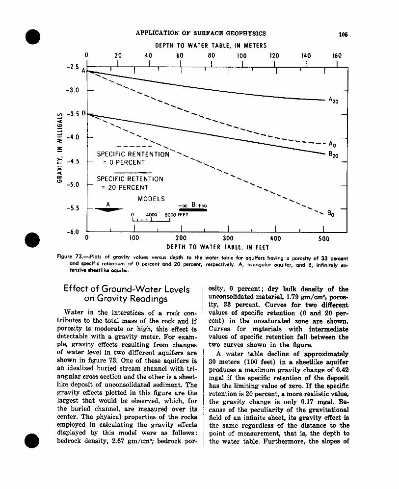
Figure 73 .-Plots of gravity values versus depth to the water table for aquifers having a porosity of 33 percent and specific retentions of 0 percent and 20 percent, tensive sheetlike aquifer.

Effect of Ground-Water Levels on Gravity Readings

Water in the interstices of a rock con-tributes to the total mass of the rock and if porosity is moderate or high, this effect is detectable with a gravity meter. For exam­ple, gravity effects resulting from changes of water level in two different aquifers are shown in figure 73. One of these aquifers is an idealized buried stream channel with tri­angular cross section and the other is a sheet-like deposit of unconsolidated sediment. The gravity effects plotted in this figure are the largest that would be observed, which, for the buried channel, are measured over its center. T’he physical properties of the rocks employed in calculating the gravi(ty effects dieplayed by this model were as follows: bedrock density, 2.67 gm/cm3; bedrock por­

respectively. A, triangular aquifer, and B, infinitely ex­

osity, 0 percent; dry bulk density of the unconsolidated material, 1.79 gm/cm*; poroc+ ity, 33 percent. Curves for two different vahies of specific retention (0 and 20 per-cent) in the unsaturated zone are shown. Curves for materials with intermediate valaes of specific retention fall between the two curves shown in the figure.

A water table decline of approximately 30 meters (106 feet) in a sheetlike aquifer produces a maximum gravity change of 0.42 mgal if the specific retention of the deposit has the limiting value of zero. If the specific retention is 20 percent, a more realistic value, the gravity change is only 0.17 mgal. Be-cause of the peculiarity of the gravit,ational field of an infinite sheet, its gravity effect is the same regardless of the distance to the point of ,measurement, that is, the depth to the water table. Furthermore, the slopes of

0

106 TECHNIQUES OF WATER-RESOURCES INVESTIGATIONS

the curves from this model are linear and are a function of the specific yield. If water-level declines in a water-table aquifer of this configuration are moni,tored with a gravity meter the aesults can (be translated into a measure of the aquifer’s specific yield. In areas of long-period water-table decline, re­peated gravity tmeaeurements, coupled with water-level observations at a few wells, would suffice for a calculation of specific yield, independent of well tests.

This use of the gravity method requires the utmost in precision and accuracy. A grav­ity difference of 0.17 mgal is a small one to measure accurately and its achievement de­pends on accuracy at every stage of the data reduction process.

References Cited Bancroft, A. M., 1960, Gravity anomalies over a

buried step: Jour. Geopbys. Research, v. 65, p. 1630-1631.

Bott, M. H. P., and Smith, R. A., 1958, The estima­tion of the limiting depth of gravitating bodies: Geophys. Prospecting, v. 6, p. l-10.

Clark, S. P., Jr., ed., 1966, Handbook of physical constants (revised edition) : Geol. Sot. America Mem. 97,587 p.

Cushman, R. V., 1964, Ground-water resources of north-central Connecticut: U.S. Geol. Survey Water-Supply Paper 1752, 96 p.

Dobrin, M. B., 1960, Introduction to geophysical prospecting: New York, N.Y., McGraw-Hill Book Co., Inc., 446 p.

Eaton, G. P., Martin, N. W., and Murphy, M. A., 1964, Application of gravity measurements to

some problems in engineering geology: Engi­neering Geology, vol. 1, no. 1, p. 621.

Eaton, G. P., and Watkins, J. S., 1970, The use of seismic refraction and gravity methods in hy­drogeological investigations : Proc. Canadian Centennial Conf. Mining and Ground-Water Geophysics, Ottawa.

Grant, F. S., and West, G. F., 1965, Interpretation theory in applied geophysics: New York, N.Y., McGraw-Hill Book Co., Inc., 583 p.

Healey, D. L., 1970, Calculated in situ bulk den­sities from subsurface gravity observations and density logs, Nevada Test Site and Hot Creek Valley, Nye County, Nevada.: U.S. Geol. Survey Prof. Paper 700-B, p. 52-62.

Manger, G. E., 1963, Porosity and bulk density of sedimentary rocks: U.S. Geol. Survey Bull. 1144-E, 55 p.

McCulloh, T. H., 1965, A confirmation by gravity measurements of an underground density pro-file based on core densities: Geophysics, v. 30, p. 1108-1132.

McCulloh, T. H., LaCoste, L. J. B., Schoellhamer, J. E., and Pampeyan, E. H., 1967, The U.S. Geological Survey-La&& and Romberg pre­cise borehole gravimeter system--Instrumen­tation and support equipment, i:n Geological Survey Research 1967: U.S. Geol. Survey Prof. Paper 575-D, p. D92-DlOO.

Nettleton, L. L., 1954, Regionals, residuals and structures: Geophysics, v. 19, p. l-22.

Schwennesen, A. T., 1917, Ground water in San Simon Valley, Arizona and New Mexico, in Contributions to the Hydrology of the United States, 1917: U.S. Geol. Survey Water-Supply Paper 425, p. l-35.

White, N. D., 1963, Analysis and evaluation of available hydrologic data for San Simon Basin, Cochise and Graham Counties, Arizona: U.S. Geol. Survey Water-Supply Paper 1619-DD, p. DDl-DD33.