application of the symplectic finite-difference time-domain method to light scattering by small...

Application of the symplectic finite-differencetime-domain method to light scattering by smallparticles

Peng-Wang Zhai, George W. Kattawar, Ping Yang, and Changhui Li

A three-dimensional fourth-order finite-difference time-domain (FDTD) program with a symplectic in-tegrator scheme has been developed to solve the problem of light scattering by small particles. Thesymplectic scheme is nondissipative and requires no more storage than the conventional second-orderFDTD scheme. The total-field and scattered-field technique is generalized to provide the incident wavesource conditions in the symplectic FDTD (SFDTD) scheme. The perfectly matched layer absorbingboundary condition is employed to truncate the computational domain. Numerical examples demonstratethat the fourth-order SFDTD scheme substantially improves the precision of the near-field calculation.The major shortcoming of the fourth-order SFDTD scheme is that it requires more computer CPU timethan a conventional second-order FDTD scheme if the same grid size is used. Thus, to make the SFDTDmethod efficient for practical applications, one needs to parallelize the corresponding computationalcode. © 2005 Optical Society of America

OCIS codes: 010.1290, 010.1310, 010.3920, 290.1090, 290.5850, 280.1310.

1. Introduction

The conventional implementation of the finite-difference time-domain method (FDTD),1–4 which isbased on the second-order differencing operation inboth space and time, has been used extensively to solvevarious electromagnetic scattering problems,5–10 how-ever, for an increasing number of applications thisalgorithm has insufficient accuracy11 and demandsvast computational resources. In our experience withFDTD computations, the numerical errors are nor-mally acceptable for computing the phase function,but the errors for the other phase matrix elementsare generally much larger. To reduce the errors inthese matrix elements, we must use a quite smallspatial grid size leading to substantial memory re-quirements. A fine grid resolution is usually imprac-tical in terms of the demand on computationalresources in many situations. One natural solution isto use schemes with higher-order accuracy without

increasing their demand on computer memory. A fewhigher-order schemes have been proposed.12–15 Oneapproach needs to manage the second-order spacederivatives of the permeability or permittivity, whichis quite complicated if the permittivity or permeabil-ity varies in space.12,13 Another approach uses theRunge–Kutta method, which is dissipative and de-mands more storage of data for the intermediatestages.15

Symplectic integrators are numerical integrationschemes for Hamiltonian systems16–18 and have beenintroduced to the FDTD technique19,20; however, rig-orous application of the symplectic integrator tothree-dimensional problems is rather complicated be-cause of the complication of discretization of theHamiltonian of the electromagnetic field in a three-dimensional case. Hence direct application of thesymplectic integrator scheme to Maxwell’s equationshas been made by Hirono21 to obtain a concise fourth-order symplectic FDTD (SFDTD) solver. The fourth-order SFDTD scheme is nondissipative and requiresno more storage than the traditional second-orderFDTD scheme.21 In this study we generalize thesecond-order total-field and scattered-field (TF–SF)source condition technique2,22,23 to SFDTD, thereforemaking the SFDTD scheme suitable for solution oflight-scattering problems.

The current version of our SFDTD code calculatesjust the near fields for the problem of light scattering

All the authors are with Texas A&M University, College Station,Texas 77843. P.-W. Zhai ([email protected]), G. W. Kattawar([email protected]), and C. Li ([email protected]) are with the De-partment of Physics; P. Yang ([email protected]) is withthe Department of Atmospheric Sciences.

Received 31 August 2004; accepted 3 November 2004.0003-6935/05/091650-07$15.00/0© 2005 Optical Society of America

1650 APPLIED OPTICS � Vol. 44, No. 9 � 20 March 2005

by an arbitrary particle. To obtain the complete phasematrix that represents far-field behavior, a second-order near-to-far-field transformation7,24 should begeneralized to its fourth-order counterpart. This ef-fort is currently ongoing. The truncation of the com-putational domain is made by the perfectly matchedlayer (PML) absorbing boundary condition25 withfourth-order accuracy in time and space.26 In Section2 we present the theoretical framework for theSFDTD scheme related to scattering problems, andin Section 3 we demonstrate the performance of theSFDTD scheme by numerical calculations. Finally,conclusions are given in Section 4.

2. Theoretical Formulas for the SymplecticFinite-Difference Time-Domain Scheme

A. Basic Formulation

The three-dimensional SFDTD scheme was proposedby Hirono et al.21,26 The basic formulas developedspecifically to solve scattering problems are brieflypresented here for completeness. Maxwell’s equa-tions in an isotropic, sourceless dielectric medium canbe written in matrix form as follows:

�

�t �HE�� W�HE�, (1a)

W � U � V, (1b)

U � �(0) �cR(0) (0) �, (1c)

V � � (0) (0)cR��r � � · I3

�, (1d)

where H � �Hx, Hy, Hz�T and E � �Ex, Ey, Ez�T are theelectromagnetic field matrices, where superscript Trepresents the transpose matrix; c is the speed oflight in vacuum; (0) is the 3 � 3 null matrix; �� kc�i��r�, I3 is the 3 � 3 unit matrix; �r � i�i is thecomplex permittivity; and R is the 3 � 3 matrix rep-resenting the curl operator

R �

0 �

�

�z�

�y�

�z0 �

�

�x

��

�y�

�x0

. (1e)

According to the symplectic integrator propagatortheory, the solution of Eqs. (1a)–(1e) after time step �t

can be expressed by

�HE�(�t) � exp(�tW)�HE�. (2)

If U and V do not commute, the exponential propa-gator can be approximated by

exp(�tW) � IIp�1

mexp(dp�tV)exp(cp�tU) � O[(�t)

n�1],

(3)

where n is the order of the approximation, m is thestage number of the propagator, and cp and dp arereal coefficients that characterize the propagator.The values of the coefficients for second-order andfourth-order approximations are listed in Table1.15–18

Since U2 � �0�,

exp(�tU) � I6 � �tU, (4)

where I6 is the 6 � 6 unit matrix. We can calculateexp��tV� as follows:

exp(�tV) � �n�0

(�tV)n�n !

�� I3 (0)1 � exp(��t)

�cR��r exp(��t) · I3�.

(5)

Using the coefficients cp and dp of order n and choos-ing an approximation of order h for the first-orderpartial differential operators in R, Eqs. (2) and (3)give a FDTD scheme of nth order in time and hthorder in space. Here we choose the fourth-orderscheme in both time and space based on the equa-tions. The Yee lattice1,8 is used to discretize the com-putational domain. The fourth-order approximationfor the first-order space differential operators is asfollows:

��f�x�i

27(fi�1�2 � fi�1�2) � fi�3�2 � fi�3�2

24�x . (6)

Applying exp�cp�tU� to �Hn��p�1��5, En��p�1��5�T, we canobtain Hn�p�5. For example, the detailed expression ofthe y component of the magnetic field at the pth stageis as follows:

Table 1. Coefficients of the Symplectic Integrator Propagatorscp � cm�1�p�0 p m � 1�, dp � dm�p�0 p m�, dm � 0

CoefficientsSecond OrderSecond Stage Fourth Order Fifth Stage

c1 0.5 0.17399689146541d1 1.0 0.62337932451322c2 0.5 �0.12038504121430d2 0.0 �0.12337932451322c3 — 0.89277629949778d3 — �0.12337932451322

20 March 2005 � Vol. 44, No. 9 � APPLIED OPTICS 1651

Hyn�p�5�i, j �

12, k�� Hy

n�(p�1)�5�i, j �12, k�

�c�tcp

�z 98 �Ex

n�(p�1)�5�i, j

�12, k �

12�

� Exn�(p�1)�5�i, j �

12, k �

12��

�124 �Ex

n�(p�1)�5�i, j �12, k �

32�

� Exn�(p�1)�5�i, j �

12, k �

32��

�c�tcp

�x 98 �Ez

n�(p�1)�5�i �12, j

�12, k�

� Ezn�(p�1)�5�i �

12, j �

12, k��

�1

24 �Ezn�(p�1)�5�i �

32, j �

12, k�

� Ezn�(p�1)�5�i �

32, j �

12, k��,

(7)

where n is the standard notation for time steps and pdenotes the stage of the field vectors. Similarly, byapplying exp�dp�tV� to �Hn��p�1��5, En��p�1��5�T, we ob-tain the electric field at the next stage. For example,the x component of the electric field at the pth stageis as follows:

where �r is the local real permittivity at point �i, j� 1�2, k � 1�2� in this paper. Sun and Fu9 discussedthe effects of different averaging schemes for thepermittivity for the FDTD method. They concludedthat the local value of the permittivity should beused in the FDTD method. To compare with the bestperformance of the FDTD method, we also adoptedthe local value of permittivity in the SFDTDmethod.

B. Total-Field and Scattered-Field Source ConditionUsed in the Scattering Problem

Given Eqs. (7) and (8) and the equations of other fieldvectors, we can generalize the TF–SF plane wavesource condition2,22,23 to the symplectic scheme. Theinterface surface of the TF–SF regions in the Yee

space lattice is composed of six flat planes that forma rectangular box, as shown in Fig. 1(a). Suppose theTF–SF interface is located in a source-free vacuum.In the following discussion we give the consistencyconditions for Ex around region b in Fig. 1(a). Figure1(b) shows in detail the top view of the Yee structurein region b, where the arrows represent Ex, the circlesrepresent Hz, and the solid line is the TF–SF inter-face. At the left of the solid line is the SF region, at the

Exn�p�5�i, j �

12, k �

12�� exp(��dp�t)Ex

n�(p�1)�5�i, j �12, k �

12�

�1 � exp(��dp�t)

��r�y c98 �Hz

n�p�5�i, j � 1, k �12�� Hz

n�p�5�i, j, k �12��

124 �Hz

n�p�5�i, j � 2, k �12�

� Hzn�p�5�i, j � 1, k �

12��

1 � exp(��dp�t)��r�z c9

8 �Hyn�p�5�i, j �

12, k � 1�

� Hyn�p�5�i, j �

12, k��

124 �Hy

n�p�5�i, j �12, k � 2�� Hy

n�p�5�i, j �12, k � 1��, (8)

Fig. 1. (a) Six-sided TF–SF interface surface for the three-dimensional symplectic FDTD space lattice. (b) A detailed top viewof the Yee structure in region b, where the arrows represent Ex, thecircles represent Hz, and the solid line represents the TF–SF in-terface. At the left of the solid line is the SF region and at the rightof that line is the TF region.


right of that line is the TF region. From Eq. (8) theconsistency condition for Ex in region b is

where Hi, zn�p�5 is the z component of the incident

magnetic field. In Eqs. (9a)–(9c), i ranges from i0 to i1,whereas k ranges from k0 � 1�2 to k1 � 1�2. Theconsistency condition for other field vectors at otherlocations can be obtained in a similar manner.

The generation of a look-up table for Hi and Ei

around the TF–SF interface is similar to the second-order case; however, here we should use the fourth-order one-dimensional plane wave that we obtainedby setting Ez � 0 in Eq. (7) and Hz � 0 in Eq. (8).Four-point polynomial interpolation is used for inter-polation of look-up-table data. The time-dependentsource wave located at grid point ks is

Exn�p�5(ks) � g[n�(p)�t], (10)

where g is an arbitrary time function: n��p� � n� �l�1

p cl.

C. Perfectly Matched Layer Absorbing BoundaryCondition

The traditional PML absorbing boundary condition25

has been extended to a fourth-order symplecticscheme.26 By defining H� � �Hxy, Hxz, Hyz, Hyx,Hzx, Hzy�T and E� � �Exy, Exz, Eyz, Eyx, Ezx, Ezy�T, we canthen write the equations for H� and E� in matrixform:

�

�t �H�

E�� W��H�

E��, (11a)

W� � �� R�

R� ��, (11b)

where �= is a matrix defined as follows:

�11� � �66� �4��y

c , (11c)

�22� � �33� �4��z

c , (11d)

�44� � �55� �4��x

c , (11e)

�ij� � 0, i j, (11f)

where �x, �y, and �z are the conductivities in the PMLregion; and R� is the matrix defined as

R15� � R16� � �R61� � �R62� ��

�y, (11g)

R31� � R32� � �R23� � �R24� ��

�z, (11h)

R53� � R54� � �R45� � �R46� ��

�x, (11i)

Rij� � 0 (11j)

for all other elements.We then write

W� � �� R�

(0) (0) �� (0) (0)R� �� (12)

and apply the symplectic integrator propagator algo-rithm to Eqs. (11a)–(11j) to determine the PML ab-sorbing boundary condition for the SFDTD method.For example,

Hxyn�p�5(i � 1�2, j, k)

� exp(��y�c�tcp)Hxyn�(p�1)�5(i � 1�2, j, k)

�1 � exp(��y�c�tcp)

�y�

�Ezn�(p�1)�5

�y (i � 1�2, j, k),

(13)

where �y� � 4��y�c, and �y is the conductivity at point�i � 1�2, j, k� in the PML region; �Ez

n��p�1��5�i� 1�2, j, k��y is determined by approximation (6).

Exn�p�5(i, j0 � 1�2, k � 1�2) � Ex

n�p�5(i, j0 � 1�2, k � 1�2) �c�tdp

24�y Hi, zn�p�5(i, j0 � 1, k � 1�2), (9a)

Exn�p�5(i, j0 � 1�2, k � 1�2) � Ex

n�p�5(i, j0 � 1�2, k � 1�2) �c�tdp

�y

� �98 Hi, z

n�p�5(i, j0 � 1, k � 1�2) �1

24 Hi, zn�p�5(i, j0 � 2, k � 1�2)�, (9b)

Exn�p�5(i, j0 � 3�2, k � 1�2) � Ex

n�p�5(i, j0 � 3�2, k � 1�2) �c�tdp

24�y Hi, zn�p�5(i, j0, k � 1�2), (9c)


3. Numerical Results and Discussion

Based on the theoretical discussion in Section 2, wehave developed a three-dimensional SFDTD code cal-culating the near field for the problems of light scat-tering by arbitrary particles. For the numericalexamples shown in this paper, we used an eight-layerPML with reflection coefficient R�0� � 10�12. The freespace between the particle and the PML absorbingboundary condition is seven layers. As we noted inSection 2, the permittivities at the boundary of theparticle are set to be the local values. The effects ofthe different averaging methods for the permittivitiesare possible areas of future study for the SFDTDmethod.

The first case we studied is the problem of a one-dimensional electromagnetic wave that propagatesthrough free space. The source for this study is givenby

Exn(ks � 1�2) � exp[�(n�ndecay � n0)

2], (14)

where ks � 1, ndecay � 10, and n0 � 5. For the simu-lation we used �z � ��20 and c�t��z � 0.5, where cis the speed of light in vacuum and �t and �z are thegrid size in time and space, respectively. Figure 2shows a comparison of the snapshots of the Ex distri-bution along the z axis in the time domain calculatedby the analytical theory and the FDTD and SFDTDmethods. At n � 250, the SFDTD method is in goodagreement with the theory, whereas the profile cal-culated by the FDTD method is slightly distortedfrom that of the theory. At n � 1000, the profile

calculated by the SFDTD scheme still complies withthe theory, whereas the profile of the FDTD schemehas developed into several peaks because of numeri-cal dispersion. Figure 2 clearly demonstrates that theSFDTD method has smaller numerical dispersioncompared with the FDTD method.

Figure 3 shows the validity of the symplecticfourth-order TF–SF source condition. Consider apulsed plane wave such as in Eq. (14) propagatingthrough free space along the z direction. According tothe TF–SF technique, we should see a pulsed planewave such as that in Fig. 1 propagating inside theTF–SF surface while the fields outside the TF–SF

Fig. 2. Snapshots of the Ex field distribution in a one-dimensionalgrid in a time domain calculated by Mie theory and FDTD andSFDTD methods. c�t��z � 0.5 and free space are assumed. (a)n � 250 and (b) n � 1000.

Fig. 3. TF–SF grid zoning for a pulsed plane wave propagating infree space. The three snapshots calculated by the SFDTD schemeshow the Ex field distribution at the x–z plane at three time steps.


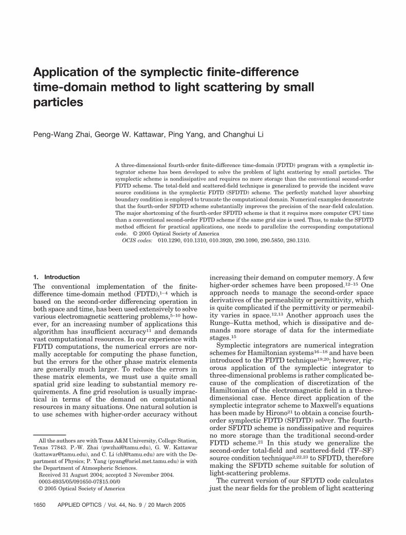
surface are zero. Figure 3 shows snapshots of the Ex

field distribution at three instants in the x�z plane,where (a) is for n � 60, (b) is for n � 90, and (c) is forn � 120. The incident wave is chosen to be a Gauss-ian pulse with ndelay � 30 and n0 � 5. In three-dimensional space, �1 � ��20 and c�t��1 � 0.99��3,where �1 is the grid size for all three dimensions. Theone-dimensional incident wave has c�t��2 � 0.5,where �2 is the grid size for the one-dimensionalspace. The TF zone spans 48 � 48 � 48 cells and issurrounded on each side by a 12�cell SF zone. At n� 60, the wave just gets into the TF region and onlyhalf of the wave packet appears; at n � 90, the wavepropagates to the center of the TF region; at n� 120, the front half of the profile has already goneout of the TF region. Meanwhile, the largest fieldvalues in the scattering zone are of the order of mag-nitude of 10�6.

It is straightforward to apply the SFDTD scheme toscattering problems with the symplectic fourth-orderTF–SF source condition. Now consider an x-polarizedincident wave that propagates along the z directionand is then scattered by a spherical dielectric parti-cle. The center of the spherical particle is chosen asthe origin of the coordinate system. The size param-eter is 10 and the refractive index is 1.0925� i0.248, which is the refractive index for ice crystalsat 11��m wavelength. The grid sizes and time stepsare set the same as in Fig. 3. Define A � |Ex| as theamplitude of Ex in the frequency domain and �� arg�Ex� is the phase of Ex. The relative error of Acalculated by the FDTD or the SFDTD method rela-tive to the Mie solution is defined as � � �A� AMie��AMie � 100%; phase error �� is defined as�� Mie, where AMie and �Mie are calculatedfrom Mie theory.

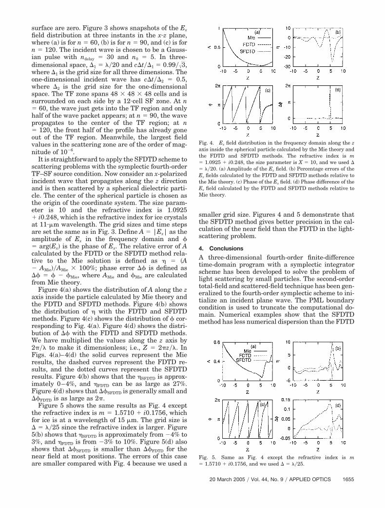
Figure 4(a) shows the distribution of A along the zaxis inside the particle calculated by Mie theory andthe FDTD and SFDTD methods. Figure 4(b) showsthe distribution of � with the FDTD and SFDTDmethods. Figure 4(c) shows the distribution of � cor-responding to Fig. 4(a). Figure 4(d) shows the distri-bution of �� with the FDTD and SFDTD methods.We have multiplied the values along the z axis by2�� to make it dimensionless; i.e., Z � 2�z��. InFigs. 4(a)–4(d) the solid curves represent the Mieresults, the dashed curves represent the FDTD re-sults, and the dotted curves represent the SFDTDresults. Figure 4(b) shows that the �SFDTD is approx-imately 0–4%, and �FDTD can be as large as 27%.Figure 4(d) shows that ��SFDTD is generally small and��FDTD is as large as 2�.

Figure 5 shows the same results as Fig. 4 exceptthe refractive index is m � 1.5710 � i0.1756, whichfor ice is at a wavelength of 15 �m. The grid size is� � ��25 since the refractive index is larger. Figure5(b) shows that �SFDTD is approximately from �4% to3%, and �FDTD is from �3% to 10%. Figure 5(d) alsoshows that ��SFDTD is smaller than ��FDTD for thenear field at most positions. The errors of this caseare smaller compared with Fig. 4 because we used a

smaller grid size. Figures 4 and 5 demonstrate thatthe SFDTD method gives better precision in the cal-culation of the near field than the FDTD in the light-scattering problem.

4. Conclusions

A three-dimensional fourth-order finite-differencetime-domain program with a symplectic integratorscheme has been developed to solve the problem oflight scattering by small particles. The second-ordertotal-field and scattered-field technique has been gen-eralized to the fourth-order symplectic scheme to ini-tialize an incident plane wave. The PML boundarycondition is used to truncate the computational do-main. Numerical examples show that the SFDTDmethod has less numerical dispersion than the FDTD

Fig. 4. Ex field distribution in the frequency domain along the zaxis inside the spherical particle calculated by the Mie theory andthe FDTD and SFDTD methods. The refractive index is m� 1.0925 � i0.248, the size parameter is X � 10, and we used �

� ��20. (a) Amplitude of the Ex field. (b) Percentage errors of theEx fields calculated by the FDTD and SFDTD methods relative tothe Mie theory. (c) Phase of the Ex field. (d) Phase difference of theEx field calculated by the FDTD and SFDTD methods relative toMie theory.

Fig. 5. Same as Fig. 4 except the refractive index is m� 1.5710 � i0.1756, and we used � � ��25.


method. The validity of the generalized TF–SF tech-nique has been shown. For the problems of light scat-tering by spherical dielectric particles, we calculatedthe near fields by Mie theory and the FDTD andSFDTD methods. The results show that the SFDTDmethod gives more accurate results in the computa-tion of the near field than the FDTD method. For thereaders who are interested in more detailed informa-tion about the Courant–Friedrichs–Levy conditionand computation resources requirement for theSFDTD method, please refer to Ref. 21.

This study was partially supported by the U.S. Of-fice of Naval Research under contract N00014-02-1-0478 and by the Center for Atmospheric Chemistryand the Environment (G. W. Kattwar) and was alsosupported by a National Science Foundation (NSF)CAREER Award research grant ATM-0239605 fromthe NSF Physical Meteorology Program and NASAresearch grants NAG-1-02002 and NAG5-11374 fromthe NASA Radiation Science Program managed byDonald Anderson and Hal Maring.

References1. K. S. Yee, “Numerical solution of initial boundary value prob-

lems involving Maxwell’s equations in isotropic media,” IEEETrans. Antennas Propag. AP-14, 302–307 (1966).

2. K. R. Umashankar and A. Taflove, “A novel method to analyzeelectromagnetic scattering of complex objects,” IEEE Trans.Electromagn. Compat. EC-24, 397–405 (1982).

3. A. Taflove and S. C. Hagness, Computational Electromagnet-ics: the Finite-Difference Time-Domain Method, 2nd ed. (Ar-tech House, Norwood, Mass., 2000).

4. K. S. Kunz and R. J. Luebbers, The Finite Difference TimeDomain Method for Electromagnetics (CRC Press, Boca Raton,Fla., 1993).

5. P. Yang and K. N. Liou, “Light scattering by hexagonal icecrystals: comparison of finite-difference time domain and geo-metric optics models,” J. Opt. Soc. Am. A 12, 162–176 (1995).

6. P. Yang and K. N. Liou, “Finite-difference time domain methodfor light scattering by small ice crystals in three-dimensionalspace,” J. Opt. Soc. Am. A 13, 2072–2085 (1996).

7. W. Sun, Q. Fu, and Z. Chen, “Finite-difference time-domainsolution of light scattering by dielectric particles with a per-fectly matched layer absorbing boundary condition,” Appl. Opt.38, 3141–3151 (1999).

8. P. Yang and K. N. Liou, “Finite-difference time-domainmethod for light scattering by nonspherical and inhomoge-neous particles,” in Light Scattering by Nonspherical Particles:Theory, Measurements, and Applications, M. I. Mishchenko,S. W. Hovenier, and L. D. Travis, eds. (Academic, San Diego,Calif., 2000), pp. 173–221.

9. W. Sun and Q. Fu, “Finite-difference time-domain solution oflight scattering by dielectric particles with large complex re-fractive indices,” Appl. Opt. 39, 5569–5578 (2000).

10. S. C. Hill, G. Videen, W. Sun, and Q. Fu, “Scattering andinternal fields of a microsphere that contains a saturable ab-

sorber: finite-difference time-domain simulations,” Appl. Opt.40, 5487–5494 (2001).

11. K. L. Shlager and J. B. Schneider, “Comparison of the disper-sion properties of several low-dispersion finite-difference time-domain algorithms,” IEEE Trans. Antennas Propag. 51, 642–653 (2003).

12. J. Fang, “Time domain finite difference computation for Max-well’s equations,” Ph.D. dissertation (Department of ElectricalEngineering, University of California at Berkeley, Berkeley,Calif., 1989).

13. T. Deveze, L. Beaulieu, and W. Tabbara, “A fourth orderscheme for the FDTD algorithm applied to Maxwell’s equa-tions,” in Proceedings of the 1992 International IEEE Antennasand Propagation Society Symposium (Institute of Electricaland Electronics Engineers, Piscataway, N.J., 1992), pp. 346–349.

14. C. W. Manry, S. L. Broschat, and J. B. Schneider, “Higher-order FDTD methods for large problems,” Appl. Comput. Elec-tromagn. Soc. J. 10, 17–29 (1995).

15. J. L. Young, D. Gaitonde, and J. S. Shang, “Toward the con-struction of a fourth-order difference scheme for transient EMwave simulation: staggered grid approach,” IEEE Trans. An-tennas Propag. 45, 1573–1580 (1997).

16. M. Suzuki, “Fractal decomposition of exponential operatorswith applications to many-body theories and Monte Carlo sim-ulation,” Phys. Lett. A 146, 319–323 (1990).

17. H. Yoshida, “Construction of higher order symplectic integra-tors,” Phys. Lett. A 150, 262–268 (1990).

18. M. Suzuki, “General theory of fractal path integrals with ap-plications to many-body theories and statistical physics,” J.Math. Phys. Lett. 32, 400–407 (1991).

19. T. Hirono, W. W. Lui, and K. Yokoyama, “Time-domain simu-lation of electromagnetic field using a symplectic integrator,”IEEE Microwave Guid. Wave Lett. 7, 279–281 (1997).

20. I. Saitoh, Y. Suzuki, and N. Takahashi, “The symplectic finitedifference time domain method,” IEEE Trans. Magn. 37,3251–3254 (2001).

21. T. Hirono, W. Lui, S. Seki, and Y. Yoshikuni, “A three-dimensional fourth-order finite-difference time-domainscheme using a symplectic integrator propagator,” IEEETrans. Microwave Theory Tech. 49, 1640–1648 (2001).

22. G. Mur, “Absorbing boundary conditions for the finite-difference approximation of the time-domain electromagneticfield equations,” IEEE Trans. Electromagn. Compat. EC-23,377–382 (1981).

23. Ref. 3, pp. 175–233.24. P.-W. Zhai, Y.-K. Lee, G. W. Kattawar, and P. Yang, “Imple-

menting the near- to far-field transformation in the finite-difference time-domain method,” Appl. Opt. 43, 3738–3746(2004).

25. J.-P. Berenger, “A perfectly matched layer for the absorption ofelectromagnetic waves,” J. Comput. Phys. 114, 185–200(1994).

26. T. Hirono, W. W. Lui, and S. Seki, “Successful applications ofPML-ABC to the symplectic FDTD scheme with 4th-order ac-curacy in time and space,” in Vol. 3 of Microwave SymposiumDigest, 1999 IEEE MTT-S International (Institute of Electricaland Electronics Engineers, Piscataway, N.J., 1999), pp. 1293–1296.


application of the symplectic finite-difference time-domain method to light scattering by small...

Documents