115

AMO – Advanced Modeling and Optimization, Volume 11, Number 2, 2009

Application of Variance Based Sensitivity Analysis to

Blade Outer Air Seals

S. Finley1*, V. Sidwell2, P. Marzocca1, K. Willmert1

1 Clarkson University, Mechanical & Aeronautical Engineering Department, 8 Clarkson Ave, Potsdam, NY, 13699

2Pratt & Whitney, 400 Main St., East Hartford, CT 06108 * Corresponding Author, Phone: 607-759-0141,e-mail: finleysj@clarkson.edu

Abstract

Process improvement is an important method to sustain competitive improvement. To achieve

process improvement, a company may require custom software that is specific to their needs. However,

developing custom standalone software packages is complex and often out of a company’s area of

expertise. Modifying commercial software is more cost effective for a company. This paper examines the

new capabilities that become available when commercial Computer Aided Design, Finite Element

Analysis, and Optimization software are integrated together for Multi-Disciplinary Optimization.

Specifically, sensitivity analyses and an optimization are conducted to answer manufacturing and design

questions. Engineers will know how to reduce variation in the manufacturing process and how to design an

improved product. Without the custom software, it would be infeasible to conduct a sensitivity analysis or

an optimization. Thus, the development of the modified commercial software can lead to a technological

competitive advantage.

AMO – Advanced Modeling and Optimization. ISSN: 1841-4311

116

List of Acronyms

APDL ANSYS® Parametric design Language API Application Program Interface BOAS Blade Outer Aid Seal CAD Computer Aided Design CAE Computer Aided Engineering CAM Computer Aided Manufacturing CAPP Computer Aided Process Planning CFD Computational Fluid Dynamics CTCD Centre for Terrestrial Carbon Dynamics FEA Finite Element Analysis GA Genetic Algorithm GEM-SA Gaussian Emulation Machine for Sensitivity Analysis GUI Graphical User Interface LCF Low Cycle Fatigue LSGRG Large Scale Generalized Reduced Gradient MDO Multi-Disciplinary Optimization SGO Secondary Grain Orientation TMF Thermal Mechanical Fatigue VBSA Variance Based Sensitivity Analysis 1 Introduction and Literature Review

1.1 Concurrent Engineering and Multi-Disciplinary Optimization (MDO)

Concurrent engineering is a systematic approach to the integrated design and

analysis of products. From the beginning, all disciplines work together on the design of a

product. This replaces the departmentalization scheme where each discipline would

finish the design of the part from their point of view. Afterwards, they turn the design

over to the next discipline. This creates a sequential design scheme. MDO can be

effective in a concurrent engineering environment. With MDO, all disciplines are

involved in each stage of the design process.

Over the past couple of decades, there has been great advancement in product

design and development (Prasad, 1993). The product development cycle has been

reduced by tools such as CAD, Computer Aided Engineering (CAE), Computer Aided

117

Manufacturing (CAM), and Computer Aided Process Planning (CAPP). This has led to a

more controlled manufacturing process (Prasad, 1994; Prasad, 1995). Furthermore, a

feasible approach has been developed to integrate CAD and CAPP (Zhou et al., 2007).

Computer-aided engineering tools have matured and proven to be useful in

analysis and optimization. Multi-Disciplinary Optimization (MDO) uses the CAE tools

and incorporates several disciplines into the optimization. Thus, the design, analysis, and

optimization become more complex because multiple disciplines are involved. However,

integrating CAD and CAE tools together is an important component of MDO.

MDO is being implemented to improve the design and analysis of complex

products. Originally, MDO was applied in the aerospace industry. Codes from several

disciplines were integrated to perform an optimization the structural performance of a jet

engine (Chamis, 1999). MDO has also been applied to aerospace components (Tappeta

et al., 1999). For example, several design and analysis tools have been developed for

turbine blade geometry at Pratt & Whitney. Other industries such as automotive and

construction are starting to implement MDO. MDO developments and current status are

well documented (Sobieszanski-Sobieski and Haftka, 1997; Bartholomew, 1998; Lewis

and Mistree, 1998).

This research will focus on the abilities of integrated CAD, Finite Element

Analysis (FEA), and Optimization software. There is a need to integrate computer aided

tools to improve computer engineering ability (Sevenler et al., 1993). If computer tools

are used properly, they can achieve production without the preparation of full engineering

drawings (Bralla, 1996).

118

1.2 Research Objective

This research demonstrates the new capabilities that are available when MDO is

successfully implemented. Specifically, the MDO approach is applied to a Blade Outer

Air Seal (BOAS), which is described in section II, with Unigraphics®, ANSYS®

Academic Research, and i-Sight FD®. However, this approach is general and can be

applied to other products with different commercial software. The MDO approach for

BOAS simply serves as an example for future MDO development.

1.3 Paper Outline

The paper is organized as follows. Section II explains where a BOAS is located

in a jet engine and what result is being examined. Section III discusses the custom

automation loop that was developed for this research. Next, Section IV demonstrates the

formulation of a Variance Based Sensitivity Analysis (VBSA). Sections V and VI

analyze the data from two separate VBSAs. Finally, Section VII explains the

optimization results and the conclusions are made in Section VIII.

2 Blade Outer Air Seals (BOAS) and Result of Interest

BOAS are located in the turbine section of a jet engine directly above the turbine

blade. Hot air flows past the turbine blade and the BOAS prevents the hot air from

leaking out. The location of the BOAS within a jet engine is shown in figure 1 and a

BOAS is shown in figure 2.

119

Figure 1: Jet Engine Cross Section (United Technologies- Pratt & Whitney)

Figure 2: Blade Outer Air Seal (BOAS)

One important aspect that this research investigates is Scallop Low Cycle Fatigue

(LCF) Life. Scallop LCF Life is the duration of a BOAS life before failure occurs in the

scallops. A temperature gradient exists throughout the BOAS. This leads to a bending

stress in the BOAS and a compressive stress in the scallops of the BOAS, which

eventually leads to failure. Figure 3 depicts the location of the scallops as well as the hot

and cold surfaces of the BOAS.

BOAS Location

120

Figure 3: Temperature Gradient Effect on Scallops

One goal of this study is to discover what factors strongly affect Scallop LCF Life

both from a manufacturing and design perspective. The second goal is to find an

optimum design in terms of Scallop LCF Life. Both of these goals will be achieved by

utilizing the MDO approach and the automation loop that is discussed in the next section.

The constraints on this design problem will be geometric feasibility constraints, the inner

diameters surface temperature, and the inner diameter strain energy. The temperature and

strain energy constraints are included because they lead to other common types of failure.

The inner diameter surface temperature leads to oxidation failure and the strain energy

causes Thermal Mechanical Fatigue (TMF).

3 Automation Loop

To conduct a VBSA and optimization, an automation loop is needed to

automatically create and analyze designs. Thus, it becomes possible to list a series of

design points and have the results for each point stored for later analysis. A flowchart for

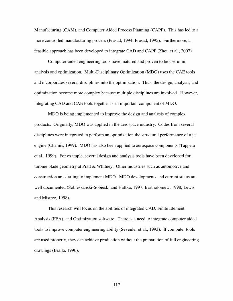
the automation loop is shown in figure 4.

121

Figure 4: Automation Loop Flowchart for VBSA

This automation requires various software packages. First, i-Sight FD® was

utilized to control the entire design loop. For the VBSA, this software reads the input

data from an input file and writes the results to a results file. Both of these files are text

files that can easily be manipulated. For the optimization, i-Sight FD® is used to specify

the optimization scheme its initial criteria. i-Sight FD® also launches the other software

packages that are required for the automation loop. The loop in i-Sight FD® is shown in

figure 5.

Figure 5: i-Sight FD® Automation Loop

Other software needed for the automation loop includes Unigraphics® and

ANSYS®. Unigraphics® controls the parametric model. A feature library based design

tool was created using the Unigraphics® Application Program Interface (API) that

122

quickly generates robust, parametric BOAS geometry. The user selects different features

of a BOAS and the design tool imports them into a seed model to create a complete

BOAS model. All the features are parametric and the user specifies the parameter values

for each feature. Thus, the result is a fully parametric model. This geometry is then

updated for each design point by the first two components, “Expression Parse” and

“Unigraphics”, in the automation loop as shown in figure 5.

Similarly, ANSYS® handles the analysis portion of the loop. The ANSYS® API,

which is the ANSYS® Parametric Design Language (APDL), was utilized to automate the

entire analysis. The APDL provides the full functionality of the ANSYS Graphical User

Interface (GUI). Thus, the analysis tool that was developed is a program that automates

what an engineer would do manually. Both structural and thermal analyses are executed.

They are seamlessly integrated and the analysis automation tool imports the geometry,

analyzes it, and writes the results to a text file without any human involvement. The last

components of the automation loop in figure 5, “ANSYS” and “ANSYS Results Parse”,

run the analysis program and store the results. The remaining components; “Grain

Orientation and Wall Thickness Calc”, “Grain Orientation Parse”, and “Wall Thickness

Parse”, perform calculations that are required for the analysis. Thus, the entire

automation loop takes input parameters, updates the parametric model, runs the analysis,

and stores the results on a text file.

Without this automation loop, a VBSA or optimization could not be conducted. It

would take too long to manually create and analyze the number of different designs

required for a VBSA or optimization. Furthermore, it would be too expensive to run the

123

physical experiments. Therefore, automating the design and analysis process to

implement MDO is required before a VBSA or optimization can be realistically utilized.

4 VBSA Preparation and Approach

An automation loop makes a VBSA possible and the configuration of a VBSA

depends on the question that needs to be answered.

4.1 Input Parameters

There were seven input factors chosen for this research. For the BOAS, these

factors were chosen based on expert opinion. It is expected that these parameters affect

Scallop LCF Life. However, it is unknown as to the level of importance for each factor.

Of the seven input parameters, four are geometric parameters and three define grain

orientation. The four geometric parameters are defined in figure 6, which is a cross

section of figure 2.

Figure 6: BOAS Geometric Input Parameters

The reference plane in figure 6 is a fixed plane that is used to define geometric

parameters. The parameters Core Radial Placement and Core Radial Thickness control

all the cores. Thus, each core has the same Core Radial Thickness value. ID Grind

controls the locations of the inner diameter surface relative to the reference plane and

Panel Placement defines where the main panel is placed.

124

The nominal grain orientation direction is along the x axis. There are three grain

orientation parameters, Alpha, Beta, and Secondary Grain Orientation (SGO), which are

varied relative to the nominal grain orientation direction. Together, these parameters

fully define the grain orientation.

4.2 Bounds on Input Parameters

There are three different sets of inputs bounds. The sets include manufacturing

sensitivity analysis bounds, design sensitivity analysis bounds, and a final set for the

design optimization. The goal of the manufacturing sensitivity analysis is to find the

parameters that cause the variation seen in physical parts. Thus, the input parameters

were measured on actual parts to get their respective distributions. Both the histograms

and probability density functions indicated that the data follows a Gaussian distribution.

Therefore, the mean was calculated and the input bounds were set to be ±3� from the

mean. Another option is to use blueprint tolerances bounds and that it is not necessary to

measure physical parts. Unfortunately, the values that exist for a parameter on

manufactured parts may not be the same as the blueprint tolerances. Therefore, it is

important to gather actual part data. Figure 7 illustrates the difference between blueprint

tolerances and physical part data by showing that the nominal Panel Placement value is

never manufactured.

125

Figure 7: Panel Placement Data and Bounds

The goal of the design sensitivity analysis is to discover which parameters are

most important in terms of design. The ultimate goal with the design sensitivity analysis

and the optimization is to find the optimal part design. Thus, the bounds on the input

parameters were enlarged beyond the manufacturing sensitivity analysis bounds and

blueprint tolerances. The bounds were determined based on physical considerations. For

example, Core Radial Thickness cannot be too small since it cannot be manufactured so

there is a corresponding lower bound on Core Radial Thickness. Also, a sensitivity

analysis requires fixed bounds, not relative bounds. For example, the limit of Core

Radial Placement is dependent on ID Grind. For the VBSA, fixed bounds were

developed so Core Radial Placement would not extend past ID Grind. For the

optimization, constraints were developed such that the upper limit of Core Radial

Placement depends on ID Grind parameter. The optimization constraints are discussed in

greater detail in section VII of this paper.

126

4.3 Design Space

To fill the design space for the sensitivity analyses, a Latin hypercube, which is a

design space filling technique, was utilized (Santner et al., 2003). A Latin hypercube

requires that each input factor be divided into n bins. Next, each bin is filled with exactly

one design point. Finally, the minimum distance between all design points is maximized

and this is referred to as the max-min criteria. This provides a method to evenly populate

the entire design space. A Latin hypercube typically requires a large number of design

points. This is not a problem because the automation loop ensures that analyzing all the

designs points in not time consuming for the engineer. To create the Latin Hypercube

design for the BOAS research, Gaussian Emulation Machine for Sensitivity Analysis

(GEM-SA) software was used. This software was developed by Marc Kennedy for the

Centre for Terrestrial Carbon Dynamics (CTCD) (Kennedy and O’Hagan, 2006;

Kennedy and O’Hagan, 2001). This software only requires the following information:

the number of input variables, number of design points, and the variable bounds. It then

generates a Latin Hypercube design using the max-min criteria. For the optimization, no

space filling technique is needed and several optimization algorithms were implemented.

4.4 Gathering of Results

The results of both sensitivity analyses were stored individually after running the

automation loop. With this data, the GEM-SA software was utilized to create plots

listing the relative importance of each factor (Kennedy, O’Hagan, 2006). Also, plots

showing the change in Scallop LCF Life against the input parameters are created. For the

optimization, the data for the first, last, and all intermittent designs is stored. Thus, the

data can be processed to analyze the optimization results.

127

5 Manufacturing Sensitivity Analysis Results

The goal of the manufacturing sensitivity analysis is to discover what parameters

are causing the variation in Scallop LCF Life in physical BOAS. Figure 8 shows a Pareto

plot that depicts which parameters are most important from a manufacturing sense.

Scallop LCF Life

0

10

20

30

40

50

60

Core Rad

ial P

lacem

ent

SGOAlph

a

ID G

rind

Core Rad

ial P

lacem

ent.S

GO

Core Rad

ial P

lacem

ent.A

lpha

SGO.Alph

a

Core Rad

ial P

lacem

ent.ID

Grin

d

Panel

Positio

n

Per

cent

Effe

ct

Figure 8: Scallop LCF Life Pareto Plot for Manufacturing Sensitivity Analysis

Figure 8 clearly shows that Core Radial Placement in the most important parameter.

Thus, reduction in the variation in Scallop LCF Life can be achieved by reducing the

manufacturing variation that is seen in Core Radial Placement. However, the engineers

also need to know what values of Core Radial Placement result in higher Scallop LCF

Life. This is shown in figure 9.

128

Normalized Scallop LCF Life vs Normalized Core Radial Placement

0

0.1

0.2

0.3

0.4

0.5

0.6

0.7

0.8

0.9

1

0 0.1 0.2 0.3 0.4 0.5 0.6 0.7 0.8 0.9 1

Normalized Core Radial Placement

Nor

mal

ized

Sca

llop

LCF

Life

Figure 9: Normalized Scallop LCF Life versus Normalized Core Radial Placement

The data is figure 9 is normalized to be between 0 and 1 due to proprietary

concerns. It illustrates that Scallop LCF Life increases as Core Radial Placement

increases. As Core Radial Placement increases, the cores are closer to the inner diameter

surface. Therefore, the inner diameter surface is cooler and the compressive stress in the

scallops is lower. This results in a larger Scallop LCF Life value. Thus, the engineers

should seek to control the manufacturing process to ensure that Core Radial Placement

values are relatively high. This will improve part reliability and provide consistent

performance.

6 Design Sensitivity Analysis Results

The goal of the design sensitivity analysis is to discover which parameters are

important in terms of Scallop LCF Life. Thus, the unimportant factors can be removed

from the optimization. This will reduce the computational time required for the

optimization. The results for the sensitivity analysis are shown in a Pareto plot in figure

10.

129

Figure 10: Scallop LCF Life Pareto Plot for Design Sensitivity Analysis

The results in figure 10 differ than the results shown in figure 8. This is due to

the design space being enlarged. Since the parameters are allowed to vary more, it is not

surprising that the results are not the same. One major difference is that the results for

the design sensitivity analysis are more complicated. Three of the top four most

important parameters are two factor interaction effects. In the manufacturing sensitivity

analysis, the four most important factors were all main effects.

From figure 10, it is possible to obtain the important factors for the optimization.

These are Alpha, Beta, Core Radial Placement, Core Thickness, and ID Grind. These

will be the design variables in the optimization

130

7 Optimization

Optimizations find the best performing design. However, this design may

experience sharp declines in performance if the input parameters slightly deviate from

their optimal values. Optimization results should be carefully analyzed before they are

accepted.

7.1 Formulation

The optimization formulation is shown in equation 1.

11

1010

101010

__:minimize

≤≤

≤≤≤≤

≤≤≤≤≤≤

−

ergyIDStrainEn

emperatureIDSurfaceT

IDGrind

essCoreThickn

PlacemntCoreRadial

LifeLCFScallop

βα

(1)

Due to proprietary considerations, the actual equations and constraint bounds

cannot be disclosed. Thus, all the data is normalized to be between 0 and 1.

To solve this optimization problem, several techniques were utilized. These

schemes include Hookes-Jeeves (Reklaitis et al., 1986), Large Scale Generalized

Reduced Gradient (LSGRG) (Smith and Lasdon, 1992), and Multi-Island Genetic

Algorithm (GA) (Niwa and Tanaka, 1999). These schemes were chosen because they

exhibit fundamentally different approaches. The Hookes-Jeeves approach is a direct

penalty method while the LSGRG is a direct numerical technique that relies on the

gradient of the design space. Finally, the Multi-Island GA is an exploratory technique.

131

7.2 Results

Before the optimization was conducted, the design sensitivity analysis was

analyzed. This analysis reveals the probable solution. Figure 11 depicts the scallop

compressive stress against each of the input values. Scallop compressive stress is the

main driver of Scallop LCF Life and it is used in these plots because the Scallop LCF

Life widely varies. A small change in scallop compressive stress can result in drastic

shift in Scallop LCF Life. Thus, if Scallop LCF Life is plotted against an input value, it

is difficult to see the trend.

Normalized Scallop Compressive Stress vs Normalized Alpha

0

0.1

0.2

0.3

0.4

0.5

0.6

0.7

0.8

0.9

1

0 0.1 0.2 0.3 0.4 0.5 0.6 0.7 0.8 0.9 1

Normalized Alpha

Nor

mal

ized

Sca

llop

Com

pres

sive

Str

ess

Normalized Scallop Compressive Stress vs Normalized Beta

0

0.1

0.2

0.3

0.4

0.5

0.6

0.7

0.8

0.9

1

0 0.1 0.2 0.3 0.4 0.5 0.6 0.7 0.8 0.9 1

Normalized Beta

Nor

mal

ized

Sca

llop

Com

pres

sive

Str

ess

132

Normalized Scallop Compressive Stress vs Normalized Core Radial Placement

0

0.1

0.2

0.3

0.4

0.5

0.6

0.7

0.8

0.9

1

0 0.1 0.2 0.3 0.4 0.5 0.6 0.7 0.8 0.9 1

Normalized Core Radial Placement

Nor

mal

ized

Sca

llop

Com

pres

sive

Str

ess

Normalized Scallop Compressive Stress vs Normalized Core Thickness

0

0.1

0.2

0.3

0.4

0.5

0.6

0.7

0.8

0.9

1

0 0.1 0.2 0.3 0.4 0.5 0.6 0.7 0.8 0.9 1

Normalized Core Thickness

Nor

mal

ized

Sca

llop

Com

pres

sive

Str

ess

Normalized Scallop Compressive Stress vs Normalized ID Grind

0

0.1

0.2

0.3

0.4

0.5

0.6

0.7

0.8

0.9

1

0 0.1 0.2 0.3 0.4 0.5 0.6 0.7 0.8 0.9 1

Normalized ID Grind

Nor

mal

ized

Sca

llop

Com

pres

sive

Str

ess

Figure 11: Normalized Scallop Compressive Stress vs Normalized Alpha, Beta, Core Radial

Placement, Core Thickness, and ID Grind

133

Lower scallop compressive stress results in a greater Scallop LCF Life. Thus, the

optimal design is expected to minimize � and maximize ID Grind. Unfortunately, it is

unclear what �, Core Radial Placement, and Core Thickness should be. However,

analyzing material thickness, which is the distance between the cores and the inner

diameter surface, assists in finding a likely optimal point for Core Radial Placement.

Normalized Scallop Compressive Stress vs Normalized Material Thickness

0

0.1

0.2

0.3

0.4

0.5

0.6

0.7

0.8

0.9

1

0 0.1 0.2 0.3 0.4 0.5 0.6 0.7 0.8 0.9 1

Normalized Material Thickness

Nor

mal

ized

Sca

llop

Com

pre

ssiv

e S

tres

s

Figure 12: Normalize Scallop Compressive Stress vs Normalized Material Thickness

Figure 12 shows that a lower material thickness results in a smaller scallop

compressive stress. Therefore, the cores should be as close to the inner diameter surface

as possible. The analysis of the design sensitivity analysis will assist to verify the

optimization results.

The first optimizations that were conducted utilized the Hookes-Jeeves and

LSGRG schemes. These runs revealed what optimal values for �, �, and Core Radial

Placement. Core Radial Placement should be as close to the ID Grind surface as possible

while � and � should be 0. Both of these solutions are supported by the design sensitivity

analysis.

134

Unfortunately, the optimizations produced different results for ID Grind and Core

Thickness. The results varied depending on the initial point and the optimization

technique. To solve this issue, the optimization was reduced to two input parameters, ID

Grind and Core Thickness. The remaining input factors were set to their respective

optimal values. However, the Hookes-Jeeves and LSGRG techniques gave different

results depending on the initial value. The schemes located local minima instead of the

optimal solution. To find the optimal ID Grind and Core Thickness values, the Multi-

Island GA technique was applied. This scheme was successful and the results are shown

in the next two figures.

0 0.1 0.2 0.3 0.4 0.5 0.6 0.7 0.8 0.9 10

0.1

0.2

0.3

0.4

0.5

0.6

0.7

0.8

0.9

1

Normalized Core Thickness

Nor

mal

ized

Sca

llop

LCF

Life

Normalized Scallop LCF Life vs Normalized Core Thickness

ValidViolates Constraints

Figure 13: Normalized Scallop LCF Life vs Normalized Core Thickness

135

0 0.1 0.2 0.3 0.4 0.5 0.6 0.7 0.8 0.9 10

0.1

0.2

0.3

0.4

0.5

0.6

0.7

0.8

0.9

1

Normalized ID Grind

Nor

mal

ized

Sca

llop

LCF

Life

Normalized Scallop LCF Life vs Normalized ID Grind

ValidViolates Constraints

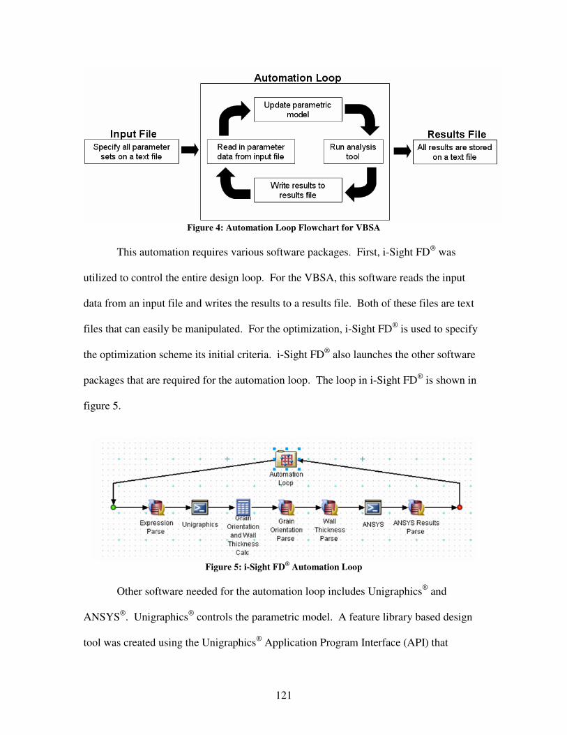
Figure 14: Normalized Scallop LCF Life vs Normalized ID Grind

Figures 13 and 14 show that Core Thickness should be minimized and ID Grind

should be maximized. However, before either can reach their respective extreme, the

constraints are violated. Clearly, the Multi-Island GA found the approximate solution.

To find the exact solution, Hookes-Jeeves and LSGRG were ran again with the general

GA solution as the starting point. Both found a more precise optimal solution. Thus, the

optimal scaled input values are:

79.014.0

91.000

==

===

IDGrind

essCoreThickn

PlacementCoreRadial

βα

8 Conclusions

The creation of an automation loop provides new capabilities for engineers. The

engineer can analyze the manufacturing process by conducting a VBSA. This provides

136

information detailing which input parameters cause variation in currently produced

products. Furthermore, a VBSA can be run from a design point of view. This

information, in conjunction with an optimization, allows the engineer to design a product

with greater performance. However, the optimization should be carefully analyzed. The

results may not necessarily be the true optimal design and great care should be taken

before the results are believed.

Acknowledgements

A special thanks to Pratt & Whitney for their support and expertise. They

provided programs that were used and modified for this work. Furthermore, Pratt &

Whitney employees answered technical questions and offered their insights on the proper

method to develop the design, analysis, and automation tools. Finally, thanks to ANSYS

Inc. for providing ANSYS® Academic Research v11.0.

137

References

ANSYS® Academic Research, v 11.0. Bartholomew, P., “The Role of MDO within Aerospace Design and Progress Towards an

MDO Capability,” AIAA Paper 98-4705, 7th AIAA/USAF/NASA/ISSMO Symposium on Multi-disciplinary Analysis and Optimization, St. Louis, MO, September 1998.

Bralla, J. G., Design for Excellence, USA: McGraw-Hill, 1996.

Chamis, C. C., “Coupled Multidisciplinary Optimization of Engine Structural Performance,” Journal of Aircraft, Vol. 36, No.1, 1999, pp. 190-199.

Kennedy, M., O’Hagan T., “Bayesian Calibration of Computer Models,” Journal of the

Royal Statistical Society, Series B, Vol. 63, Part 3, 2001, pp. 425-464. Kennedy, M., O’Hagan T., http://www.tonyohagan.co.uk/academic/GEM, 2006. Lewis, K., and Mistree, F., “The Other Side of Multidisciplinary Design Optimization:

Accommodating a Multiobjective, Uncertain, and Non-Deterministic World,” Engineering Optimization, Vol. 31, 1998, pp. 161-189.

Niwa, T., and Tanaka, M., “Analysis on the Island Model Parallel Genetic Algorithms for

the Genetic Drifts,” Lecture Notes in Computer Science, Vol. 1585, 1999, pp. 349-356.

Prasad, B., “Product Planning Optimization Using Quality Function Deployment”, in AI

in Optimal Design & Manufacturing,. Z. Dong, (ed.) and series ed. Mo. Jamshidi. Englewood, NJ: Prentice Hall, 1993, pp. 117-152.

Prasad, B., “Competitiveness Analysis of Early Product Introduction and Technology

Insertion,” Proceedings of the 1994 Int’l Mechanical Engineering Congress and Exposition, Nov. 1994, Chicago, IL. PED-Vol. 68-1, Manufacturing Science and Engineering, Col. 1, ASME, 1994, pp. 121-134.

Prasad, B., “A Structured Approach to Product and Process Optimization for

Manufacturing and Service Industries,” International Journal of Quality and Reliability Management, Vol. 12, No. 9, 1995.

Reklaitis, G., Ravindran, A., Ragsdell, K., Engineering Optimization Methods and

Applications, USA: John Wiley & Sons, Inc., 1983. Santner, T., Williams, B., Notz, W., The Design and Analysis of Computer Experiments,

USA: Springer, 2003.

138

Sevenler, K., Sherman, M. K. and Vidal, R., “Multidisciplinary Teamwork in Product Design: Some Requirement for Computer Systems,” ICED, 1993, pp. 343.

Smith S., and Lasdon L., “Solving Large Sparse Nonlinear Programs using GRG,”

ORSA J., Comput. 4, 1992, pp. 1-15. Sobieszanski-Sobieski, J., and Haftka, R., “Multidisciplinary Aerospace Design

Optimization: Survey of Recent Developments,” Structural Optimization, Vol. 14, 1997, pp. 1-23.

Tappeta, R. V., Nagendra, S., and Renaud, J. E., “A Multidisciplinary Design

Optimization Approach for High Temperature Aircraft Engine Components,” Structural Optimization, Vol. 18, 1999, pp. 134-145.

United Technologies- Pratt & Whitney, “PW4000 94-Inch Fan Engine,”

http://www.pw.utc.com Zhou, X., Yanjie, Q., Guangru, H,. Huifeng, W., Xueyu, R,. “A feasible approach to the

integration of CAD and CAPP,” Computer-Aided Design, Vol. 39, 2007, pp. 324-338.