APPLICATION OFAPPLICATION OFAPPLICATION OFAPPLICATION OF

VIRTUAL INSTRUMENTATION & LABVIEWVIRTUAL INSTRUMENTATION & LABVIEWVIRTUAL INSTRUMENTATION & LABVIEWVIRTUAL INSTRUMENTATION & LABVIEW

IN COMMUNICATION SYSYTEMS

AA PPRROOJJEECCTT RREEPPOORRTT

Submitted in partial fulfillment of the requirements for the award of the degree of

BACHELOR OF TECHNOLOGY IN

ELECTRONICS AND INSTRUMENTATION ENGINEERING

by

SOUMYA RANJAN PANDA (10307007)

AVINASH MOHANTY (10307028)

Department of Electronics and Instrumentation Engineering

NNaattiioonnaall IInnssttiittuuttee OOff TTeecchhnnoollooggyy,, RRoouurrkkeellaa

Pin-769008, Orissa, INDIA

22000066 –– 22000077

APPLICATION OFAPPLICATION OFAPPLICATION OFAPPLICATION OF

VIRTUAL INSTRUMENTATION & LVIRTUAL INSTRUMENTATION & LVIRTUAL INSTRUMENTATION & LVIRTUAL INSTRUMENTATION & LABVIEWABVIEWABVIEWABVIEW

IN COMMUNICATION SYSYTEMS

AA PPRROOJJEECCTT RREEPPOORRTT

Submitted in partial fulfillment of the requirements for the award of the degree of

BACHELOR OF TECHNOLOGY IN

ELECTRONICS AND INSTRUMENTATION ENGINEERING

by

SOUMYA RANJAN PANDA (10307007)

AVINASH MOHANTY (10307028)

Under the guidance of DDrr..SS..KK..PPAATTRRAA

Department of Electronics and Instrumentation Engineering

NNaattiioonnaall IInnssttiittuuttee OOff TTeecchhnnoollooggyy,, RRoouurrkkeellaa

Pin-769008, Orissa, INDIA

22000066 –– 22000077

National Institute of Technology

Rourkela

CERTIFICATE

This is to certify that the thesis entitled, “Application of virtual instrumentation & labview in communication systems” submitted by Sri Soumya Ranjan Panda and Sri Avinash Mohanty in partial fulfillments for the requirements for the award of Bachelor of Technology Degree in Electronics & Instrumentation Engineering at National Institute of Technology, Rourkela (Deemed University) is an authentic work carried out by him under my supervision and guidance.

To the best of my knowledge, the matter embodied in the thesis has not been submitted to

any other University / Institute for the award of any Degree or Diploma.

Date: Prof. S. K. PATRA

Dept. of Electronics & Instrumentation Engg

National Institute of Technology

Rourkela - 769008

ACKNOWLEDGEMENT

We place on record and warmly acknowledge the continuous encouragement,

invaluable supervision, timely suggestions and inspired guidance offered by our guide Prof.

S.K.Patra, Professor, Department of Electronics and instrumentation Engineering, National

Institute of Technology, Rourkela, in bringing this report to a successful completion.

We are grateful to Prof. G.Panda, Head of the Department of Electronics and

instrumentation Engineering, for permitting us to make use of the facilities available in the

department to carry out the project successfully. Last but not the least we express our sincere

thanks to all of our friends who have patiently extended all sorts of help for accomplishing this

undertaking.

Finally we extend our gratefulness to one and all who are directly or indirectly

involved in the successful completion of this project work.

.

Soumya Ranjan Panda(10307007)

Avinash Mohanty(10307028)

i

CONTENTS Page No

Abstract ii

Chapter 1 GENERAL INTRODUCTION 1-7

1.1 Virtual Instruments 2

1.2 Dataflow Programming 3

1.3 Graphical Programming 4

1.4 Benefits & criticism 4

Chapter2 BASICS OF COMMUNICATION 8-14

2.1 Frequency translation 9

2.2 Multiple frequency translation 11

2.3 SSaammppll iinngg tthheeoorreemm ((nnyyqquuiisstt ccrrii tteerriioonn)) 13

Chapter3 AMPLITUDE MODULATION 15-24

3.1 Amplitude modulation and demodulation 16

3.2 Multiple Amplitude modulation 19

3.3 DSB-SC generation 21

3.4 SSB Amplitude Modulation 23

Chapter 5 PULSE MODULATION 25-31

4.1 Pulse Amplitude Modulation (PAM) 26

4.2 Pulse Width Modulation (PWM) 28

4.3 Pulse Position Modulation (PPM) 30

Chapter 6 ADVANCE COMMUNICATION TECHNIQUES 32-39

5.1 Time Division Multiplexing (TDM) 33

5.2 Frequency Division Multiplexing (FDM) 36

5.3 Amplitude Shift Key (ASK) 38

REFERENCES 40

ii

ABSTRACT

Introduction:

Virtual instrumentation:

Virtual Instrumentation is the use of customizable software and modular measurement hardware

to create user-defined measurement systems, called virtual instruments. The concept of a

synthetic instrument is a subset of the virtual instrument concept. A synthetic instrument is a

kind of virtual instrument that is purely software defined. A synthetic instrument performs a

specific synthesis, analysis, or measurement function on completely generic, measurement

agnostic hardware. Virtual instruments can still have measurement specific hardware, and tend to

emphasize modular hardware approaches that facilitate this specificity. Hardware supporting

synthetic instruments is by definition not specific to the measurement, nor is it necessarily (or

usually) modular.

Leveraging commercially available technologies, such as the PC and the analog to digital

converter, virtual instrumentation has grown significantly since its inception in the late 1970s.

Additionally, software packages like National Instruments' Lab VIEW and other graphical

programming languages helped grow adoption by making it easier for non-programmers to

develop systems.

Lab VIEW:

Lab VIEW (short for Laboratory Virtual Instrumentation Engineering Workbench)

is a platform and development environment for a visual programming language from National

Instruments. Originally released for the Apple Macintosh in 1986, Lab VIEW is commonly used

for data acquisition, instrument control, and industrial automation on a variety of platforms

including Microsoft Windows, various flavors of UNIX, Linux, and Mac OS.The programming

language used in Lab VIEW, is a dataflow language. Execution is determined by the structure of

a graphical block diagram.

iii

Lab VIEW (short for Laboratory Virtual Instrumentation Engineering Workbench) is a

platform and development environment for a visual programming language from National

Instruments.

Since this might be the case for multiple nodes simultaneously, it is inherently capable

of parallel execution. Furthermore, Lab VIEW does not require type definition of the variables;

the wire type is defined by the data-supplying node.

Communication systems:

Starting from the easiest of the communication techniques and systems we move

towards the most complicated and explore the use of virtual instrumentation and lab VIEW and

its scope in creating a close simulation of these systems. The techniques covered begin from

normal frequency translation to amplitude modulation leading to pulse modulation and finally

culminates in the simulation of tougher topics like that of time and frequency division

multiplexing and amplitude shift keying.

Experimental work

� Lab VIEW ties the creation of user interfaces (called front panels) into the development

cycle. Lab VIEW programs/subroutines are called virtual instruments (VIs). Each VI has

three components:

� Block diagram

� Connector pane

� Front panel

However, the front panel can also serve as a programmatic interface. This implies each VI can

be easily tested before being embedded as a subroutine into a larger program

The graphical approach also allows non-programmers

to build programs by simply dragging and dropping virtual representations of the lab equipment

with which they are already familiar. The Lab VIEW programming environment, with the

included examples and the documentation, makes it simpler to create small applications. This is a

benefit on one side but there is also a certain danger of underestimating the expertise needed for

good quality programming.

1

Chapter 1

AN INTRODUCTION TO LAB VIEW AND

VIRTUAL INSTRUMENTATION

2

Virtual instrumentation

Virtual Instrumentation is the use of customizable software and modular measurement hardware

to create user-defined measurement systems, called virtual instruments.

'Traditional' or 'natural' instrumentation systems are made up of pre-defined hardware components,

such as digital multimeters and oscilloscopes that are completely specific to their stimulus, analysis,

or measurement function. Because of their hard-coded function, these systems are more limited in

their versatility than virtual instrumentation systems. The primary difference between 'natural'

instrumentation and virtual instrumentation is the software component of a virtual instrument. The

software enables complex and expensive equipment to be replaced by simpler and less expensive

hardware; e.g. analog to digital converter can act as a hardware complement of a virtual

oscilloscope, a potentiostat enables frequency response acquisition and analysis in electrochemical

impedance spectroscopy with virtual instrumentation.

The concept of a synthetic instrument is a subset of the virtual instrument concept. A synthetic

instrument is a kind of virtual instrument that is purely software defined. A synthetic instrument

performs a specific synthesis, analysis, or measurement function on completely generic,

measurement agnostic hardware. Virtual instruments can still have measurement specific hardware,

and tend to emphasize modular hardware approaches that facilitate this specificity. Hardware

supporting synthetic instruments is by definition not specific to the measurement, nor is it

necessarily (or usually) modular.

Leveraging commercially available technologies, such as the PC and the analog to digital converter,

virtual instrumentation has grown significantly since its inception in the late 1970s. Additionally,

software packages like National Instruments' LabVIEW and other graphical programming

languages helped grow adoption by making it easier for non-programmers to develop systems.

3

Lab VIEW

(acronym for Laboratory Virtual Instrumentation Engineering Workbench) is a platform and

development environment for a visual programming language from National Instruments. The

graphical language is named "G". Originally released for the Apple Macintosh in 1986, LabVIEW

is commonly used for data acquisition, instrument control, and industrial automation on a variety of

platforms including Microsoft Windows, various flavors of UNIX, Linux, and Mac OS. The latest

version of LabVIEW is version 8.20, released in honor of LabVIEW's 20th anniversary.

Dataflow programming

The programming language used in LabVIEW, called "G", is a dataflow language. Execution is

determined by the structure of a graphical block diagram (the LV-source code) on which the

programmer connects different function-nodes by drawing wires. These wires propagate variables

and any node can execute as soon as all its input data become available. Since this might be the case

for multiple nodes simultaneously, G is inherently capable of parallel execution. Multi-processing

and multi-threading hardware is automatically exploited by the built-in scheduler, which

multiplexes multiple OS threads over the nodes ready for execution.

Programmers with a background in conventional programming often show a certain reluctance to

adopt the LabVIEW dataflow scheme, claiming that LabVIEW is prone to race conditions. In

reality, this stems from a misunderstanding of the data-flow paradigm. The aforementioned data-

flow (which can be "forced", typically by linking inputs and outputs of nodes) completely defines

the execution sequence, and that can be fully controlled by the programmer. Thus, the execution

sequence of the LabVIEW graphical syntax is as well defined as with any textually coded language

such as C, Visual BASIC, and Python etc. Furthermore, LabVIEW does not require type definition

of the variables; the wire type is defined by the data-supplying node. LabVIEW supports

polymorphism in that wires automatically adjust to various types of data.

4

Graphical programming

LabVIEW ties the creation of user interfaces (called front panels) into the development cycle.

LabVIEW programs/subroutines are called virtual instruments (VIs). Each VI has three

components: a block diagram, a front panel and a connector pane. The latter may represent the VI as

a subVI in block diagrams of calling VIs. Controls and indicators on the front panel allow an

operator to input data into or extract data from a running virtual instrument. However, the front

panel can also serve as a programmatic interface. Thus a virtual instrument can either be run as a

program, with the front panel serving as a user interface, or, when dropped as a node onto the block

diagram, the front panel defines the inputs and outputs for the given node through the connector

pane. This implies each VI can be easily tested before being embedded as a subroutine into a larger

program.

The graphical approach also allows non-programmers to build programs by simply dragging and

dropping virtual representations of the lab equipment with which they are already familiar. The

LabVIEW programming environment, with the included examples and the documentation, makes it

simpler to create small applications. This is a benefit on one side but there is also a certain danger of

underestimating the expertise needed for good quality "G" programming. For complex algorithms

or large-scale code it is important that the programmer possess an extensive knowledge of the

special LabVIEW syntax and the topology of its memory management. The most advanced

LabVIEW development systems offer the possibility of building stand-alone applications.

Furthermore, it is possible to create distributed applications which communicate by a client/server

scheme, and thus is easier to implement due to the inherently parallel nature of G-code.

Benefits

One benefit of LabVIEW over other development environments is the extensive support for

accessing instrumentation hardware. Drivers and abstraction layers for many different types of

instruments and buses are included or are available for inclusion. These present themselves as

graphical nodes. The abstraction layers offer standard software interfaces to communicate with

hardware devices. The provided driver interfaces save program development time. The sales pitch

of National Instruments is, therefore, that even people with limited coding experience can write

5

programs and deploy test solutions in a reduced time frame when compared to more conventional or

competing systems. A new hardware driver topology (DAQmxBase), which consists mainly of G-

coded components with only a few register calls through NI Measurement Hardware DDK (Driver

Development Kit) functions, provides platform independent hardware access to numerous data

acquisition and instrumentation devices. The DAQmxBase driver is available for LabVIEW on

Windows, MacOSX and Linux platforms.

In terms of performance, LabVIEW includes a compiler that produces native code for the CPU

platform. The graphical code is translated into executable machine code by interpreting the syntax

and by compilation. The LabVIEW syntax is strictly enforced during the editing process and

compiled into the executable machine code when requested to run or upon saving. In the latter case,

the executable and the source code are merged into a single file. The executable runs with the help

of the LabVIEW run-time engine, which contains some precompiled code to perform common tasks

that are defined by the G language. The run-time engine reduces compile time and also provides a

consistent interface to various operating systems, graphic systems, hardware components, etc. The

run-time environment makes the code portable across platforms. Generally, LV code can be slower

than equivalent compiled C code, although the differences often lie more with program optimization

than inherent execution speed.

Many libraries with a large number of functions for data acquisition, signal generation,

mathematics, statistics, signal conditioning, analysis, etc., along with numerous graphical interface

elements are provided in several LabVIEW package options.

The LabVIEW Professional Development System allows creating stand-alone executables and the

resultant executable can be distributed an unlimited number of times. The run-time engine and its

libraries can be provided freely along with the executable.

A benefit of the LabVIEW environment is the platform independent nature of the G-code, which is

(with the exception of a few platform-specific functions) portable between the different LabVIEW

systems for different operating systems (Windows, MacOSX and Linux). National Instruments is

increasingly focusing on the capability of deploying LabVIEW code onto an increasing number of

6

targets including devices like Phar Lap OS based LabVIEW real-time controllers, PocketPCs,

PDAs, Field Point modules and into FPGAs on special boards.

There is a low cost LabVIEW Student Edition aimed at educational institutions for learning

purposes. There is also an active community of LabVIEW users who communicate through several

e-mail groups and Internet forums.

Criticism

LabVIEW is a proprietary product of National Instruments. Unlike common programming

languages such as C or FORTRAN, LabVIEW is not managed or specified by a third party

standards committee such as ANSI. Obtaining a fully compatible and up to date LabVIEW platform

requires purchasing the product. There is a movement to create user-defined extensions for the

development environment at OpenG.org but an initial purchase of LabVIEW is still required.

Currently there is no open source, free software or alternative commercial program that can

implement any portion of G-code.

In addition, as of version 8, all LabVIEW installs require customers to contact National Instruments

by Internet or phone to "activate" the product. The increasing dependence on the vendor suggests

possible privacy and data security concerns. For example, although National Instruments claims the

process is "secure and anonymous" the immediate implication is that a legal but privately installed

instance of LabVIEW seems no longer possible. However, if National Instruments were to go out of

business, the LabVIEW code is escrowed and would be released to the public, and so there would

be no concerns over activation. This would mean that, with the current system, the user would no

longer be able to access their code base as well as certain formats of archived data.

Building a stand-alone application with LabVIEW requires the Application Builder component

which is included with the Professional Development System but requires a separate purchase if

using the Base Package or Full Development System. Compiled executables produced by the

Application Builder are not truly standalone in that they also require that the LabVIEW run-time

engine be installed on any target computer on which users run the application. Although this run-

7

time engine can be freely downloaded from National Instruments' website, this added requirement is

in contrast to other compiled languages, such as C, where a stand-alone executable file can be

created, run and distributed without the need for additional files or installation procedures. These

requirements can cause problems if an application is distributed to a user who may be prepared to

run the application but does not have the inclination or permission to install additional files on the

host system prior to running the executable. The need for a separately installed LabVIEW run-time

engine makes the development and distribution of truly portable applications using LabVIEW

difficult.

There is some debate as to whether LabVIEW is really a general-purpose programming

language (or in some cases whether it is really a programming language at all) as opposed to an

application-specific development environment for measurement and automation. Critics point to a

lack of features, common in most other programming languages, such as native recursion and, until

version 8.20, object oriented features. While it is possible to write complex applications in

LabVIEW that involve no measurement or automation, it is not best suited to the task

8

Chapter 2

BASICS OF COMMUNICATION SYSTEMS

9

Frequency translation

Theory:

It is often advantageous and convenient, in processing a signal in a communication system, to

translate the signal from one region in frequency domain to another region. Suppose that a signal

having a frequency f1,the frequency translation is one in which original signal is replace with a new

signal whose spectral range extends from f1’ to f2’ and new signal has the same information as that

of the original signal..

Some of the useful purposes which may be served by frequency translation are:

� Frequency Multiplexing

� Practicability of Antennas

� Narrowbanding

A signal may be translated to a new spectral range by multiplying the signal with an auxiliary

sinusoidal signal. Let us consider initially the signal be

Vm(t)= Amcos ωmt

Carrier signal

Vc(t)=Accos ωct

Frequency translated signal:

VVmm((tt))VVcc((tt))==KK ((ee jj((ωωcc++ωωmm))tt ++ ee --jj((ωωcc++ωωmm))tt++ ee jj((ωωcc--ωωmm))tt ++ ee --jj((ωωcc--ωωmm))tt ))

10

Block diagram

Front Panel

11

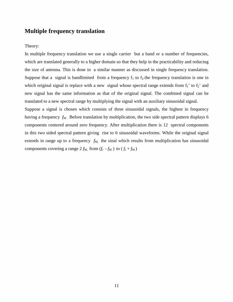
Multiple frequency translation

Theory:

In multiple frequency translation we use a single carrier but a band or a number of frequencies,

which are translated generally to a higher domain so that they help in the practicability and reducing

the size of antenna. This is done in a similar manner as discussed in single frequency translation.

Suppose that a signal is bandlimited from a frequency f1 to f2.the frequency translation is one in

which original signal is replace with a new signal whose spectral range extends from f1’ to f2’ and

new signal has the same information as that of the original signal. The combined signal can be

translated to a new spectral range by multiplying the signal with an auxiliary sinusoidal signal.

Suppose a signal is chosen which consists of three sinusoidal signals, the highest in frequency

having a frequency fM . Before translation by multiplication, the two side spectral pattern displays 6

components centered around zero frequency. After multiplication there is 12 spectral components

in this two sided spectral pattern giving rise to 6 sinusoidal waveforms. While the original signal

extends in range up to a frequency fM, the sinal which results from multiplication has sinusoidal

components covering a range 2 fM, from (fc - fM ) to ( fc + fM )

12

Block diagram

Front Panel

13

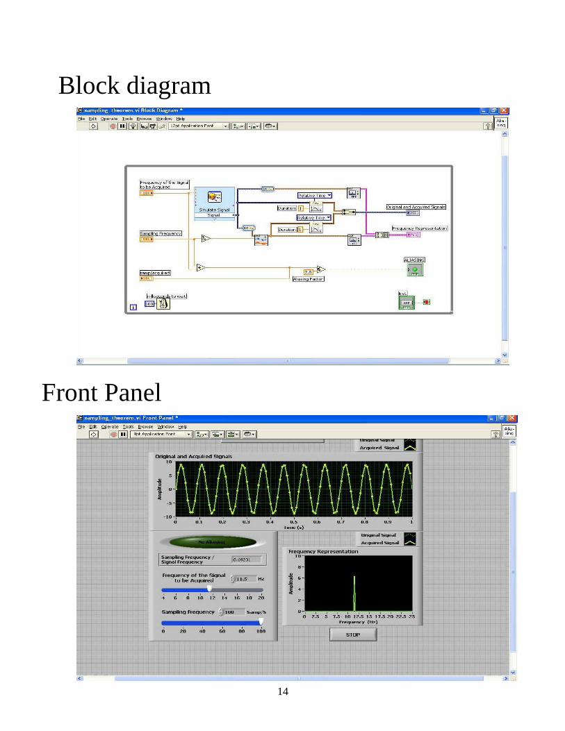
Sampling theorem (Nyquist criterion)

Theory:

The Nyquist–Shannon sampling theorem is a fundamental result in the field of information theory,

in particular telecommunications and signal processing. The theorem is commonly called the

Shannon sampling theorem. It is often referred to as simply the sampling theorem sampling is the

process of converting a signal (for example, a function of continuous time or space) into a numeric

sequence (a function of discrete time or space).

The theorem states that

“Exact reconstruction of a continuous-time baseband signal from its samples is possible if the signal

is bandlimited and the sampling frequency is greater than twice the signal bandwidth.”

The theorem also leads to an effective reconstruction formula.

14

Block diagram

Front Panel

15

Chapter 3

AMPLITUDE MODULATION

16

AAmmpplliittuuddee mmoodduullaattiioonn aanndd ddeemmoodduullaattiioonn

AM is a technique used in electronic communication, most commonly for transmitting information

via a radio carrier wave. AM works by varying the strength of the transmitted signal in relation to

the information being sent.

As originally developed for the electric telephone, amplitude modulation was used to add audio

information to the low-powered direct current flowing from a telephone transmitter to a receiver. As

a simplified explanation, at the transmitting end, a telephone microphone was used to vary the

strength of the transmitted current, according to the frequency and loudness of the sounds received.

Then, at the receiving end of the telephone line, the transmitted electrical current affected an

electromagnet, which strengthened and weakened in response to the strength of the current. In turn,

the electromagnet-produced vibrations in the receiver diaphragm, thus reproducing the frequency

and loudness of the sounds originally heard at the transmitter.

In contrast to the telephone, in radio communication what is modulated is a continuous wave radio

signal (carrier wave) produced by a radio transmitter. In its basic form, amplitude modulation

produces a signal with power concentrated at the carrier frequency and in two adjacent sidebands.

Each sideband is equal in bandwidth to that of the modulating signal and is a mirror image of the

other. Amplitude modulation that results in two sidebands and a carrier is often called double

sideband amplitude modulation (DSB-AM). Amplitude modulation is inefficient in terms of power

usage and much of it is wasted. At least two-thirds of the power is concentrated in the carrier signal,

which carries no useful information (beyond the fact that a signal is present); the remaining power

is split between two identical sidebands, though only one of these is needed since they contain

identical information.

To increase transmitter efficiency, the carrier can be removed (suppressed) from the AM signal.

This produces a reduced-carrier transmission or double-sideband suppressed carrier (DSBSC)

signal. A suppressed-carrier amplitude modulation scheme is three times more power-efficient than

traditional DSB-AM. If the carrier is only partially suppressed, a double-sideband reduced carrier

17

(DSBRC) signal results. DSBSC and DSBRC signals need their carrier to be regenerated (by a beat

frequency oscillator, for instance) to be demodulated using conventional techniques.

Even greater efficiency is achieved—at the expense of increased transmitter and receiver

complexity—by completely suppressing both the carrier and one of the sidebands. This is single-

sideband modulation, widely used in amateur radio due to its efficient use of both power and

bandwidth.

A simple form of AM often used for digital communications is on-off keying, a type of amplitude-

shift keying by which binary data is represented as the presence or absence of a carrier wave. This is

commonly used at radio frequencies to transmit Morse code, referred to as continuous wave (CW)

operation.

As with other modulation indices, in AM, this quantity, also called modulation depth, indicates by

how much the modulated variable varies around its 'original' level. For AM, it relates to the

variations in the carrier amplitude and is defined as:

18

Block diagram

Front Panel

19

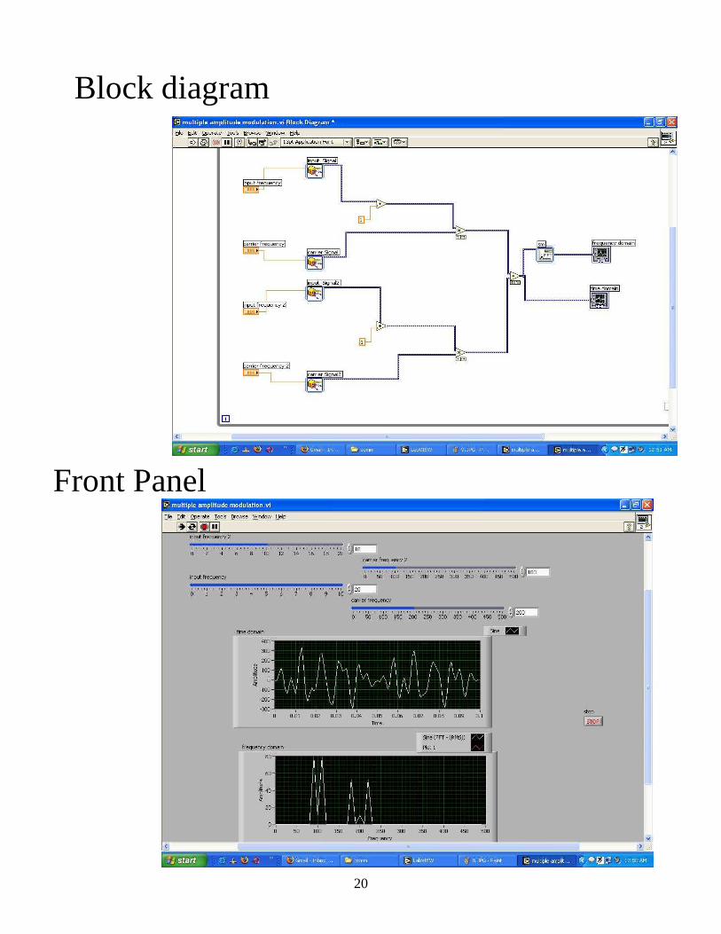
MMuullttiippllee aammpplliittuuddee mmoodduullaattiioonn

Theory:

In case of multiple amplitude modulation we use one carrier signal but we use more than one

modulating signals which result in the modulation of several input signals with the same carrier

signal. it is typically useful in multi signal environments

20

Block diagram

Front Panel

21

DSB-SC generation

Theory:

Double-sideband suppressed-carrier transmission (DSB-SC): transmission in which (a)

frequencies produced by amplitude modulation are symmetrically spaced above and below the

carrier frequency and (b) the carrier level is reduced to the lowest practical level, ideally completely

suppressed.

In the double-sideband suppressed-carrier transmission (DSB-SC) modulation, unlike AM, the

wave carrier is not transmitted; thus, a great percentage of power that is dedicated to it is distributed

between the sidebands, which implies an increase of the cover in DSB-SC, compared to AM, for the

same power used.

DSB-SC transmission is a special case of Double-sideband reduced carrier transmission. The name

"suppressed carrier" comes about because the carrier signal component is suppressed -- it does not

appear (theoretically) in the output signal. This is apparent when the spectra of the output signal is

viewed.

22

Block diagram

Front Panel

23

SSB amplitude modulation

Theory:

Single-sideband modulation (SSB) is a refinement of amplitude modulation that more efficiently

uses electrical power and bandwidth. It is closely related to vestigial sideband modulation (VSB).

Amplitude modulation produces a modulated output signal that has twice the bandwidth of the

original baseband signal. Single-sideband modulation avoids this bandwidth doubling, and the

power wasted on a carrier, at the cost of somewhat increased device complexity. The front end of an

SSB receiver is similar to that of an AM or FM receiver, consisting of a super heterodyne RF front

end that produces a frequency-shifted version of the radio frequency (RF) signal within a standard

intermediate frequency (IF) band.

To recover the original signal from the IF SSB signal, the single sideband must be frequency-shifted

down to its original range of baseband frequencies, by using a product detector, which mixes it with

the output of a beat frequency oscillator (BFO). In other words, it is just another stage of

heterodyning.

24

Block diagram

Front Panel

25

Chapter 4

PULSE MODULATION

26

PULSE AMPLITUDE MODULATION :

Theory:

Pulse-amplitude modulation, acronym PAM, is a form of signal modulation where the message

information is encoded in the amplitude of a series of signal pulses.

Detecting the amplitude level of the carrier at every symbol period performs demodulation.

Pulse-amplitude modulation is now rarely used, having been largely superseded by pulse-code

modulation, and, more recently, by pulse-position modulation.

In particular, all telephone modems faster than 300 bit/s use quadrature amplitude modulation

(QAM). (QAM uses a two-dimensional constellation).

27

Block diagram

Front Panel

28

Pulse width modulation (PWM)

Theory:

Pulse-width modulation (PWM) of a signal or power source involves the modulation of its duty

cycle, to either convey information over a communications channel or control the amount of power

sent to a load.

Pulse-width modulation uses a square wave whose duty cycle is modulated resulting in the variation

of the average value of the waveform. If we consider a square waveform f(t) with a low value ymin, a

high value ymax and a duty cycle D (see figure 1), the average value of the waveform is given by:

The simplest way to generate a PWM signal is the interceptive method, which requires only a saw

tooth, or a triangle waveform (easily generated using a simple oscillator) and a comparator. When

the value of the reference signal is more than the modulation waveform, the PWM signal is in the

high state, otherwise it is in the low state.

29

Block diagram

Front Panel

30

Pulse position modulation (PPM)

Theory:

Pulse-position modulation is a form of signal modulation in which M message bits are encoded by

transmitting a single pulse in one of 2M possible time-shifts. This is repeated every T seconds, such

that the transmitted bit rate is M/T bits per second. It is primarily useful for optical communications

systems, where there tends to be little or no multipath interference.

One of the key difficulties of implementing this technique is that the receiver must be properly

synchronized to align the local clock with the beginning of each symbol. Therefore, it is often

implemented differentially as Differential Pulse-position modulation, whereby each pulse position

is encoded relative to the previous pulse, such that the receiver must only measure the difference in

the arrival time of successive pulses. It is possible to limit the propagation of errors to adjacent

symbols, so that an error in measuring the differential delay of one pulse will affect only two

symbols, instead of causing all successive measurements to be incorrect.

Aside from the issues regarding receiver synchronization, the key disadvantage of PPM is that it is

inherently sensitive to multipath interference that arises in channels with frequency-selective fading,

whereby the receiver's signal contains one or more echoes of each transmitted pulse. Since the

information is encoded in the time of arrival (either differentially, or relative to a common clock),

the presence of one or more echoes can make it extremely difficult, if not impossible, to accurately

determine the correct pulse position corresponding to the transmitted pulse

31

Block diagram

Front Panel

32

Chapter 5

ADVANCED COMMUNCIATION TECHNIQUES

33

Time division multiplexing(TDM)

Theory:

Time-division multiplexing (TDM) is a type of digital or (rarely) analog multiplexing in which two

or more signals or bit streams are transferred apparently simultaneously as sub-channels in one

communication channel, but physically are taking turns on the channel. The time domain is divided

into several recurrent timeslots of fixed length, one for each sub-channel. A sample, byte or data

block of sub-channel 1 is transmitted during timeslot 1, sub-channel 2 during timeslot 2, etc. One

TDM frame consists of one timeslot per sub-channel. After the last sub-channel the cycle starts all

over again with a new frame, starting with the second sample, byte or data block from sub-channel

1, etc.

In its primary form, TDM is used for circuit mode communication with a fixed number of channels

and constant bandwidth per channel.

What distinguishes time-division multiplexing from statistical multiplexing such as packet mode

communication (also known as statistical time-domain multiplexing, see below) is that the time-

slots are recurrent in a fixed order and pre-allocated to the channels, rather than scheduled on a

packet-by-packet basis. Statistical time-domain multiplexing resembles, but should not be

considered as, time division multiplexing.

In dynamic TDMA, a scheduling algorithm dynamically reserves a variable number of timeslots in

each frame to variable bit-rate data streams, based on the traffic demand of each data stream.

34

Block diagram

35

Front Panel

36

Frequency division multiplexing (FDM)

Theory:

Frequency-division multiplexing (FDM) is a form of signal multiplexing where multiple baseband

signals are modulated on different frequency carrier waves and added together to create a composite

signal.

FDM can also be used to combine multiple signals before final modulation onto a carrier wave. In

this case the carrier signals are referred to as subcarriers: an example is stereo FM transmission,

where a 38 kHz subcarrier is used to separate the left-right difference signal from the central left-

right sum channel, prior to the frequency modulation of the composite signal. A Television channel

is divided into subcarrier frequencies for video, color, and audio. DSL also uses different

frequencies for voice and for upstream and downstream data transmission on the same conductors.

Where frequency division multiplexing is used as to allow multiple users to share a physical

communications channel, it is called frequency-division multiple access (FDMA).

FDMA is the traditional way of separating radio signals from different transmitters.

In the 1860 and 70s, several inventors attempted FDM under the names of Acoustic telegraphy and

Harmonic telegraphy. Practical FDM was only achieved in the electronic age. Meanwhile their

efforts led to an elementary understanding of electro acoustic technology, resulting in the invention

of the telephone.

37

Block diagram

Front Panel

38

Amplitude shift keying (ASK)

Theory:

Amplitude-shift keying (ASK) is a form of modulation that represents digital data as variations in

the amplitude of a carrier wave.

The amplitude of an analog carrier signal varies in accordance with the bit stream (modulating

signal), keeping frequency and phase constant. The level of amplitude can be used to represent

binary logic 0s and 1s. We can think of a carrier signal as an ON or OFF switch. In the modulated

signal, logic 0 is represented by the absence of a carrier, thus giving OFF/ON keying operation and

hence the name given.

Like AM, ASK is also linear and sensitive to atmospheric noise, distortions, propagation conditions

on different routes in PSTN, etc. Both ASK modulation and demodulation processes are relatively

inexpensive. The ASK technique is also commonly used to transmit digital data over optical fiber.

For LED transmitters, a short pulse of light and binary 0 represents binary 1 by the absence of light.

Laser transmitters normally have a fixed "bias" current that causes the device to emit a low light

level. This low level represents binary 0, while a higher-amplitude light wave represents binary 1.

39

Block diagram

Front Panel

40

REFERENCES

1. Learning with LabVIEW 7TM EXPRESS

- Robert H. Bishop

2. "Product Activation FAQ", National Instruments.

3. "Building a Stand-Alone Application", National Instruments.

4. "Using the Lab VIEW Run-Time Engine", National Instruments.

5. Internet references:

http://www.ni.com/events/tutorials/campus.htm

http://forums.ni.com/

http://zone.ni.com/devzone/fn/p/sn/n15:EXAMPLE

http://www.wikipedia.com/