application of wave, mechanics theory d … · application of wave, mechanics theory to flu d...
TRANSCRIPT

Technical Report. 1-
APPLICATION OF WAVE, MECHANICS THEORY
TO FLU D DYNAMICS PROBLEMS -FUNDAMENTALS
(NASA-CR-14084) APPLICATION OF WAVE N75-12228
I-
MECHANICS TEORY TO FLUID DYNAMICS
-j :
PROBLEMS: FUNDAMENTALS (Michigan StateUniv.) 206 p HC $7.25 CSCL 20D Unclas
G3/34 02833
Division of Engineering ResearchMICHIGQAN STATE IUNIVERSITYEast Lansing, MichiganOctober 30, 1974
- ""-.
https://ntrs.nasa.gov/search.jsp?R=19750004156 2018-08-19T23:43:50+00:00Z

Technical Report No. 1NGR-23-004-085NASA Langley Research CenterHampton, Virginia 23365
APPLICATION OF WAVE MECHANICS THEORY
TO FLUID DYNAMICS PROBLEMS-- FUNDAMENTALS
prepared by:
M. Z. v. Krzywoblocki, Principal InvestigatorJudity C. Donnelly, Research Assistant (up to March 15, 1973)Robert M. Johnson, Computer Programmer (up to June 30, 1973)Sidney Katz, Computer Programmer (up to June 30, 1973)S. Kanya, Computer Programmer (up to September, 1973)D. Wierenga, Computer Programmer (up to September, 1973)David Keenan, Computer Programmer (up to June 30, 1974)John Dingman, Computer Programmer (up to June 30, 1974)
Division of Engineering ResearchMICHIGAN STATE UNIVERSITYEast Lansing, MichiganOctober 30, 1974

ACKNOWLEDGEMENT
Appreciation is expressed to NASA Langley Research Center,
Hampton, Virginia, who sponsored the research under Grant NGR-23-
004-085. The work was done in the College of Engineering, Michigan
State University, East Lansing, Michigan, and the results are the
property of the U. S. Government. All rights for Technical Reports 1,
2 and 3 are reserved and may not be reproduced without permission
of the U. S. Government and/or the author.
Special thanks are due to Dr. John Ward, previously NASA
Langley Research Center, for continuous moral support.

TABLE OF CONTENTS
Page
Introduction .................. .... 1
1. Fundamental Considerations Relating Wave Mechanics(Microscopic) to Fluid Dynamics (Macroscopic) . ..... 1
1. 1. The Mathematical and Physical Features . ........ 1
1. 2. Elementary Considerations Relating to the SubmacroscopicNature . . . . . . . . . . . . . . . . . . . . . . . . 8
1.3. Transition Point . . . . . . . . . . . . . . . . .. .. . 13
1.4. General Stress-Strain System in Macroscopic ViscousFluids . . . . . . . . . . . . . . . . . . . . . ... 14
1. 5. Experimental Coefficients. ............ .. . . 18
2. Fundamental Aspects of Wave Mechanics Theory . . . . . 18
2. 1. Schroedinger Equation and its Characteristic Properties . 18
2. 2. Scale Magnification Factors ... . . . . . . . . . . . . . 21
2.3. Resonance.. . . . .. . . . . .. . . . . . . . . . . . . 31
3. Laminarity of the Flow ........... ..... 34
3. 1. Presentation of the Problem . . ....... .... . . . 34
3. 2. Curl, Vortex Frequency, and Radius of the Vortex. . . . . 36
3. 3.. Stream Function and Velocity Potential Function . ..... 44
3.4. Streamlines . . . . . . . . . .. . . . . . . . . . .. 48
4. Velocity Potential . . . . . .. .. . . . . .. .. 49
4. 1. Velocity Potential Function: Quasi-Potential Function . 49
4. 2. Velocity Potential Function: Complex Variable Function. 67
4.3. Diabatic Flow . ................ ..... 71
5. Special Mathematical Considerations . . . . . . ....... 75
5. 1. Some Characteristic Properties of Linear Systems . . .. 75
5.2. ENSS Operators . . . . . . . . . . . . .... . ... 84
5. 3. Elements of Probability Calculus . . . . . . ... . . 101
5.4. Field Theory (Explanation) . . . . . . . . . . . . . . . 104
6. Disturbances in Fluids . . . ......... . ... . .. . 105
6. 1. Geometrical and Mechanical Aspects of Disturbances(Turbulence - A Special Case) . . . . . . . . .... . 105
6.2. Gradient Plus Curl ......... ...... .. . .112
6. 3. Operations on the Disturbed Flow . . . . . ... . . . . 120
iii

Page
6.4. Disturbance in the Thermal Boundary Layer. . . . . . . 133
6.5. Computer - Analyzed - Geometrical - GraphicalPlottering - Step-by-Step - Successive - Iterative -Approximation - Quantum - Theoretic - Method . . . . . 137
7. Introductory Elements of the Bifurcation Theory ... . . 143
7. 1. Mathematical Elements of the Bifurcation Theory . . . 143
7.2. Application of the Bifurcation Theory . . . . . . . . . 150
7.3. List of References to Section 7. . . . . . . . . . . . . 154
8. Laminar Flow .. . . . . . .. . . . . . . . . . . . 154
8. 1. Macroscopic Laminar Flow . ..... . . . . . . . . . 154
8.2. Association Between Two Domains: Wave Mechanics(Microscopic) and Classical, Deterministic(Macroscopic) Fluid Dynamics . . . . .. . . . . . .... 156
8.3. Step-by-Step Successive Iterative Method . . . . . . . . 158
8.4. Diabatic Flow . . .. . . . . . . . ... .. . . .. . 160
8.5. True Nature of the Laminar Flow .. . . . . . . . . . 161
8.6. Elementary Notions of Particle Kinetics . . . . . . . . 167
8.7. Possible Degrees of Freedom . .... . . . . . . . . 170
9. Other Possible Forms of Wave Equation and Physio-
logical Aspects. . . . .. . . . . .. . . . ..... 175
9.1. Schroedinger Equation ..... .. .. . . . . . . . . . . 175
9.2. Physiological Aspects in Fluid Dynamics (Turbulence inParticular) and True Role of Reynolds Number . . . . . 180
9.3. Description of Plots.. .. . .... .... ...... . 181
9.4. Concluding Remarks .. . . . . . . . . . . . . . . . 183
10. Modern Task of Computer . ............. . 183
10. 1. New Tool for Aerodynamists . ............. 183
10.2. Present Research as a Part of Modern Tool ofAerodynamics . . . . . . . . . . . . .. . . . . . . 185
PRECEDING PAGE BLANK NOT FILME
v

INTRODUCTION
The primary goal of this report is to explain the application of
the basic formalistic elements of wave mechanics theory, usually con-
sidered as being a proper tool describing the physical phenomena on the
microscopic level, to fluid dynamics of gases and liquids, usually con-
sidered as being a proper tool to describe the physical phenomena on
the macroscopic level (visually observable). The practical advantages
of relating the two fields (wave mechanics and fluid mechanics) through
the use of the Schroedinger equation will constitute the approach to thi s
relationship.
1. FUNDAMENTAL CONSIDERATIONS RELATING WAVE MECHANICS
(MICROSCOPIC) TO FLUID DYNAMICS (MACROSCOPIC)
1. 1. The Mathematical and Physical Features
Before a discussion and description of many important, particular
aspects of the association of wave mechanics theory to fluid dynamics,
a few general remarks are in order. Some particular aspects are
immediately obvious from the statement of the general goal:
(a) Considerations of a mathematical nature: As a general
(unwritten) rule, the majority of fields in the domain of the
mechanics of solids and fluids (liquids and gases) are governed
by systems of equations of a nonlinear (sometimes highly
nonlinear) nature (Newtonian mechanics). The wave mechanics
equation of Schroedinger is a linear equation. A set of
Schroedinger equations can be added (summed) or subtracted;
their solutions can be multiplied by a constant or a set of con-
stants; this is one of the advantages of linear partial differen-
tial equations (the class of equations to which the Schroedinger
wave equation belongs). The highly nonlinear terms which
appear in the classical equations of Euler and Navier-Stokes
(based upon Newtonian mechanics) cannot be compared with
the advantages of linear equations. As is well known, there
does not exist an exact or a correct definition of the non-
linear aspects of partial differential equations. There exists
no knowledge of the characteristic properties and behavior
1

of nonlinear partial differential equations (much less of their
solutions).
All characteristic features of the linear, as contrasted
to the nonlinear partial differential equations, are basic
when dealing with equations which describe the important
characteristic, physical aspects and physical behavior of
liquid or gaseous media. In physical results, more often
than not, there arises the necessity of adding the results of
the numerical calculations or of multiplying them by a con-
stant. These are only a few examples for illustrative pur-
poses.
(b) Characteristics of a physical nature: The approach in deter-
mining the behavior and fundamental characteristics of liquids
and gases of macroscopic fluid dynamics is based, among
others, upon the notion of density. This means that the
smallest amount of the medium which can be considered is3
the amount of mass per unit volume, e.g. cm . The physical
considerations are adjusted to this concept and the macro-
scopic measurements are adjusted to this concept as well.
However, in reality, the smallest amount of fluid which can
be put in motion due to disturbances which may be introduced
into the medium may be smaller (even much smaller) than
a cubic centimeter. These and similar problems are not
simple when treated exclusively in the domain of macro-
scopic fluid dynamics; but their solutions become simpler
when treated by means of wave mechanics theory. In the
Schroedinger equation, the mass "m" of the element in ques-
tion refers basically to the mass of the electron(m = 0. 9107 x
10-27 gram or m = 0. 911 x 10 gram, (F. K. Richtmyer and
E. H. Kennard, Introduction to Modern Physics, McGraw-
Hill Book Company, Inc. , 1947, pp. 85 and 216). In practice,
one may use the concept of the "cluster" of electrons or the
concept of the cluster of molecules guided by the electron
under consideration as their "leader" in place of "m" in the
Schroedinger equation. The cluster may have a mass with
2

reference to the volume less than that of a cubic centimeter.
It should obviously refer to a volume corresponding to the
mass greater than that of an electron but smaller than the
mass of the medium in question with reference to a cubic
centimeter. As a matter of fact, the investigator is of the
impression that during the phenomenon of perturbations due
to disturbances introduced in some cases into a medium, it
is not the mass of the medium with reference to the cubic
centimeter which takes part in disturbed motion, but rather
the mass with reference to the volume smaller than that of
a cubic centimeter. This conjecture, based upon visual
observations of photographs of disturbed media, requires
verification by tests and experimental measurements. The
concept of the mass of the medium in question obviously
appears in the final calculated or tested results after the
mean values are calculated and included into the numerical
scheme. The proposition of Madelung (1926) allows one to
deal with the wave equation of Schroedinger.
The approach to fluid dynamics based upon the wave
mechanics equation of Schroedinger allows one to take into
account the mass of the fluid with reference to a volume,
which is smaller than that of a cubic centimeter. Consequently,
the Schroedinger equation allows one to deal with the pheno-
mena of flow on the scale above the microscopic level (electron
level) but below the fully macroscopic level (the level which
can be tested by the use of macroscopic instrumentation --
classical, deterministic fluid dynamics). All the remarks
made above refer to the state of the fluid above that of super-
fluidity. This means that the state of the fluid is above the
phase transition phenomenon and above the X - point (nor-
mally at a temperature much above absolute zero).
One additional remark is appropriate. The following
description is used with reference to some physical phenomena:
nuclear level, nuclear phenomena, extension of quantum
theory to the domain of nuclear dimensions, and the like.
3

A question may arise as to the kind of particles the work
"nuclear" should or might refer to. Since it is desired to
avoid a presentation of "Theoretical Physics," the reader is
asked to turn to the appropriate literature with regard to
these problems of the nomenclature. The most important
matter in the presentation of this quantum approach is the
"understanding" of the new concept of the new idea.
For the purposes presented in this report it is sufficient to men-
tion that a matter (a solid or a fluid, liquid or gas) (or briefly a sub-
stance) is built of molecules. A molecule, in turn, is built of atoms
(example: molecule of water vapor is a cluster of two hydrogen atoms
and one oxygen atom.) The smaller entities than an atom are: proton,
neutron, electron, meson (see O. M. Stewart, Physics, Ginn and
Company, 1944, p. 189). The electron has a negative charge and a mass
of = 0. 917 x 10 - 27 gram (F. K. Richtmayer and E. H. Kennard, Intro-
duction to Modern Physics, McGraw-Hill Comp., 1947, p. 85). One of
the fundamental equations describing the behavior of small entities in
various physical phenomena is Schroedinger wave equation (1926). This
will be used below by the writer. The element appearing in Schroedinger
equation is an electron. The elements heavier than an electron are built
from a combination of protons and neutrons. Consequently, in the approach,
used below by the writer, the notion of an electron is generalized to the
notion of a cluster of protons, neutrons , atoms and molecules gathered
around the electron in question and guided by it. In such a way, the
author is allowed to apply the Schroedinger equation to any mass element
which ever it may appear in the physical phenomenon in question, start-
ing from the electron on one side and ending with classical, macroscopic
concept of density on the other.
In previous centuries only one approach was used in the descrip-
tion and application of the theory of fluid dynamics; i. e., the approach
based upon the Newtonian mechanics. This approach was, and still
remains very powerful. From the mathematical point of view, it is based
upon the deterministic mathematics; i. e. , the theory of functions (in
particular, theory of analytic functions). Many problems in the past were
solved using this approach which gave good agreement with experimental
4

data. The fundamental equations used in these approaches were Euler's
equation, Navier-Stokes equation and equations based upon Boltzmann
kinetic theory.
The beginning of the twentieth century witnessed the appearance
of another approach to describe the dynamic-mechanical problems; viz,
the quantum approach. This approach uses probabilistic mathematics
as its tool, and is primarily used to describe phenomena which are so
small (such as the motions of an electron), that they cannot be described
by the macroscopic, deterministic equations. For a number of years
science tried to make a definite distinction between the fields of science
operating in the small (molecular) and in the large (macroscopic)
phenomena. The first was referred to as physics, and the second as
mechanics (of solids, of fluids, of gases, etc. ). Over the course of
years it became obvious that the phenomena in the "small" influenced
the phenomena in the "large",. and vice versa, and that distinctions
above should be abolished. Thus physics entered the field of the
mechanics of solids, thereby explaining such phenomena as "superfluidity. "
This, however, is not yet sufficient since there are many practical
phenomena, such as the interaction of the mechanics of fluids or gases
with electromagnetic wave propagation, whi ch need explanation of the
interaction phase.
Such an approach can belong to both the mechanics of electro-
magnetic wave propagation and to the mechanics of fluids. There are
some instances where immediate application to both electromagnetic
wave propagation and turbulent fluid behavior is in order. Nature does
not and cannot care about any such distinction between phenomena. All
such phenomena are "natural" phenomena, and distinctions were made by
scientists alone. This enables the scientist to provide an easier descrip-
tion so that others may better understand.
The results of the "interference" and of the "interaction" described
previously appear in the phenomenon of "refractivity", which is very
important in considering the problem of wave propagation through fluid
media (radio waves). The analytical approach to the problem of refrac-
tivity can be theoretically approached from the viewpoint of Newtonian
fluid mechanics or from the viewpoint of electromagnetic wave propagation
5

(quantum). The problem is important to physicists, applied mathemati-
cians, and engineers who are engaged in the field of propagation. In the
past the first approach produced useful results, but in the last twenty or
thirty years it has become obvious that the approach from the quantum
side can possibly give even better results. Thus, in the last decades the
American and Soviet schools of physics developed the so-called "methods
of quantum field theory in statistical physics." These became very power-
ful in explaining such phenomena as superconductivity, theory of the Fermi
liquid, electromagnetic radiation in absorbing media, refractivity,, etc.
Since the methods are relatively new, a decision has not as yet been
reached as to which particular field is the appropriate one for having
them included; whether classical physics, modern physics, applied
physics, theoretical mechanics, applied mechanics, fundamental mathe-
matics, applied mathematics, physico-mathematics, or some new spe-
cial field that might be developed.
Another question is at which university level these methods should
be given to students -- first year graduate students, second year graduate
students, or to only Ph. D. candidates in their last year of work -- and
should exposure be in regular courses or seminars only. It is clear
that the above concepts cannot be treated as rules but only as propositions
and they are not general propositions, but are such that they should be
applied only in special cases, namely to cases in whi ch they might give
better practical results than those presently obtainable. It is generally
known that the methods of quantum field theory in statistical physics have
recently become (in some fields and for some problems) the strongest
methods presently available to scientists.
As mentioned above, the purpose of the present work is a two-
fold one: formalism of the application of the wave mechanics to
macroscopic fluid dynamics and a discussion of practical advantages of
the association of wave mechanics with macroscopic fluid dynamics. The
first step towards this goal will involve laminar flow having visible
streamlines. Disturbances in the form of a curl of the velocity vector
are introduced into this system. Due to the fact that the entire flow
system is described in terms of wave functions and by means of the
Schroedinger equation, the above disturbances can be geometrically
6

added (superimposed) upon the laminar flow system.
An analogous situation occurs in the phenomenon of turbulence.
Truly speaking, in the case of turbulence, there may also appear the
phenomenon of resonance which is an item to be discussed separately.
In order to avoid confusion in the nomenclature, the words "disturbed
flow" will be used to describe the status of the flow system in which
turbulence may appear, as well as any other kind of mechanical or
thermal disturbance. As an example of a disturbed flow system, tur-
bulent flow, turbulence, theories of turbulence, classical theories of
turbulence, and so on, will occasionally be cited.
The proposition of applying wave mechanics theory to turbulence
has an advantage over the classical statistical theories of turbulence
which use highly nonlinear (unsolvable) classical, deterministic Navier-
Stoker equations; the wave mechanics theory uses Schroedinger equation
(or a system of linear equations and solutions). In the classical statis-
tical theories, the concept of mean values is defined according to Rey-
nold's rules (1883), which refer to macroscopic observations in gaseous
and liquid flows. These have been accepted by subsequent investigators.
In wave mechanics theory the assumption that turbulence is a natural
phenomenon, which becomes observable at Recr but exists above the
transition point, is the important factor which enables one to apply
this "natural" approach to turbulence. All systems which oscillate
"are quantized, whether they are material oscillators, sound waves, or
electromagnetic waves. " In quantum theory, the mean values are defined
without ambiguity. In classical statistical theories, mathematics (namely
algebra) could not adequately solve the question of Renold's mean values
(see the works of G. Birkhoff, J. Kampe' de Fe'riet, and others). In
wave mechanics theory the propositions of the mean values in the pro-
bability calculus are generally accepted and successful. In classical
statistical theory, the existing theories of turbulence are not too success-
ful, whereas in the wave mechanics approach it will be demonstrated that
wave mechanics can be used to attack the problem of "self-excitable"
turbulence (C. A. T. ). In the classical statistical approach the use of
Navier-Stokes equations violates the fundamental theorem and proof of
John von Neumann on "hidden variables. " In classical statistical theory,
7

the notion of correlation functions between two (or more) points was intro-
duced, while in wave mechanics the same can be done with the use of the
wave function. In classical statistics the trend is to solve the determin-
istic, causal (or stochastic) system (nonlinear) in a classical manner;
in wave mechanics the wave functions and equations give only the pro-
babilistic value, but in the realistic (classical) limit the observation is
so rough that the difference between "the probable and actual behavior
is never detected. " In classical statistics seldom reference is made to
the phenomenon of resonance. In wave mechanics the writer calls atten-
tion to this phenomenon in C.A.T. , and it is possible that the phenome-
nona appear in several other kinds of disturbances as well. Actually,
a "laminar" flow does not exist. That which is referred to as macro-
scopically and observable laminar flow is, in reality, microscopically
turbulent flow. The value of the observable property of laminar flow
is actually the mean value of the property of a submacroscopic (or
microscopic) turbulent flow. In reality, it was W. Heisenberg in 1948
who stated that fluid dynamicists should give greater research emphasis
to laminar flow rather than to turbulent flow.
1. 2. Elementary Considerations Relating to the Submacroscopic Nature
In recent years, remarkable success has been achieved in many
domains of statistical physics due to the extensive use of methods based
upon the quantum field theory. Statistical physics studies the behavior
of systems consisting of a very large number of particles. In the last
analysis, the macroscopic properties of liquids and gases are due to
microscopic interactions between the particles making up the system.
The overall macroscopic characteristics are determined by certain
average properties of the system. The macroscopic state of a system
is specified by the pressure P, the temperature T, and the average
number of particles N in the system. A closed system of N particles is
characterized by its energy levels. Due to the wavy structure of matter,
the smallest elements of the medium are subject to vibrations and systems are
described as a superposition of monochromatic plane waves. Each
wave is characterized by a wave vector, k and consists of several branches,
W0 (k), the total number of branches equal to 3r, where r is the number
of particles belonging to the unit volume of the medium. For small
8
momenta, the three (accoustic) branches are characterized by the fact
that the frequency depends linearly on the wave vector:
ws(k) = u s , us = velocity of sound. (. 2.1)
Unless the contrary is explicitly 'stated, a system of units in
which both Planck's constant and the velocity of light equal 1 will be used.
From a knowledge of the frequency spectrum, the energy levels, and the
coordinates, one can calculate, in principle, the thermodynamic and
kinetic characteristics of the vibrating elements. Another model can be
obtained by applying the "correspondence principle, " which states that
every plane wave corresponds to a set of moving particles (called phonons)
with momentum determined by the wave vector k and energy determined
by the frequency ws(k). This leads to an expression for the energy levels
of the system which is analogous to that for an ideal gas. With n. inter-
preted as the number of phonons in the state i = (k, s) where n. covers
the range of all integers, including zero, the energy spectrum of a system
is given by the formula:
3N
E = i (n + 1/2) (Bose statistics)
(1. 2. Z)
The phonons and neutral gases obey Bose statistics.
Since this work is restricted solely to the question of the applica-
tion of wave mechanics to macroscopic fluid dynamics, it will be impos-
sible to present many details of the fundamental nature of wave or quan-
tum mechanics. Consequently, for more details on the fundamentals of
wave or quantum mechanics and of possible models of the nature of quan-
tum, the reader should refer to the appropriate literature.
Two more items which are pertinent to the general considerations
of the physical and geometrical nature of the association of wave mechanics
with the macroscopic fluid dynamics are phase transition and the stress-
strain deformation system. As is seen from the introductory remarks,
the general field of fluid dynamics (liquids and gases) can be divided
roughly into two subfields: (a) fluids (both liquids and gases) which obey
the laws of Newtonian (1642 - 1727) mechanics, and may be described
9

with sufficient accuracy by means of the language of classical, deter-
ministic Newtonian mechanics, and (b) fluids (both liquids and gases)
in which the physical behavior demonstrates very clearly a lack of
complete determinism of elementary processes. This compels science
to accept far-reaching changes in the general concepts concerning the
fundamental nature of matter and of energy. In the description of the
phenomena in these kinds of fluids one has to use the language of modern
mechanics, wave and quantum mechanics, originated by Bohr (1913).
In particular, when describing the behavior of some fluids at low tempera-
tures, one must use the language of modern mechanics. For example,
the research was initiated with the very elementary concept of super-
fluidity (or superfluid fluids) where the fluids in question belong to the
class of Bose statistics fluids (liquids and gases). The most interesting
property of a Bose liquid is the property of "superfluidity," i. e. , the
possibility of flowing through capillary tubes without friction (Landau,
1941) (liquid helium).
Consider a Bose liquid at absolute zero, flowing with velocity v
in a capillary. In the coordinate system fixed with respect to the liquid,
the liquid is at rest and the capillary moves with velocity -v. As a result
of friction between the liquid and the wall of the capillary, the liquid
begins to be "carried along" by the wall. This means that the liquid
begins to have non zero energy and momentum, which is possible only
if elementary excitations appear in the liquid. As soon as a single such
excitation appears, the liquid acquires momentum p and energy E(p).
Now, suppose one is to go back to the coordinate system fixed
with respect to the capillary. In this system, the energy of the liquid
equals:2
E + p * v + 1/2 My (1.2.3)
Thus, the appearance of an excitation changes the energy by an amount
E + p I v. In order for such an excitation to appear, the change in energy
must be negative, i. e.,
E + p v < 0. (1. 2.4)
The quantity E + p * v takes its minimum value when p and v have opposite
directions. Thus, in any case, one must have:
10

E - p < 0 or v> E/p. (1.2. 5)
See: (A. A. Abrikosov, L. P. Gorkov, J. E. Dzyloshinski , Methods of
Quantum Field Theory in Statistical Physics, 1963, p. 11).
This means that in order for it to be possible for any excitations to
appear in the fluid, the velocity must satisfy the condition:
v >(E/P)min. (1. 2. 6)
The minimum value of E/p corresponds to the point of the curve E(p) where:
dE E (1. 2. 7)dp p'
i. e. , the point where a line drawn from the origin of coordinates is tan-
gent to the curve E(p). Thus, superfluid flow can occur only in the case
where the velocity of the liquid is less than the velocity of the elementary
excitation at the points satisfying the condition (1. 2. 7). It is recalled
that dE/dp is the velocity of the elementary excitation. For every Bose
liquid, these always exists at least one point where the condition (1. 2. 7)
is satisfied: namely, the origin of coordinates P = 0. Since for values
of p near zero, the excitations move with the velocity of sound, the
superfluidity condition is certainly not satisfied for flow velocities
exceeding the velocity of sound u.
Thus, one obtains the following general picture of the motion of
a Bose liquid when the velocity is such that the superfluidity condition
holds. First, the temperature T = 0 (absolute zero) is considered. If
the liquid is initially in the ground state, i. e. , if it contains no elemen-
tary excitations, then no excitations can appear later and the motion
is superfluid. For T / 0, the picture essentially changes in such a way
that the fluid contains excitations whose number is determined by the
appropriate statistical formulas. Although new excitations cannot appear,
nothing, as noted above, can prevent the excitations already present from
colliding with the walls, thereby exchanging momentum with the walls.
Only a part of the mass of the liquid participates in this viscous motion.
The remaining part of the mass of the liquid moves as before, with no
friction between it and the walls or between it and the part of the fluid
participating in the viscous flow. Thus, at T / 0, a Bose liquid represents
a kind of mixture of two liquids, one which is "superfluid" and the other
which is "normal", moving with no friction between them.
11

Of course, in reality no such separation occurs, and there are
simply two motions in the liquid, each of which has its own effective
mass or density. First, there is the "normal" density; this is denoted
by pn. The remaining part of the density of the fluid, denoted by ps'corresponds to superfluid motion, and hence:
P = Pn + Ps (1. 2. 8)
Let vn denote the macroscopic velocity of the gas of excitations,
and let v denote the velocity of the superfluid liquid. Then the velocity
v has the following basic property: If the Bose liquid is put in a cylinder
and the cylinder rotates about its axis, the normal part is "carried along"
by the walls of the cylinder and the liquid itself begins to rotate. On the
other hand, the superfluid part remains at rest, and hence does not have
to be taken into account. In other words, the motion of the superfluid
part is always irrotational, a fact which is expressed mathematically by
the condition
curl v = 0 . (1. 2. 9)
The motion of the superfluid part of the liquid imposes certain
conditions on the excitatibns. In fact, it is noted that it is precisely in
the reference system fixed with respect to the superfluid part that the
function E(p) has the form discussed above. In the rest system,
obviously one has:
E' = (p) + p " v s , (1.2.10)
where p is the momentum in the reference system fixed with respect to
the superfluid liquid. This has to be taken into account in writing the
transport equation for the excitations.
The fact that a Bose liquid contains two types of motions with
different velocities leads to a very distinctive kind of hydrodynamics
whose equations can be derived from the transport equation. The "two-
velocity hydrodynamics" of a Bose liquid differs from ordinary hydro-
dynamics in many ways. In particular, it turns out that two different
kinds of oscillations can occur in a Bose liquid, with two different
velocities of propagation. The oscillations of the first kind represent
ordinary sound, or what is called "first sound," with velocity of propa-
gation equal to u. In a sound wave of this kind, the liquid moves as a
12

whole, i. e., the normal and superfluid parts do not separate. The oscil-
lations of the second kind, the so-called "second sound," propagate with
velocity of a different value. In a wave of this kind, the oscillations of
the normal and superfluid parts of the liquid have opposite phases, and
hence the total flow vector of the liquid is:
-=py (1. 2. 11)j vnVn sV s 0.
1. 3. Transition Point
Let us now consider what can be said about the behavior of a
Bose liquid at higher temperatures, when the number of excitations in
the liquid becomes large. In this case, interaction between excitations
can no longer be neglected, and it can be assumed that this picture is
preserved for relatively high temperatures. The same applies to the
hydrodynamical equations, since they are actually consequences of
conservation laws. As the temperature increases, the normal density
Pn increases until it reaches a value equal to p. At this point, called
the %-point, a phase transition occurs in the medium. Below the transi-
tion point, superfluid motion is possible. However, above the transition
point, superfluid motion is no longer possible, and the hydrodynamics
of the Bose liquid do not differ from ordinary hydrodynamics.
In principle, the transition from pn / p to pn = p might take
place either continuously or discontinuously. It follows from an experi-
ment with helium that the normal density pn grows continuously as the
temperature increases and becomes equal to p at the X-point. Consider-
ably above the X-point, helium has no peculiarities of behavior as com-
pared with an ordinary liquid. As for the neighborhood of the X-point,
there is good reason to expect a number of essentially new properties.
The problem of the behavior of various characteristics of systems,
especially their thermodynamic properties, in the neighborhood of a
point where a phase transition occurs, remains partly unsolved at present
and represents one of the most interesting problems of the physics of
matter in the condensed state.
The macroscopic conditions may be expressed in terms of the
Navier-Stokes equations. The present task is to associate the Navier-
Stokes equations with the Schroedinger equation. In such a manner, a
13

link between a flow domain in a viscous gas and the mathematical for-
malism of the wave mechanics theory is to be constructed. The coeffi-
cients of viscosity and heat conductivity are supposed to be known and
given from the tables of standard atmosphere. It bears repetition to
state the the present approach with the use of the wave mechanics refers
to the fluid above the \-point.
All the above assumptions, which use the Navier-Stokes equations,
enables the writer to treat the fluid system as a Bose liquid above the
phase-transition X-point. Below this point the fluid is moving as a two-
phase fluid (super-fluidity and super-conductivity phenomena may be
present). Above this point the fluid dynamics of a Bose liquid does not
differ from the ordinary, classical hydrodynamics.
1.4. General Stress-Strain System in Macroscopic Viscous Fluids
The characteristic features of macroscopic fluid mechanics
which were essentially developed prior to the twentieth century to describe
the phenomena occuring in inviscid and nonheat-conducting liquids and
gases will not be discussed. It can be said that the actual development
of the field of viscous, heat-conducting liquids and gases took place in
the twentieth century. Ludwig Prandtl (Goettingen, Germany, 1904)
and his school are responsible for developing the field in a modern sense.
They based their development on previous results, particularly those of
Euler (1752 - 1755). These earlier results usually referred to inviscid,
nonheat-conducting (i. e., ideal) liquids and gases. When approaching
the theory of viscous, heat-conducting liquids and gases, one of the most
characteristic aspects which must be taken into account is the influence
of the viscosity and heat conductivity upon the dynamics of the system.
Prandtl based his approach upon the theory of solids simply because
nothing better was available at that time in either the field of solids or
fluid media.
In passing from the theory of ideal fluids to the theory of viscous
fluids, Prandtl assumed the validity of the concept of the existence of
stresses and strains in the fluid body (analogous to solids). Next, there
appeared the concept of deformable bodies in which deformations,
elongations, displacements, angular displacements, expansions, angular
deformations, and others were taken into consideration. In the case of
14

elastic solid bodies the well-known Hooke's law was used. In the case
of viscous fluids, Stokes' law of friction was substituted. These two
laws are so intimately related to one another that in deriving either one
of them, the other is simultaneously obtained. The only difference
between them is that in Hooke's law for elastic bodies, the forces which
oppose the deformation of a body are proportional to the magnitude of
the strain, whereas in Stoke' law of friction in fluids, these forces are
proportional to the rate-of-strain.
Omitting the details of this development in the post-Prandtl
era, the fact is that this proposition was and still is very successful.
It has solved many problems in applied physics and engineering. As
can be readily seen from the general outline above, the approach is
characterized by its "macroscopic" nature. A volume of the fluid in
question is treated as a solid. The internal interaction of intermolecular
forces "in the small" are taken into account by means of the coefficients
of viscosity and heat conductivity where these coefficients have to be taken
from the experimental data. To obtain better agreement between the
analysis and experimental data, two coefficients of viscosity were intro-
duced. In order to find a relation between these two coefficients of
viscosity, the kinetic theory of gases was used. This furnished the
most elementary solution -- namely zero, andallowed one to derive
the relation sought between the two coefficients of viscosity, P1 = -2/3p.
This appears to have been verified experimentally by measurements of
acoustic absorptions which have been made only for perfect monatomic
gases. Similar experiments with liquids, however, have shown that
values for the viscosity ratio differ from 2/3. It was decided to take the
Navier-Stokes equation (1822, 1826, 1845) as the fundamental equation
governing the dynamics behavior of viscous fluids.
The above outline clearly demonstrates the fact that present
day "macroscopic" fluid dynamics treats liquids and gases as large
macroscopic entities. Consequently, the phenomena which refer to
these media are also treated in a crude, macroscopic manner. No
refinements can be introduced because it is highly questionable whether
one can gain insight into the phenomena taking place inside the cubic
volume (borrowed from the theory of mechanics of solids). The numerical
15

coefficients of viscosity, first and second, are very approximate and do
not take into account the phenomena appearing inside the cubic volume,
such as inter-molecular forces, intermolecular action and reaction when
external forces are acting upon the external walls of the cubic volume.
Nothing can be said about the interference phenomena between the parti-
cular molecules or about the dynamic action of molecules upon each
other. There is not even a possibility of accomplishing this since no
equation in the macroscopic theory of fluids exists whi ch takes into
account the intermolecular action between particular molecules. However,
it is a known fact to modern physicists that phenomena in "the small" --
on the microscopic scale--influence, and to some degree may even con-
trol, phenomena in "the large"--on the macroscopic scale. From the
known phenomena in the field of fluid dynamics, the problem of turbulence,
discovered by Reynolds in 1883, was investigated by many scientists
using macroscopic fluid dynamics. The analytical system used is, of
course, the Navier-Stokes system. It can be stated now that, after many
decades of research on the problem, the macroscopic approach to tur-
bulence in viscous gases and liquids through the Navier-Stokes system,
statistical specification of the turbulent field, velocity correlation func-
tions at n-points, joint probability density function, joint probability
averages, correlation tensors, spectrum tensors, and many other items,
has not been too successful. It must be admitted, however, that some
of the results obtained were promising, but even today the problem of
turbulence remains unsolved and not well understood.
In contrast, the field of quantum fluid dynamics concerns
phenomena "in the small", the microscopic scale, as, for example,
the phenomena in liquids at low temperature such as liquid helium and
other similar, very difficult problems. Almost from the beginning of
its operation, quantum fluid dynamics proved to be very successful.
This success seems to be either partly or predominantly due to restric-
tions superimposed by methods used in the field. The problems are
usually restricted to single particles or small numbers of particles.
In using the methods of quantum field theory in statistical physics, one
may be interested in interactions between two particles (electron-phonon
interactions) and in similar interparticle phenomena. The mathematical
tool used is restricted to the Schroedinger equation for one particle
16

(electron) or to the Schroedinger representation (operator) of the changes
in time of the state of the system (density) of particles. The N particles
in question are originally in identical states, normalized by the proper
relation. In some cases, one may use the Heisenberg representation
in place of theSchroedinger representation.
The above discussion demonstrates very clearly that, in the
description of some dynamic phenomena in fluids, it may be better in
some cases to resign from the macroscopic representation (stress-
strain deformation system in a cubic volume) and to restrict one's atten-
tion to the investigation of single small particles and to the interaction
of one or two single small particles. After such small-scale phenomena
are understood, one may then investigate the phenomena in groups of
three, four, six, or ten particles, after which one can generalize the
results obtained to the "n" similar groups ( clusters) of elements in
the domain under consideration.
It can now be clearly seen that the methods of operation in both
fields are different. Quantum or wave mechanics starts from small,
microscopic elements; includes a small number of interactions between
these elements (one, two, or three), in which all are contained inside
a large, macroscopic volume; and generalizes the results obtained in
this manner to a larger number of such groups of microscopic elements
with a small number of interactions. The classical, deterministic fluid
dynamics starts from a large, macroscopic volume, containing many
small, interacting microscopic elements; disregards the interaction
phenomena between the great number of small, microscopic elements
inside the large macroscopic volume; and generalizes the results obtained
in this manner to a larger number of such macroscopic elements, always
disregarding the exact and precise calculation of the influence of the
interactions of small, microscopic elements upon the physical status
of large macroscopic elements. The coefficients of viscosity (first
and second), which supposedly should take into account the influence
of interactions between small microscopic elements upon the physical
status of large macroscopic elements, have values obtained from obsolete
macroscopic experimental test data and consequently cannot represent
precisely the results (of primary importance) of interactions between
17

microscopic elements and their influence upon the physical status of
large macroscopic elements.
1. 5. Experimental Coefficients
The previous section demonstrated that exact knowledge of the
numerical values of the physical coefficients is extremely important.
The coefficients are: first coefficient of viscosity, second coefficient
of viscosity, and coefficient of heat transfer. One should also include
here the precise values of the coefficient of kinematic viscosity. More-
over, in investigating the phenomena in the atmosphere, particularly
the upper atmosphere, one should have an excellent understanding
of the heat phenomena in the upper atmosphere, such as forced and
natural convection. Knowledge of the physical coefficients in all of the
above-mentioned phenomena is of the greatest importance. Unfortunately,
our knowledge in this respect is not only very limited, but it is obsolete.
The ratio of the two coefficients of viscosity is always given in the form-i
pl-1 = -2/3, although it is well known that this value is true in only
one particular case, a case which does not always occur in practice.
The conclusion is that more precise and more exact values of
the physical coefficients should be supplied for all the phenomena,
particularly when the variations in pressure, temperature, vapor coeffi-
cients and coefficients of viscosity due to changes in altitude have to be
taken into account. This is particularly important for the conditions con-
ductive to the phenomenon of C. A. T.
2. FUNDAMENTAL ASPECTS OF WAVE MECHANICS THEORY
2. 1. Schroedinger Equation and Its Characteristic Properties
This research omits all the explanations and details referring
to the physical characteristics of wave mechanics theory, in particular
the characteristic quantum theoretical features such as wave-particle
duality, wavy nature of matter, and so on. The description will be
limited to the formal aspects and to the formal association between wave
mechanics theory and classical, deterministic fluid dynamics.
The fundamental equation which describes wave mechanics
phenomena in the formal, mathematical language is the Schroedinger
wave equation of the form
18
V - 8 Z mh 2 - i 41wmh-B/t = 0 , (2.1.1)
where
V 2 = Laplace operator (Laplacian) in the three-dimensional
Cartesian coordinate space (x,y,z);
4, = the wave function, = 4, (x,y,z,t);
m = the mass of the electron;
h = Planck's constant = 6. 6 x 10 erg-sec.;
t = time (sec);
( = the external potential energy (function of the position of
the electron);
i =
From the formalistic point of view, the basic concepts of wave
mechanics employ probability theory as the main tool in its application
for the solution of various problems. Although not generally realized,
the treatment of wave mechanics as a field of mechanics has been receiving
increased attention during the past several decades. This is because
the results of wave mechanics, when applied to many fields of mechanics,
correspond closely with those obtained from many of the tests and experi-
ments in mechanics, Thus, it is very difficult to talk about the differences
in values obtained from numerical analysis or from experiments. As
a matter of fact, in recent years remarkable success has been achieved
in physics by the extensive use of methods borrowed from quantum field
theory.
The success of these methods is associated in some cases with
the application of "Feynman diagrams. " The basic advantage of the dia-
gram technique lies in its intuitive character. Operating with one-
particle concepts, one can use the technique to determine the structure
of any approximation and the required expressions can then be written
with the aid of correspondence rules. These new methods make it
possible not only to solve a large number of problems which do not
yield to the old formulation of the theory, but also to provide many new
relations of a general character.
From the wave equation, Equation (2. 1. 1) and using the wave
function in the form 4 = a exp (i p), with (a, j) dependant upon both
19

time and space, in 1926 Madelung obtained two equations, both real, L, I,
which denote the real and imaginary parts, R and I respectively:
L R () = + (Vf) 2 + m - (V a) a- h(8w 2m)' = 0 (2. 1. 2)
LI( ) = V (aV) + a (a2)/8t = 0 (2.1.3)
where: = - h (Zwm)
Applying the V operator to the equation (2. 1. 2) and using
U = VP (velocity vector) and
a = p (density of the medium),
Modelung obtained
/at + v(U ) + m V'- V[ V Z ah (8w m ) ] = 0, (2.1. 5)
V' (pU) + ap/at =0, (2. . 6)
V(V )2 =2[U , VU + Ux(Vx U)], (2.1.7)
where V x U = 0,
with equation (2. 1. 5) corresponding to the Euler equation of motion and
equation (2. 1. 6) to the equation of the conservation of mass (continuity).
The following interpretation of Madelung's development can be proposed:
-1 -1 -0m VD represents p f = the action of the extraneous force field,
-1 2 2 2 2 -1and a V a h (8w mI = the action of the static pressure, which is
equivalent to the term [ -S p-1 dp] in classical macroscopic fluid dyna-
mics, where p denotes the static pressure in the medium.
Equations (2. 1. 5) and (2. 1. 6) are equivalent to equation (2. 1. 1)
and represent a form of transformation of the wave equation, (equation
(2. 1. 1),), into two parts, one real and the other one imaginary. They are
obtained by elementary operations, such as the gradient operator V,
the decomposition of the Schroedinger wave equation, and so on. Hence,
equations (2. i. 5) and (2. 1. 6), which use different terms and definitions,
essentially represent the Schroedinger wave equation, (equation (2. 1. 1),).
From equation (2. 1.7) it is clear that only the term U - VU was retained
during the operations. The other term, curl Vx U, was assumed to be
equal to zero. Since the wave equation is a linear equation, various
20

particular solutions of it can be added, thus providing a general solution
of equation (2. 1. 1). Consequently, one is justified in assuming that-4.
SU '= 0 and Vx U / 0 is another solution of the wave equation, which
provides a particular solution to equation (2. 1. 1) for a flow field in which
there appears only the curl U distributed according to the boundary
(or other.) conditions of the domain. The particular solutions obtained
in this manner can be added, due to the linearity of equation (2. 1. 1).
This enables the construction of various geometrical (topological) and
mechanical (dynamical) aspects of the real fluid dynamic flow pattern,
whi ch can be solved part by part and then added to provide the answer
to the problem (analysis and synthesis).
In using this wave mechanics approach as the main tool to solu-
tions of practical problems and applying analysis and synthesis, one has
to use the formalism of probability theory so as to be satisfied with the
"probable results. " This is somewhat parallel to the results obtained
in the classical theory of fluid dynamics, which uses the deterministic,
classical, and rigorous mathematics of function theory and analysis
as the tool. The fundamentals of quantum theory were excellently de-
veloped by John von Neumann in his book Mathematische Grundlagen
der Quantenmechanik, Berlin, Juilius Springer, 1932.
2. 2. Scale Magnification Factor
These investigations are developed in the microscopic domain;
i. e. , in wave mechanics theory where the Planck constant, h, the mass
of the electron and the velocity of light are the most characteristic fac-
tors. One looks upon the phenomena described above as through an enor-
mous magnifying glass. This is all possible due to the validity of the
hypothesis of linearity in quantum theory. To elevate the phenomenon
from the microscopic domain to the macroscopic reality, a new number,
the Planck K-number, in place of Planck constant is proposed. The
Planck K-number may be considered to be a parameter which varies
from point to point. The value of the Planck K-number (PKN) is defined
as:
PKN = h (1 + INFh- ); INF = p UL x unit volume (2. 2. 1)
or: PKN = p UcL x unit volume, where U. = velocity,
often denoted by the symbol V.
21

The Planck constant (mass x velocity x length) and the quantity INF
defined as the numerator in the Reynolds number multiplied by a unit
volume have the same dimensions.
The problem of the extension of wave mechanics (quantum theory)
to the domain of the macroscopic scale is a subject of never-ending dis-
cussion. In this section only a few items of immediate importance can
be discussed. In the formulation (by Madelung) of the quantum theory in
the hydrodynamic form there appears two constants, the Planck constant
and the mass of the electron, and consequently three possible cases and
three possible terms can appear in problems under consideration:-1 -1
(1) terms in which there appears a ratio of hm , or m h
(2) terms in which there appears only the factor m;
(3) terms in which there appears only the factor h.-l
Case 1. Term with the factor h m-1
The writer discusses case (1) first. The ratio (h m- ) appears
in equation for the function P:
h = 6. 62517 x 10-2 7 gr cm sec, (2. 2. 2)
m = 0. 9107 x 10 27 gr; (2. 2. 3)
where both constants contain mass in gr units and
h m-1 = 6. 62517 (0. 9107)- cm sec. (2. 2.4)
Consequently the corresponding functions become:
= -p x 6. 62517 [ Z x 0. 9107] -1 cm sec. (2.2. 5)
p= -x 0. 9107 [ 6. 62517] - (Z.2.6)
The wave function in the Madelung proposition has the form
= aexp (i p) = a exp i[ -2- x 0. 9107 (6. 6251)- 1] ; (2.2.7)
U = grad = U (u,v). (2. 2. 8)
Choosing the flow along an infinitely long, flat plate as an example, then
in the boundary layer under consideration, the tables (from Schlichting
and Howarth), give the values of f, f', f", for various values of the
composite variable, T , with T = rj (x,y) for the horizontal component
as follows:.4-11/2 u dif
S= (U v x x) 1/ ; = Uf =U = f(); (2.2.9)
S= (x, y); = vl/2x/2 Ul /Zf( ); (2. 2.10)
22

u = a/y = (8y/8 )(0 /ay) = Uf' (); (2. 2. 11)
v = -84/x : 1 u/2 v1/ x-/ f - f). (2. 2.12)
The reader is reminded that symbol t as used has two different meanings:
the wave function in the Schroedinger equation, equation (2. 1.1), and the
stream function in the Blasius-Prandtl boundary layer equation, equation
(2. 2. 10). Hereafter these two functions will be denoted by different
subscripts:
tS = wave function (Schroedinger);
JBP = stream function (Blasius-Prandtl; f(i7),= fBP (0).
2. 1/2In the present case p = constant, a = p (density) = constant; a = p
=9(9 ) and:
V = grad4 = dl(); (2. 2.13)
(8/8x) = (d4/dq )(8ar /x); (2. 2. 14)
(8c/8ay) = (d4/d0 )(S-T /By). (2. 2. 15)
The above proposition is a link between the functions
PS S= (x ' yt); tBP = tBP(xy) = BP(-) and2
f(x,'y) = f(); = (x, y,t); a(x, y, t); a = p (x, y,t)
From the Blasius approach:
u = Uf '( ); (2. 2. 16)
1 1/2 1/2 -1/22.2.17)v = 2v U I x - (rf' - f) (2 . 17)
In a two-dimensional flow the space dependence involves two coordinates
(x, y) and time. Equation (2. 2. 6) gives:
p= -2 x 0.9107 (6. 62517) - 1 = A; = f() U. (2.2.18)
A = - 2 x 0. 9107 (6. 62517).1 (2. 2.19)
The reader's attention is called to the fact that passage from the
microscopic domain of quantum theory (Planck constant - 10- 27 and mass-27
of the electron - 10 ) to the macroscopic domain of classical or diabatic
flow involves preservation of variables such as the density of the medium
which are measured, tested, and subjected to macroscopic experimenta-
tion. Each particle of the medium, however small it may be, is subjected
23

directly to the action of the external force fields of action in the same
manner as is accomplished in the ordinary, macroscopic mechanics,
through the use of Avogadro's Number. For all practical purposes, no
reference has been made to the possibility of using any existing or pro-
posed extension of the quantum theory to the nuclear domain. Let it
quote from D. Bohm, Quantum Theory, Prentice Hall, 1964, p. 627,
"We state that quantum theory has actually evolved in such a way that
it implies the need for a new concept or the relation between large scale
and small scale properties of a given system. Between others, one may
discuss aspects of this new concept: 1. Quantum theory presupposes a
classical level and the correctness of classical concepts in describing
this level. 2. The classically definite aspects of large scale systems
cannot be deduced from the quantum-mechanical relationships of assumed
small-scale elements. Instead, classical definiteness and quantum poten-
tialities complement each other in providing a complete description of the
system as a whole. Although these ideas are only implicit in the present
form of the quantum theory, we wish to suggest here in a speculative way
that the successful extension of quantum theory to the domain of nuclear
dimensions may perhaps introduce more explicitly the idea that the nature
of what can exist at the nuclear level depends to some extent on the macro-
scopic environment. In this connection it was shown that the definition
of small scale properties of a system is possible only as a result of inter-
action with large scale systems undergoing irreversible processes. In
line with the above suggestion, we propose also that irreversible processes
taking place in the large scale environment may also have to appear
explicitly in the fundamental equations describing phenomena at the nuclear
level. "
The part of Bohm's suggestion which was followed by the investi-
gator almost literally is underlined. Instead of upgrading the fundamental
equations and results of quantum theory from the microscopic, quantum
level, to the level of the macroscopic with observable and measurable data
of technical fluid dynamics, the equations of Prandtl, Blasius, and others
of the Navier-Stokes class included in category of the macroscopic level,
have been down-graded to the level of the quantum theory of microscopic
nature and character. This has been done directly, without the creation
of any special philosophy of general transfer theory.
24

Since, in the concept of the Planck K-Number, which represents
some sort of ideological and philosophical extension of the Planck constant,
the most important variable quantity seems to be the density of the fluid
medium in question expressed in terms of gram-mass units, the process
of the transformation of the density of a medium from one system of
units to another, and vice versa is below repeated. Given p in (M, L, 0)
system (gram-mass), the problem is to construct the set of operations
for expressing this in gram weight. Since mass = force/acceleration,
and force = mass x acceleration, one has the following set of operations
for a given p in gram-mass in order to refer the mass to the acceleration-3
due to gravity: divide p (gram-mass cm ) by the acceleration gL-2 -3
expressed in cm sec-; example: given p in gram mass cm-3, divide it
by gL (Lcms 0 sec):
p [ gram mass/acceleration of gravity] cm-3
= p [gr mass/g L ] L 1 cm3 o
= p [gr weight] cm - 4 Z-4
= p gr-weight cm 42, E sec;
thus:
p (gram mass cm-3)/ (980 cm sec ) = 0. 0012 gr cm-3/(980 cm sec-)
0.122448979591 x 10 5 (gr cm-4 sec ) in gram weight. (2. 2. 20)
If p is given in gram-weight, i. e. , the mass of unit volume of fluid is
referred to the weight (force due to gravity), then the set of operations
is as follows, where p [gram weight-cm -sec ] is given:
-4 2p [gram weight x acceleration of gravity] cm sec
= p [gram weight x gL LO 2 ] cm 4 sec 2
gram mass -2 -4 2
= p [gravity acceleration x gL] LO cm sec
gram mass -2 -4 2
= [ gL x gL] cm sec cm sec
= p [gram-mass] cm- 3 p [gr-mass-cm-3
25
Example :-4 2 -2
p (gram weight-cm sec ) x 980 cm sec
-5 -4 2 -2= 0.122 x 10 gr cm sec (in gram weight) x 980 cm sec
-3 (.Z l= 0. 0012 gr cm-3 in gram-mass. (2.2. 21)
In some problems the necessity of using the coefficients of
dynamic viscosity, p, or kinematic viscosity, V, may arise. The writer
assumes that both coefficients have the same value in both the microscopic
and macroscopic domains. The PKN number, equation (2.2.1), (p VL x
unit volume) is calculated in a similar manner. As an example, consider
the flow in the boundary later along an infinitely long flat plate:
p = 0. 0012 gram-mass; V - u in the boundary layer = f'Uc,
where f' is taken from Schlichting's tables; U, = 200 km/hour, L = 10
meter = 103 cm;
p = 0. 12244897591 x 10 - 5 (gr-cm- 4 -sec ) in gram weight.
The density p may be expressed in gram-mass or in gram-weight:-3
p = 0. 0012 gram-mass-cm-3;-4 2
p = 0. 123 gr-cm -sec , gram-weight;
L = 10 me = 103cm;
V = u in the boundary layer from Schlichting's tables.
The calculated values of PKN oscillate between the quantities
PKN = 0. 4427 x 103 gr cm sec
to
PKN = 0. 7223 x 104 gr cm sec (gr mass); similarly in gram-weightunits:
0 -4 2PKN = 0. 4517 x 10 gr-cm sec
to
PKN = 0. 6803 x 10 gr-cm -sec (gr-weight).
The oscillations are due to various values of the velocity u E V taken from
Schlichting's tables. As is seen, there is a difference between the two
values of PKN equal approximately to 103. This is so because the
acceleration due to gravity of the earth is approximately equal to3 -2
980 = 10 cm-sec- . Consequently, if one wants to use PKN as an
approach to the magnification factor, one should first transform p (gram-
weight) to p (gram-mass) and after that apply the result to the indicated
operations to obtain PKN in gram-mass (the same units in which h is used).
26

It has been demonstrated above that the effect of the ratio of the-i
two quantum numbers, h and m-1, influences-only the macroscopic results,
the quantum effects being cancelled. This is certainly a splendid result
of the Madelung proposition.-i1
Case 2. Term with the factor m or m-1
The term with the factor m appears in equation (2. 1. 5), where
( denotes the potential energy in the field. Again the problem is how to
solve the quantum effects of the quantity "m" in this equation where m
is the electron mass
m = electron mass = 0. 9107 x 10 gr (gr-mass).
The term of this kind in equation (2. 1. 5) is:
-i -27 -1m V =(0. 9107 x 10 ) V . (2.2.22)
The sequence of operations is discussed and given below. If a gram
molecule (mole) of gas or any other substance (R. B. Lindsay, General
Physics, John Wiley and Sons, Inc. , 1947, p. 108) whose mass is equal
to the molecular weight in grams is assumed, one may obtain the answer
from the elementary kinetic theory of gases or liquids. According to
this theory, a gas is composed of a large number of very small material
particles -- molecules -- which obey the laws of mechanics (Lindsay,
p. 192). One can consider such physical aspects as: molecule mass,
molecular weight, volume of one mole, etc. For example,
the mass of the hydrogen molecule m = 3.32 x 10 - 24 gram. (2. 2. 23)
A very significant number is the so-called Avogadro's number which is
equal to23
A = 6. 06 x 0 , (2. 2. 24)
which gives the number of molecules in a gram molecule or mole in all
the classes of substances. Similarly, one can obtain the volume of one
mole, which is the same for all perfect gases at 00 C and normal atmo-
spheric pressure (Lindsay, p. 198) from3 3
V = 22.41 x 10 cm /mole. (2. 2.25)
Also the number of molecules per cubic centimeter for a perfect gas,
under standard conditions (Loschmidt Number) (Lindsay, p. 198) can be
obtained from
L = 2. 71 x 1019 /cm 3 . (2. 2.26)
27

Some recommend the use of the value for the number L = Z. 69 x 0o19
at atmospheric pressure and 00C(Stewart, p. 191). Using the mass of
a hydrogen atom as 1. 66 x 10-24 (gram mass) and the mass of the hydro-
gen molecule as twice that of the atom (Stewart, p. 191); then one gets:
molecule = 2 m = 2 x 1. 66 x 10- 24 = 3. 32 x 10- 24 (gram mass), (Z. 2. 27)
which is in agreement with equation (2. 2. 23). Returning to equation
(2. 2. 22), and assuming that the action of the potential energy, b, refers
to all the molecules in a mole (or gram molecule), i. e. , to the (Avogadro)
number, 6. 06 x 1023, then the action of D on each molecule is, on the
average, the same.
Summarizing, one can state that if only one element equal to a
single electron appears in the problem, then m has the value:-27
m = 0. 9107 x 10 (gr-mass).
If there is 6. 06 x 102 3 number of molecules (gram molecules) in the
volume in question and if each molecule corresponds approximately to
one electron, then, hypothetically, the quantity m in equation (2. 2. 22)
may be substituted by the quantity:
(0. 9107 x 10- 27)(6. 06 x 1023) = 5. 51884 x 10- 4
= 0.0005518842 (gram mass). (2. 2. 28)
Consider an illustrative example: in the macroscopic fluid dynamics of
viscous fluids, the well-known equation of Blasius is assumed and is
used as the first example to illustrate the application of Prandtl's boundary
layer theory (referred to in this investigation as the Blasius-Prandtl
or the Prandtl-Blasius equations, or briefly the Prandtl equation):
u au/x + v u/8y = v 2 u/y ; = -1 (2.2.29)
au/x + av/ay = 0. (Z. Z. 30)
Where the boundary conditions are,
y = 0: u = v = 0; y = o: u = Um. (2. 2. 31)
In the equations above, the symbols used denote:
u = horizontal velocity component in the boundary layer along
an infinitely long flat plate, with u = u(x,y);
v = corresponding vertical velocity component in the same
boundary layer with v = v(x,y);
v = coefficient of the kinematic viscosity of the fluid (liquid or gas)
medium in question.
28
In the microscopic domain of wave mechanics, the validity of the
Schroedinger equation is assumed and is given in equation (2. 1. 1).
Generalizing the Madelung proposition, one can propose a
generalization of the concept of the diabatic flow (NASA, 1946) from the
macroscopic flow domain to the microscopic flow domain and vice versa.
The above is actually a generalization of the quotation of Bohm in his
Quantum Theory. The approach to the solution of the system of equations
(2. 2. 29) and (2. 2. 30) was achieved by Prandtl's and his followers by
means of the stream function, kBP, and the well-known relations from
equation (2. 2. 10):
BP = j (x, y ) (2. 2. 32)
u = a/y = (a/a I) (8ar-/y) = Uf'(,); (2. 2. 33)
v = a8i/ax = -(a8/ ) (a /ax) =
1/2 (vU x-l 1/ 2 ( f') -). (2. 2. 34)
Combining this result with the hypothesis on the validity of the
phenomena of the nature and of the diabatic flow relations, one can state
that "the Prandtl equation, equations (2. 2. 29) and (2. 2. 30) are formalis-
tically fully equivalent to the equation deduced from the Schroedinger. wave
equation in the Madelung formulation, equation (2. 1. 5). Certainly this
is a remarkable result obtained from wave mechanics applying Madelung's
generalization idea from quantum to classical mechanics.
Case 3. Term with the factor h
As the last possible case of the discussion on possible scale
magnification factors, there remains case (3), i. e. , the case in which
the terms contain only the factor h, the Planck constant. The proposition
is made that the scale magnification factor is to elevate the phenomena
appearing in the microscopic domain (the domain of wave mechanics
theory) to the macroscopic domain (macroscopic reality), where all the
phenomena can be visually observed. The characteristic constants
,or factors appearing in the microscopic, quantum approach are usually
the Planck constant, h, and the mass of the electron. The velocity of
light, which is an absolute constant, appears in some problems whereas
in other particular problems the velocity of sound appears as the charac-
teristic property of the system in question, Again, it is usually assumed
29

that the velocity of sound is an absolute constant. The idea of using some
"scale magnification factors" should not be considered as a completely
new idea. Indirectly, the factors used by scientists of the Soviet school
may be considered to be "scale magnification factors. "
The Soviet school of quantum theoretic physics often assumes
(unless the contrary is explicitly stated) that the operations are performed
in a system of units in which both Planck's constant, l = 2 lh, and the
velocity of light, c, equal 1. Moreover, the temperature is often expressed
in such energy units that some special values are superimposed upon the
wave vector, k. In the case of fluid dynamics and the variable phenomena
associated with it, the writer has proposed the Planck K-Number, which
may serve as a "scale magnification factor" at those points of the domain
of the flow and in those problems where it becomes necessary to use it.
In general, in the Madelung idea of the generalization of wave mechanics
(quantum) theory (i. e. , the Schroedinger Equation (2. 1. 1), the terms con-
taining the Planck constant as the single coefficient do not appear. But,
for the sake of completeness, case (3), which is theoretically possible,
is discussed below.
The approach involves an inclusion of such sophisticated and
generally little-known aspects of modern, macroscopic fluid dynamics
theory as the "diabatic flow theory," (NASA, 1944).
The scale magnification factor was proposed in equation (2. 2. 1)
in the form:
PKN = h (1 + INF h-); INF = p UOLx unit volume; (2. 2.35)
or approximately:
PKN = h + INF = - INF; (2. 2.36)-27
h = 6. 625 x 10 gr-cm-sec; (gram-mass) (2. 2. 37)
The notion of the Reynolds number, which is one of the most characteristic
dimensionless numbers in the theory of dynamics of fluids appears partly
in the above proposition. The Reynolds number is given by the equation
Re = pUmL -1 where the density p is usually expressed in units of gram-
weight. The numerator of Re is equal to p U L and when multiplied by
the unit volume, has the same dimensions as the Planck constant if the
proper dimensions of p are preserved. Consequently, one may combine
these two numbers; i. e. , Planck's constant and the Planck K-Number
30

to obtain a factor which may serve as the scale magnification factor from
the microscopic scale to the macroscopic scale in which the phenomena
in question can be visually observed.
The quantity PKN, called the Planck K-Number, has the same
dimensions as the Planck number, h, and may be used in place of it:
PKN = h (1 + INF h-l); INF = p Um Lx unit volume. (2. 2. 38)
One can assume, due to the fact that h is very small that-27
PKN - INF; h = 6. 625 x 10 - 2 7 gr-cm-sec; (2. 2. 39)
where gram-mass is used in h.
Since h has dimensions in gram-mass, the Planck number also
has to be used, calculated, and tested in dimensions of gram-mass. The
density p of the medium (fluid, liquid, or gas) under consideration i's
usually given, calculated, and measured in units of gram-weight. The
three systems of units generally used are: (1) absolute or dynamical or
physical system also denoted as a mass-length-time (M, L, 0) system;
(2) gravitational or technical system also denoted as a force-length-time
(F, L, 8) system; (3) unnamed or force-mass-length-time system also
denoted as a (F, M, L, 0) system. The present project deals only with
the (M, L,. 6) system where the Planck number is expressed naturally
in the (M, L, 0) system. Engineers often express their values (such as
the density of a medium) in the units of the (F, L, 0) system and in gram-
weight units; the symbol ' denotes time in seconds.
One more item has to be mentioned in connection with the
Schroedinger equation; namely, this equation has been used to explain the
resonance phenomena between various particles of the liquid. Such
resonance phenomena appear in the C. A. T. problem. Only an introduction
to this phenomenon will be presented in the next section (below).
2. 3. Resonance
The following equation was obtained above:
(U) m- [ ah (8Tr m ) ] = 0 (2. 3. 1)-U /at + V(U + m [ (-iZ
where
21 2U = V; = -ph (2 m)-1; = a exp (iP); a = p ,
div (a Z grad ) + 8/t a2 = 0 .
31

After some straightforward operations, one obtains the identity:
(V 2 a) - [ V(aZ)] (a )-1 - [ a-1Va] 2 ; 2 = Laplacian. (2. 3. 2)-1
Introducing the concept of bulk modulus, E, Ep-1 = dp/dp, one obtains:
( a)-1 1 -1 2 -2; (2.3.3)S -= (Vp)p -1 (VP)
U /t + V(U 2 ) +-1 -1 2 P E-2 ( Z] ; (2. 3. 4)
8U/t + _ (U 2 )+ m'-1V - V[ Ep1 (pc 2 1 - (c (Vp) Z] = 0:
(2. 3. 5)
E = p (dp/dp); (dp/dp) = c ; E =pc ; (2.3.6)
where the variable (dp/dp) = c2 denotes (by definition) the velocity of sound
in the medium and for the particular condition (isotropic, adiabatic, iso-
thermal, etc). Consider the C. A. T. phenomenon in an ideal case, in
free air, without any boundaries whatsoever and without any extraneous
forces acting upon the medium in question, then the only acting force is
the pressure, p, which according to the fundamental concepts of quantum
theory is an oscillating quantity, (harmonic oscillation). In the first-1
approximation, in equation (2. 3. 5), the third term, m V , may be related
to the phenomenon of the diabatic flow (heat addition flow, irreversible
heat addition, non-conservative heat flow, or dissipative heat flow). The
fourth term refers to "spring" characteristic properties of the gaseous
or liquid medium in question (bulk modulus), in which the greater the
compressibility of the gas, the lower the speed of sound; the quantity c
denotes the speed of sound. The last term in equation (2. 3. 5) refers
to the pressure "p," considered to be the only acting "force" in the pre-
sent condition. The sequence of terms of equation (2. 3. 5) is similar to
the sequence of terms in the case of the vibration of a single mass element
"m" (one-dimensional):
mi + , k + kx = F sin ot; k = dx/dt; t = time (2. 3.7)0
where: x is the deflection (coordinate); c, theviscous damping coefficient;
k, the spring stiffness in lb/in.; F sin wt, the harmonic force; and w,0
the frequency of the harmonic excitations. An analogy seems to be obvious --
the phenomenon of turbulence (C. A. T. ) may be considered to belong to
the family of self-excitable flutter (vibration) phenomena in which the
32

damping exists due to the viscosity phenomenon. Viscosity is defined as
the natural transverse transport of momentum in gases and liquids
(analogously the heat conduction coefficient is defined as the transverse
transport of energy). At a certain moment (critical Reynolds' Number),
a gaseous or liquid medium which is moving (even uniformly) in one
direction, gets a tendency to expand in all directions (including transverse
directions) and to transport momentum and energy in transverse directions
as well due to the natural expansion (characteristic properties of the
medium). The phenomenon of flutter is considered to be a phenomenon
in which a transformation of the longitudinal transport of energy of the
motion of the medium (gas or liquid) into the transverse transport of
the energy of the oscillations of the "fluttering" element takes place.
In 1940, a bridge which spanned the strait between the Tacoma
and Olympic peninsulas in the state of Washington collapsed. Film taken
during the collapse of the bridge distinctly shows the effect of the flutter
phenomenon. The one-directional flow of the strong wind in the narrow
strait clearly shows the transformation of the longitudinal energy of the
air into the transverse energy of the vibrational character (flutter) of
the oscillations of the bridge.
It seems that the two phenomena, turbulence and flutter, have
some important common physical characteristic properties: the energy
in the longitudinal flow of a gaseous or liquid medium, moving uniformly
in one direction, develops at a particular moment a strong tendency to
transform a certain part of its energy into a transverse direction. In
the case of the C.A. T. , this is due to the "natural" tendency of the medium
in question to spread in all possible directions, since actually the so-called
"static" pressure in a gas or liquid acts uniformly in all directions, at
least in the condition of rest (or when in very slow motion). The so-called
coefficients of viscosity and heat conductivity (transverse transports of
momentum and energy) seem to be natural results of this "natural" ten-
dency; i. e. , the expansion phenomenon due to viscosity is a natural ten-
dency which can cause other phenomena. In the case of the phenomenon
of flutter, the "natural" tendency of the gaseous (or liquid) medium to
expand causes a deflection of an elastic element, usually located trans-
versely to the direction of the main, incoming flow stream in the medium.
33

Due to this fact, elastic forces appear in the element and oscillations
(flutter) develop progressively. The above physico-geometrical descrip-
tion of turbulence agrees very well with the analytical description of it
by means of the wave mechanics. Specifically, the longitudinal term
V(U) always appears in conjunction with the "transverse" term, Vx U.
The wave equation furnishes (and the vector calculus, as well):
V(U ) 2[ (UV) U + UxVx U] (. 3. 8)
As was emphasized previously, due to the validity of the hypothesis of
linear superposition, one may add the results of two or more wave equa-
tions. A film of the Tacoma Bridge made before its final collapse demon-
strates many instructional principles during the final period of the flutter
phenomenon. The association of the turbulence phenomenon with the
flutter phenomenon as proposed above calls for paying more attention to
the flutter problem. Unfortunately, our knowledge of the problem is very
limited. Omitting the phenomena of flutter of certain rotary elements
in machines such as steam engines and diesel engines, for the time
being, the theory of flight turned to the investigation of flutter problems
around 1928. In subsequent years, investigations of airplane accidents
like those of Puss Moth, the results of physicists and mathematicians
like Frazer, Duncan, and others were used to formulate a pattern of
how to prevent the appearance of the flutter phenomenon in certain elements
of an airplane, but mostly by means of mass balancing.
3. LAMINARITY OF THE FLOW
3. i1. Presentation of the Problem
The present day macroscopic fluid dynamics is divided into two
fields: laminar and turbulent flows. Based on this division an investigator
must decide what method he will choose in order to solve the equation
(Navier-Stokes or Schroedinger) for a particular problem. In simple
language, one may say that in a laminar flow there are no vortexes pre-
sent, whereas they are present in turbulent flow. In addition, there
may be other physical phenomena present in turbulent flow.
A vortex has two characteristic properties: (a) value of the curl,
0, and (b) the radius. In this research a considerable amount of time
and energy has been devoted to this latter problem. To deal with a specific
problem, as an example, the flow in the laminar boundary layer along an
34

infinitely long flat plate was chosen. This kind of flow is well known and
the macroscopic results are tabulated in the literature by Schlichting,
Goldstein and Howarth. The results obtained in the present investigation
were unexpected, and one can state without reservation that the theory
of viscous fluids still requires considerable research effort.
The existence of vortexes in the boundary layer requires a
knowledge of the lengths of the radii of these vortexes. This is of impor-
tance for future consideration of the problem. In the calculation of the
radii one has to ignore, for the time being at least, the influence of the
viscosity and possibly heat conductivity on the lengths of the radii.
Consequently, the calculations are restricted to an inviscid gas. A com-
parison of the attempts at calculating the radii of the vortexes will allow
one to choose the lengths of the radii which will be closest to reality by
means of possible tests and reasoning.
As usual, the fundamental aspects of the items in question serve
as the beginning.
(a) In fluid mechanics the term circulation means the value of
the instantaneous line integral of the flow velocity, V , taken in the posi-
tive direction along a closed curve in space (Owczarek, pp. 43-44) and
is denoted by r; thus:
r V dr . (3.1.1)
Kelvin's equation states that:
Dt C . dr- = D v /Dt o dr + V * D (dr/Dt; (3. 1. 3)
(b) The instantaneous vorticity, to, is defined as the curl of the
velocity field, V thus:
S= x V; = ( x , Wy , W ). (3.1.4)
According to Cauchy's interpretation, the component of vorticity at P in
the z-direction is (Owczarek, p. 47):
(curl V)z = 8v/8x - 8u/y = wz; [u(x,y); v(x,y)] . (3.1.5)
35

(c) Stoke's theorem allows one to relate circulation I with
the component of vorticity w as follows: consider a piecewise smooth sur-
face S having as its edge (boundary) a simple smooth closed curve C
(which does not have multiple points) or a piecewise closed curve C
(which does not have a unique tangent at each point). The area bounded
by the curve C is denoted by the symbol A. Then:
dr/dA = comp n . (3.1. 6)
In other words, the component of vorticity at some point P in the direction
of the line n normal to a s,urface A bounded by a simple closed curve C is
equal to the ratio of the circulation around C to the area of the surface
in the limit as the area approaches zero, shrinking to point P (Owczarek,
p. 47). This interpretation of vorticity is credited to Hankel (1861),
Roch (1862), and Kelvin (1869) and is quoted in Truesdell.
The above theorem, valid in an ideal, inviscid fluid (gas), is
applied to the present problem, assuming that the effects of viscosity are
negligibly small. In turn, the simplest possible case of two-dimensional
vortex flow (Howarth, p. 158) is used, in which the streamlines are
circles with their centers on the straight axes and the speed is constant
along any streamline. Let v be the speed along a streamline of radius
r in the two-dimensional Prandtl-Blasius boundary layer (by assumption);
then the motion will be irrotational (viscosity effects are neglected) if
the circulation has the same value, K, say, along every streamline; i. e.,
2Trrv = K. (3.1.7)
3. 2. Curl, Vortex Frequency, and Radius of the Vortex
In the Blasius-Prandtl boundary layer theory, the concept of
the stream function appears in two possible forms: dimensional and
dimensionless. In many cases one can use the dimensionless stream
function to obtain reasonable answers to some problems.
One has
= :PB = Uwm/Z l/2x /2 f( ); (3. 2. 1)
u =y2 - l/Z x1/2 (cm cm/2 sec-1/2 - 1sec 1/2 -1/2= cm sec cm sec cm (3. 2. 2)
36(3.2.2)
36

ij being dimensionless;
af/ay = (af/a7 )(8a / a y) = f' U l/ /2; (3.2.3)
af/x = (8f/8a- )(8 /ax) = f' (- - 1). (3. 2. 4)
One can denote a dimensionless velocity component by Vd = (ud vd)
where
ud = af/y; vd= -f/ax (3. 2. 5)
One may investigate which fundamental laws are satisfied by the velocity
components, as proposed above:
(a) Continuity: with
89 /8y = ul/2 v-1/2 x-1/2; a/ax = -Z . (3.( 2. 6)
The coordinate Ti is a dimensionless variable whereas all the other argu-
ments (x, y, v, Um) have dimensions. Consequently, the partial deriva-
tives, obtained in equation (2. 6. 6), have the dimensions:
a8 /ay cm /2sec - 1/2 cm 1 sec /2cm -1/2 cm ; (3. 2. 6a)
8)T /x = cm-1; (3. 2. 6b)
1/2 -1/2 -1/2 -ud = f'() UI / v x , (=cm ); (3.2.7)
Vd = f'( ) [ x-1] , (=cm-) ; (3. 2.8)
au1a (U/ -1/ -1/2) ,(a/1/2 -1/2 -3/2sud/8 x (UI/2 v-1/2 x-1/2) f,, (8 / Sx) - U/ -1/ x-3/f,
1i/2 V-i/Z -3/2 (fif" + f'), (= cm'2); (3. 2. 9)
8vd/8y = I f"1 ( )x -) 0i]/8y + Z 8"i/By
i U/Z ir-1/Z x3/2 (Ilf" + f'), (=cm ). (3. 2. 10)
Therefore, the continuity equation:
div V d = 8udx + d/y = 0 (3. 2.11)
is satisfied by the function f (rl ).
37

(b) Irrotationality:
When the vorticity vector in the flow is reduced to one compo-
nent about the z-axis, then
I --P 1dz = curl d (8vd/ax - aud/ay). (3.2. 12)
Starting with equations (3. 2. 7) and (3. 2. 8) one obtains,
1f, 2 -2 3 -2 1 f y2 -1 -3
avd/ax - f x - f'rx =- ~f yU x
3 u1/2 -1/2 -5/2- y U_ V x
-2( cm ; (3. 2.13)
aud/ay = U -1x-f" (= cm 2). (3. 2.14)
This implies that:1 -8 /, (3. .15)
dz d /ax - ud/ay) 0, (= cm ), (3.2.15)-2
where both terms have dimensions = cm and are not equal to zero. The
value of wdz was calculated at 2430 points of the domain with the following
results:-2
the values oscillate around the numbers in cm ;
-0. 4151 x 10-11; -0. 8896 x 0-22; -0. 6866 x 10-25; -0.8440 x 10 - 27
(3. 2. 16)
-28 -28 -2 9-0. 8708 x 1028 ; -0. 6727 x 10- 28; -0. 8937 x 109. (3. 2.17)
It is to be remembered that the Planck No. is - 10-27. Thus in the laminar
boundary layer, vortexes with the values of wd of the order of the Planck
number appear. Up to the present, this fact was unnoticed and certainly
it was never observed by Prandtl and his followers.
In general, it is difficult to locate in the literature the definition
of the vortex strength or of the vortex strength distribution. The defini-
tion given is taken from Samaras: "Assume an incompressible vortex-
free velocity field without any volume source intensity; for such a source-
free vortex velocity field, the volume distribution of vortices may be
calculated from the vortex potential V ; the author [ Samaras] assumes
that the circumferential velocity vector, v , can be calculated in the
following manner:
38

v = rot V ; (3. 2. 18)c p
w = rot rot V = rot v (3. 2.19)p c
2 -1where the vortex potential 1 has dimensions = cm sec ; the quantity
p1 -w is called vortex strength distribution in volume. "
Returning to the problem of vortex characteristics according
to Howarth (p. 158), one has:
Zw r v = K, K = cm sec-1 (3. 2. 20)
where v is the speed along a streamline of radius r; the streamlines in
a two-dimensional vortex flow are circles with their centers on the
straight axis, and the speed is constant along any streamline. The motion
is an irrotational one if the circulation has the same value, K, along every
streamline- Assuming that the circulation is equal to the vortex strength
distribution in volume or in area, equation (3. 2. 20), and that the values
used are those calculated previously, then one gets the same equation
for wz
Oz = (8v/Ox - au/8y), (3. 2. 21)
orS 1 (avd/8 x - au/ay), (3. 2. 22)
dz =
which may be more applicable to the problem under consideration. One
may write:
V = (u,v) ( i u, j v); (3. 2. 23)
u= T f'(7), (cm sec-l); (3. 2. 24)
v = I ( l/1/2 -1/2) (f' - f), (= cm sec) ; (3. 2. 25)
where (u, v) may be substituted for by (ud, vd). Suppose the motion is
simply a rotation with angular velocity;
= i O I + j + k 3 (3.2.26)
about an axis through the origin, and that,
R = i x+j y+ k z (3. 2.27)
be the vector from the origin to a point P (x,y,z), then the velocity
at P in such a rotation is:
39

U = xR; (3. 2. 28)
ij k
U = x R = il w2 3
-41-= i (Z - 3 y) + (w 3 x - z ) + k(wly -' 2x); (3. 2. 29)
where the velocity vector U, equation (3. 2. 29), corresponds to the velocity
vector v in equation (3. 2. 20). Using equation (3. 2. 19) one can identify
the vectors U and v (in the first approximation) from:
w = rot v rot U; U = i U1+ j UZ +k U3 ; (3. 2. 30)
U1 =WZ - W3 y; U 2 3 x - ; U 3 = 1 y W 2 x ; (3. 2. 31)
au 3 au2 auI au2 1 3 -i
= rotU =VxU= ( - ) + (z - + k
OU 2 au
2 - ; (3. 2. 32)
the vortex strength distribution in volume or in area is denoted by
1 -1ft W = vortex strength distribution in volume or in area ( sec ).
In the above derivation one has to assume that a is constant (at least
temporarily) and then one gets:
Vx U = k (8v/ax - 8u/Oy); (3. 2. 33)
1 - 1 -12 = C 2 (8v/8x - au/ay), (= sec ), (3. 2. 34)
where C must have dimensions of cm in order to be in agreement with the
concept of "circulation" as used by Howarth, equation (3. 2. 20). If, in
place of the components (u,v) one uses the components (ud, Vd), then the
dimensions of the constant C must be properly adjusted. In the problem
under consideration, one can notice that K in Howarth's approach corre-
sponds to V in Samaras approach;P
K = V = K. (3.2.35)
1-One can notice further that the variable Lw must be multiplied by the
area (=cm ) in order to incorporate this variable into the notion of the
40

- 2 -entity called the vortex potential function, V , ( cm sec ). Continuing
with the present example, it is proposed that the vortex potential function,
V , contains a uniformly distributed vortex strength (a hypothetical case)p
and that consequently one can write:
1 + 2V K w, C cm , (3.2.36)
and that from equation (3. 2. 20) one gets [ from Eqs. (3. 2. 35) and other
above] :1 - 2
ZT r v = Cw ; C =x cm ; vf vd. (3. 2. 37)
Equation (3. 2. 37) was programmed for a computer in order to calculate
the value of "r" at 2430 points for the boundary layer in question. The-4 -
results are discussed below. The values used are v vd and w dz.
Some agreement by means of assumptions, or logical conjectures
has to be proposed and constructed between the existing theories of
ideal fluids (inviscid, non-heat conducting) on one side, and of real
viscous, heat-conducting fluid on the other. A strictly laminar flow
can exist only in ideal fluid. A real fluid, above the inflection point
(above super-fluidity regime) is always a viscous one. By the definition,
viscosity is defined as a transverse transport of momentum (analogously,
heat-conductivity is defined as a transverse transport of energy). But,
the transverse actions cause the appearance of transverse motions, i.e.,
transverse disturbances (turbulence amongst others). Consequently,
a viscous (real) fluid cannot move in form of a laminar flow. The move-
ment can be in form of a disturbed (turbulent) flow, unobservable by
naked human eye. This may be called a "quasi-laminar" flow. The
mean value of the disturbed flow, due to small disturbances, may make
a visual appearance of a laminar flow. That, which was called by L.
Prandtl a laminar flow in 1904, is actually a "quasi-laminar flow", or
a flow in which the mean values of the velocity disturbances are so small
that they cannot be observed by the naked human eye. For this reason,
Prandtl and his School divided the fluid flows into laminar and turbulent
ones. The proper division should be: observable and unobservable (by
the naked human eye. ) The approach by Prandtl to the "laminar flow
along an infinitely long flat plate) should give in the final result only one
velocity component, i. e. , the horizontal one. But the results of the
41
calculations by Blasius (see Schlichting) are that there exists two velocity
components in such a boundary layer: horizontal and vertical, both
dependent on (x, y) directions in two-dimensional flow domain. Obviously,
this fact causes, naturally and automatically, the appearance of the
"vortex lines" with their axes parallel to the z-direction (which is per-
pendicular to both, (x,y) directions). Even, if the vortexes are very
small, such a flow is not a "laminar" one. Consequently again, some
agreement by means of assumptions or conjectures has to be proposed
between the existing values of the components (u,v) in the laminar
boundary layer (along a flat plate), as calculated by Blasius (Schlichting),
and the (undisputable) physical fact of existence of vortex lines (however
small and unobservable by the naked human eye) in the same boundary
layer flow. This is being done in the present paragraph.
The data proves that the "laminar" flow in the "laminar"
boundary layer contains vortexes and vortex lines and that the flow is
not laminar at all. The movement of the layers of the fluid medium
takes place by means of "rolling" of the layers of the medium on "rolls"
of vortex lines. This idea is not a new one, and the investigator may
quote several authors on the rolling phenomenon appearing in layers of
a viscous medium. This research attempts to calculate the radius of
vortexes and results in varying degrees of success. In general, it
seems the value of the radius is large at the front of the boundary layer,
depending upon the method of calculating the radius. Its size may be
of the order 10 + a , where "a" may be a significant number. The larger
the distance (measured along the flat plate from the leading edge of the
flat plate in the direction of the flow), the smaller the radius of the
vortexes, with values dropping down to become comparable with the
Planck constant. This implies that at the leading edge and at the front
of the flat plate and of the boundary layer, the "layers" of the fluid
medium are "rolling" in big rolls -- big vortexes in the medium (due
to vorticity effects). Intuitively, such a geometric interpretation of
the physical phenomenon seems to make sense. With the increasing
distance, the boundary layer becomes better organized, when the first
impulse of the incoming flow becomes smaller, The "rolls" become
smaller, and their number increases when their size decreases until
42

finally the radius of the rolls reaches the length comparable to the mag-
nitude of the Planck constant. Since Planck's constant is one of the
characteristic quantities in the theory of quantum mechanics (and of
wave mechanics, naturally), the following physical picture emerges
as the final conclusion of the reasoning presented immediately before.
The field of fluid dynamics and mechanics has been treated up to now
from the macroscopic point of view, as a field belonging to the domain
and entity of Newtonian mechanics. It now has been demonstrated from
the foregoing that the formalism and the operations in the field of macro-
scopic fluid dynamics and mechanics go far beyond the domain of New-
tonian mechanics and must include a new level, the level of the magnitude
of Planck's constant in quantum mechanics. At this level much of the
macroscopic instrumentation and experimental devices may have little
application.
The problem of the possible interrelation and interference
between the phenomena in a fluid medium, such as the "rolls" and
"rolling" discussed previously, and similar characteristics along the
solid flat plate or a solid body which constitute the surface and are the
origin of the phenomenon of friction and of the consequent rolling phen-
oneman, are not treated in the present research. These phenomena
may be discussed from various points of view: drag of a moving body;
vibrations of a flat or almost flat wing; flutter of a body; vibrations of
a cylindrical shell; resonance phenomenon between "rolls" of a fluid
medium and their frequency; the elastoplastic characteristic properties
of a moving solid body; etc.
The full expression for the value of the curl (vortex) with the
use of the Blasius stream function, , is given in equation (3. 2. 1.)):
S= av/8x - u/y; (U x) f(); (3. 2. 38)
av/x = (8v/8)(8i/8x); '1 = y (UcX - I V -l 1/2z (3.2.39)
u = (8t/ay)= (8 /8= )(8 /y)= Ucf' (h); (3.2.40)
v = -8a/8x= 1/2 (U Vx- 1 ) 1/2 ( f, - f); (3. 2. 41)
87i/8x = ( - 1/2)y (Um,-l ) 1/2 x-3/2 = ( -1/2) l x - 1; (3. 2.42)
43

av/ax -1/4 (UV)l/2 x-3/2 (Ti 'f) + 1/2 (U v) /2
- f 1/2 + ,, - f') (l/ax) = -1/4 (Uv,)1/2 x-3/2
S(qf' - f) -1/4 (U, v)1/2 x-3/2 ( Zf,,) = -1/4 (U, v)1/2
x-3/2 ,2 , + f' - f); ( = sec-1); (3. 2. 43)
au/ay = U 3/2 -1/2 x-1/2 f"(71); ( sec-1); (3. 2.44)
S = -1/4 (Uv)1/2 x-3/2 ( ff" + f' - f) - U3/2 v1/ Z
. -/f, (3. 2. 45)
These forms include the dependence upon altitude through the function v.
Results of the calculations for the altitudes between 200 met. and 10,600
met. are:
i = 0. 2 ; 0 = -0. 9224 x 10- (sec-l );
I = 8. 2; z = -0. 1139 x 10- 4 to = -0. 2149 x 10- 6 , depending upon
the altitude (200 met to 10,600 met);-16 -21
• = 8. 4; wz = -0. 6373 x 10 to = -0. 4281 x 10 , depending
upon the altitude (200 met to 10,600 met);
• = 8.8; w = -0.4922 x 10 (sec ).
3. 3. Stream Function and Velocity Potential Function
This section will discuss the notion and fundamental aspects of
two basic functions - the stream function and the velocity potential func-
tion - and the notion of streamlines. As examples, the simplest possible
cases of flow are used such as flow along a flat plate.
The definitions of a potential and potential field are known from
the fundamentals of physics and theoretical mechanics and consequently
do not need to be repeated here. The remarks which follow refer pri-
marily to the problem under consideration in this report.
In classical hydrodynamics of a nonviscous and incompressible
fluid, one of the assumptions usually made is that the flow is irrotational
and that there exists a velocity potential D such that:
ul= M/axI ; u = 8a/8x 2 ; u3 = 8a/8x3 ; u. = /8x. (3.3. 1)
The basis of this assumption is Kelvin's theorem, which states that the
rate of change of circulation with respect to time is zero for an ideal
44

fluid. If there exists a velocity potential w, the equation of continuity
gives:
au /ax = 0, or a82/axk = 0; j,k = 1,2, or 3; (3. 3. 2)
which states that Laplace's equation of the velocity potential function, #,
must be equal to zero:
a Z/axz + Ea /ay 2 + a2I/az = 0 (3. 3. 3)
The operator defined by
2 = a 2 /ax 2 +a 2 /ay z + 8 2 /z 2 (3. 3. 4)
is the Laplace operator in three dimensions. Thus in an ideal fluid the
Laplace operator applied to the velocity potential function must be equal
to zero.
The velocity potential function should satisfy the important con-
dition of zero vorticity:
W ki = aui/0xk - auk/x i = 0. (3. 3. 5)
This obviously is satisfied if one introduces the continuous velocity
potential function
u. = a/ax.. (3. 3.6)
In this case
8au/axk - 8uk/Ox i
= (8/xk) (8/8xi) - (a8/8x) (a~/axk) -0 ,, (3.3.7)
since the above mixed partial derivatives must be equal if the function D
is a continuous function with respect to both independent variables(coordi-
nates), (x i , xk). This is the reason that irrotational flow is called poten-
tial flow (Liepmann, Puckett, p. 118). Calculation of the vorticity in the
present problem shows that the flow in the boundary layer is rotational
everywhere and that consequently the flow cannot be potential. The value
of vorticity, calculated in the present two-dimensional flow, is equal to
the z-component of the vorticity vector:
wz = curl V = (8v/ax - au/ay). (3.3.8)
The formulas which appear in the calculation of the quantity 0z are as
follows (the concept of the stream function is used):
45
S= 2( , / U )1/ ) f (r ); r = U / 2 -1/Z x -1/2; (3.3.9)L1 -1 O -1 -1
8T/8x = - ( 1) x ; ar8/ay = U_1/ x ; (3.3.10)aq.//a2 = (/xl/z uI/2) f'(r); (3.3.11)
= 1/2 x1 1/ 1/2 (3 3.11)
u = UOO f' (0 ); (3.3.12)
L) (v1/2 Ul/Zx"1/) [ 7f ' (Tl) -f()] ;(3.3.13)
u/y = (U 3/2 V-1/2x-1/2) f, (r); (3.3.14)
8v/ax = - (v1/2 U 1/2 x-3/2)[ Zf() + f'( ) - f( )] . (3. 3. 15)
The introduction of the stream function implies the fact that the equation
of continuity should be satisfied (under ordinary conditions). In a two-
dimensional steady motion of an incompressible fluid medium with
V = (u,v) in (x,y) - space, the continuity equation is:
8u/8x + 8v/ay = 0 ; u = a8/ay ; v = - 8/ax ; PB (3.3.16)
Consequently one gets:
a 2 4/8xy - 8 /8y8x = 0 , (3.3.17)
provided that the mixed second order partial derivatives of the stream
function 4 = i PB are equal; i. e. , and the value of the second order partial
derivative does not depend upon the sequence of the partial differentiation.
This implies, of course, that the stream function L = PB is a continuous
function at least up to the second order differentiation (or higher). It
should be remembered that (1) the velocity potential functions, D = #(x,y),
exists, if, and only if, the motion of a fluid (liquid or gas) is an irrota-
tional one, however no assumption has been made regarding steady or
two-dimensional flow; and (2) - PB exists in two-dimensional ( and in
some special cases of axially symmetric) steady motion, with no assump-
tion of irrotationality (Liepmann-Puckett, p. 119. ) Concerning the exis-
tence of these functions in n-dimensional space (higher than 2), the ques-
tion requires special consideration since in higher dimensions, the
characteristic lines, like streamlines, require the application of a much
more sophisticated and complicated geometry (topology). In the problem
of a two-dimensional boundary layer, only two characteristic functions,
46
4 and p appear. All the known properties of these two functions are
collected and investigated below whether or not they satisfy the required
conditions.
Stream function: In a two-dimensional, steady fluid motion (with
absolutely no assumption of irrotationality), the stream function has to
satisfy the equation of continuity. The function 'PPB is:
=PB 1/2x1/2 U 1/2 f 1 ); ( U.); (3.3.18)
where
=(U/2 v -1/2x-1/2)= r (x,y) ; (3.3.19)
/x n 8/y = U /2 -1/2 (3. 3. 20)ay/ax = - (-k) 9 x ; an/ay-
u = U( ) ; (3. 3. 21)
v = 1/2 1/2 x-1/2) [qf'(?) - f ) ; (3.3. 22)
Then the equation of continuity should be satisfied in a steady, two
dimensional incompressible flow:
8u/ax = 8v/8y = 0 (3. 3. 23)
or
8 / /ayax- a 2/8x8y = - UcX-1 1 f"() + U x-if"() = 0.S2 (3.3. 24)
This is correct. Consequently, the stream function proposed and intro-
duced by Prandtl and Blasius satisfies the continuity equation. The next
step is to calculate the rotationality. By definition, the vorticity vector
component existing in the two-dimensional flow in question, WZ, is equal
to (with B):
curl V (av/ax - au/8y); (3. 3. 25)z2 2
or with
v = - a/ax ; u = a4/ay (3.3.26)
one gets:
z = - [a /axz + a /ay Z] 4 (3.3. 27)
The calculations show that wz is not equal to zero. Thus the stream
function proposed by Prandtl-Blasius, ki = dPPB' satisfies the continuity
equation, but does not satisfy the irrotationality condition; i. e. , the
flow is rotational.
47

Velocity potential flow: The fundamental condition for the existence of the
velocity potential function, 4, is the condition of zero vorticity; i. e.,
w must be equal to zero. Since in the present case, wo \ 0, a velocity
potential in the present case does not exist. Another condition for 4,
V9 = V , is preserved, and the concept of the velocity quasi-potential
function is introduced.
3. 4. Streamlines
Particular attention will be given to the concept and physical
aspects of streamlines for a selected problem. The question is how to
locate streamlines in the flow under discussion. As the stream function,
S( - PB), satisfies the continuity equation, the curves t. = constant
represent streamlines in the (x,y) - domain:
d = (aa/8y) dy + (8 /8x) dx = u dy - v dx, (3.4.1)
or
(dy/dx) = v/u. (3. 4. Z)
Cons equently,
LPB = (U / Z / x ) f(r) = constant (3.4.3)
defines a streamline in a two-dimensional (x,y) domain. Another form
of the above condition is equation (3.4.1), which can be rewritten in
the form
d = Uf'(T) dy - (U, V1/2x-1/) (r f' - f) dx = 0 , (3.4.4)
or
dy/dx = (U 2 v 1/2) (1 f' - f) [ 2 U f' (T) x1/2 , (3.4.5)
the latter equation determining the slope of a streamline at each point.
To calculate the slope, i. e. , to use equation (3. 4. 5) properly, one may
notice that:
(a) The flow refers to the flow along an infinitely long flat plate
located along the x-axis; i. e. , located horizontally. However, at first
glance it seems that the streamlines are not horizontal lines. Equation
(3. 4. 5) does not show at once that the slope dy/dx is zero everywhere.
As a matter of fact, the functions appearing on the right side of equation
(3. 4. 5) are functions of the composite coordinate 1 = ' (x, y) and of the
two independent coordinates (x,y). A result, dy/dx = 0, would mean that
48

the streamlines have zero slope everywhere and that they are determined
by equation y = y(x) = constant; i. e. , lines parallel to the x-axis. This
is obviously not the case since the slope varies from point to point.
(b) It was proven above that the flow in the boundary layer under
discussion is completely filled with vortexes and line vortexes. Conse-
quently, a relationship and correlation between the streamlines, as
defined by the condition L PB = constant, and the structure of vortexes
should be the subject of closer investigation.
4. VELOCITY POTENTIAL
The next problem to be discussed, is the problem of calculating
the velocity potential function which is necessary to continue the quantum
approach according to the Madelung proposition. There can be proposed
two ways of calculating the velocity potential function in the present
case: The first way is the use of the so-called quasi-potential function,
i. e. , a function which does not satisfy all the conventional requirements
of the classical velocity potential function but only a part of these require-
ments. The second way is the use of the complex variable functions.
4. 1. Velocity Potential Function: Quasi-Potential Function
In applying wave mechanics theory to macroscopic fluid dynamics,
the function P appears such that the gradient of this function is equal to
the velocity vector; i. e. , U = AP. This implies that the function 0 is
interpreted as a velocity potential function. Consequently, this section
is devoted to the description of the characteristic properties of the
velocity potential function.
There exist two basic, fundamental functions in the geometry of
the flow of a liquid or gaseous medium (considerations are restricted to
a two-dimensional space only): (a) stream function, I, = (x,y); 8I/8y =
u (x,y); 8/8x = -v (x,y). The stream function has to satisfy the (mass)
continuity equation; it is the origin of the streamlines, since by the
definition, the condition T = constant, gives the equation of a streamline:
T = , (x,y) = constant = equation of a streamline as a function of (x,y);
the second function of interest is:
(b) velocity potential function, P = 4 (x,y). This is explained very
thoroughly below.
49

The formalistic tool applied by the wave mechanics is, in
general, in the form of the Schroedinger wave equation. In the present
case, as the next step, there is accepted the interpretation (and the
corresponding modification) of the Schroedinger equation in the "hydro-
dynamic form" proposed by Irving Madelung, a quantum physicist, in
1926, (the same year in which Schroedinger published his paper):Quantum
Theorie In Hydrodynamischer Form", Zeit, f. Phys. , 40, pp. 322-325,
1926. Madelung has proposed a decomposition of the wave function into
two factors and next a modification of these factors and the association
of these factors with the density of the fluid and the velocity potential
function respectively.
The wave function is chosen in the form:
S= a exp (iP); 5 = -ph (2Tm) (4.1.1)
where both functions a = a(x,y,z,t) and p = p(x,y,z,t) are functions of
position and time. Then
grad P = U; a = p = density; p = constant, (4.1.2)
in the case of incompressible fluid flow. In the case of two-dimensional
boundary layer flow, U = (u,v).
Using the set of relations proposed by Madelung:
= -ph (2nm)- ; p = -21rmh- ; grad 4 U (u,v), a84/ax = u;
0/3y = v. (4.1.3)
Available data relative to the problem of the association of wave mechanics
with fluid dynamics show that one of the functions which is known and can
be used is the "dimensionless stream function," f(-l), which is found
as a solution of the partial differential equation of the flow in the boundary
layer along an infinitely long flat plate. The value of this function was,
at first, found and calculated by Blasius and later by Howarth and
Schlichting (see Schlichting book, p. 121) who were able to supply improved
numerical values. Schlichting's table contains the values of the function
for both the independent and dependent variables:
1 = 1 (x, y); f = f ( ); f' ( ); f" (1). (4. 1.4)
From the formalism of the velocity component u, one has:
u = Uf' (r) (4. 1. 5)
50
where f'(T) denotes the first derivative of the dependent function, f(1),
with respect to the independent variable, ir.
The foregoing relationships cannot be considered to be a one-
to-one set of transformations and relationships for the simple reason
that the function rj = i (x,y) is a one-to-two relationship. As a matter
of fact, it was proven previously that the variable 9l , considered to be
a function of two independent variables x and y, is a discontinuous
function in the variable y. This discontinuity is of the second order
and higher, which means that the first partial derivative of q with
respect to y and all higher order partial derivatives of ?i with respect
to y are equal to zero. Thus, the function i is a discontinuous function
with respect to the y-coordinate. In addition to the characteristic
properties of the function tl , one has to remember that there is a
fundamental difference between the definitions, physical meanings and
geometrical structures of the two functions under consideration. The
scalar point function, i, is called the velocity potential function and
U ViD, (vorticity in the flow is w = 0) and can be termed potential flow,
where the surfaces D = constant are the equipotential surfaces. An
irrotational fluid motion is characterized by the absence of vortex lines
and by the fact that the streamlines are normal to the equipotential
surfaces (Owczarek, p. 53). The velocity potential function is basically
associated with the dynamics of the fluid motion. The other character-
istic function in any fluid dynamics is the well-known stream function
which satisfies the continuity equation in a two-dimensional domain
(x,y) and gives the equation of the streamlines.
In order to attack the problem of the velocity potential function,
one can introduce the "dimensionless" quantities. All lengths, including
the coordinates (x,y) are reduced with the aid of a suitable reference
length L, assuming L = 1 cm in the cm-gr-sec system. All velocities-1
are made dimensionless with the aid of a suitable velocity, Uc, (cm sec-).
The density p is made dimensionless with the aid of the density po for
cm - gram-weight-sec2 or gram-mass-cm-3. The coefficient of the
viscosity, M, is made dimensionless with the aid of po for the conditions-zat rest at T = 200C and cm-2 -gram-weight-sec. The coefficient of the
kinematic viscosity, v, is made dimensionless using the coefficient of
51

2 -1
the kinematic fiscosity, y0 at T = 200C and cm sec . Regarding the
form of the auxiliary parametric coordinate, v, a wide variety of choices
for this coordinate exists from the literature. The velocity potential
function, 4, may be introduced in the present report although the boundary
layer in question is only "macroscopically laminar," i. e., in spite of
the fact (see Sections below) that both Prandtl and Blasius assumed
"laminar boundary layer flow" but the investigator had previously proven
that vortex lines exist in the flow which in itself is sufficient proof that
the flow is rotational. The reason for introducing the velocity quasi-
potential function, 4), even in a hypothetical and abstractive sense, is
the necessity for obtaining the function 4 for future applications.
For the case of a steady flow of a two-dimensional boundary
later along a flat plate even without a longitudinal pressure gradient,
one could assume that the velocity u is a function of TIl = y/N-x = yx - /2
(Pai, p. 154, bottom). From the structure of the function 1l = (x, y) =
yx-1/2, it can be immediately seen that the function lI (like the function
4i in the Prandtl-Blasius boundary layer theory) is a discontinuous func-
tion in the second and higher order in the coordinate y. Obviously, many
other functions of this nature could be proposed. The dimensionless
coordinate ir and the dimensionless form of the velocity quasi-potential
function g = g(-) are assumed; 4 denotes the dimensional velocity
quasi-potential function such that
4 = - ( vl/2X 1/2 U1/2 ) g() ; I = n(x,Y); 4 = (q). (4.1.6)
X denotes a certain constant value in the x-direction which may in reality
be equal to the finite length of the flat plate; i. e. , X = L.
At this point there may be some advantage in repeating briefly
the kinds of functions generally appearing in the field of fluid dynamics,
starting, for the sake of simplicity, with the two-dimensional flow
domain.
(a) The velocity potential function: The condition of zero vorticity is
satisfied if one introduces such a function # so that the velocity com-
ponents (u, v) in a two-dimensional space are related to the function D
by means of the relationship
u = 8N/8x ; v = a8/8y ; U (u,v) = V0 - grad . (4.1.7)
52

If a function 0 exists in the given flow domain, both from the physical
and mathematical point of view, then the condition of zero vorticity is
automatically satisfied (Liepmann-Puckett, p. 118). Conversely, it can
be shown that if the vorticity in the flow in question is equal to zero, one
can always find a potential function, 0, satisfying equation (4. i1. 7). This
is the reason that irrotational flow is called potential. flow and that the
two terms are synonymous (Liepmann-Puckett, p. 118).
(b) The stream function: The equation of continuity can be satisfied,
under certain conditions, by the introduction of a function, k, called the
stream function. This function is well known and needs no further dis-
cussion here. If the stream function is equal to a constant then the con-
dition for a streamline is satisfied.
It should be remembered that the velocity potential function, 0, exists if
the motion is irrotational. No similar assumption has been made
regarding steady flow and no assumption is necessary regarding two-
dimensional flow. Regarding the stream function, it exists in two-
dimensional (and in some cases in axially symmetric) steady flow motion.
(c) The velocity quasi-potential function, 4, is a function which satisfies
the condition:
U= (u,v) = grad 4 "- V); = V (x,y,z). (4.1.8)
Irrotationality is not superimposed upon the velocity quasi-
potential function or upon the physical system in question. The difference
between the velocity potential function, o, which is subject to the two
strong conditions, (a) U = (u, v) = V " grad 0 and (b) curl U = 0, and the
velocity quasi-potential function, f = (x,y,z), which is subject to one
only strong condition, (a) U = (u,v) =V4 grad 4, is that the function@
is a "stronger" velocity potential function and the function 4 is a "weaker"
velocity potential function.. It is tacitly assumed that both functions,
0 = (x,y,z) and 4 = f(x,y,z) are three dimensional.
The two terms, "laminar" and "streamline," need to be dis-
cussed. Prandtl-Tietjens state that "this (i. e. , solutions found in
practical hydraulics, such as flows through pipes and channels), is due
to the fact that there exist two radically different kinds of flow: (a) tur-
bulent flow where the particles of the fluid do not move in paths parallel
to the walls of the tube but flow in a very irregular manner. In addition
53

to motion in the direction of the axis of the tube (the principal motion)
secondary motions can be observed which are perpendicular to the axis.
(b) laminar flow where there exists a certain (usually small) velocity
at which the individual particles of fluid start moving rapidly in paths
parallel to the walls of the tube. (Prandtl-Tietjens, pp. 14-15). "
Liepmann-Puckett, in general, do not introduce any direct
definition or definitions of laminar or non-laminar (possibly turbulent)
flow. They state only (Liepmann-Puckett, p. 239) that "it is well
known that at high Reynolds numbers laminar flow becomes unstable
and is replaced by turbulent flow. This latter flow is characterized
by the fact that the velocity is steady only if averaged over a certain
length of time. " Owczarek makes no distinction between laminar and
non-laminar flow and discusses only solenoidal and lamellar vector
fields where a vector field F in a region in space is
V . F = 0. (4.1.9)
The vector tubes of F are closed or start and end at the boundary of the
region. Such a vector field is called solenoidal. At any cross section of
the vector tube there is preserved the condition
S d A F = constant. (4.1.10)
A typical example of a solenoidal vector point function, F, is the velocity
of an incompressible fluid. A lamellar vector field is a field in which the
curl of the vector point function vanishes. If F represents the vector
point function, then, in a lamellar field,
V x F =0, (4.1.11)
or
F • dr = 0, (4.1.12)
throughout the region having C as its boundary (simply connected region
is chosen for the sake of simplicity). Typical examples of lamellar vector
point functions are the velocity in an irrotational flow and the gravita-
tional field intensity due to the distribution of matter (Owczarek, pp. 595-
596). Glauert states: "Consider the steady motion in layers normal to
54

the axis of y. The layer of fluid between the planes y and (y + dy) will
have a velocity u at all points and u will be a function of y only., When
the fluid moves in layers in this manner, it is said to be in laminar
motion. When two parallel layers of fluid are moving in the same direc-
tion with different velocities, the surface of separation is a vortex sheet
and the elementary vortices of this sheet act as roller bearings between
the two layers of the fluid. The work which must be done against the
tangential stress is represented by the dissipation of energy which occurs
in the vortices. The tangential stress at the surface of separation of
layers is intimately related to the vortex sheet. " (Glauert, pp. 99 and 100).
Writers like von Mises, Patterson, Shkarofsky, et al. , Howarth,
Goldstein, and others do not discuss the question of a division of a flow
of a medium into a laminar and/or non-laminar. They simply treat the
conditions of flows without any specific definitions of such flows. The
above presentation seems to indicate very clearly that, in the majority
of real viscous fluids, there exists the following situation: let one begin
the investigation of the fluid from the macroscopic point of view at
T = 0 (absolute zero) and around (a little above) this point (see Abrikosow,
et al. , p. 15). With the increase of the temperature, there appears in
some liquids (like in liquid Helium He 3 ) a region in which there exist
the (so-called) superfluidity phenomena, i. e. , the fluid does not demon-
strate the effects of viscosity action. With a further increase of the
temperature, there appears the "transition, X, point". Below this point,
a superfluid motion and superfluid status are possible; above that point,
the superfluid motion is not possible. Above X point, the hydrodynamics
of the liquid do not differ from ordinary hydronamics and are known under
the name of macroscopic (classical) hydrodynamics.
Since in macroscopic hydrodynamics every fluid (not superfluid)
possesses a viscosity, consequently very often the motion of the existing
real fluid occurs by means of a "roller bearing" effect (vortex sheets
and elementary vortices) mentioned by Glauert. The existence of vor-
tices, however, proves that the fluid motion is a rotational (or turbulent)
one and cannot be an irrotational one. The problem can thus be reduced
to the following distinction between the flows: due to the viscosity action
the flow of a liquid or gaseous medium is always (above the transition k
point) a rotational one; this means that the curl of velocity is always
55
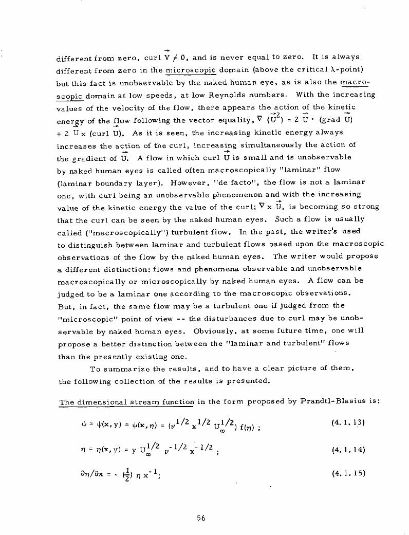
different from zero, curl V / 0, and is never equal to zero. It is always
different from zero in the microscopic domain (above the critical X-point)
but this fact is unobservable by the naked human eye, as is also the macro-
scopic domain at low speeds, at low Reynolds numbers. With the increasing
values of the velocity of the flow, there appears the action of the kinetic
enery of the flow following the vector equality, V (U ) = Z U - (grad U)
+ 2 Ux (curl U). As it is seen, the increasing kinetic energy always
increases the action of the curl, increasing simultaneously the action of
the gradient of U. A flow in which curl U is small and is unobservable
by naked human eyes is called often macroscopically "laminar" flow
(laminar boundary layer). However, "de facto", the flow is not a laminar
one, with curl being an unobservable phenomenon and with the increasing
value of the kinetic energy the value of the curl; V x U, is becoming so strong
that the curl can be seen by the naked human eyes. Such a flow is usually
called ("macroscopically") turbulent flow. In the past, the writer's used
to distinguish between laminar and turbulent flows based upon the macroscopic
observations of the flow by the naked human eyes. The writer would propose
a different distinction: flows and phenomena observable and unobservable
macroscopically or microscopically by naked human eyes. A flow can be
judged to be a laminar one according to the macroscopic observations.
But, in fact, the same flow may be a turbulent one if judged from the
"microscopic" point of view -- the disturbances due to curl may be unob-
servable by naked human eyes. Obviously, at some future time, one will
propose a better distinction between the "laminar and turbulent" flows
than the presently existing one.
To summarize the results, and to have a clear picture of them,
the following collection of the results is presented.
The dimensional stream function in the form proposed by Prandtl-Blasius is:
= (x, y) = (x, 7) = ( 1 / 2 x1/ U /2) f() . 13)
I = (x y U 2 -i/2 x- 1/2; (4.1.14)
a/ax = - ( - 1. (4. 1.15)
56
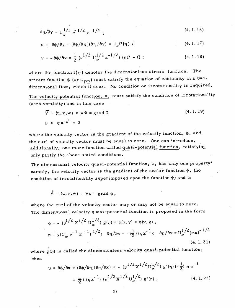
/ay 1/2 I1/ 1/2 (4. 1. 16)
u = 8a/8y = (84/8 )(r n / 8 y) - Uf' () ; (4. 1. 17)
v=-8 /8x = (v1/2 U 1/ 2 X 1/ f' -f) (4.1.18)
where the function f( rl) denotes the dimensionless stream function. The
stream function i (or PPB ) must satisfy the equation of continuity in a two-
dimensional flow, which it does. No condition on irrotationality is required.
The velocity potential function, D, must satisfy the condition of irrotationality
(zero vorticity) and in this case
V= (u,v,w) = V = grad (4. 1. 19)
w = VXV = 0
where the velocity vector is the gradient of the velocity function, #, and
the curl of velocity vector must be equal to zero. One can introduce,
additionally, one more function called quasi-potential function, satisfying
only partly the above stated conditions.
The dimensional velocity quasi-potential function, , has only one property'
namely, the velocity vector is the gradient of the scalar function , (no
condition of irrotationality superimposed upon the function f) and is
V = (u,v,w) = V4 = grad 5,
where the curl of the velocity vector may or may not be equal to zero.
The dimensional velocity quasi-potential function is proposed in the form
S= - (vI /2 X 1 / 2 U 1 / 2 ) g(1j) = (x,y) = (x, r) ,
(U -1 /2; a/x = - ()(x-); ,/ay = Ul/2 (x)-1/2n= y(Uv x -) 1 1 - (vx)
(4. 1.21)
where g(rl) is called the dimensionless velocity quasi-potential function;
then
1/2 1/2 1/2 1 -(aux /ar)(an/ax) = - (l X U' / ')' x
= () (x- 1 1(/2x1/2 U1/2) g'() ; (4. 1. 22)
57

-1 1/2
SUm (X x1 )1/2 g'() (4. 1.23)
2 -1 -1One can verify that, with v =cm sec , X = cm, UC0 cm sec , the
proper dimensions are preserved in the above equations for u and v,
Equations (4. 1. 22) and (4. 1. 23). For the velocity component u, Equation
(4. 1. 22) becomes
(x) / X UI =(cm sec )(cm )(cm sec )(cm
2 -1 -1) -1= (cm sec (cm
-1
which is correct. The velocity v also has dimensions = cm sec .
The definition of streamline can be found in von Mises, Glauert,
Owczarek and others. At each fixed time t, there is a (two-parameter)
family of streamlines; i. e., space curves described by moving particles.
For t = to each streamline is tangent at each point to the velocity vector
at this point or: dx: dy: dz = qx y: qz ' where qx denotes the velocity
component in x-direction and qx = qx(x,y,z,to), etc. Clearly the stream-
line through any point r at t = to , is tangent to the trajectory of the particle
through r at that instant [von Mises, pp. 4-5]. As the stream function
q satisfies the continuity equation, the curves of 4 = constant represent
streamlines. The relation
di = (84/8x) dx + (ap/a8y) dy = - v dx + u dy = 0 for L = constant
(4. 1. 24)(Owczarek, pp. 62-63);
is valid in a two-dimensional (temporarily fixed) flow at any period of
time due to the fact that
u = ai/ay; v = - a/ax. (4. 1. 25)
Equations derived above may allow one to pass from the notion of the
streamfunction, p(x,y), (dimensional), or f(7), (dimensionless), to
the concept of velocity potential functions, Z , or velocity functions
i(x,y), (dimensional), or g(), (dimensionless), and vice versa. From
Equations (4. 1. 22) and (4. 1. 5) one obtains
58

u () (rx) (x 1/2 /X U/) g' () = U f () . (4. 1.26)
From Equations (4. 1. 23) and the Prandtl-Blasius approach one obtains
v : U (X x- 1 1)/ g' () = U 2 1/2 x- 1/2 [r f '(r) - f(r)] . (4. 1.27)
Verification of the dimensions of various terms and factors in the present
work is repeated occasionally but done for precautionary purposes
so as to avoid possible mistakes.
In the above, the g'(r) denots a differentiation with respect to r.
One may verify the dimensions of the variables appearing in the problem,
if and when the dimensional variables are used:
-1 -1 -1u cm sec ; v = cm sec , U= cm sec
f = f(r) = dimensionless streanmfunction;
S= ~dimensionless coordinate; (x,y) = dimensional coordinate = cm;2 -1
= stream function = cm sec , since u = 8 P/y;2 -1
= velocity potential function = cm sec , since:
u= 80/x.
The variables and the coefficients appearing in the functions in question
are
= Uc/2 v 1/2 x- ; (dimensionless);2 -1
V = coefficient of kinematic viscosity = cm sec ;
= cm (cm/2 sec -1/2 )(cm-1 sec 1/2) cm- 1/2 = dimensionless;
/2 /2 /2- 1/2 1/2 1/2 - 1/2S= y x1/ U / f(r) = (cm sec ) cm cm sec
2 -1cm sec
The proposed form of the velocity qusi-potential function, Equation (4. 1. 6)
is
= - ( / 2 /2 x1/2 U 1 /2) g(n) , (4. 1.28)
where
X = constant length = cm;
59

and where g(j) may be called the dimensionless velocity quasi-potential
function. Thus
1/ x1/2 1/2 = (cm sec - /2 1/2 1/2 sec- 1/2)v X U = (cm sec ) cm (cm sec
= cm2 sec- 1 (4. 1. 29)
Verification of the coefficients of the velocity components, u and v
(Schlichting, p. 117) furnishes:-1
coefficient of u: u = Uf'(r); U. = cm sec ; (4. 1.30)
coefficient of v: v = (1/2 U1/2 x- 1/2 f - f) ; (4. 1. 31)
then
1/2 u1/2 1/2 = (cm sec- 1/2)(cml/2 sec- 1/2)(cr n - /2) cm sec-
(4. 1. 32)
V = grad = 7 (u,v) = velocity vector. From the definition of the
velocity quasi-potential function,
84/ax = (8/8ar)(8~/8x) = u ; (4. 1. 33)
8W/ay = (a84/8)(a/8y) v; (4. 1. 34)
where the derivatives, appearing in Equations (4. 1. 33) and (4. 1. 34), are:
a/arl = - (1/2 x1/2 U /2) d g(rj)/8n ; (4. 1. 35)
S= yU/Z -1/2 1/2 1/2; (8r/8x) -) x 1 (4. 1. 36)
S1/2 - 1/2 x 1/2 (4. 1.37)
thereby verifying the correctioness of the dimensions:
8= ,/r)(ari/Ox) = - (v X1/ U1/2)(d g (r)/d)(- x
1 (1/2 x1/2 U1/2) (I x 1) (d g(rl)/dr)
(cm sec- 1/2)(cml/ )(cm l / 2 sec- 1/2)(cm-l) cm sec-
(4. 1. 38)
60

since r is a dimensionless coordinate; and
v = (84/n)(an/ay)
- (v I / 2 X 1 / 2 UI / 2) (d g(rj)/dr))(8ri/8y)
(v l/2 X 1/2 U1/2) (d g())/dr)(Ul/2 1/2 x-1/2
-1/2 1/2 -1/2 1/2 -1/2(cm sec )(cm sec )(g'(r))(cm / sec-
(cm-1 se+1/ )(cm-1/2) = U (d g(r)/drj) = cm sec- 1
(4. 1. 39)
The relationship between the velocity quasi-potential function and stream
function f (f calculated numerically by Blasius) is proposed in the form
1 (vX Um)1/2 ( i 1) g(n) = Um '() (4. 1.40)
with the functions f = f(r)), f'(r) = df/dr), being calculated and tabulated
numerically in Schlichting's book (p. 121).
The approach to the calculation of the dimensionless velocity quasi-
potential function is done for illustrative purposes only. The reason for
the example is to demonstrate that anyone attempting to solve a problem
of this character may be unaware at the outset that there are great
differences in the absolute values of the velocity components u and v.
These functions must be used to calculate the value of the potential function.
The first step of the approach toward achieving this goal is demonstrated
below and consists of a process of multiplication quantitatively large functions
of u by quantitatively small functions of v. If these quantitative values are
not known initially, one may proceed in the manner given below by trying
to seek an average value.
From Equation (4. 1. 40) one gets:
g'(r) = 2 (V1/2 I/ X 1/2))(x - f( , (4. 1.41)
or
dg() = 2 (v- 1/2 X 1/2 U/2 r f'() dr. (4. 1.42)
Verifying the coefficient
S1/2 X- 1/2 U1/2 2 - 1 1/2 - 1/2 1/2 - 1/2(- X / U x/2 = (cm sec ) (cm )(cm sec ) cm
= dimensionless.
61

This is correct; because the function f'(rl) is not given in a closed form
(only in tabulated form) and thus the function g(rj) can only be calculated
by a numerical integration. An analogous approach is followed with
respect to the component v:
v = a/ay = - (v1/2 X 1 /2 U 1 /2) (d g(rj)/drj)(8ar/8y)
(v1/2 x1/2 u1/2)(g(r))(U1 2 V- 1/2 - 1/2
= - U (X x- 1 /2 g'(r)) * (4. 1.43)
On the other hand the variable v is given in the following form from the
Prandtl-Blasius theory (Schlichting, p. 117):
v =a - LB/x = (v /2 U/2 x- /2)( f-) . (4. 1. 44)
A comparison of the equations gives ((4. 1. 43) = (4.1. 44) ):
- U (X - 1/2 1/2 , 1 / 2 U -( 1/2 U/2 x 1/2)( f'-f) , (4. 1. 45)
where g'(r)), r~, f'(t), f, are dimensionless, and the coefficients on both
sides of the equation have dimensions since dimensional quantities for
the coordinates (x,X) and for the coefficient of kinematic viscosity are
used.
Thus-1 2 - 1/2 -1 1/2 -1/2
cm sec = (cm sec ) (cm sec ) (cm-
(cm sec 1/2) (cm/2 sec 1/2)(cm- 1/2= cm sec-1
(4. 1. 46)
which is correct; Equation (4. 1.45) gives:
- U (X x- 1)1/2 g'(77) 1= V/ U1/2 x 1/2) ( f'f) (4. 1.47)
or
g,(1) = - (V1/2 U-1/2 X-1/2) ( f4. 1.48)
where the coefficient on the right hand side has no dimensions . In reality,
in the case dimensional quantities are used the value becomes
2 -11/2 - -1/2 -1/2(cm 2 sec 11/2 (cm sec- 1/2 (cm- ) dimensionless. (4. 1. 49)
62

This is correct due to the fact that )~, f'(rj), f(yr), g'(r), are dimensionless
functions.
From Equation (4. 1. 48) one obtains:
1 1/2 -1/Z -1/2g'(+) = ( / ) U X- 1/2) (f - r f'). (4. 1. 50)
This obviously must be equal to Equation (4. 1. 41). When both sides of
Equations (4. 1. 41) and (4. 1. 50) are multiplied (i. e. , left by left, right
by right), respectively, one gets:
[g'(n)] = X (x rn ) f' (f - ) (4.1.51)
Or:
g- 11/2 1/2 [f() 1/2 (4. 1.52)
to find the function g(r]), Equation (4. 1. 52) must be integrated numerically.
In Equation (4. 1. 52) the quantities (x,X) must be measured in the same
units of length (cm) if one uses dimensional quantities.
The velocity quasi-potential function, 4( 1 ) , contains in its
structure, the dimensionless quasi-potential function g(rl ). The function
g(q) has to be calculated numerically by means of the dimensionless
stream function f(ir) and its derivatives f' and f" (if necessary). The
function f is a function of one independent, dimensionless coordinate, r7.2 2
Its derivatives involve only ordinary derivatives f', f" = d 2f/dr . The
relationship between the dimensionless velocity potential function g(r)
and the dimensionless stream function f and its derivative f' is given
in Equation (4. 1. 52). The involved integration has to be done numerically.
The following integration procedure is used:
The functions rl = r(x,y); f = f(rj); f' = f'(r7); f" = f"(rT), are
tabulated in the Schlichting book, p. 121.
First Step
These functions can be plotted graphically as functions of r.
The numerical tables of Schlichting are ordered according to the step-
wise variations of rl, which is the independent variable (coordinate).
Second Step
The second step of the numerical integration is to calculate the
63
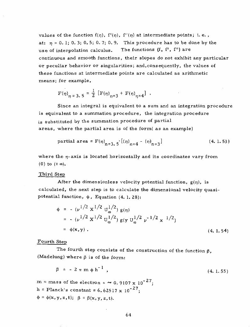
values of the function f(rj), f'(j), f"(~) at intermediate points; i. e.,
at: n = 0. 1; 0. 3; 0. 5; 0. 7; 0. 9. This procedure has to be done by the
use of interpolation calculus. The functions (f, f', f") are
continuous and smooth functions, their slopes do not exhibit any particular
or peculiar behavior or singularities; and,consequently, the values of
these functions at intermediate points are calculated as arithmetic
means; for example,
F(n)=3.5 = - [F(r) 3 + F(a)=4 ]
Since an integral is equivalent to a sum and an integration procedure
is equivalent to a summation procedure, the integration procedure
is substituted by the summation procedure of partial
areas, where the partial area is of the form( as an example)
partial area = F(-r)n=3. 5 [(l)n=4 (T)n=3] (4. 1. 53)
where the a-axis is located horizontally and its coordinates vary from
(0) to (+ c).
Third Step
After the dimensionless velocity potential function, g(r7), is
calculated, the next step is to calculate the dimensional velocity quasi-
potential function, 4, Equation (4. 1. 28):
S= - (vl/ X1/2 U/2) g(rn)
(z (1/2 X1/2 U1/z) g(y U/2 V-1/2 x 1/2)
= (x,y) . (4. 1.54)
Fourth Step
The fourth step consists of the construction of the function P,(Madelung) where P is of the form:
2- 1p = - 2 ,m h- (4. 1.55)
m = mass of the electron = N 0. 9107 x 10 - 2 7
h = Planck's constant = 6. 62517 x 10-27
= (x, y, z,t); = (x,y, z,t).
64
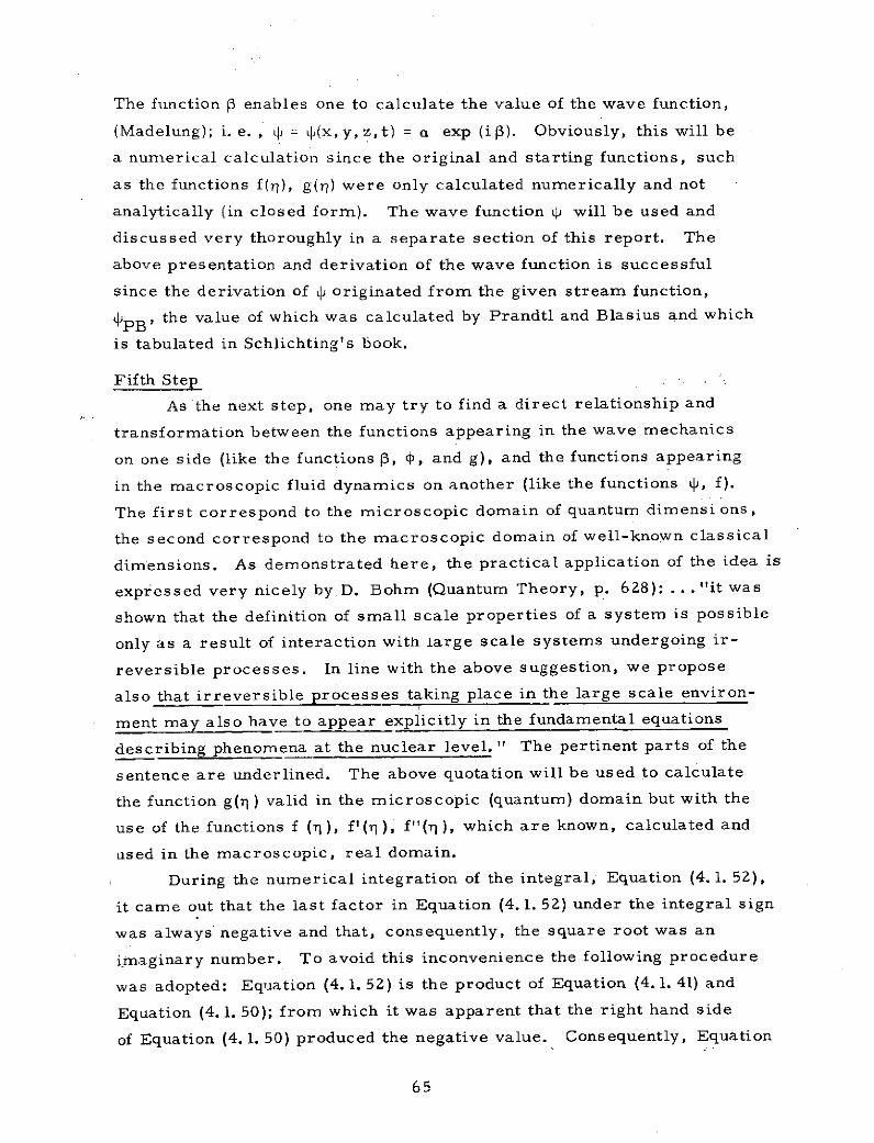
The function P enables one to calculate the value of the wave function,
(Madelung); i. e. , = (x,y,z,t) = a exp (i ). Obviously, this will be
a numerical calculation since the original and starting functions, such
as the functions f(a), g(7) were only calculated numerically and not
analytically (in closed form). The wave function L will be used and
discussed very thoroughly in a separate section of this report. The
above presentation and derivation of the wave function is successful
since the derivation of i originated from the given stream function,
qPB' the value of which was calculated by Prandtl and Blasius and which
is tabulated in Schlichting's book.
Fifth Step
As the next step, one may try to find a direct relationship and
transformation between the functions appearing in the wave mechanics
on one side (like the functions P, P, and g), and the functions appearing
in the macroscopic fluid dynamics on another (like the functions t, f).
The first correspond to the microscopic domain of quantum dimensi ons,
the second correspond to the macroscopic domain of well-known classical
dimensions. As demonstrated here, the practical application of the idea is
expressed very nicely by.D. Bohm (Quantum Theory, p. 628): ... "it was
shown that the definition of small scale properties of a system is possible
only as a result of interaction with large scale systems undergoing ir-
reversible processes. In line with the above suggestion, we propose
also that irreversible processes taking place in the large scale environ-
ment may also have to appear explicitly in the fundamental equations
describing phenomena at the nuclear level. " The pertinent parts of the
sentence are underlined. The above quotation will be used to calculate
the function g( ) valid in the microscopic (quantum) domain but with the
use of the functions f (ri), f'(r ), f"(r ), which are known, calculated and
used in the macroscopic, real domain.
During the numerical integration of the integral, Equation (4.1. 52),
it came out that the last factor in Equation (4.1. 52) under the integral sign
was always negative and that, consequently, the square root was an
imaginary number. To avoid this inconvenience the following procedure
was adopted: Equation (4. 1. 52) is the product of Equation (4. 1. 41) and
Equation (4.1. 50); from which it was apparent that the right hand side
of Equation (4. 1. 50) produced the negative value. Consequently, Equation
65

(4. 1. 50) is multiplied by (- 1) and written in the following form
(-1) g,(r) = (vl/2 U/2 X 1/2) (f' - f) from Eq. (4. 1.56)(4. 1. 50).
Next, Equation (4. 1. 41) is multiplied by Equation (4. 1. 56 ); i. e. , left
hand side of Equation (4. 1. 41) is multiplied by the left hand side of
Equation (4. 1. 56) and right hand side of Equation (4. 1. 41) is multiplied
by the right hand side of Equation (4. 1. 56) giving as the result
(-1) [g,(n)]2 = (X- ) (x 1 ) f(f', f) . (4. 1. 57)
The next operation involves taking the square root:
-1)1/2f/2 (/ ff1/
(NF- 1) g'(rj) = (X 1/2) (x ) (f 1 /2 1-f) . (4. 1.58)
Equation (4. 1. 58) corresponds to Equation (4. 1. 52) and the integration
furnishes:
i g() = (X- 1/2) (x r- 1)1/2 (f1)/2 (f' f)1/2 d , i = F-1 .
(4. 1.59)
This equation corresponds to integrated Equation (4.1. 52) but no longer has
the negative values in the last factor which item causes some difficulty
when performing numerical integration on the computer.
The above calculation of the function g(i) is equivalent to taking
a geometric mean value from the two values of g(v7): one given by
Equation (4. 1. 41) and the other given by Equation (4. 1. 50), respectively.
An analogous or similar result could be obtained by taking the arithmetic
mean from the two values of g(r7), one given by Equation (4. 1. 41) and
another by Equation (4. 1. 50), respectively. After performing the
integration on the right-hand side of Equation (4. 1.59), one ignores the
fact that the left-hand side is an imaginary one and considers only the
real part of the result.
The foregoing example demonstrates an approximate manner
of the calculation of the velocity potential function. The numerical
integration can be achieved according to one of two schemes as follows:
suppose that one wants to integrate the area under the curve y = f(x);
then the area can be divided into a certain number of strips having the
y-coordinates yo, yl, y 2 , and so on. The area of one strip is
66

A = Y/2 (b-a) , 4. 1.60)
or
A2 = (Y0 + Yl) [b-a] ;
where (b,a) are the x- coordinates of the limits (end points) of the strip
and where y0 ,Y 1 , correspond to (a,b), respectively; Yl/2 corresponds
to the point (a+b)/2, respectively. The error of the A 2 approach is
usually greater one than that of the A1 approach.
4. 2. Velocity Potential Function: Complex Variable Function
The second way of calculating the velocity potential function
involves the elements of the theory of complex variables. This approach
is not always appreciated but can be very valuable.
A single complex coordinate of a point is defined by the equation
z = x + iy = r (cos + i sin) ; i = -; (4. 2. 1)
cos O + i sin O = exp (i ) ; (4. 2.2)
z = r exp (i 0); r = modulus of z; (4.2.3)
r = mod z = iz I ; 0 = argument of z . (4. 2. 4)
Any function f(z) of the complex variable z can be separated into its
real and imaginary parts, and can be expressed in the form (X + i Y),
where X and Y are real. Consider a function of the complex variable z
which has a single valued differential coefficient at every point and
let
f(z) = 5 + in; d f/dz = p + i q (4. 2. 5)
then
p + i q = d f/dz = af/ax = 38/x + i a/8x , (4. 2. 6)
and
df/dz = i-1 af/y = - i 8/8y + a1/ay . (4.2. 7)
Hence
ag/ax a= /y = P , (4. 2. 8)
and
ag/ay = - /x =- q , (4.2. 9)
V2 V2 = = . (4.2. 10)
67

Introducing the velocity potential function, D , and the stream function,
4, one can combine these two into a complex velocity potential function:
w = f(z) = @ + i 4; dw/dz = u - i v ; (4.2. 11)
-4 =5 ; = ; 8a/ax = 8/8y = 8a/ax = 8/ay ; (4.2. 12)
S; ; ag/oy = - an/ax = /ay= - a/ax ; (4. 2. 13)
as /ax = at/ay = u ; (4. 2. 14)
a /ay = - a/ax =- v . (4. 2. 15)
The above formalism presents the fundamentals of the association of the
velocity potential function with the stream function [Glauert, pp. 53- 55]
in a two-dimensional fluid motion. Concerning the higher dimensional
space (three or more) some special propositions have to be used. These
will not be discussed at this time. Equations (4. 2. 14) and (4. 2. 15) give
an association between the function i, stream function, discussed in
previous sections, and the sought-after function, velocity potential, .•
As stated previously, the function 4 is known, and has been calculated
and tabulated in Schlichting's book. The function D must be found by
a numerical integration. The manner of achieving this will follow.
In general, when the function 4 is assumed to be known, the
values of the velocity components, u,v, can be found and calculated by
the analytical process of differentiation. For the sake of clarity, the
process of the detailed differentiation of the function 4 will be reproduced
below. The task will therefore be to calculate and to find the correct
value, or as close as possible, of the function (D ; i. e. , the velocity
potential function. This task is associated with an inverse process;
e. g. , process of integration.
(A) The stream function 4 must satisfy the continuity equation.
The proof is very simple, as taken from Schlichting, pp. 117, one has
u = U,f'(r); v U 1 / 2 1/2 x 1/2 ( f'-f) ; (4. 2. 16)
8u/ax = (au/ar)(8ar/ax) = U f"() (-I Y U1/2 1/2 X3/2)
1 - 1 r/2 1/2 1/2 (4. 2. 17)
68

1 1/2 /2 1/2 f) U 1/2 -1/2 -1/av/ay = (av/ar)(ar/ay) = uo / x (ff, - f)U 0 - x
1 U x- l1 f (4. 2. 18)
The sum of the two equations (4. 2. 17) and (4. 2. 18) is zero which is
correct.
(B) The velocity potential function stipulates that the flow is
is irrotational and the vorticity vanishes; i.e., w = Vx V = 0. In
simply connected regions the flow velocity vector in such flow is the
gradient of a single-valued scalar point function, 5 , called the velocity
potential function.
Thus the scalar point function, 0 , should be constructed in such a manner
as to furnish an irrotational or potential flow and its gradient should be
equal to the flow velocity vector. The velocity quasi-potential function
4' and the dimensionless velocity quasi-potential function, g(r)) have
been introduced to fulfill only one condition mentioned above; namely,
that the gradient should be equal to the flow velocity vector.
Returning to the problem of the complex velocity potential function,
Equations (4. 2. 5) to (4. 2. 15), respectively, one may repeat:
w = Q + i ; dw/dz = u - i v; u = a/8y ; (4.2. 19)
and
v =- a/ax; r = y U/ v- x- ; (4. 2. 20)
or:
(84)/8y = (a8/a)(a) /ay) ; (4. 2. 21)
a8/8x = (8/r/8)(r1/x) . (4. 2.22)
From the set of relations, derived above, one gets
8a/ax = 8al/ay = u; 8/8y = - 8/x = - v , (4. 2. 23)
which is in agreement with the statement that the real part must be equal
to the real part and the imaginary part must be equal to the imaginary part as
df/dz = af/ax = ac4/ax + i ap/ax
= i-1 af/ay = - i a /ay + a/ay ; (4. 2.24)
or
a)/ax = 8 /ay ; a8/8x = - a8/8y . (4. 2.25)
69

Another form of the above stated in equational form may be
a/ax + i ad/ay = 8h/ay - i 84q/ax (4. 2. 26)
or
a(P/ax=u ; a/ay=v ; (4. 2. 27)
a /ax=- v ; a4/ay = u . (4. 2. 28)
Thus
u + iv = u + iv (4. 2.29)
is obviously true. For purely formalistic purposes one can write:
de = (8a/8x) dx + (a8/y) dy
= udx+ vdy
= (ap/ay) dx - (84/ax) dy
= (akP/8 a)(arj/ay) dx - (8 1 /8r)(ar/x) dy
= U f'(ri) dx + 1 (U1/2 1/2 x- 1/2) (r7 f'-f) dy . (4. 2. 30)
Or:
Sd = U S f '( ) dx ++ (U /2 1/2 x-1/2)(frf'-f) dy (4. 2.31)
where one can establish the limits of integration from a to b, provided
that the upper and lower limits refer simultaneously to the composite
coordinate r = r(x,y), and the chosen Cartesian coordinates (x,y).
Thus:
= U f'() dx + ~ (/2 /2 x- 1/2)(Ylf'-f) dy .
a a a (4. 2.32 )
Neglecting the finite integrals and returning to the indefinite integrals
in Equation (4. 2. 32), and differentiating, one obtains
d = U f'(r) dx + - (U1/2 p1/2 x- 1/2)( f'-f) dy , (4.2.33)So 2 cm
which may be written in the form
de = (a~/8x) dx + (35/8y) dy . (4. 2.34 )
70

According to the definition of the velocity potential; i. e. , VQ = V, one
obtains
ax/ax = u; a/ay = v . (4. 2.35)
A comparison of Equations (4. 2. 33), (4. 2. 34), and (4. 2. 35), with the
results obtained previously in Equations (4. 2. 1) to (4. 2. 15)proves that
the approach is correct.
One may verify the last point of the previous analysis, namely,
irrotationality. According to the definition of the velocity potential
function, #, the scalar function b should furnish an irrotational flow;
. e. ,
V = V1; w =VxV = 0. (4. 2.36)
However, by means of numerical calculations it has been demonstrated
very thoroughly that curl V 0 ; i. e. , the curl V is never equal to zero
in the domain of the boundary layer under consideration (along flat plate).
Thus, the flow under discussion is quasi-potential. [V = V; Vx V t 0]
and the proper nomenclature for the function # was introduced earlier,
i. e., it was called "the velocity quasi-potential function.
(Equation (4. 2. 32) has to be solved numerically and the numerical
integration has to be achieved according to the scheme presented in
Section 4. 1. For a given value of y = 200 meters, 400 meters, etc.,values of and x(x/2 -1/2
one obtains values of and x(x x , etc.), and consequently the
values of x, y, and r] = t1 (x,y) are known. The knowledge of these
independent variables, (x,y) and of the composite independent variable
S=, r1 (x,y), allows one to use the formula (4. 1.54) to obtain the
approximate values of a function P = 4(). Thus, in the final step, one
calculates the sum of the two integrals, Equation (4. 2. 32). In place
of the numerical double integration process, it is proposed in the first
approximation that the sum of the two partial integrals, Equation (4. 2. 32)
be used: one numerically calculated in the x-direction and the other
numerically calculated in the y-direction.
4. 3. Diabatic Flow
In practice, the first assumption which has to be made is the
assumption referring to the kind of the fluid and the kind of the flow
which takes place in the phenomenon under consideration. The phenomenon
71

under the present consideration refers to the existence of the "laminar
boundary layer in a flow of a viscous ( consequently heat conducting
following the fundamental results of the kinetic theory of gases and
liquids) fluid medium. Due to the fact that the entire above approach is
applied to the domain of the flow of the fluid with the irreversible
phenomena (change of the kinetic energy into heat), the actual
physical picture is completely different from the mathematical abstraction
where there exists the concept of an ideal, reversible fluid flow with the
concept of the stream function. Some assumption and hypothesis must be
proposed in order to bring the above picture from the mathematical,
idealistic and even purely abstractive level back to the level of the real
fluid flow (irreversible phenomena, heat and energy dissipation). This
is done by a straightforward assumption which relates the flow to the
so-called "diabatic flow regime," where the irreversible phenomena-heat
and energy dissipation-can take place. The fundamentals and the theory
of "diabatic flow" were developed by NASA beginning in about 1944, and
since then many papers and reports have been published. The reader is
referred to the literature.
The term (m-lV?) in the equation proposed by Madelung represents,
according to the writer's assumption, the viscous irreversible forces
and dissipative phenomena. A more generalized form of the equation of
motion must include the action of the extraneous forces and action of the
dissipative forces as well. Put in such a form, the equation proposed by
Madelung may be considered to be representative of a class of generalized
equations of motion describing the motion of viscous, dissipative fluids
as described by the Navier-Stokes equation. The above simple and easy
explanation may also serve as an elementary explanation of the term of
"hidden variables" introduced by the late John von Neumann. Under this
term one should understand the physical action and the results of the physical
"forces," which are necessarily not only of a "constructive" or of a
"positive" or of an "accelerating" nature but may be also be of a "destructive"
or "negative" or "decelerative" nature (dissipative). The late John von
Neumann, in his book "Mathematische Grundlagen der Quanten-Mechanik, "
cites the Navier-Stokes equation and the Boltzmann-Maxwell equation as
being representatives of the equations of motion being expressed in terms
of "hidden variables. " The "hidden variables" express exactly the forces
72

which may be destructive, or negative, or decelerative or dissipative in-1
nature. In the present case the term m-1 V will represent the action and
the effects of all the terms containing the coefficient of viscosity.
Let one compare the equation proposed by Madelung with the
classical Euler's momentum equation in steady flow:
U. V + p VP - f = 0; f = extraneous force per unit
mass of the fluid; (4. 3. 1)
where P = static pressure.
For the sake of comparison, the reduced form of the Navier-Stokes
equation is used in describing the flow along an infinitely long flat plate in
which the fluid is assumed to be incompressible, and the conditions of the
flow are stationary:
u au/ax + v Du/ay = - p - 1 dp/dx + v (a 2u/ax2 + 2 u/ay2 ) (4. 3. 2)
In the flow in the boundary layer along a flat plate Prandtl-Blasius assumedthat the terms dp/dx and 82u/8x are so small that they can be neglected.Thus one gets:
u 8u/ax + v Ou/By - v 8au/y 2 = 0 . (4. 3.3)
Introducing the concept of the stream function in the classical sense,one obtains
S= (x, y, t); u = a84/y; v =- 8i/ax; (stream function). (4. 3. 4)
Then Equation (4. 3. 3) in the case of a steady flow with 8p/8x = 0 takesthe form [Schlichting, p. 114, Equation (7. 21)]:
at/ay a 2/axay - ap/ax a /ay 2- a 3/ay 3 = 0. (4. 3. 5)
To refresh the memory of the reader the wave equation and the sequence
of the equations are concurrently presented with the appropriate operations
obtained from the wave equation. The wave equation is:
V - 8 T2 m h- 2 ~- i 4 Tr mh- 1 8P/at = 0 ; (4.3. 6)
S= a exp (iP); a = a(x, y, z, t); p = P(x, y, z, t); (4. 3. 7)
73

0. 02517 x 101 cm-sec; (4. 3. 8)4 = - ph(2Trm)-1 _ (Z x n x 9. 107)
-27
h = (6. 62517 ± 0. 00023) x 1. 020 x 10 gr cm sec;
-27m = N 0. 9107 x 10 gr;
/8t + (V + + m- (VZ a) a h (8r2m 2 )1 = 0;
(4. 3. 9)U = v
2 + (a2 2 (4. 3. 10)v. (a V4) +a(a )/at = 0; a = p ;
V operator applied to (4. 3. 9):
1/at t+ (Z) + m-Vm - V[iVa- V2h2 (8 2m2)-] = 0; (4.3. 11)
V(i 2 ) = 2[FU Vt + x (Vx F)]. (4. 3. 12)
In the first approach Madelung assumed V x U = 0. The remaining
part of Equation (4. 3. 12) is inserted into Equation (4. 3. 9) thus giving
the equation corresponding to the equation of momentum in the reduced
form:
(U • V)U + m 1 = 0. (4. 3. 13)
The problem which now presents itself is to propose the scale magnification
factors which should enable one to associate the equations describing the
macroscopic phenomena with the equations describing the microscopic
phenomena (on the level of molecules and electrons). One may compare
two equations: one describing the phenomena on the macroscopic scale
as discussed in the boundary layer flow along a flat plate under stationary
conditions:
u 8u/8x + v 8u/ay + p dp/dx - v 8 u/yZ = 0 ; v = pp;(4. 3. 14)
the second one describing the same physical phenomena on the microscopic
scale:
(U • V) U + m- VQ = 0 . (4. 3. 15)
Since the symbol m denotes the mass of the electron, m = 0. 9107 x 1027
gram, one has to propose a scale magnification factor for "m, " as
discussed above.
74

5. SPECIAL MATHEMATICAL CONSIDERATIONS
5. 1. Some Characteristic Properties of Linear Systems
The advantages of the application of wave mechanics theory to
problems in fluid dynamics are the following: (1) the wave, Schroedinger,
equation is a linear partial differential equation, wherease the classical
Navier-Stokes equation is a highly nonlinear partial differential equation;
(2) the wave, Schroedinger, equation, initially and fundamentally, refers
to an electron which can be easily generalized, by means of an assumption,
to a cluster or an ensemble of particles grouped together around an
electron and guided by it; the concept of density appears usually
in the classical, macroscopic approach to the fluids. The cluster of
particles may be smaller in size than the number of particles in a
cubic centimeter, the factors defining density in any fluid or gaseous
medium. It is our impression that the natural phenomena in fluids and
gases do not always behave according to the rules established by classical,
deterministic fluid dynamics which are built around the concept of the
mass density. Occasionally, for some physical phenomena, the behavior
of liquids and gases may follow the rules of microscopic (wave, quantum
mechanics) fluid dynamics which are built on the concept of the cluster
of particles, i. e. , mass smaller than that referring to a cubic centimeter.
These phenomena may be investigated either by approaching a solution
from the macroscopic domain, mass per cubic centimeter (density) or
from the microscopic domain (the element mass such as the electron or
a cluster of particles grouped around the electron). Either approach is
appropriate; however, the present approach employes the method common
to the electron or the cluster of particles when grouped around a specific
electron, and then applying the concept to the density of the liquid.
This allows the use of wave mechanics from the very beginning. The
material in this section is intended to provide the background necessary
for the person who may not be fully acquainted with the characteristic
properties of linear partial differential systems or as a refresher for
the person who is fully acquainted with these properties. Obviously, no
such properties can be discussed for the nonlinear partial differential
system, since, in general, the present state of mathematics finds it
difficult to define correctly nonlinearity and nonlinear systems.
75

In particular the fundamental aspects of linearity and the law of
superposition are discussed. Differential equations are divided into
various categories and classes: ordinary differential equation refers
to an equation containing one or more ordinary derivatives; partial
differential equation refers to an equation in which the derivatives are
partial derivatives. From S. A. Havanessian, Louis A. Pipes, Digital
Computer Methods in Engineering, pp. 380-381, the ordinary differential
equation is, for example,
d2x/dtZ + Adx/dt + B x = O0, x = x(t);
whereas the partial differential equation is:
a2V/ax2 + a2V/8y + 8 V/az = 0, V = V(x, y, z)
Linearity and Superposition
Assume that a function u = u(x,t) is a sufficient differentiable
function of the arguments x and t. An operator represents an assignment
or transformation of one function to another by means of a set of
manipulations like differentiation, multiplication, addition, and
subtraction. Very often, the basic process is partial differentiation
and the operator in question is called a partial differential operator.
For brevity, such an operator is denoted by L, and the function it assigns
to a particular u by L[u]. The above operator has a very special property.
For example, it is noted that if u(x,t) and v(x,t) are any twice-differentiable
functions, then the same is true of a linear combination of these functions:
a u(x, t) + p v(x,t) , a = constant, p = constant; (5. 1. 1)
where a and p are any constants. Thus, the operator L[ a u + p v] and some of
its properties are defined below. By the rules of partial differentiation one has:
L[a u + p v] = a L[u] + p L[v] . (5. 1.2)
An operator having these properties is called a linear operator. It is
well-known that all operators (differential, algebraic, and possibly
others) are not linear. As a matter of fact, most physical problems
involve nonlinear operators; various simplifying assumptions
have to be made in order to replace a nonlinear operator
by a linear one. This is typical, in the sense that it is possible to
approximate the solutions of many problems by replacing nonlinear
76

by linear operators. An equation which equates L[u], where L is a
linear partial differential operator, to a given function F
L[u] = F (5. 1. 3)
is called a "linear partial differential equation. " A linear partial
differential equation with F - 0 is called a "homogeneous equation. "
An example of a linear partial differential operator is
a 2 2L[u] - c _ u(x,t) , (5. 1.4)
8t 8x
where c2 is a constant (Weinberger, pp. 30-31).
It is known that the unknown function u(x,t) is, in general, not
determined by the differential equation alone. One must prescribe
initial and/or boundary conditions. The transformation associating a
u(x,t) with its initial values u(x, 0) is also a linear operator, which one
may denote, say, by Ll[u].
Then
L 1 [u] E u(x,O) . (5. 1. 5)
Similarly:.
L 2 [u] = a (x, 0) (5. 1.6)
is a linear operator, as are:
L 3 [u] - u(0,t); L 4 [u] - u(,t) . (5. 1.7)
Assume the need to solve the initial-boundary value problem of the form
2/t 2 2 a 2u- c 2 = F(x,t), for O<x< 1, t > 0 ; (5. 1. 8)
ax
u(x, 0) = f(x), for 0 x I ; (5. I. 9)
au-t (x, 0) = g(x) , for 0 < x < I , (5.1. 10)
u(O,t) =0 , (5. 1. 11)
u(,t) = 0, i = constant . (5, 1. 12)
One may easily recognize that the above equation is the one-dimensional
wave equation, also called the one-dimensional vibrating string equation.
77
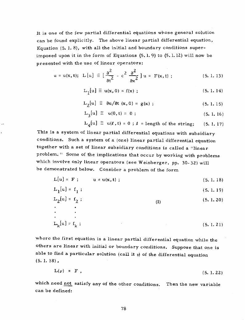
It is one of the few partial differential equations whose general solution
can be found explicitly. The above linear partial differential equation,
Equation (5. 1. 8), with all the initial and boundary conditions super-
imposed upon it in the form of Equations (5. 1. 9) to (5. 1. 12) will now be
presented with the use of linear operators:
2 2u = u(x, t); L[u] [ - c 2 - ] u = F(x,t) (5. 1. 13)
at 8x
L 1[u] u(x,0)= f(x) ; (5. 1. 14)
L 2 [u] 8au/at (x, 0) = g(x) ; (5. 1. 15)
L 3 [u] u(0, t)= 0 ; (5. 1. 16)
L 4[u] - u(,t) = 0 ; I = length of the string; (5. 1. 17)
This is a system of linear partial differential equations with subsidiaryconditions. Such a system of a (one) linear partial differential equationtogether with a set of linear subsidiary conditions is called a "linearproblem. " Some of the implications that occur by working with problemswhich involve only linear operators (see Weinberger, pp. 30-32) willbe demonstrated below. Consider a problem of the form
L[u] = F; u = u(x, t); (5. 1. 18)
L 1 [U] = f ; (5. 1. 19)
L 2 [U] = f (1) (5. 1. 20)
Lk[u]= fk (5. 1. 21)
where the first equation is a linear partial differential equation while theothers are linear with initial or boundary conditions. Suppose that one isable to find a particular solution (call it 1) of the differential equation(5. 1. 18),
L(v) = F , (5. 1. 22)
which need not satisfy any of the other conditions. Then the new variablecan be defined:
78

w = u-v. (5. 1.23)
From the linearity of the operator L one obtains the equation
L [w] = L[u] - L[v]= F - F = 0, (5. 1.24)
which states that the variable w satisfies a homogeneous differential
equation. Thus it has been shown that any solution u of the equation
L[u] = F can be written as the sum of any particular solution v of this
equation and a solution w of the corresponding homogeneous equation,
e. g. , from Equation (5. 1. 24):
u =w + v, (5. 1. 25)
L[u] = L[w] + L[v] . Q. E. D. (5. 1. 26)
Any solution of a homogeneous linear ordinary differential equation of
order "n" is a linear combination of n linearly independent solutions of
this equation. This is no longer true in the case of partial differential
equations. This fact accounts to a large extent for the vastly greater
difficulty in solving linear partial differential equations (Weinberg, p. 30).
The order and degree of a differential equation refer to the derivative of
highest order after the equation has been rationalized. Thus, the equation
d3y/dx 3 + x (dy/dx) /2 + x y = 0 (5. 1.27)
is of the third order and of the second degree, since when it is rationalized
it will contain the term (d3y/dx3). . If one now has a particular solution, v,
Equations (5. 1. 22), (5. 1. 23), and (5. 1. 24), i. e., L [v] = F, the problem
as discussed above, i. e. , Equations (5. 1. 18) to (5. 1. 21), can be reduced
to a new problem of the same kind, but with F = 0. By putting w = u - v,
one has from the linearity,
L(w) =0 ; (5. 1. 28)
L 1 (W) fl - L 1 (V) ; (5. 1. 29)
L 2 (w) = 2 - L () ; (II) (5. 1. 30)
L(w) = fk - L()
Lk(W) = fk - Lk() (5. 1. 31)
'9

In a similar manner, one may replace the system of Equations (5. 1. 18)
to (5. 1. 21) by a similar problem where some of the functions fl f' '" '
fk are zero by subtracting from u a function which satisfies some of
the boundary conditions.
The linearity of problem (I) can also be used to split it into a
number of simpler subproblems. Suppose that the function u 0 is the
solution of the system:
L[u o ] = F; (5. 1. 32)
L 1 [Uo ] = 0 ; (5. 1. 33)
L 2 [u o ] = 0 ; (5. 1. 34)
Lk[Uo ] = 0 ; (5. 1. 35)
and also that ul is the solution to an analogous system with some variations:
L[ul] = 0 ; (5. 1. 36)
L 1 [U1]= f 1 (5. 1. 37)
L 2 [Ul] = 0 ; (IV) (5. 1. 38)
Lk[U l] = 0 ; (5. 1. 39)
and that there are solutions for analogous conditions for u 2 , u 3 , ... , uk, then
each of the functions uo,Ul,... ,uk, involves only one piece of the data
F, flf 2" .' k' By linearity, one finds that the function,
u = u0 + u 1 + u 2 + ... + uk , (5. 1.40)
satisfies System (I), Equations (5. 1. 18) to (5. 1. 21). Thus, u is obtained
as a sum of terms each of which represents the effect of only one piece
of the data. In a particular case the final solution may represent a
decomposition into the effects of initial position, initial velocity, and
force (see Weinberger, p. 32).
Decomposition of Subproblems, Principle of Superposition
Each of the subproblems, discussed above, may in itself be1 2decomposed. Suppose there is a set of functions v , v ... , all of
which satisfy the same set of homogeneous equations, say:
80
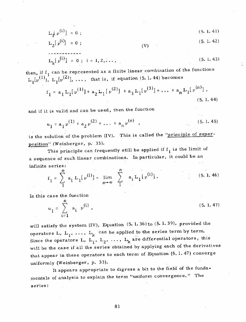
Ll[V(i)] = 0 ; (5. 1.41)
L 2 [ (i] 0 ; (V)(5.. 42)
Lk[(i)] 0 ; i 1,2,.. , (5.1.43)
then, if fl can be represented as a finite linear combination of the functions
L 11 (1)), Lv(2)], . . . , that is, if equation (5. 1. 44) becomes
fl alL (1)]+ a 2 1 (2)] + a 3 L 1[(3)]+ ... + anL 1 (n)
(5. 1. 44)
and if it is valid and can be used, then the function
u(1) + a (2) + + a V(n) (5. 1.45)
is the solution of the problem (IV). This is called the "principle of super-
position" (Weinberger, p. 33).
This principle can frequently still be applied if fl is the limit of
a sequence of such linear combinations. In particular, it could be an
infinite series:n
fl a Ll[) = lirm a i L [ i)] . (5. 1.46)Sn-, co
1 1
In this case the functionn
S(i) (5. 1. 47)u I = ai v ,
i=l
will satisfy the system (IV), Equation (5. 1. 3 6 ) to (5. 1. 39), provided the
operators L, L 1 , ... Lk can be applied to the series term by term.
Since the operators L, L 1 , L 2 , ... , Lk are differential operators, this
will be the case if all the series obtained by applying each of the derivatives
that appear in these operators to each term of Equation (5. 1. 47) converge
uniformly (Weinberger, p. 33).
It appears appropriate to digress a bit to the field of the funda-
mentals of analysis to explain the term "uniform convergence. " The
series:
81

a L [ v ( i ) (x) ] (5. 1. 48)
i=1
is said to converge uniformly on the interval a 5 x 5 b if for any E > 0
there exists an integer N(E) independent of x such that the following
inequality
m L [ v(i ) (x)] < E (5. 1. 49)
i=n+ 1
is preserved throughout the interval whenever n and m are larger than
N(E).
Uniqueness
A final simplification present in linear but not in nonlinear
problems occurs in the formulation of uniqueness and continuity theorems.
There is no intention to go deeply into the fundamentals of the analysis
of the basic fundamental theorems; consequently only a few remarks
on this subject will be given. Suppose that u and u are both solutions
of problem (I), Equations (5. 1. 18) to (5. 1. 21), then by linearity the
function v = (u - u) satisfies the homogeneous system:
L[ v] = 0 (5. 1. 50)
Ll ] = 0 (VI) (5. 1. 51)
Lk[ ] = 0 . (5. i1. 52)
System (VI) has the trivial solution v - 0. If this is its only
solution, then (u - u) must be identically zero; that is, the set (VI) has
at most one solution, but, of course, it could also have none. Suppose,
on the other hand, that there is a solution "v" of the set (VI) which is
not identically equal to zero, then if (VI) has a solution say, u, the
function (u + a v) , where a is any constant, is also a solution. That is,
the system (VI) cannot possibly have exactly one solution. It may have
no solution at all, or infinitely many solutions. Thus the uniqueness
problem for System (I), Equations (5. 1. 18) to (5. 1.21), is reduced
82

to that for the homogeneous (homogeneity of the problem set) problem the
latter System (VI), Equations (5. 1. 50) to (5. 1. 52). System
(VI) is independent of the particular data F, fl f2" " fk, which appear
in System (I), Equations (5. 1. 18) to (5. 1. 21) (see Weingerger,
pp. 30 to 34).
Continuity
The question of continuity of the linear systems of equations is
by no means trivial in nature but is of importance. Let u be a solution
of System (I), Equations (5. 1. 18) to (5. 1. 21), and let u be a solution
L[u] = ; (5. 1. 53)
L1[ ] = f ; (5. i1. 54)(VII)
L 2 [u] = T; (5. 1. 55)
Lkk[U] k;
The question: is it true that if
(F - F), (f f1 ) ' " (f - f ) (5. 1. 56)
are small, thedifference(u - u) is also small? If we let:
V = u- u; (5. 1. 57)
G =F- ; (5. 1. 58)
g = fl (VIII) (5. 1. 59)
g 2 = 1 - 1 ; (5. 1.60)
gi = g k ' (5. 1. 6 1)
then we see that the function v satisfies the problem (below):
L(v) =G ; (5. 1.62)
L (V) = g ; (X)(5. 1. 63)
L 2 (v) = g 2 ; (5. 1. 64)
Lk() = gk (5. 1.65)
The question, proposed above, now becomes: Is it true that the solution
83
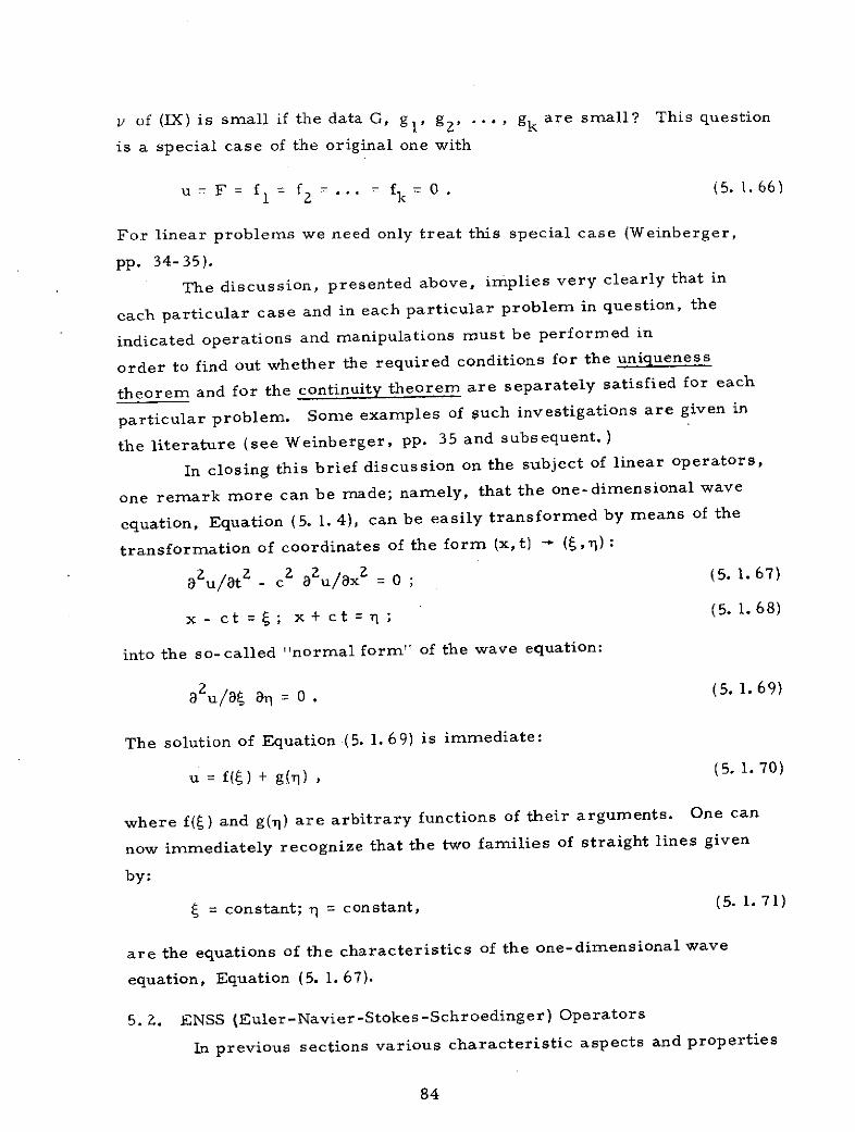
v of (IX) is small if the data G, gl' g2' ... , gk are small? This question
is a special case of the original one with
u = F = f " k = 0 . (5. 1. 66)
For linear problems we need only treat this special case (Weinberger,
pp. 34- 35).
The discussion, presented above, implies very clearly that in
each particular case and in each particular problem in question, the
indicated operations and manipulations must be performed in
order to find out whether the required conditions for the uniqueness
theorem and for the continuity theorem are separately satisfied for each
particular problem. Some examples of such investigations are given in
the literature (see Weinberger, pp. 35 and subsequent.)
In closing this brief discussion on the subject of linear operators,
one remark more can be made; namely, that the one-dimensional wave
equation, Equation (5. 1. 4), can be easily transformed by means of the
transformation of coordinates of the form (x,t) * (5, ?) :
8 u/atZ - c 8 u/ax = 0; (5. 1. 67)
x - ct = ; x + ct =1 ; (5. 1.68)
into the so-called "normal form" of the wave equation:
2 u/a a& = 0 . (5. 1.69)
The solution of Equation (5. 1. 69) is immediate:
u = f() + g() , (5. 1. 70)
where f() and g(,) are arbitrary functions of their arguments. One can
now immediately recognize that the two families of straight lines given
by:
S= constant; ti = constant, (5. 1. 71)
are the equations of the characteristics of the one-dimensional wave
equation, Equation (5. 1. 67).
5. 2. ENSS (Euler-Navier-Stokes-Schroedinger) Operators
In previous sections various characteristic aspects and properties
84

of linear differential equations (ordinary and partial) and of linear
operators were discussed. This section discusses the operations
involving special kind of operators, "wave mechanics operators" or
"Schroedinger operators," which are based primarily upon the fundamentals
of wave mechanics and the Schroedinger equation. The subject will be
presented very systematically, logically and orderly beginning with the
very fundamentals.
The medium under consideration, the fluid, is assumed to be a neutral
one obeying the Bose statistics. The fundamental equation upon which,
the entire formalism of the present wave mechanics approach is based is the
Schroedinger wave equation of the form
V2 - 8 i2 mh -2 J - i 4 rr mh - 8 B/8t = 0 , (5. 2. 1)
where the symbols used denote the following:
V 2 = Laplacian operator;
h = Planck's constant = 6. 54 x 10- 27 cm gram sec;
m = mass of the electron = 0. 9107 x 10 - 2 7 gram;
qJ = wave function; = 4( t, x, y, z) ;
S= potential energy of the field in which the entire above system
is located; D = D (t, x, y, z) is actually a function of the position
of the electron.
As suming, that
4 = a exp (iP); a = a (x, y, z, t); = (x,y,z,t) , (5. 2.2)
Madelung obtained two equations (real and imaginary parts, (R), (I)),
respectively:
+ 1 12 - 2 -1 2 2 2-118t (V ) 2 + m - (V 2 ) a- h 2 (8 2 )- = 0 ; (R) ; (5. 2. 3)
2 2V * (a2 V4) + a(a )/at = 0 ; (I) (5. 2.4)
= - Ph(2 m) = - CI 1 p; C 1 = h(2wm) - 1 ; (5.2.5)
where C l was a constant. With U = Vp and V x U = 0, Equation (5. 2.3)was modeled by Madelung to be equivalent to the Euler equation of motion,
2and Equation (5. 2. 4) with a = p (density of the fluid) as being equivalent
to the equation of the conservation of mass of the fluid
85

(continuity). In order to obtain the full form of the equations in question,
one has to apply one more formal operation; i. e. , a gradient operation
to Equation (5. 2. 3);
v(Vp) 2 = 2 [LT. VC+ U x (Vx U)]; (5. 2.6)
v(V~) 2 = 2 U t Vf if (Vx U) = ; (5. 2. 7)
V(V2 = 2 Ux (Vx F) if VU = 0. (5. 2. 8)
Of course, one could preserve both terms in Equation (5. 2. 6); e. g. ,
gradient and curl. In order to associate the field of Quantum Mechanics
with the field of Fluid Mechanics in the macroscopic sense, Madelung
accepted Equation (5. 2. 7) as the guide for his approach. In this way
he was able to associate the Schroedinger equation, Equation (5. 2. 1),
with the Euler equation of motion,
1 2 -1 -1 2 2 2 2-1aiU/at + - V( 2 ) + m- 1 V - V(a- V a h (8T m) - = 0 . (5. 2. 9)
Madelung proposed the following interpretation of various terms in
Equation (5. 2. 9): the term m- IVD represents the extraneous force
field, p- If , acting upon the medium in question; and the term
a- 1V2 a h2 (8 Tr2 m2 1 is associated with the action of the static
pressure; i. e. , S p- dp. In the conventional approach to the mechanics
and/or dynamics of viscous fluids in the macroscopic domain, one is
inclined to apply the Navier-Stokes system of equations to describe and
to deal with the phenomena in the macroscopic domain. Although
several other forms of equations such as the Burnett equations, attempt
to describe more or less accurately, the physical phenomena in viscous
liquids and gases. The Navier-Stokes system of equations still seems
to be considered as being the best one for these purposes. Some
mathematicians and physicists have devoted lifetimes to
selecting what they felt was possibly the best system of equations from
all the existing systems of equations from one or more fields of mechanics
and physics (mechanics of continuous media, mechanics of liquids, of
gases, kinetic theory of gases, molecular theory of gases and possibly
others Almost unaminously they agree that the Navier-Stokes system
of equations best fulfills the needs in the macroscopic; i. e. , observable,
domain for describing the physical phenomena of viscous fluids.
86

Professor George Uhlenbeck, well-known physicist, previously from the
University of Michigan, Ann Arbor, now Rockefeller Institute, New York,
expressed this opinion during theEighth International Symposium on
Rarefied Gas Dynamics, Stanford University, Stanford, California,
July 10-14, 1972.
Another item which is important to the reader is the fact that
the Schroedinger equation is a linear equation in the complex domain in
the fully mathematical, analytical sense of this word. After the choice
of the wave function was made by Irving Madelung (1926) in the form
of Equation (5. 2. 2) and following some formal operations of the purely
analytical nature such as taking the gradient, and after the decomposition
of the Schroedinger equation into the real part (R) and the imaginary
part (I), he obtained the Euler equation of motion which is a nonlinear
equation. Such behavior of the partial differential equation in passing
from one field of physics such as microscopic quantum mechanics to
another field such as macroscopic fluid mechanics is not new. In the
past it was signaled more than once that the passage (transfer) of the
Schroedinger equation from one field of physics to another field could
be associated with the change of the associated classification of the
partial differential equations concerning linearity or nonlinearity.
This fact must be kept in mind when changes, like the quantum mechanics
to mechanics or the reverse, are considered. This assumption (or
conjecture) is the basis for the proposed association and relationship
between quantum mechanics of viscous fluids based on the acceptance
of the validity of the systems obeying. the rules of diabatic flows.
The ideas of diabatic flow systems and of extending the Madelung
"quantum theory modification and application to macroscopic fluid dynamics,
including the domain of ideal fluid systems and viscous fluid systems, are
fundamentally and deeply rooted in ideas expressed by John von Neumann
in his immortal work, "Mathematical Foundations of Quantum Mechanics. "
In this work von Neumann proposed the idea of "hidden variables" as
one of the concepts of modern mechanics. As examples, he quoted the
Navier-Stokes system of equations and the Maxwell-Boltzmann (Burnett)
system of equations as being in some way representative of his concept
of "hidden variables" in the field of fluid dynamics.
Returning to the problem of the association of the quantum theory,
87

Schroedinger equation with the macroscopic fluid dynamics, Navier-Stokes
equation, one may demonstrate that the results obtained previously can
be obtained in another manner as well. Let one assume that the starting
point is through use of the Euler equation of motion (Owczarek, p. 65):
a8V/at+ V - 1VP- f 0 ; (5.2. 10)P
where the vector f denotes the vector force field acting upon the particle
in question. Making use of the vector relation (Owczarek, p. 52)
V. VV= wxV+V V); W=VxV , (5.2.11)
if J denotes the vorticity vector, one gets another form of the equation
where additionally one may include the action of the static pressure:
av/at + w xV + V( V) + VP - f =0 , (5.2. 12)2 P
where the symbol P denotes the static pressure in the fluid. When the
dissipative action and forces are taken into account and are superimposed
upon the field of an inviscid (non-heat conducting) fluid, the Euler equation
transforms into the Navier-Stokes equation (or an analogous one). One
of the acceptable forms of the Navier-Stokes equation is the following
one (Owczarek, p. 542):
12 2p [a/at+ xv + 2 V-v )]+VP-p +-f V(pY * V)
- 2 (V~) V V- (V ) x (Vx V) - [V 2V + V(V V)] = 0,
(5.2. 13)
where . is the coefficient of viscosity which usually depends upon the
temperature field and f , the gravitational force field.
The problem is to associate equation (5. 2. 13) with
the Schroedinger equation and its transformation as was performed by
Madelung, Equations (5. 2. 1) to (5. 2. 7). The guiding points are the
following:
(a) The finite system to be developed has to be a linear system
for the simple reason that the mathematical analysis , at the present
time at least, can only handle linear systems.
88

(b) The Madelung proposition will be used to associate,
i. e. , to construct a link or a bridge between linear wave mechanics,
the Schroedinger equation, and the nonlinear equation of motion of
an inviscid, non-heat conducting (ideal) fluid, the Euler equation.
(c) In general, theassociation presented above allows one to
generalize the above fundamental association,(Schroedinger- Euler) or
(Euler-Schroedinger),to other kinds of equations like Navier-Stokes.
Thus a bridge is proposed between the (Navier-Stokes-Schroedinger) or
(Schroedinger-Navier-Stokes), i.e.,the linear wave mechanics equation
and the nonlinear equation of viscous and heat conducting fluid
(real fluidL
(d) To achieve this goal from the fundamental point of view, an
assumption has to be made that the fluid system under consideration
follows the rules of the diabatic flow system, proposed by NASA
around 1944 and later. In this sytem the dissipative phenomena due
to the factor of viscosity and heat conductivity appear; the system,
so proposed, denoted as (Euler-Navier-Stokes-Schroedinger) is
treated in an analogous (but not identical) manner to the previously
mentioned (Euler-Schroedinger) system.
(e) The added system, the Navier-Stokes system, attached to
the chain (Euler-Schroedinger) system, when treated alone is a nonlinear
system of differential equations. The first terms of this system (see
Equation (5. 2. 13)) (disregarding the terms containing the viscosity
coefficient ), are identical with the terms existing in the Madelung
remodeling of the Schroedinger equation, and the Euler form of the
equation of motion (Equations (5. 2. 1) to (5. 2. 7)) (the Euler equation
is not linear). By his proposition, Madelung succeeded in obtaining a
chain (an association) between the Euler (nonlinear) and Schroedinger
(linear) equations, thereby obtaining some sort of "linearization" of the
nonlinear Euler equation of motion. This will now be called the
"Madelung linearization process" of the Euler equation of motion.
(f) The terms in the Navier-Stokes equation, containing the
viscosity coefficient 1, Equation (5. 2. 13) , are, in general, nonlinear
terms, since the coefficient pt is a function of the temperature field.
In thermodynamics the'pressure, temperature, and volume of a given
system are measured and are referred to as the thermodynamic
89

characteristic quantities of any given system. In very small regions
of space, especially near the "critical" point, change or passage from
the super-fluid state to the ordinary hydrodynamics status, it is
found that these thermodynamic quantities no longer obey exactly an
equation of state regardless of form in which it is considered. Instead
they exhibit large random fluctuations about a mean value that is predicted
by the equation of state. Hence, the deterministic laws of thermodynamics
break down and have to be replaced by laws of probability. This is so,
because the thermodynamic variables are no longer appropriate for the
particular problem and must be replaced by the position and velocity of
each molecule, which turn out to be, from the viewpoint of thermo-
dynamics, "hidden variables" (Bohm, p. 29). As stated before, the
term "hidden variables" was introduced by John von Neumann (see
references) and is used by Bohm and other quantum physicists. The
thermodynamic quantities are, then, merely averages of "hidden
variables" that cannot be observed by thermodynamic methods alone.
To find the underlying "causal" laws, one must accept a description in
terms of the individual molecules. Since this is usually a
practical impossibility one has to refer to actual, physical
experiments and to express the experimental ceofficients such as the
viscosity coefficient and the heat conductivity coefficient in terms of
thermodynamic quantities. These are, as stated above, merely averages of
"hidden variables" that cannot be observed by thermodynamic methods
alone. Thus, in the final conclusion, the coefficients of viscosity and
heat conductivity are necessarily experimentally measured and tabulated.
This is the reason why some quantum physicists and mathematicians
call the fundamental equations used in the macroscopic theory of fluid
dynamics, expressed in terms of the coefficients of viscosity and of
heat conductivity, "the equations in terms of hidden variables. " The
family of equations in this category may include:
(1) The Navier-Stokes system of equations of viscous, heat-
conducting fluid;
(2) The Burnett equations derived according to the molecular
theory of gases (see Patterson, reference);
(3) Another possible set of equations based upon the method of
Hilbert-Enskog-Chapman-Burnett (see Patterson, reference);
90

(4) Any other set of equations derived in a similar way which
uses both the above mentioned coefficients of viscosity and
heat conductivity in its derivation.
Returning to the Navier-Stokes system, Equation (5. 2. 13) and a
combined (Euler-Navier- Stokes-Schroedinger) system, one can start
from the simplest possible case, wherethe density of the fluid, p, and
its coefficient of viscosity, pL, are constant in magnitudes. In such
a case, consider the terms which appear on the left-hand side;
namely the two terms nonlinear in the function ', as from
Equation (5. 2. 11):
. . .0 1 2 -eV * VV x V + V ( V ) with = V x V . (5. 2. 14)
In this equation all the terms, expressed in terms of the unknown vector
function V are equivalent to the terms in the wave equation by using the
chain of substitutions, Equations (5. 2. 1), (5. 2. 6), and (5. 2. 9).
Basically, these substitutions do not change the physical nature and
the physical character of the equation. The changes introduced are
formalistic in nature, such as an operation on the square of the gradient,
( v ) , Equation (5. 2. 6), which have their origin in the particular kind
of operation on the Schroedinger equation and the form and interpretation
of the wave function, Equation (5. 2. 2) as chosen and proposed by Madelung.
By this kind of selection and proposition, Madelung could not and did
not change (or influence) the fact that the nonlinear terms mentioned
are always associated with and refer to the linear wave equation.
This process cannot be considered to be a general method of
linearization of the nonlinear differential equation, but in this special
case, the nonlinear Navier-Stokes equation, Equation (5. 2. 13), under
the assumed conditions (p = constant, . = constant), can be associated
with the combined (Euler-Navier- Stokes-Schroedinger) system of
equations and can be treated as one of the members of the family of the
(Euler- Navier- Stokes- Schroedinger) system. Consequently, Equation
(5. 2. 13) can be treated as a linear equation. It should be emphasized
again and again that Equation (5. 2. 13) is included in the family of the
linear equations because, and only because of the association of
Equation (5. 2. 13) with the Schroedinger linear wave equation by means
of the Madelung process of linearization. Assuming that the static
91

pressure P is calculable by use of the equation of state, P = Rp T, where
R = gas constant, p = constant (given), T = given, or that P is constant or, a
given function and that the vector functionl is given and known, then one can
safely assume that the Navier-Stokes equation, Equation (5. 2. 13),
belonging to the family of the (Euler-Navier-Stokes-Schroedinger)
system of equations, is a linear equation. This certainly is a major
achievement of the Madelung proposition, (Quantentheorie in Hydro-
dynamischer Form) published as long ago as 1926. A short-cut for
the chain of names (Euler-Navier-Stokes-Schroedinger) in the form of
the abbreviation (ENSS) will be used. The use of the symbolic notation
for the terms in Equation (5. 2. 14) is proposed; namely, the (ENSS)
differential operator, (ENSS)L :
(ENSS)LV =[w x+(V V)]V . (5. 2. 15)
Operating on the vector function V, one easily obtains from Equation
(5. 2. 13).for the coiastant values of p and p:
p {a/8t + (ENSS)L} V+ VP - p f = F ; (5. 2. 16)
or
p {3/8t + (ENSS) L} + VP - p f - F = O ; (5. 2. 17)
2 3 (V t) - [(V V) + V(V )]; (5. 2. 18)
where L= constant; p = constant. (5. 2. 19)
Moreover, due to the law of the conservation of mass (the equation of
continuity) for the media in which one assumes that p = constant,
V V= 0.
Once again it should be emphasized that all of the above operations
are purely formalistic operations and their sequence can be easily
reversed in order to start with the equation of motion of Euler and
return to the wave equation of Schroedinger. However, the wave equation
is a linear equation and consequently, the entire chain of operations
presented and discussed above must be considered as a chain of
formalistic operations on a linear system of mutually reversible related
operations. During these operations and due to the term (V ), the term
92

(V" grad V) appears which can be considered as the most important step
in the entire sequence of operations. Thus one can easily go from the
Euler equation of motion back to the wave equation by applying the chain
of formal operations in the reverse direction. This whole sequence and
system of operations is very logical and it proves one thing; namely,
that in its nature the entire system and set of operations existing in
the (ENSS) L operator is a linear system, because it has its origin in
the Schroedinger linear wave equation. One link in the entire system
having the form (V ' grad V), relates the Euler equation of motion to
the field of hydrodynamics. The history of modern quantum field theory
has demonstrated on more than one ocassion the very peculiar nature
and behavior of the wave fundamental mechanics equation of Schroedinger;
namely, that a chain of purely formal, very simple operations applied
to the wave mechanics equation of Schroedinger (linear) culminates in
the equation which, from the purely mathematical point of view, is
formally a nonlinear differential equation; but which, from the purely
physical point of view, expresses well the physical phenomenon at a
given moment and for a given set of circumstances (such as the boundary
conditions, the initial conditions, and so on).
Returning to the Navier-Stokes equation, Equation (5. 2. 13), or
Equation (5. 2. 16), or Equation (5. 2. 17), the (ENSS) L - operator is
instroduced in Equation (5. 2. 15);
p (a/at + (ENSS) L} V + VP - p f + F = 0 ; (5. 2. 20)
(ENSS) L = [w x+ (V V)] V ; (5.2.21)
2 2F = 3V(V . V) - [(V V-+ V(V. V)]; (5. 2. 22)
where p = constant; . = constant; P, f = known, given; V V = 0
It should be mentioned that, for the present at least, it is
difficult to include any differential equation, ordinary or partial,
directly without any discussion of the category of nonlinear or linear
equations. In December 1971 at the Annual Meeting of the American
Association for the Advancement of Sciences in Philadelphia, a special
session on the "Nonlinear Problem " was organized at which the investigator
93

was one of the invited speakers. During this session he presented a
discussion on "An Association Between the Wave Mechanics and the
Nonlinear Phenomena in Classical Mechanics by Means of the Quantum
Field Theoretic Methods in Statistical Physics. " Among the many
statements and conclusions, one result is particularly worthy of mention;
vis. , that up to the present time mathematics does not know exactly ,
how to define and how to classify the concept of nonlinearity. One thing
is certain, namely, that if a differential equation, ordinary or partial,
or an algebraic equation is definitely and absolutely not linear,
then it is certainly a nonlinear one. " From the point of view of the
concept of classifications, this appears to be a weak manner of
classification.
In this research the class of (ENSS) differential L operators is
included in the class of linear operators. One may consider also that
the properties of Equation (5. 2. 20), the equation to be investigated,
involve stationary conditions; i. e. , (i. e. , (a/at) is neglected. The
assumption of the stationary conditions implies that
VP = 0 (5. 2.23)
and that the fluid mechanics system in question is a
diabatic system, i. e. , that the terms (- pf + F) in Equation (5. 2. 20)
represent the dissipative forces. With pp- = v, and v * V = 0
(incompressible flow medium), Equation (5. 2. 17) takes the form
- 2 --0[(ENSS)L] V - vV V = 0 . (5. 2. 24)
This is considered to be a linear system and as such it corresponds
to Equation (5. 1. 3) above.
If L[u] = F, u = u(x,t), x = vector in n-dimensional space, (5. 2. 25)
and if Equation (5. 2. 24) is added to the "linear boundary problem"
as expressed in Equation (5. 1. 21), then one gets
L[u] = F; L1 [u] = fl; Lk[U] = fk (5. 2. 26)
Following the laws and rules of the linear problem, explained so thoroughly
above, one can continue the discussion of the linear problem, Equations
(5. 2. 25) and (5. 2. 26). Suppose one can find a particular solution "v"
94

of the differential equation
L(v) = F , (5. 1. 22) = (5. 2. 27)
which need not satisfy any of the other conditions. Then from Equation
(5. 1. 23) one gets:
w u - v; L [w]= 0, (5. 2. 28)
where w = satisfies homogeneous equation.
After one opens the (ENSS) L - operator in Equation (5. 2. 24) one gets
with the use of Equation (5. 2. 15):
[W x + (V - V)] V - v V2 = 0 , (5.2. 29)
and with:
V =i u+ j v+k w;
u = u(x,y); v = v(x,y); w = w(x,y); w = 0 ; (5. 2. 30)
= VxV ; (5.2. 31)
= Vx = T(aw/ay - v/az) + 3 (u/az - aw/ax) + k (v/x - u/ay) ;
(5. 2. 32)
W (W1' W 3 ) ; 1 = 0 ; 2 =0; 03 0 ; (5. 2. 33)
S j k
to xV= 1 2 3 (5. 2. 34)
u v w
WO x V = i (o2 w - o 3 v ) + j (Wo3u - w) + k(to 1 - 2u) ; (5. 2. 36)
consequently in the present case one has:
w x V =i (- w 3 ) 3 u) + 0 . 5. 2.37)
95
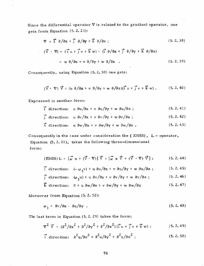
Since the differential operator V is related to the gradient operator, one
gets from Equation (5. 2. 21):
v =: a/ax + a/ay + k a/a8 ; (5. 2. 38)
S V)= (iu+jv+kw) (i 8/x +j a/y +k a/8z)
u 8/8x + v 8/8y + w a/az (5. 2. 39)
Consequently, using Equation (5. 2. 30) one gets:
(V - V) V = (u a/ax + v a/ay + w a/az)(i u + j v + k w) . (5. 2. 40)
Expressed in another form:
i direction: u au/ax + v au/ay + w au/az ; (5. 2. 41)
3 direction: u av/ax + v av/ay + w av/az ; (5. 2. 42)
k direction: u aw/ax + v aw/ay + w aw/az . (5. 2. 43)
Consequently in the case under consideration the ( ENSS) , L - operator,
Equation (5. 2. 21), takes the following three-dimensional
form:
(ENSS)L = [ x + (V. V)] V = [w x V + (V V) V ] : (5. 2.44)
i direction: (- w 3 v) + u au/ax + v au/ay + w au/az ; (5. 2.45)
j direction: (03u) + u av/ax + v av/ay + w av/az ; (5. 2.46)
k direction: 0 + u aw/ax + v aw/ay + w aw/az (5. 2. 47)
Moreover from Equation (5. 2. 32):
03 = av/ax - au/ay . (5. 2. 48)
The last term in Equation (5. 2. 29) takes the form:
2-= (a2/ax2 22 2 2 2 -:0-V V (2/x2 + a 2 /z2) (u + v + k w) : (5. 2.49)
i direction: a u/ax + au/ay + a 2u/az2 ; (5. 2. 50)
96

direction: a v/ax 2 + av/ay + av/az2 ; (5. 2. 51)
k direction: 3 w/x2 + a w/ay + a w/z . (5. 2. 52)
Thus, the full form of the vector equation, Equation (5. 2. 29), containing
the (ENSS) L - operator has the following three components:
i direction: (- w3 v) + u au/ax + v au/ay + w au/a z
- (8 2u/ax2 + a2u/ay 2 + 82 u/az 2) = 0 ; (5. 2. 53)
j direction: (w3 u) + u av/ax + v av/ay + w av/a z
- v (a2v/ax 2 + 2v/ay + 8 2 v/8z2) = 0 ; (5. 2. 54)
k direction: u 8w/8x + v aw/ay + w bw/8 z
- (2w/x 2 + a w/y 2 + a 2w/az2) = 0 . (5. 2. 55)
The above components of the (ENSS) L - operator refer to the Navier-Stokes
end of the chain of operations which obey the rules of the (ENSS) L - operator.
It may be of interest to present the beginning; i. e. , the first link in the chain
in question, in this case the Schroedinger equation. To demonstrate this,
we return to Equation (5. 2. 3), (5. 2. 6), and (5. 2. 9) in the stationary2
conditions, with the constant factor a = p (density) or to the system of
equivalent equations, Equations (5. 2. 10), (5. 2. 11), (5. 2. 12), and (5. 2. 20)
with VP = 0 and with (-pf + F) representing the dissipative forces, then
from Equation (5. 2. 20):
. -. 1 2 +
Sx V + V V ) - p f + F = 0. (5. 2. 56)
Thus we are back at the starting point; i. e. , the Schroedinger form of
equations, Equations (5. 2. 1), (5. 2. 3), where, in every case, one should
use the identity U - V. As is clearly seen, the nature of the mathematical
operations (see Equations (5. 2. 11) and (5. 2. 14))is such that in the entire
chain of operations and in the (ENSS) L - operator, the curl operation
and the gradient operation, see Equation (5. 2. 11), always appear
simultaneously:
I 2 - -V .VV = x V + V ); =Vx V; (5. 2. 57)
or (5.2.11) E (5. 2. 57)
or grad (V • V) = grad (V2) - 2(V . gradV + V x curl V). (5. 2. 58)
97

Thus, the appearance of the vorticity, circulation is a natural phenomenon
in viscous fluid motions due to the physical characteristic properties of
the coefficient of viscosity defined as the natural, transverse transport
of momentum. All of the natural, existing fluids in the macroscopic,
observable domain are viscous (inviscid fluids do not exist at normal
temperatures. Consequently, the vorticity, curl, phenomena in viscous
fluids often associated with the turbulence phenomena are "natural"
phenomena. The difference between the turbulence phenomena in micro
and macro circumstances is due to the varying degrees of observability,
(the possibility of observing the turbulence phenomena) since turbulence
phenomena cannot always be visually observed.
Equation (5. 2. 58) is an elementary, simple vector equation based
upon the fundamental principles of mathematical vector analysis. It
states that the two considered operations, grad and curl, always appear
together, thus confirming the results obtained from the point of view of
pure physics. Stated briefly, laminar flow does not and cannot exist in
viscous fluids in the macroscopic flow domain at the temperatures and
pressures above the phase transition, X-point. The kind of flow which can
exist under these circumstances can only be the turbulent flow of a varying
degree of turbulence, visually observable or unobservable. Neither Reynolds
in 1883, Prandtl in 1904, Blasius in 1908 nor G. I. Taylor in 1935
emphasized visually observable domain above the \-point. Madelung in
1926 mentioned the association of quantum theory with the Euler equation
of motion in inviscid fluid flow in the macroscopic domain. The explanation
of the attitude of all other writers (Reynolds, Prandtl, et al. ) is very
simple; namely, at the time those writers were working and writing on
the subject, neither they nor the science itself knew anything about
superfluidity, X-phase transition point, and so on.
Returning to the first equation derived above, i. e. , Equation (5. 2. 24):
[(ENSS) L] V - v V = 0, (ENSS) LV =[V x + (V. V)]; (5. 2. 59)
when in particular, the x-component of this vector equation is:
- w 3 v + u 8u/8x + v 8u/8y + w 8u/8z
- v(au/ax + 82u/y Z + 8 Zu/8z ) = 0; (5. 2. 60)
98

then for a two-dimensional flow in the boundary layer along an infinitely
long flat plate, Equation (5. 2. 60) is reduced to:
- 3 v + u au/ax + v au/ay - v(au/ax+ au/ay ) = 0 ;
3 = Ov/ax - au/ay . (5. 2. 61)
Equation (5. 2. 61) is not identical to the reduced equation of Navier-Stokes used
in the Prandtl-Blasius approach. But, for illustrative purposes it is proposed
to begin with Equation (5. 2. 61) and the remaining elements of the system
including the continuity equation and the boundary conditions. Then
au/ax + 8v/8y = 0 ; y = 0: u = v = 0; y = C: u = Uc. (5. 2. 62)
It is assumed that the system of Equations (5. 2. 61) and (5. 2. 62) is a
"linear" system of equations similar to the System (I), Equations (5. 1. 18),
(5. 1. 19), (5. 1. 20), and (5. 1. 21). In order to present the approach to a
solution of this system in a systematic manner, the development begins with
the original system of equations, even if this entails some repetition of the
material.
Given a differential (ENSS) L linear system of equations including
the boundary conditions:
(ENSS)L [u] - F 0 ; (5. 2. 63)
- W 3 v + U au/ax + v au/8y - v(a u/ax2 + au/ay 2 ) 0 ; (5. 2. 64)
/3 = av/ax - au/ay ; (5. 2. 65)
au/ax + av/ay = 0 ; = 1 (AI) (5.2.66)
y = 0: u = v = 0; y = 0O: u = U;00 p = constant,
S= constant. (5. 2. 67)
The (ENSS) L - linear system (AI). corresponds to the linear system (I),
Equations (5. 1. 18) to (5. 1. 21). Suppose that by the use of dimensional
analysis, it is determined that some terms in the system (AI) arenegligibly small, including the term containing w 3 and may be omitted,
then the system (AI) reduces to
99

(ENSS) L [u] - F 0 ; (5. 2. 68)
u 8u/x + v 8u/8y - v 82 u/8y = 0 ;(A II)
au/ax + 8v/By = 0 ; (5. 2. 69)
where
y = 0: u = v = 0; y = CD: u = UC; (5.2.70)
A particular solution of this system was found by Blasius and next by Howarth
and is available in the form of tables. A particular solution of the Prandtl-
Blasius form is denoted by the symbol vl, which corresponds to Equation
(5. 1. ZZ). The new variable w = u - vl can be defined, which corresponds
to Equation (5. 1. 23). By the linearity of the (ENSS) L - operator, one obtains
the equation
(ENSS) L [w] = (ENSS) L[u] - F - {(ENSS) L ivl] - F} = 0. (5.2.71)
This confirms the rule established by Equation (5. 1. 24) that "any solution
u" of the equation in the system (AI) is the sum of any particular solution
Vl, of this system (ow denoted by (AII))and a solution "w" of the corresponding
homogeneous equation. Because of the approximate forms of the systems
discussed above, there may appear some undesired discrepancies between the
results. In such cases it is recommended that the iterative method of Seidel
(often called the Gauss-Seidel iterative method, see Hovanessian) be employed for
a solution. The mathematical derivation of the convergence criteria of the
Gauss-Seidel iteration method for solving sets of simultaneous equations is
complicated since the criterion for convergence is related to the eigenvalues
of a matrix derived from the matrix of the coefficients (see Hovanessian,
p. 37, and Chapter 2). For this reason, in practical cases, the convergence
criterion of the Gauss-Seidel method can be applied only in the case of sets
of simultaneous equations consisting of very few equations, 2, 3 or 4
(Hovanessian, p. 38). According to the old hypothesis of Seidel (17th
Century) the iterative process is a convergent process or at least an asymptotic
one. Further, according to this proposition, solutions applicable to particular
linear systems of wave equations can also be applied to nonlinear systems of
partial differential equations by means of the (ENSS) L - operators or
similar operators. For illustrative purposes, a solution of the n-th order
linear system for n is used, with the corresponding initial (time) and
boundary (space) value conditions as the given data for the solution of
100

(n+4)-th order system of .np -function and the values so obtained are used to
determine the values of the next functions as denoted by the symbols
an+l' Pn+l' Un+' Pn+l' Tn+l' kn+l' Pn+l' and so on. The question may
arise as to whether or not one may get some approximate knowledge and
understanding about the convergence of the process described above.
Suppose that one treats the successive approximation steps as the
transformation of dependent variables from one step, n, say, to the next step,
(n+l)th, then from each step of such a process one can calculate the
Jacobian of the dependent variables with respect to the independent variables:
un1' Un2' U3' (u lu nu2 . u nm)Sn n 3 nm (nl nZ Un3 -Unm , (5.2.72)
J\ xl, x2, x 3 , ... xm ) 8(x 1 , x 2 , x 3, ... , xm)
where the subscript "n" denotes the number of steps in the successive
approximation procedure and the subscript "m" denotes the number of the
coordinates in the Cartesian space in which the operations take place.
Topologically, a Jacobian can be referred to as the volume in the xm-
dimensional hyper-space. This implies that a sequence of the decreasing
values of the Jacobians (J 1, JZ' J 3 ' ..." " " ' n ) at a given point (x m) would be
an indication that the above iterative process is a convergent one or at least
an asymptotic one. The investigator is deeply indebted to Professor J.
Sutherland Frame, Department of Mathematics, Michigan State University,
East Lansing, Michigan for a discussion on the subject of the convergence
of the above successive approximation procedure. It was during this dis-
cussion that the concept of using the Jacobian as a certain measure of con-
vergence or of the asymptotic behavior of the iterative process was conceived.
5. 3. Elements of Probability Calculus
The wave equation gives a prediction of what happens to the wave
function. The wave function, however, gives only the probability of where
the element, the electron, can be found. In the classical limit, the observa-
tion is so gross that the difference between probable behavior and actual
behavior is never detected. Hence the wave equation also determines the
classical limit of the particle, electron, motion from the deterministic point
of view. More generally, the wave equation determines the probable results
of any process which the particle, electron, can undergo. It plays as funda-
mental a role in quantum theory as the Navier-Stokes equations of motion
play in classical fluid dynamics.
101

Let us now introduce the concept of the propagation vector k,
defined as follows:
k = (2n 1) L ; k = VTm) L ; k = (Zrn) L ; (5.3. 1)x y z
k = (2w L ) (.2 + m 2 + n 2 ) . (5.3. 2)
From this definition it follows that k/2rr is the number of waves in the distance
L, the wave length is X = ZT k1, and k = 2rr X. k is a vector in the direction
of propagation of the wave with magnitude Zw X- I which depends only upon the
values of the integers 1, m, and n.
A more precise definition of the two probability functions significant
in the present investigation is:
(1) P(x) dx, the probability that a particle can be found between
x and (x + dx);
(2) P(k) dk, the probability that the particle momentum (mk =
m dx/dt) lies between k and (k + dk) : k = mx.
Beginning with the definition P(x), an acceptable definition of this
quantity must satisfy at least the following requirements:
(1) The probability function P(x) is never negative.
(2) The probability is large where 11 is large and small where
141 is small. The symbol L denotes the wave function.
(3) The significance of P(x) must not depend in a critical way
upon any physical quantity which is known to be irrelevant.
(4) The integrated probability of finding the particle, electron,
or a cluster of particles somewhere in the system must be
unity and remain unity for all time. The particle, electron,
is neither emitted nor absorbed anywhere in the system);
consequently, the function P(k) must fulfill the condition
P(k) dk = l . (5.3.3)
There are available proofs to demonstrate that there exists some
sort of dependence between P(x) and P(k). The following relations are true:
P(k) dk= 5 P(x) j(x) dx P(x) dx . (5. 3. 4)
102

Above, the star * denotes the complex conjugate function. Hence, if P(x)
is normalized to unity, then P(k) is automatically normalized, and since
P(x) remains normalized for all time, P(k) remains so too.
Only the final results are shown since the derivation and justification
of the results obtained are available in the literature.
Average value of a function of position
The average value of x by the definition is
x P(x) x dx . (5.3.5)
Since
P(x) = *(x) (x) , (5. 3. 6)
one can write:
x = K *(x) x t(x) dx. (5.3.7)
In a similar way, the average values of any function of x can be
written:
f (x) = 4*(x) f(x) L(x) dx. (5.3.8)
The generalization of this formalism to three dimensions is straightforward:
T(x, y, z) = C *f(x,y,z) Pd r , (5.3.9)
where d7 = dx dy dz represents the element of volume.
Average value of a function of momentum
The average value of momentum is
p = p P(p) dp = $*(p) p (p) dp , (5.3. 10)
where # (p) is the normalized Fourier component of i(x) with p = Xk,
= h(2r) - , h being the Planck constant.
If i(x) is normalized, then the corresponding function in the
momentum space, f(k), is automatically normalized and the following
relations are valid:
103
-(k) W)1/2 (p) (5.3. 11)
4,(k) f(k) dk = 1 ; (5. 3. 1Z)
* (p) P(p) dp = 1 (5.3. 13)
For any function of the momentum the average is given by
f(p) P)p
T(p) P(p) dp = 1*(p) f(p) '(p) dp . (5.3. 14)
Criterion for acceptable wave function
A basic requirement of any 4 is that it be quadratically integrable;
i. e. , that
_CO SZdx = afinite number (5. 3. 15)
Therefore, a necessary but not sufficient requirement for 4 is that -* 0 as
x - , CO, and #(p) - 0 as p - co.
5. 4. Field Theory (Explanation)
The mathematical operations performed by John von Neumann in his
proof on quantum theory, and the proof itself, became a pivotal argument for
the ideology and the base of quantum physics. vonNeumann proved to virtually
everyone's satisfaction that there could be no future discovery of parameters,
previously "hidden" from quantum physics, which would permit precise
measurements to be performed in violation of the "uncertainty law," thereby
forever ruling out cause-effect from the scene of physics. From the known
systems of equations, expressed in terms of "hidden" variables, following
John von Neumann, one is able to include here the integro-differential
equation of Boltzmann and the famous Navier-Stokes equation. The principle
mathematical tool used by vonNeumann is classical Hamiltonian mechanics
where the coordinates used are the conjugate coordinates (p,q), and the particles
under consideration have constant mass. The mathematical operations are
performed in the phase-space (p,q). The applied equation is the Schroedinger
wave equation. However, in the field of fluid dynamics, usually (not the "rule")
all the operations of a mathematical nature are performed in domains and
104

systems having infinitely many degrees of freedom. The operations often
are performed on functions having boundary conditions located at points
or curves at infinity.
In this regard, the investigator proposed some time ago a conjecture
on a generalization of the vonNeumann proof, preserving all the principals
of logic and philosophy, from the phase-space to a function space, from
the classical mechanical system to the field theory system and from quantum
theory to quantum field theory. Except for some fairly nebulous ideas on
this and a similar nature, expressed at a few scientific meetings, nothing
else can be found on the subject in the modern literature. In the explanation
above, the term "field" in the title refers to a domain of infinitely many
degrees of freedom.
6. DISTURBANCES IN FLUIDS
Perhaps one of the most popular and best known disturbance
phenomenan in liquids and gases is the phenomenon called turbulence. The
present section deals with some disturbances treated as a general problem
in the field of mechanics. Particular aspects of turbulence, as for example
the statistical theory of turbulence, are not discussed in this section but
will be discussed separately in a future report on the subject of C. A. T.
(Clear Air Turbulence).
6. 1. Geometrical and Mechanical Aspects of Disturbances (Turbulence -
A Special Case)
In the past, considerable effort has been devoted to research on the
problem of turbulence, particularly in the area known as the "statistical
theory of turbulence." Some definitions in this field can be expressed briefly
as follows (Hinze, p. 1): "In 1937 Taylor and von Kirmdn gave the following
definition: Turbulence is an irregular motion which in general makes its
appearance in fluids, gaseous or liquid when they flow past a solid surface
or even when neighboring streams of the same fluid flow pass over one
another." Indeed, this irregularity is a very important feature. Because
of irregularity, it is impossible to describe turbulent motion in all details
as a function of time and space coordinates, although it is possible to
describe it by laws of probability. It is important to note that it appears
possible to indicate distinct average values of various quantities, such as
velocity, pressure, temperature, etc. If turbulent motion were entirely
irregular, it would be inaccessible to any mathematical treatment.
105

Therefore, it is not sufficient just to say that turbulence is an
irregular motion and to leave it at that. Perhaps the definition might be
formulated somewhat more precisely as follows: "Turbulent fluid motion
is an irregular condition of flow in which the various quantities show a
random variation with time and space coordinates, so that statistically
distinct average values can be discerned. "
The addition "with time and space coordinates" is necessary, since it is
not sufficient to define turbulent motion as irregular in time alone. Take,
for instance, the case in which a given quantity of a fluid is moved bodily in
an irregular way; the motion of each part of the fluid is then irregular with
respect to time to a stationary observer, but not to an observer moving with
the fluid. Nor is turbulent motion a motion that is irregular in space alone,
because a steady flow with an irregular flow pattern might then come under
the definition of turbulence.
As Taylor and von Karman have stated in their definition, turbulence
can be generated by friction forces at fixed walls (flow through conduits, flow
past bodies) or by the flow of layers of fluids with different velocities which pass
over one another. As will be shown in what follows, there is a distinct
difference between the kinds of turbulence generated in the two ways.
Therefore it is convenient to indicate turbulence generated and continuously
affected by fixed walls by the designation "wall turbulence" and to indicate
turbulence in the absence of walls by "free turbulence. " These are generally
accepted terms.
In the case of real viscous fluids, viscosity effects will result in the
conversion of kinetic energy of flow into heat; thus turbulent flow, like all
flow of such fluids, is dissipative in nature. If there is no continuous external
source of energy for the continuous generation of the turbulent motion, the
motion will decay. Other effects of viscosity can make the turbulence more
homogeneous and make it less dependent on direction. In the extreme case,
the turbulence may have quantitatively the same structure in all parts of tne
flow field and is said to be homogeneous. Turbulence is called
isotropic if its statistical features have no preference for any direction, so
that perfect disorder reigns. As we shall see later, no average shear stress
can occur and, consequently, there is no velocity gradient of the mean velocity.
This mean velocity, if it occurs, is constant throughout the field.
In all other cases where the mean velocity shows a gradient, the
106

turbulence will be nonisotropic, or anisotropic. Since this gradient in mean
velocity is associated with the occurrence of an average shear stress, the
expression "shear-flow turbulence" is often used to designate this class of
flow. Wall turbulence and anisotropic free turbulence fall into this class.
Von Karmdn has introduced the concept of homologous turbulence for
the case of constant average shear stress throughout the field, for instance,
in plane Couette flow.
The investigator suggests that turbulence is a natural phenomenon in
both liquids and gases, and as such it should be attacked by natural methods;
i. e. , quantum theoretical methods of statistical physics.
Let us pause for a moment and consider which geometrical-mechanical
structures and configurations could enter into the entire geometry and
mechanism of any disturbance regardless of the boundary conditions such as
surrounding walls, flows past or over one another, and so on. Briefly, an
in depth analysis of the disturbance in the free, unlimited sense from the
standpoint of geometry, mechanics, kinematics and dynamics will be undertaken.
(A) Gradient: In any kind of flow there appears the gradient of the
pressure or of the external force field. Only in the case of the most abstract
field of an ideal fluid flow can one consider a fluid being absolutely inviscid
and moving without any pressure gradient and/or any force field gradient.
In a real fluid there must exist some element of a driving force. In the
macroscopic sense only real fluids do exist although references have been
made to superfluidity, super-viscosity and super-conductivity (on more than
one occasion by the investigator). Such particular cases are, in general,
disregarded in the present research effort.
(B) Curl: In general, in the past, the curl and its influence upon the
entire geometry of fluid flow of any kind was of much less interest than the
gradient. Keeping in mind that U =V, from the form of Equation (5. 2. 58)
one can see that actually U * VU is always and inseparably associated with
the curl U x (Vx U). This is the Euler type of equation for an ideal,
inviscid fluid or, for some particular "idealistic" types of flow, where one
can disregard the curl. Usually, this is done for purposes of enabling one
to solve the system of equations in question which is complicated enough
with only the gradient preserved and with the curl completely disregarded.
There are exceptions to this statement which refer only to the rotational
flows. These are particular cases which have to be treated independently.
107

The primary problem in treating and dealing with the practical problems
involving the curl is the fact that the curl is a somewhat evasive factor in
fluid dynamics. As emphatically stated above, the "laminar" boundary
layer in mathematical form as proposed by Prandtl-Blasius is not laminar
at all. It is, in some sense, a turbulent boundary layer with the curl "hidden"
from the macroscopic, visual observations (more than often the curl cannot
be seen visually) and measurements. In spite of the facts presented above,
the nomenclature and theory on the "laminar" boundary layer prevails.
Since no fluid is ideal, a curl existing in the viscous boundary layer may be
the origin of many or at least a great number of "wavy" phenomena. These
often, after leaving the geometrical domain of the boundary layer, become
visibly observable and can be tested macroscopically as in wakes and jet
streams (even when observed far behind the "laminar" boundary layer).
This is due to the factor of viscosity, since the viscosity acts as the "force"
factor which may cause a slow but steady growth of the size and effective
influences of vortexes in any geometrical domain, wherever they exist.
In general, the curl has to be considered to be the main factor in any flow
of a laminar or uniform nature, since its appearance may signal (due to
its possibility of growth), the possibility of the appearance of a disturbed
(turbulent) flow of an irreversible dissipative flow structure. This usually
is some sort of an undesired flow phenomenon. Unfortunately, Equation
(5. 2. 58) shows very clearly that, from the very nature and structure of the
system, the gradient, which is very necessary for the continuation of the
flow (it is a constructive element) is always connected with the curl. This
is a sort of destructive element leading to the dissipative form of the
phenomenon and to an irreversible transformation form of the kinetic
energy into heat.
(C) Resonance: Configurations discussed above, the gradient, the
curl, and the divergence operator, appear almost always in the mathematical
representation of any force field. Thus, seemingly, the entire possible
list of configurations has been exhausted. This is not quite true since for
a long time the investigator has felt that one more additional factor appears
important in the geometric-structural configuration of the phenomenon
of the disturbances in fluids such as that of turbulence. The investigator has
emphasized this in the past in meetings both in the United States and abroad.
The factor in question is the factor of resonance. Under the assumption
108
that matter follows the rules established by modern quantum physics (and
not by the classical physics) one is compelled to accept the quantum concepts
as the guiding concepts of this approach. This leads to the necessity of
accepting a physical picture of the quantum nature of matter as the funda-
mental base on which subsequently the entire mathematical structure of
the system of disturbances should be built. One of the concepts used in
the quantum theoretic methods in statistical physics is the concept of the
association of material particles with oscillatory phenomena. A separate
report may be devoted to the problem of an association of the wave mechanics
(quantum) with the fluid dynamics in which the oscillatory phenomena and
all other pertinent items will be thoroughly presented and discussed. For
the time being it is sufficient to mention that the resonance phenomena may
occur and according to the investigator, actually do occur in a disturbed
(turbulent) field. In other words, more than one single wave appears in
a problem ("beat" phenomena should be considered).
This report will approach disturbances in a very systematic manner.
In order to achieve this the effort will be divided into separate steps. The
first step, discussed in D below, refers to the sum of gradient and the
curl, according to Equation (5. 2. 58). The resonance aspects will be
treated in later reports.
(D) Kinetic Energy Disturbances: Equation (5. 2. 58) demonstrates
very clearly that from a pure, formalistic standpoint the following is true
when V= b U:
-- C
grad ( b*) = grad (b ) = 2 b (grad b) + 2 b x (curl b). (6. 1. 1)
The rigorous formalism of mathematics states that grad b is always
connected with curl b. The question is: "Is there any physical explanation
of this inter-correlation ?". In the past the opinion on this question has
been expressed; namely, that the factor which connects these two geometrical
configurations is the viscosity which is always present in the earth's atmo-
sphere. Only in the abstract case of an ideal fluid (viscosity equal to zero)
can one assume that curl b is equal to zero, which is the case assumed by
Madelung in 1926. This was done deliberately in order to obtain the Euler
form of the equation in the wave mechanics approach to fluid dynamics.
Another interesting problem in the theory of disturbances is the
109

problem of the dimensions of the space in which the phenomenon of disturbances
like that of turbulence may take place. Between the years 1930 - 1940 there
was discussion in the scientific literature on the least number of dimensions
of a space which are imperative for the existence of turbulence. In particular,
G. I. Taylor and T. von Karman were the main persons participating in that
discussion. The conclusion was that the phenomenon of turbulence cannot
exist in two-dimensional space and that the least number of dimensions
necessary for the existence of turbulence is three (or more, including time).
In the case of the Prandtl-Blasius boundary layer, this research considers
a two-dimensional boundary layer. The approach involves the vorticity
vector (curl) which possesses only one component, w z , in the direction
perpendicular to the (x,y) plane. Consequently, one has to take into con-
sideration the component z , and necessarily one has to consider a three-
dimensional geometrical configuration of the entire flow domain. Neglecting
this aspect would be equivalent to rejecting the influence of the action of the
curl upon the flow configuration. The author formerly achieved this in the Prandtl-
Blasius approach. It is emphasized that the curl plays an important part
in the present approach. The reason for this approach is that Equation
(5. 2. 58) demonstrates very clearly that in real, viscous fluids (all fluids
are real and viscous) there cannot exist a pure, laminar motion having only
(grad b), (Equation 6. 1. 1). (Grad b) must be accompanied by the (curl b),
Equation (6. 1. 1). Briefly, a purely laminar flow cannot exist in real,
viscous fluids. It is always related with the geometry of a rotational part
due to the curl. This conjecture breaks down, and may even be false, when
one operates in a domain with decreasing temperature and approaches the
transition point. At the temperatures below the transition point, the super-
viscosity and super-heat-conductivity phenomena which depend upon the kind
and the characteristic natural properties of the fluid may appear which
would introduce fundamental and basic changes in the picture presented
above. The association between (grad b) and (curl b), Equation (6. 1. 1),
may break down at the transition point.
Of course, any multi-dimensional domain and disturbance can be
represented by means of a two-dimensional diagram obtained by means of
ordinary projections (projective geometry). Actually, this can and was
done for the case of the boundary layer along a flat plate. In an extreme
case and under a considerable number of constraining conditional statements
110

one may possibly risk the statement that a particular disturbance in a flow
could be represented as a two-dimensional disturbance. This may be
referred to as a projection of the flow in question on a two-dimensional
plane.
(E) Turbulent versus Laminar Motion: The problem of the relation-
ship between laminar and turbulent motions is as old as the problem of
turbulence itself; i. e. , it was originated at least in 1883 by O. Reynolds.
The reader who would like to get more information on this item should refer
to the literature on turbulence (books by Pai, Hinze, etc. ). Quoting from
Pai; p. 7: "Another interesting point of view by Heisenberg as presented
in the paper by Dryden is that it is not turbulence but laminar motion that
requires explanation. The fluid without friction is a system with an infinite
degree of freedom. Turbulence is essentially a statistical problem which
results from a certain equilibrium distribution of energy among a very large
number of degrees of freedom. It is the viscosity that reduces the number
of degrees of freedom by damping the motion of small eddies."
The point of view expressed by Heisenberg is a most interesting one.
The present investigation emphasizes and re-emphasizes the opinion that,
in general, one has to question whether laminar motion can exist because of
viscosity. Rather, one can maintain that any motion of a fluid which, in the
macroscopic sense, always possesses viscosity, is not a laminar motion.
This would automatically imply that the only possible motion existing in any
real fluid is a turbulent motion (or a disturbed one). The only question left
open for discussion is the degree of the disturbance, whether it is visibly
observable or un-observable, whether it is of a microscopic or of a macro-
scopic nature, etc.
(F) Vortex Potential: It has been previously stated on several
ocassions that the field of fluid dynamics, as a field of science, did not
develop a strong background in developing the vortex potential function.
In general, this has been avoided due to the fact that, up to now, the gradient
of the force field has been considered as being the most important geometrical
element in the dynamics of fluids. This remark is particularly important
with reference to viscous, heat conducting fluids. The phenomena at the
"core" of a vortex, exemplified by the eye of a tornado, are not very
well known and have had little investigation.
(G) Statistical Theories of Turbulence: This item will be discussed
in a future part of this research program.
111

6. 2, Gradient Plus Curl
As has been mentioned before, Equation (5. 2. 58) demonstrates
clearly that the gradient of the velocity vector, U, (grad U = VU), is
always associated with the curl of the velocity vector, Up (curl U = VxU).
In 1926, Irving Madelung, attacking the problem of the association of
quantum mechanics theory with macroscopic hydro-dynamics theory, had
proposed that curl U = 0. This enabled him to obtain a pure form of the
Euler equation of motion starting directly with the Schroedinger equation.
The present research attacks the problem of the geometry of fluid dynamics
flow and its resultant characteristic properties under the assumption that
both geometrical aspects in the full form of Equation (5. 2. 58) are preserved;
namely, Ux curl U + U * grad U. Past and present literature has few
examples of ordinary or partial differential equations in both geometrical
elements, gradient and curl, for simultaneous treating and solving. Much
less one can expect in the case of the Navier-Stokes differential equations
(even when they are reduced to the ordinary differential equations, one
cannot find reliable solutions in the literature for cases in which the gradient
and the curl appear and interact simultaneously. For this reason, exact
solutions in the case denoted by the symbolic notation (grad + curl) have
not been possible and one has to be satisfied with only the approximate
forms of solutions.
Below, the writer attacks the problem of the superposition of
disturbances upon the laminar flow in the boundary layer along an infinitely
long flat plate. This is considered as an illustrative example for other
similar and analogous cases like flow along an airfoil, a propeller blade,
jet engine blade, helicopter blade, and many others. Assume:
u au/ax + v 8u/8y = v 8 2 u/8yL; 8u/8x + 8av/y = 0 (6. 2. 1)
B.C.: y = O, u = v = 0; y = , u = UCO (6. 2. 2)
With the use of the intermediate dimensionless coordinate, ?i:
S= 1/2 1/2 x1/2 (6. 2. 3)
and of the stream function, ,
S 1 /2 = 1/2 x 1/2 f () (6. 2. 4)
where
112
f(71) denoting the dimensionless stream function, was solved in the form
of a tabular representation. The solution of functions, f, f', f" appearing
in the ordinary differential equation which correspond to and are associated
with the system of Equations (6. 2. 1) and (6. 2. 2) give values of the velocity
components (u,v) which are tabulated from
u (ak/arl)(a/ay)= f '(n) ; (6. 2. 5)
1 )( x) /2 1/2 x- /2)(f, - f). (6. 2. 6)v (303T/a n)Xan/ax) 2 ( v x - • .
The ordinary differential equation, associated with the system of equations
(6. 2. 1) and (6. 2. 2) is of the form:
f f" + 2 f'" = 0; B.C.: r = 0, f = 0, f' = 0; ' = D, f' = 1 . (6.2.7)
(1) As the first step consider the classical, macroscopic approach.
The above system of equations and solutions, Equations (6. 2. 1) to (6. 2. 7)
refers to the special form (reduced) of the general Navier-Stokes system of
equations of a viscous fluid in macroscopic fluid dynamics, in the two
dimensional (plane) coordinate system (x,y). There is absolutely no
association, whatsoever, to any three-dimensional-space geometrical
configuration (x,y,z) or (x,y,t) including possibly the time-coordinate.
In some cases it may be considered to represent a projection of a three-
dimensional-space geometrical configuration (or a physical phenomenon
tested in a three or more-dimensional space configuration). The possible
projection would be done from a three-or more-dimensional-space
configuration upon a plane in the two-dimensional (x, y) domain.
(2) As the next step consider the field of wave mechanics as
starting with the Schroedinger equation in a three-dimensional geometry
(x,y,z)-space and time, t:
V2 SJ - 8 i2 mh S - i 4 u m h- 1 8S/8t = 0, (6. 2. 8)
where S = wave function; # = potential energy of the system as a function
of the position of the electron; m = mass of the electron; 7Z the Laplacian;
and h is the Planck constant. Assuming
LS = a exp (i ); a = a (x,y,z,t); p = P(x, y, z,t); (6. 2. 9)
113

and with
S= - ph(2 w m)-1; U = ; a = ;(6. 2. 10)
after some operations, one gets
8/t + V(U -2) + m- 1 - 1 2 h2(8 2 m2) - 1 0. (6.. 11)
For a stationary flow, the first term in Equation (6. 2. 11) is zero and for
an incompressible fluid the last term in Equation (6. 2. 11) is zero. The
remaining terms are:
1 2 -12 V (U ) + m = 0 . (6. 2. 12)
The above was obtained by Madelung under the restrictive condition that
the operations were done and are valid under the condition that curl U = 0.
The results obtained above in both macroscopic fluid dynamics and in
microscopic quantum theory representation are considered as the first
"iterative" approximations. The reader must keep in mind that the entire
approach in the field of the wave mechanics (quantum) is based upon the
tool of probability calculus. These first iterative approximation results
can and will be used as the starting point for the second iteration; i. e. , as
the initial conditions for the second iterative approximation. This section
presents a detailed description of the initial stages of the second step
iteration procedure. In steady conditions the Schroedinger equation in
the Madelung interpretation reduces to the form of Equation (6. 2. 12):
1 V(U2) + m- V =O, 0 (6. 2.12)
and Equation (6. 1. 1) with b = U becomes
-- 2 V(U ) = grad (U ) = 2 U . grad U + 2 U x curl U . (6. 2.13)
After inserting Equation (6. 2. 13) into (6. 2. 12) with U taken from the first
iterative approximation, the goal is to investigate primarily the geometry
of the second iterative approximation. Since the curl, (Vx U), has only
one component, w , in the z-direction, is perpendicular to the (x,y) plane
in which the physical flow phenomenon takes place, and has the vector U =
(u,v) with only two components, the problem is to calculate the term in
Equation (6. 2, 13):
114

Ufx curl L u v 0 , (6. 2. 14)
0 0
which evidently is equal to
Ux Vx j = i (vw z ) - (u z ) (6. 2. 15)
Equation (6. 2. 12) takes the form:
U . grad U + i (vwz) - (UWz) + m Vp = 0, U = (u,v), (6.2. 16)
where the velocity components u and v are taken directly from the first-1iteration process and the term m- V1 represents the action of the diabaticforce field. This includes the dissipative, irreversible phenomena of theviscous stresses. Assume, that the first iteration procedure followedexactly the Prandtl-Blasius boundary layer equations, then one hasin the first iterative approximation:
1/2 1/2 1/2 1/2 -1/2x-1/2= u x f(r); 9 = yU Ux ; (6.2.17)
u = 8b/8y = (80/8 )(8,9 /By) = Uf'(rl) ; (6. 2. 18)
v = -a i/ax = - (8 /8 1 )(Br /ax) = 1(U /2 /2x1/2)( f -f ) . (6.2.19)
Inserting the values so obtained into the boundary layer equations, in thefirst iterative approximation:
u 8u/8x + v u/ay = v 82 u/y 2; u/ax + 8v/8y = 0 , (6. 2. 20)
B.C.: y =0: u =v = 0; y = co: u = U., (6. 2. 21)
one obtains at first the same system where:
8/8x = (8/8 )(8a /8x); a/ay = (8/an) (Oan /8y); f = f( ); ri = 1 (x,y);f f" + 2 f'" = 0; B.C. : T = 0: f = 0; f 0; = 0; = co: f' =1 . (6. 2. 22)
The second iterative approximation begins with Equations (6. 2. 12) and(6. 2. 13):
115

U grad U + U x curl U + m V1 = 0; curl U =Vx U. (6. 2. 23)
Applying the idea of the scale magnification factors and of diabatic flow, dis--1
cussed in great details in Sections 2. 2 and 4. 3, the term (m-I )
corresponds to the right hand side of Equation (6. 2. 20). Using also
Equation (6. 2. 15) and the decomposition into i and j -directions, the
first equation of the conservation of momentum is written in the form
(the flow is stationary, 8p/8x = 0):
u 8u/ax + v u/8y + v z - v u/ay 2 = 0 , (6. 2. 24)
with the B. C. preserved as in Equation (6. 2. 21). The next step is to
follow the reverse procedure and to find the equation in terms of the
dimensionless stream function, f = f (,q), which corresponds to Equation
(6. 2. 24). This will be called the ordinary differential equation corresponding
to the second iterative approximation procedure. Equations (6. 2. 5) and
(6. 2. 6) are used to determine the components (u,v) and for the expression wo:
1z = (v/8x - au/By) ; (6. 2. 25)
av/Dx = - UL/21/ x3/2 ( 12 f" + f' - f) ; (6. 2. 26)
3/2 -1/2 -1/2 f,.
8u/Oy = v-1/ f" . (6. 2. 27)
-1 -1With Tj and f being dimensionless, Uc = cm sec , x cm, V = cm sec ,
one gets:
u c sec; v = cr/2 sec-1/2 sec-1/2 cm-1/2 cm sec- 1
8v/x = cml/2 sec- 1/2 cm sec- 1/2 cm- 3/2 = sec (6. 2. 28)cr sec ;(6. 2. 28a)
au/8y cm3/2 sec - 3/2 crnm sec+1/2 cm1/2 = sec1 (6.2. 28b)
The dimensions of each term in Equation (6. 2. 24) will be verified with the
value of u taken from Equation (6. 2. 18), the value ij from Equation (6. 2. 17),
and the value of v from Equation (6. 2. 19).
au/ax = U f" (7) 8a /ax = U 7 x-1 f" ; (cm sec-1 cm - sec;-1(6.2.29)
u u/8x= 1 2 -1 2 -2 -l -2
u u/ 2x I= -U2 f 'f";(cm sec cm- cm sec ); (6. 2 30)
116

v 8u/ay U x (f' -f) f"; (cm sec cm -= cm sec ; (6. 2. 31)
Su/ay2 z -1 -1 2 -1 2 -2 -1 -2
= VU V x f"' =x f"' x; (cm 2 sec m cm sec 2 )(6. 2. 32)
1 (av/x- au/ay)= 1 u1/2 1/2 - 1/2[ 1 - 1 2w ~ (v/ax - 8u/y) = - U /2 V1/2 x 1/[ -~ x (1 2f + of-f)22co 4
+ U v 1f"i]
1 / 2 - 11/ 2 -/2 -1/2 1 -1 -2 -1(cm sec cm sec cm (cm- + cm sec cm sec)) =sec
(6. 2. 33)
1 -1 1 -1 1 f,VWz Uj Vx (-lf'-f)[- x - (72f"+pf'-f) + U v - f],
(cm sec-1 cm2 sec-I cm-1 [cm-I + cm sec cm-2 sec])
=cm2 sec-2 (cm- = (cm sec- , (6. 2.34)
with all the dimensions being correct. Inserting Equations (6. 2. 26) and
(6. 2. 34) into Equation (6. 2. 24) gives the result of the second iterative
approximation to the Prandtl-Blasius flow in the boundary layer along an
infinitely long flat plate including the term U x Vx U, Equation (6. 2. 23),
or (v wz), Equation (6. 2. 24) , all the other terms being kept unaltered.
Thus
1 2 -x1 f 1 2 -1IU 2x f'fI +- U x ( f'-f)f'
CD 2 ao
-1 1 1ff,+)]4 U x- Iv(7f'-f)[ x- (2f,,+ f'-f) + U v- 1
U2 x- 1 f"' = 0 (6. 2. 35)
2 -1This equation when multiplied by (2), (-1), and divided by (U2 x) gives
the form:
f ft + 2 f' + (f'-f)[ x-1 -1 ( 2 + f' - f) + - 1 f] 0,2 -1 -1 m- 1e + (m-
cm2 sec- 1cm- cm 1 sec + cm-2 sec] - dimensionless, (6. 2. 36)
117

with all the terms being dimensionless. Let us now discuss Equation
(6. 2. 36). The first two terms in the equation are the terms obtained by
Prandtl and Blasius in 1908. The last term in the equation is a new term
due to the introduction of the term U x ( Vx U) into the flow, see Equations
(6. 2. 13), (6. 2. 15), (6. 2. 16), and (6. 2. 24). Equation (6. 2. 36) can be
remodelled into the form:
1 1 -1 -,1 2ff" + 2 f"' + T (f'-f) f" + vx U ( f'f)( f'+ 1 f'-=f) = 0,
(6. 2. 37)
In Equation (6. 2, 37) the first three terms are functions of the dimensionless
coordinate T1 only. The function f E f(,q ) denotes the dimensionless stream
function.
From the manner in which Equation (6. 2. 37) was derived, it is
obvious that not only (ff" + 2 f"' = 0); i. e. , the sum of two terms repre-
senting the original Prandtl-Blasius equation is equal to zero, but also
that the last two terms when summed as in Equation (6. 2. 37) must be equal
to zero (they are equal to: v w ). In Equation (6. 2. 24) one has:
1 1 1vWz =v[ {(8v/8x) - (8u/y)}] = v(8v/8x) - v(8u/8y); (6.2, 38)
1 1 -2 2 2v (8v/x) = v U--" x (h f'-f)(g f"+~f' - f), (cm sec ),(6. 2. 39)
2 -1which when multiplied by (-2) and divided by (Uc x ) gives as the result
the last term in Equation (6. 2. 37) in which the coefficient (- v x-1Ul ) isdimensionless. Analogously:
1( 1 1 1/2 1/2 -1/2 (f'f)] x
3/Z1/2.4/ 1 2 13/ U v x' f"(T)] =-1 U2x (1 f'-f) f", (cm sec -),
(6. 2. 40)
which when multiplied by (-2) and divided by (Uc x 1) gives, as the result,the third term in Equation (6. 2. 37) which is dimensionless. The sum of
the third term and the fourth term, Equation (6. 2. 38), equal to VWz, must
be equal to zero since in Equation (6. 2. 37) the sum of the first two terms
is equal to zero, ff" + 2"' = 0, (representing the Prandtl-Blasius boundary
layer approach).
The results obtained up to now are summarized
118

(a) In 1926, Madelung, applying the Schroedinger equation to
fluid dynamic motion, assumed a rotationless flow geometry and ob-
tained Equation (6. 2. 12) where only the gradient is preserved (Euler
equation);
(b) This investigator, assuming that in any real fluid a gradient
must always accompany the curl of the velocity vector, preserved the
term U x curl U, Equation (6. 2. 13), and obtained from the Schroedinger
equation Equation (6. 2. 23);
(c) In going to classical, viscous flow fluid dynamics, Prandtl
and Blasius, assuming a "laminar" flow in the boundary layer where only
the gradient terms appear, obtained after certain simplifications the
first equation of momentum in the form of Equation (6. 2. 20) or Equation
(6. 2. 22);
(d) Correspondingly, this investigator, assuming that in addition
to the gradient of the velocity vector there appears in the first equation of
momentum the curl of the velocity vector, obtained as the final result
Equation (6. 2. 24) and Equation (6. 2. 37);
(e) In both the above approaches, the.final equations are expressed
in terms of the dimensionless combined coordinate, rl, and of the
dimensionless stream function, f = f(Yr), and its ordinary derivatives,
f'(r), f"(4), and f"'(r), of the first, second and third order, respectively;
(f) In order to avoid a new and special numerical solution of the
highly nonlinear ordinary differential equation analogous to the equation
solved numerically by Blasius (1908) and next by Howarth (1938), this
investigator, following the idea of successive iterative approximation
solutions and assuming that all the solutions obtained in the past are the
first initial iterative approximations which are known and given,
developed the formalism and the resulting equations to represent the
second order iterative approximation.
(g) The developments in (f) above produced the result that the
sum of the first two terms in Equation (6. 2. 37) is equal to zero, and the
sum of the last two terms in Equation (6. 2. 37) is separately and indepen-
dently equal to zero;
(h) All the terms in Equation (6. 2. 37) were originated and derived
from the dimensional stream function -IPB , in the form proposed by
Prandtl and Blasius (1908) (Schlichting, p. 116);
119
(i) The sum of the last two terms in Equation (6. 2. 37) is equal
to the single term, v wz , Equation (6. 2. 24), with the B. C. preserved in
exactly the same form as those in the Prandtl-Blasius form, Equation
(6. 2. 21);
(j) In Equation (6. 2. 24), both factors in the term (v wz) are
different from zero, v * 0, W z* 0. The vertical velocity component,
v, has its value given by Equation (6. 2. 6). The vorticity vector component,
wz , is the only component in the vertical direction, z, in the two dimensional
flow of the laminar boundary layer;
(k) Using the values of both the velocity components, u and v,
calculated by Blasius and tabulated in Schlichting, p. 121, this investigator
calculated the values of the vorticity vector component, z , which exists
in the Prandtl-Blasius "laminar" boundary layer. The values of the
magnitude of wz were calculated at 2430 points of the boundary layer
domain and were determined to oscillate around the values:
-1 -21 ( -l= - 0. 1105 x 10 to w = -0. 4922 x 10 (- sec ); (6.2.41)
In addition to calculating the value of cz, the dimensionless stream
function, f = f(Yr) was also used from Schlichting book.
6. 3. Operations on the Disturbed Flow
The investigation begins with Equation (6. 2. 37) rewritten in the
form:f f" + x-1 2 + rf f) + =1 = 0, (6. 3. 1)
f fi + 2 fl + ('Of' - f) ( 8 V U(i f 00 2
where each term is dimensionless. The first two terms refer to the
flow in the "laminar" boundary layer and the last term represents the
disturbances superimposed upon the boundary layer. The next step is
to find out the disturbances which must be superimposed upon the stream
function LPB to cause the appearance of the disturbances in the form of
the last term in Equation (6. 3. 1). The same approach is used as in the
previous section. The dimensional stream function, @PB' is of the form
PB = U 1/2 1/2 f(), (= cm sec- ). (6.3. 2)
The disturbance superimposed upon the stream function has to result in
the form
120

2 v o_ = v (8v/8x - au/8y). (6. 3. 3)
This was calculated and represented in its full form for the additional
term and is equal to
1 1 -1 -1 2(2v ) =2 (nf'-f)f'' + U c x (f'-f)( f" + f' - f),
z 2(6.3.4)
which is dimensionless. To make the function (6. 3. 4) summable with
reference to the stream function, tJB Equation (6. 3. 4) is multiplied
by a factor having dimensions = cm sec
Cadd(U/ x1/1/ ; Cadd = dimensionless constant, (6.3. 5)
to obtain:
add = Cdd ( /2 1/2 [(1)(,f)f,,
+ V -,U.1 x (r 1f'-f)(j f"' + 9f' - f)], (6.3.6)
or
C (11/2 21/2 1/2 1add Cadd(U/2 x ) (jf'-f)f"add8co 2
1 - 1/2 3/2 - 1/2 2+ Cad d -8 (U V / x )(rf'-f)( fit + rf' - f),
cm sec- ) , (6. 3. 7)
2 -1where each term has dimensions (= cm sec ). Consequently, the total
stream function with the superimposed disturbances has the form:
(U1/2 1/2 x/2) {[f(r7) + C (f,add w( add 2
+ Cad d (U8 x )(7f'-f)( f'' + f' - f)]} ,(6. 3. 8)
where:
1/2 1/2 1/2 2 - 1(U' v x ) cm sec ;
-1 -1(U x ) = dimensionless,
7 = y (U -1 )1/2 x-1/2. (6. 3. 9)
121

All the other terms and factors are dimensionless, including all the terms
in {[ ] .
The condition = const., determines the disturbed streamlines.
Another version of this condition, L = const., is f(r1 ) = constant where
11 = fixed (temporarily):
d = 0 ; di = (8l /8x) dx + (Oil/By) dy. (6.3. 10)
For each r = fixed, one obtains a family of parabolas. The condition of
the variation of the function 4 is
(U1/ 2 V 1/, 1/2f() + H(r)] = constant, (6.3. 11)
11 1 -lH() = Cadd [i (rf'-f )f + (U. v x (f'l f)( 2 f ' + 'f, f)] , (6. 3. 12)
which leads to
f(D) + H(n) = constant; f'(n) 4 H'(rl) = 0, H'(rl) = 8H/a ; (6.3. 13)
1 [f,,,add 2i + (rfl' - f)f"]
1 (U-1 V x- 1 ,,(r 2f,, + f' - f) + (nf'-f)(3njf" + Zf ,,,)]}, (6.3. 14)
Without the loss of generality, the terms containing f' are omitted due to
the fact that values of f"' may not be tabulated and certainly are not
tabulated in Schlichting's book.
After the function H'( n) is calculated, it is superimposed upon
the function f'() and the sum is automatically plotted from computer
calculations. Since one of the goals of the present research is the plotting
of diagrams of streamlines in the physical (x, y) plane, there arises the
problem of the transfer of the curves f(n) and f', with H(n) and H'(7)
superimposed upon them from one-dimensional n-space to the two-
dimensional (x, y) space and the plotting of the resulting streamlines.
The manner of achieving this is explained next.
Transfer of the Disturbed Streamlines from the q-Space to the (x,y) Space
The approach begins with plotting the curve u U - = f'(7) according
to the Prandtl-Blasius laminar boundary layer theory along an infinitely
122

long flat plate. On this curve there is superimposed a small disturbance
in form of the curve H'(t7), Equation (6.3. 14). Plotting of these curves is
done automatically by a mechanical plotter interfaced with the digital
computer. It is now possible for the reader to obtain a clear picture of
the disturbances superimposed upon the horizontal velocity u, in the
boundary layer along an infinitely long flat plate according to Prandtl-
Blasius formulation. The dimensionless horizontal velocity component-1
in the boundary layer, u Uc , is the most important velocity component
in the two-dimensional boundary layer. Following the Prandtl-Blasius
idea, the investigation operates in the two-dimensional, plane, Cartesian
coordinates (x,y) system, with the two-velocity components, the horizontal-1
component u (or the dimensionless u U~ ), and the vertical component v-l
(or the dimensionless v U-1). The next problem which is confronted is
the transfer of the function expressed in the form of Equation (6. 3. 13),
(f'(T) + H'(rj)), in the r-space, from the 1-space to the two-dimensional
Cartesian space having the coordinates (x,y). This is achieved in the
following manner where the relation between the composite coordinate,
1 , and the Cartesian coordinates, x and y, is given in the well-known form:
= y 1/2 -1/ 2 x-1/ . (6.3.15)
Squaring Equation (6. 3. 15) furnishes
Z1 2 U, -1 -1 (6.3. 16)
If on the curve (HI'(j) + f'( )), one selects a point, il = constant, then one
obtains from Equation (6. 3. 16)
constant = y U,- v x- (6.3.17)
This represents a parabola for each i2 = constant which means that each
point -1 = constant corresponds to a parabola. One can imagine that along
the curve
f'(l) = u U-1 (6.3.18)
or along the curve representing the disturbances in the horizontal velocity-1
component, u or u U, ; i. e. , along the curve
f'(TI) + H'( ) = 0 , (6.3. 19)
123

there is moving Cartesian coordinates system with its axes located in
the standard manner, where x is the horizontal axis and y is the vertical
axis. In this moving coordinate system, each point, -1 = constant, cor-
responds to more than one parabola. A parabola has one point at infinity,
the point of the tangency to a straight line located at infinity. Consequently,
a parabola has two branches (so termed by the investigator for purely
descriptive purposes). For each point 71 = constant, one can plot one
parabola having both branches directed to the right and for the same point
a second parabola having both branches directed to the left. Obviously,
there exists a third possibility since the physical behavior of a particle
with mass does not need to follow the mathematical principles of analysis.
Thus, a moving particle of fluid with mass may at first follow one parabola
until it reaches the point I = constant on the curve representing the
disturbances where it can change its attitude and rotate due to the presence
of the factor (curl V ) in the flow domain, thereby changing its directional
pattern by following one and the same streamline or by jumping from one
streamline (parabola) to another streamline (second parabola). Both
streamlines, parabola one and parabola two, meet at one and the same
point, -* = constant. The change of streamlines, from one parabola to
another cannot be visibly noticed. Thus there exists a third "parabola"
which has both its branches directed in opposite directions, one of its
branches directed to the right, another of its branches directed to the
left.
Diagrams present the streamlines plotted at a considerable
number of points located along the composite curve (f'(Tl ) + H'(i )). All
three possible kinds of parabolas are plotted at each of the selected
points, r1 = constant. Since the curves under consideration, f'(TI) and
H'(1), are continuous curves, the reader can imagine three infinitely
large classes of parabolas, first, second and third, intersecting each
other at W3 number of points. The curves are diagrammed with the
horizontal x-axis plotted in the logarithmic scale and the vertical y -axis
plotted on the normal length scale. The logarithmic scale enables one
to plot the diagrams on an acceptable length of the paper. The continuous
curve f'(q) on the diagram with the horizontal, dimensionless velocity com--1
ponent, u U , represents the undisturbed "laminar" flow conditions in
the horizontal direction. The curve H'(,r) represents the disturbances
124

-1
superimposed upon the curve u Uco in the q -(one-dimensional) space.
The parabolas represent the streamlines in the physical (x,y) space.
The reader can easily follow the path of a particle. The main direction
of the flow, U., is from the left to the right. If one begins at the point
'9 = 0, then one can follow the curve f' (T ) for a short distance and at
some point, r1 = constant, one will enter a parabola. Due to the use of
the logarthmic scale the section of a parabola at the beginning, i. e.,
near the point -q = constant, will look like a straight line. At a certain point,
when following this parabola, one enters the branch of this parabola,
which turns to the side and intersects another parabola. At this point,
the particle passes from one parabola to the other. The changing from
one parabola to another is associated with the rotation of mass of
particles which so characteristic of the physical appearance of the
phenomenon of turbulence. The streamlines are plotted with the usual
assumption that the flow is 8p/8x = 0. Thus, the pressure gradient is
zero and the flow consists of some sort of pressureless motion.
The value of the vorticity, calculated in Equation (6. 2. 33) is
not the only one which may be used. Sometimes one may use another
equation for the vorticity, where only the dimensionless functions are
used.
Dimensionless Stream Function
As was mentioned before, the concept of the streamlines
actually reduces the discussion to that of the dimensionless stream
function, f(i] ). More details of this function will now be presented.
One has
q -PB = U /2 V 1/2 x1/2 f() ; (6. 3. z20)
1y U1/2 - 1/2 - 1/2 (cm c1/2 sec-1/2 - 1 1/2 1/2o x (cm c sec cm sec cmrn
(6. 3. 21)
where rj is dimensionless.
If
f/8y = (af/8 7r)(rl/ay) = f' Ul/2 V- 1/2 x- 1/2 ; (6.3. 22)
af/x = (af /an)(8a/x) = f' (- x- 1) (6.3. 23
then one can denote a dimensionless velocity component by Vd = (Ud Vd):
125
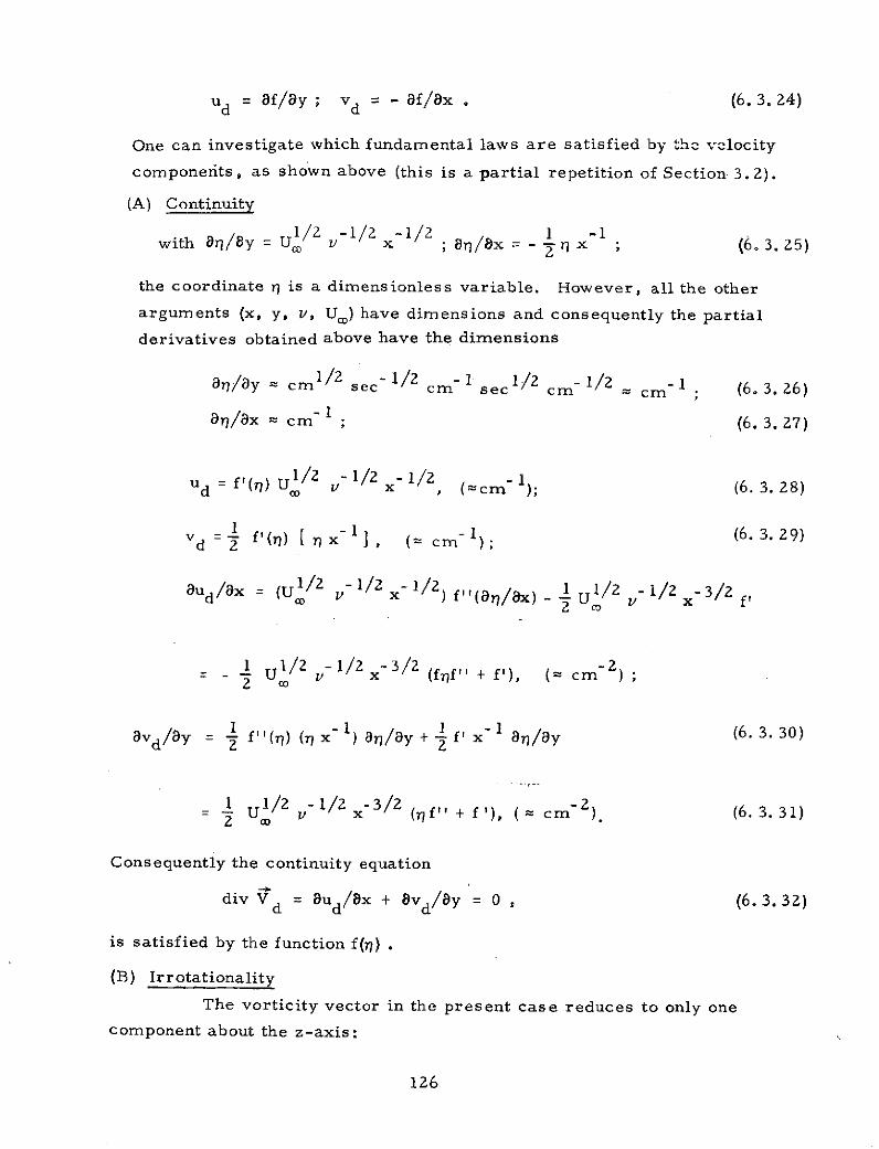
ud = f/Oy ; v d = - f/x . (6.3. 24)
One can investigate which fundamental laws are satisfied by the velocity
componerits, as shown above (this is a partial repetition of Section 3.2).
(A) Continuity
1/2 -1/2 -1/2 1 -1with Or?/8y = Ul v x ; a/Ox = - x ; (6.3. 25)
the coordinate Yr is a dimensionless variable. However, all the other
arguments (x, y, v, Uo) have dimensions and consequently the partial
derivatives obtained above have the dimensions
/y sec- 1/2 cm- 1sec 1/2 c-1/2 cm- 1 (6.3. 26)
Orn/Ox = cm- 1 (6. 3. 27)
d = '(7) U1/2 - 1/2 x- 1/2, (=cm- 1); (6. 3. 28)
vd l '() I r x- , cm1 (6. 3. 29)
aud/ax = (U 1/2 x-/2 1/2) f (a1/x) U 1/2 - x- 3/2 f,
1 1/2 1/2 3/o -- U 1/2 1/2 - 3/2 (fyf'' + f'), ( = cm ) ;
2 co
ad f "() ( x- 1) an/ay + I f ' x- I ar/ay (6. 3. 30)
1 /a 1/2 3/2 , -
= U1 vu-1 x-3/2 (f + f '), (= cm )2 (6. 3. 31)
Consequently the continuity equation
div Vd = 8ud/8x + 8vd/8y = 0 , (6.3.32)
is satisfied by the function f() .
(B) Irrotationality
The vorticity vector in the present case reduces to only onecomponent about the z-axis:
126

dz curl 1 - (6.3. 33)Wdz curl wd - (avd/ax - aud/aY)
Starting with Equations (6. 3. 32) and (6. 3. 30), one gets
S/ax 2 -2 3 -2 1 2 -1 -3aVd/x = - ~ r x - 4f'Cx = - 4 fy Uv x
3 1/2 - 1/2 -5/2-- f yU v- x
(= cm - ) ; (6.3. 34)
-1 -1 -2aUd/ay = U v x "(Z cm ) (6.3. 35)
This implies that:
dz (vd/8x - aud/ay) 0 ( cm-2) (6.3.36)
-2
where both terms have dimensions cm-2 and are not equal to zero. The
value of wdz was calculated at 2430 points with the following results:
-2the values oscillate around the numbers in cm ;
-0.4151 x 10 11; -0.8896 x 10 ; -0.6866 x 10⁻²⁵
-0.8440 x 10 27 (6.3.37)
-28 -2 8 -29-0. 8708 x 10 ; -0. 6727 x 10 ; -0.8937 x 10 29 (6.3.38)
-27The reader is reminded that the Planck No. is - 10 (.). Thus
in the laminar boundary layer, there appear vortexes with the values of
Wd of the order of the Planck number. Up to now, this fact was unnoticed
and quite clearly was never noticed by Prandtl and his followers.
In general, it is difficult, if not impossible, to locate in the
literature the definition of the vortex strength or of the vortex strength
distribution. The definition, listed below, is taken from Samaras: "Assume
an incompressible vortex-free velocity field without any volume source
intensity; for such a source-free vortex velocity field, the volume distri-
bution of vortices may be calculated from the vortex potential V . Samarasb.P
assumes that the circumferential velocity vector, v c , can be calculated in
the following manner:
v = rot V ; (6.3.39)c p
w = rot rot V = rot v ; (6.3.40)p c
127

2 -1where the vortex potential V has dimensions = cm sec
PReturning now to the problem of vortex characteristics according
to Howarth (p. 158):
2 -12 1 r v = K, K = cm sec (6.3.41)
it will be shown below that the variable K is equivalent to the vortex
potential V (Samaras). In Equation (6. 3. 41) the velocity vector v is
the speed along a streamline of radius r. The streamlines in two-
dimensional vortex flow are circles with their centers on the straight
axis, with the speed constant along any streamline. The motion is irro-
tational if the circulation has the same value, K, along every streamline.
Assuming that the circulation is equal to the vortex strength distribution
in volume or in area, Equation (6. 3. 41),and that the values used are those
calculated before, one gets the equation for wz:
Wz = (v/8x - au/8y) , (6. 3. 42)
or
d (8 d/8x - Bud/ay) , (6.3.43)dz = 8d d
which may better describe the problem under consideration. One can write
V = (u, v) (i u, j v) ; (6.3.44)
u = UC f'(Yl), (= cm sec - ) ; (6.3.45)
1 1/2 1/2 -1/2v (1/2 U/ x/2 (f' - f) (; cm secl); (6.3.46)
where (ud, Vd) may be substituted for (u,v). Suppose the motion is simply
a rotation with angular velocity:
= il + W2 + k 3 ; (6.3.47)
about an axis through the origin; moreover, let:
R = ix + j y + k z, (6.3.48)
be the vector from the origin to a point P(x,y,z); then the velocity at P
in such a rotation is:
S= x R; (6.3.49)
128

Sjk
U = 1 x R = ¢1 W2 W
x y z
= ( 2 z - 3 y) j 3 x - W) + k(w y-wx). (6.3.50)
T,he velocity vector U, Equation (6. 3. 50), corresponds to the velocity
vector v in Equation (6. 3.41). Using Equation (6. 3. 40), one canwrite
the vectors U and v (in the first approximation):
rot - rot U; U = i U + j U 2 + k U 3 ; (6. 3. 51)
U W2 z - 3 y; U2 w3x - z; U3 ly - 2x; (6.3.52)
U a 3 U 2 U aU a 3 u aU U IrotU Vx U ( - ) j + ( y ) ; (6.3. 53)
where the vortex strength distribution in volume or in area is denoted by:
-1)1 = vortex strength distribution in volume or in area (; sec-1)7(6. 3. 54)
In the above derivation one has to assume that d is constant (at least
temporarily). Then one gets for the boundary layer along an infinitely
long flat plate.
Vx U (v/8x - Ou/8y);
I C -1 (v/Ox - u/ay), (- sec- )7 2
where C must have dimensions of cm in order to be in agreement with
the concept of "circulation K" used in the Howarth sense, Equation (6. 3. 41).
If, in place of the components (u,v) one uses the components (ud, Vd), then
the dimensions of the constant C must be properly adjusted. In the problem
under consideration, one can observe that K in Howarth's approach corre-
sponds to V in Samara's approach;
K V . (6.3. 57)
From the discussion presented above, one can notice that the variable
129

1-Sw, Equation (6. 3.54), must be multiplied by the area (= cm ) in order
for one to be able to incorporate this variable into the idea of the entity2 -1
termed the vortex potential function, V , (= cm sec ). Continuingp
the present example, it is proposed that the vortex potential function,
V , Equation (6.3.57), contains a uniformly distributed vortex strengthp
(a hypothetical case) and that consequently one can write:
1- ~ 2Vp = K = C 2-w , C = cm (or any other properly chosen parameter),
(6. 3. 58)
and that from Equation (6. 3. 54) and Equation (6. 3. 58) one gets:
1 -. 2 -ZT r v =- C w ; C 1 x cm ; v = vd . (6.3.59)
Equation (6. 3. 59) was put on a computer to calculate the value of "r" at
2430 points of the boundary layer. The results are discussed below where
the values used are v = vd, w = dzThe following remark is in order:"The components of the velocity
vector, U, can be evaluated using the quantity 0, Equation (6. 3. 50). From
Equation (6. 3. 59) it is seen that components of U were assumed to be equal
to u and v, and it was further assumed that laminar flow components are
composed of small arcs of vortexes (SI). This was done deliberately, since
the investigator believes that "laminar" flow does not exist in viscous
fluids. A streamline is composed of small arcs of vortexes existing in
any viscous fluid flow, visibly unobservable and unmeasurable by macro-
scopic test devices. The vortexes are of dimensions approaching to the
value of the Planck constant."
A second remark which should be made is as follows: 'Past and
present literature contains very little, if any, information on such topics
as: calculations, operations, and manipulations dealing with the "vortex
potential". In particular, the manner of calculating the circumferential
velocity vector from the vortex potential is of primary importance,
since the curl and not the gradient is responsible for the main asDects inthe appearance of turbulence and for its results in both the microscopic
(unobservable) and macroscopic (observable) sense. From the numerical
data obtained by the writer, one could observe that the results of the
calculations show clearly that the values of r at high values of 7 = 8. 4 to
130
8.8, are relatively small. As an example, for = 8.4 to 8.8, r = -0.9089
x 10- 15 to r = -0. 2292 x 10 1 5 , r in cm. Actually, the increase in the
thickness of the boundary layer is due to the vertical motion in the layer,
which, in turn, is due to the vorticity and viscosity phenomena. These
phenomena become weak at the very large values of rl. When all of the
phenomena mentioned above become weak, then the graph of the
horizontal velocity component, u = f', becomes more flat and more
horizontal, the radius of the vortexes becomes small and the flow in the
boundary layer becomes more laminar. "
Summarizing, it has been proved above that,beyond any doubt,
"laminar" flow in the "laminar" boundary layer contains invisible vortexes
and vortex lines, and the flow is not "laminar" at all. The movement of
the layers of the fluid medium takes place by means of a "rolling" of the
layers of the medium on invisible "rolls" of vortex lines. This idea is
not a new one and the voices of other authors on the rolling phenomenon
appearing in layers of a viscous medium have been cited. The (Glauert, D. 100)
investigator has attempted to calculate the radii of vortexes, and in general
it can be said that it appears that at the front of the boundary layer, the
radius in question is very large. The larger the distance (measured along
the flat plate from the leading edge of the flat plate in the direction of the
flow), the smaller the radii of the vortexes become, dropping down to
a value comparable to the Planck constant. This implies that, at the
leading edge and at the front of the flat plate and of the boundary layer,
the "layers" of the fluid medium are "rolling" on big rolls, on big vortexes
in the medium (due to viscosity effects). Intuitively, such a geometric
interpretation of the physical phenomenon in question seems to make
sense. With increasing distance, when the first impulse of the incoming
flow becomes smaller, the boundary layer becomes better organized, the
"rollers" become smaller, their number increases when their size de-
creases, until finally the radius of the rollers reaches the length comparable
to the magnitude of the Planck constant. Since the Planck constant is
one of the characteristic quantities in the theory of quantum mechanics
(and naturally of wave mechanics),the following physical picture emerges
as the final conclusion of the foregoing reasoning. Up to now, the field
of fluid dynamics and mechanics was treated from the macroscopic point
of view, as a field belonging to the domain of the Newtonian mechanics,
131

whereas this research has demonstrated beyond any doubt that the formalism
and the operations in the field of the macroscopic fluid dynamics and
mechanics based on the Newtonian mechanics stands to profit by employing
concepts involving the Planck constant, which means the application of
microscopic methods of quantum mechanics. In this technique, a great
number of microscopic instrumentation and test devices are urgently
needed for application to fluid dynamics.
To be better acquainted with the influence of the disturbances
upon the stream lines (parabolas in the present case), various cases of
disturbances are considered below. These cases are put in form of
plots included in this report. The problem of disturbances (variations)
superimposed upon the function f' (r) was attacked and the results plotted
exactly according to the results obtained by Prandtl-Blasius and tabulated
in Schlichting's work:
I n) u-1 Y 1/2 - 1/2 - 1/2Cf) u = y U - x (6.3.60)
1I'( C f I if' + (f' - f) f.']
+_1 (U- I vx-)[rf,(rlT7 + rf'-f) + (r7f'-f)(3l'f" + lf')]} ; (6.3.61)
f' (r?) + H (rl) = disturbed f' (Yr) . (6.3.62)
Without a loss of generality the terms containing f"' are neglected due to
the fact that f' may not be tabulated (is not tabulated in Schlichting's work).
The function H' (rl) is calculated and its value is superimposed upon
the function f' (rI), and the sum is automatically plotted. The constant
Cad d is a parametric constant.
The parabolas plotted in the diagrams discussed above actually
appear at each point of the curve H' (q) or at each point of the sum of curves,
f'(rl) + H'(Y)). The parabolas appear, theoretically, at a number of
points of the curve [f'(n) + H'(1) ] . They are visibly unobservable
but the streamlines, after perturbations, even in stationary (steady)
conditions, intersect one another. The number of points of intersections
in the disturbed laminar flow and in the stationary conditions is very large.
When a fluid particle moves along one and the same streamline and next
meets another streamline, it must adjust itself to the conditions prevailing
on the "other" streamline. Among other things, it must adjust itself to the
132

direction of the velocity vector existing along the "new" streamline. This
requires a change in the direction of the motion of the fluid particle (in
the stationary conditions). As a result, at the points of intersections of
streamlines, there appears a rotation phenomenon which is one of the
most characteristic, if not the most characteristic physical feature of
all the phenomena accompanying the physical appearance of the disturbance
such as turbulence. On a film of turbulence one can clearly see the particle
clusters of the fluid medium which move and rotate.
6.4. Disturbance in the Thermal Boundary Layer
This section discusses the problem of the disturbances in the
thermal boundary layer. The concept of the dimensionless temperature
distribution presented non-dimensionally in the equation below serves as
the starting point (see Thermal Boundary Layers in Forced Flow,
Schlichting, p. 311):
- I 1 1(T - T,)(Tw - T) = [ 1 - E b(P)] 1 (r,P) + E 2E ,P);
for illustrative purposes, various approximative assumptions were already
made in Equation (6.4.1). Consequently, the use of various approximations
seems to be fully justified. In Equation (6.4. 1) the following approximation
values of the product are applied:
E b = 6, 4, 2, 0, -2, -4 ; (6.4.2)
as taken from Schlichting'' book, p. 316. The value of the coefficient
b is equal to:
b(P) = 8 2 (0,P) = 2(0); (6.4.3)
with P- 1; which results in
(0 ) = 1 - f' (0) = 1 , f' (0) = 0 ; (6.4.4)
The chosen value of P = 1 represents an approximation. The value of the
function 0 1(YT) is assumed always to be equal to (1 - f'(7)) for P = i, even
133

if the value of P (the Prandtl Number) oscillates and take on values
close to 1. The value of the dimensionless Eckert Number appearing in
the last term in Equation (6. 4. 1) can be calculated as
E = U [ g C (T - Tj] - (6, 4. 5)
where the values of the other coefficients are
-2g = 978.05 cm sec ;
c = specific heat at constant pressure of air = 0. 242.
The value of the coefficient c is taken from Stewart "Physics," p. 252.p
As is well-known, the definition of the specific heat is as follows, Stewart,
p. 252: "The specific heat of a gas at constant pressure is numerically
equal to the number of calories required to change the temperature of
1 gram of the gas 1 degree centigrade."
From the equivalence of the work and heat, it is known that
1 cal = 4. 18 x 107 ergs, Stewart, p. 247, with the erg defined in the
c. g. s. system in the well-known manner as: 1 erg is the work done when
a force of 1 dyne is exerted on a body and there is a displacement of 1
centimeter in the direction of the force. British units, Btu(ib deg F) -1
can also be used. Without going into too many details of a fundamental
nature, the results of the calculations of Equation (6.4. 1) are presented
where the following value for the coefficient b is taken into account:
b = 0. 835 (Schlichting, p. 316, Fig. 14. 12); P = 1. (6.4. 6)
If one prefers to use the values of the coefficient c in terms of
Btu units, a short table of the thermal properties of substances
as prepared by E. Schmidt as referenced is given in the work
of Schlichting, Table 14. 1, p. 294. Equation (6.4. 1) is
expressed in the dimensionless units, since the composite coordinate r
is a dimensionless coordinate and the factor-coefficients (E • b) and E
are dimensionless parameters. Next, the results of the calculations
of Equation (6.4. 1) were plotted for various values of the parametric
coefficients (E * b), and E, b = 0.835, P = 1. These curves are denoted
as the "thermal laminar flow or undisturbed flow curves" and will be
subjected as a first step to small disturbances by means of superimposing
134

upon them "small disturbances" in form of the first derivative of the
function appearing on the right-hand side of Equation (6. 4. 1). The function-1 -
under consideration is [ Equation (6. 4. 1) with (T - T)(T w - Tco)
T(r)] :
T(4) = [ 1 - E b(P)] 01 (,P) + E e(,P), (6.4.7)
where the symbols used denote
E = Eckert Number from Equation (6. 4. 5) which is dimensionless);
b = dimensionless coefficient from Equation (6. 4. 6);
P = Prandtl Number (dimensionless), P = 1;
P=va g -1 k-1 (6.4.8)
0() = (1 - f'(N)) with P = 1 ; (6.4.9)
a ( ) = (1 - f'2(n)) with P = 1 . (6.4. 10)
Then one gets by differentiation:
01(n) = -f"(l) with P = 1 ; (6.4.11)
01(2) = - 2 f' f" with P = 1 . (6.4. 12)
The coefficients in Equation (6.4.7) are kept unchanged during the process
of differentiation and consequently the derivative of the function T(77) has
the form:
T'() = [ 1 - E b(P)] (-f"() + E [ - f ff" ()] , (6.4. 13)
with P always being equal to unity. Another form of Equation
(6.4.13) is:
T() = - "(){[ 1 -E * b(P)] + E 2 f'() } , (6.4.14)
where P = 1, b = 0.835, E * b takes on the sequence of values in
Equation (6.4.2), and E is calculated each time from the assumed
and chosen value of the product (E * b). Equation (6.4. 7) presents
a family of curves plotted as functions of the coordinate r7.
These are called the "undisturbed" curves on which are superimposed
the first order disturbances in the form of Equation (6. 4. 14).
135

Consequently, the final curves which are plotted and enclosed in this
report as Appendix are the curves:
Ttot T() + T() ; (6.4.15)
curve T(Y) + disturbance T'(Y) = Ttot(n) ; (6.4. 16)
Equation (6.4.7) + Equation (6.4. 14) = Equation (6.4. 15).
These curves are presented for various values of the parameters
E and b. Each plot represents a curve such as f'(u), T(a), T(Y) + T'(r), etc.,
which is always a function of the coordinate rj in the ir-space. Along these
curves (functions of rj) a rectangular coordinate system (x,y) moves such
that the x-axis is always located horizontally and the y axis is always
located vertically. Moreover, the horizontal axis, x, is sometimes
plotted on the logarithmic scale whereas the vertical axis, y, is plotted
on ordinary (linear) scale. For each point rl on any curve in the a-space
there corresponds a parabola since 7r = constant y x 1/2. Each time the
parabola is located in the moving Cartesian coordinate system (x,y).
These parabolas represent the streamlines in the thermal layer in the
physical (x,y) space. Each point on any curve, T(), as a function of the
coordinate r), is associated with the parabola in the physical space (x,y),
and is located in the moving Cartesian coordinate system in (x,y) space.
Obviously, these parabolas, i. e., their branches, intersect each other
with the points of intersections clearly seen on the computer plotted
diagrams.
In general, one can distinguish three cases of parabolas from
S = y x/2 constant ; (6.4. 17)
constant = /2 -1/2 (6.4. 18)
1st case: r = positive; x = positive; x- = positive; y = positive;
2nd case: q = positive; x -1/2 = negative; y = negative;
3rd case: r = positive; one branch of the parabola has:
x = positive; x = positive; y = positive;
the other branch of the parabola has:
x-1/2 = negative; y = negative .
The third case seems to be highly hypothetical but still, physically, it
136

seems to be possible and even practical. The path, streamline, of a
particle consists of two parts of a parabola; one branch of the parabola
is directed in one direction, another branch of the parabola is directed
in another direction. When two branches of two different parabolas meet
at a vertex which is common to both branches and common to both
parabolas, the common vertex is located exactly at the point r1, which is
the origin of the running coordinate system (x,y) and consequently is
located at the point (0,0) of both parabolas. The various branches of
various parabolas intersect. The final path of a mass particle is the
curve connecting all the intersecting points.
At the points of the intersections of the two parabolas, i.e. , the
streamlines, the particles of the medium have to pass from one stream-
line to another. Since, in stationary conditions, the tangent to a stream-
line at any point gives us the direction of the velocity of the motion of
the particle , the points of intersections of two streamlines are
equivalent to the physical phenomenon of passing the particle from one
streamline to another. Since the intersections usually take place at an
angle, which is different from 00 or 1800, the intersections of streamlines
(parabolas) causes an abrupt change of the paths of particles as a result
of sudden rotation (macroscopically at a point). The rotations of particles
are perhaps the most characteristic macroscopic optical phenomena of
disturbed (turbulence) flow under physical observation. This report
presents a certain number of computer plotted diagrams in the fl-space
and of the corresponding parabolas in the moving (x,y) Cartesian
coordinate systems referring to the cases investigated; i. e. , the
disturbed flows in the three cases:
(a) boundary layer along an infinitely long flat plate;
(b) thermal boundary layer in forced flow;
(c) flow in the boundary layer around circular cylinder.
6. 5. Computer - Analyzed - Geometrical - Graphical Plottering -Step-by-Step - Successive - Iterative - Approximation - Quantum -
Theoretic - Method
From the formalistic point of view, the technique used in the
present work involve the most modern aspects of the computer-age era:
computer -analyzed, geometrical, graphical plottering, step-by-step,
successive -iterative - approximation, quantum. theoretic methods.
137

These methods are used in all the problems attacked in the present work,
including the problem of C. A. T. A brief summary of the entire formalism
and of the particular steps is demonstrated below on the simple problem
of Prandtl -Blasius boundary layer flow along an infinitely long flat plate.
(1) As the first point one may discuss the dimensionless variable
y = Y(x,y). From the structure of this function one can see that the con-
dition Yr = constant and dy = 0 leads to the relation y = y(x). The constant
in the relation Yr = constant has to be treated as a parametric constant
(temporarily fixed). For various values of rl one obtains a family of
parabolas in the space (plane) of (x,y) coordinates, depending on
various values of Yr = constant.
(2) The function f = f(rj), representing a function of one (composite)
variable, Y is given and is available in the tabular form. It is a dimension-
less stream function. It is a differentiable function and there exist tables
of the derivatives of this function up to the second order, i.e. , f, f', f".
Due to the fact that f represents the dimensionless stream function, the
condition f = constant represents the family of streamlines, the above
constant being a parametric constant, i. e. , a step-wise varying constant.
In reality, the first derivate, df/dy = f', represent the velocity, i. e. ,-1
f' = u Uc I. The entire effort of Prandtl and Blasius was spent to get
this result. They (wrongly) believed that their effort gave them the
"laminar, " one-directional flow. These functions are "undisturbed"
functions.
(3) The next point is to introduce disturbances superimposed upon
the function f. The following function is considered and plotted as function
of T?:
f(t); H(n)
The function of H(r7) is used as function of Yr in the intervals of-6 2 -1
rl = 0. 2 from r = 0. O to Y = 8. 8, with v = 14. 9 x 10 met sec
U = 200 km hour-1 .
(4) The next point refers to the first derivative of the function f
and disturbances superimposed upon f'. This means that the functions
f' and H' are plotted as functions of r7. The function f' is
a dimensionless horizontal velocity component function and the function
H' is a dimensionless disturbance function superimposed upon the velocity
138

f'. Since the function f'" was not calculated and tabulated, it was
neglected (without a loss of generality).
(5) The next step in the proposed procedure is to pass from the
space of the ,r-variable to the two-dimensional space of two independent
variables (x,y). Since Yr = r(x,y):-1 -1 1/2
? = Y(x,y) = y(U v x ) ,
any point Yr = fixed (constant), corresponds to a parabola. The following
sequence of operations may be proposed:
(6) The curve f'(r) + H'(r) is plotted as a function of r). This
operation is done automatically (by the plotter).
(7) A sequence of points is chosen on the plotted curve f'(Y) + H'(Y)
for rl having the following values: rj = 0.1, 0.2, 0.3, 0.4, and so on,
up to i = 8.8.
(8) Keeping r = fixed (temporarily), each q is associated with a
parabola passing through the chosen Y1.
(9) Thus one can visualize a running, (x,y), Cartesian coordinate
system along the curve f'(l) + H'(Y). The axes of this running coordinate
system are directed in the same directions: the x-axis is always directed
horizontally, the y-axis is always directed vertically.
(10) These parabolas, passing through each point Yr-fixed, represent
the streamlines in the (x-y) plane inside the boundary layer in question
subject to some disturbances due to the superposition of the term containing
the factor U x Vx U.
(11) Each point Yl = fixed is associated with two parabolas.
(i) one parabola with the corresponding point in infinity
is located to the right. This parabola has both its "arms"
directed to the right.
(ii) The second parabola with both its "arms" directed to
the left.
(12) Both parabolas, discussed above, are plotted for each point
of the curve:
f'()) + H'(r) = f'(Yr) + disturbance function (r)
(13) Both parabolas represent the streamlines in the physical
space (x-y plane) in the laminar boundary layer in question, in which
there were introduced some disturbances due to the superposition
139

upon the laminar boundary layer (in Prandtl -Blasius formulation) the
additional term v w (full or only a part of it). Intersection points determinez
the zig-zag pattern.
(14) The flow above the infinitely long flat plate takes place from
the left to the right. The streamlines torn to pieces in the running (x-y)
Cartesian coordinate system show clearly the zig-zag path of particles
which prior were moving along the streamlines in question. The zig-zag
path is due to the introduction of the curl (U x Vx U) into the flow pattern.
(15) The zig-zag path pattern obtained represents (in the first
approximation) the first break-through with regard to the geometry of the
turbulence phenomenon. One can notice the characteristic sharp corners
at the intersections of parabolas which, obviously, exist actually when the
particles of the fluid in question pass from one parabola to another: i.e.,
from one streamline to another. One has to keep in mind that these sharp
corners exist in a realistic flow condition (as in the present case). Such
sharp corners are, perhaps, the most characteristic features of the
phenomenon of turbulence as seen from any oscillogram of turbulence.
(16) The plots of the streamlines are done entirely automatically
by the computer and are enclosed in the present report.
(17) The plots use two coordinate systems: The system of Y) where
the horizontal axis rl is traced in the normal (linear) scale. The same is
true for the vertical axis on which the function f'(r) + H'(r) is measured;
the second coordinate system is the running coordinate system. It is a
rectangular (Cartesian) coordinate system with the x-axis directed
horizontally and the y-axis directed vertically. This system moves on
the f'(Y) + H'(rl) curve and at each point of it the value of the t-coordinate
is temporarily fixed, to enable one to plot the two parabolas. The horizontal
x-axis is sometimes plotted to make it more adaptable to the existing
conditions in the logarithmic scale. The vertical axis or the y-axis has
the normal, linear scale.
(18) The plots of the streamlines, subject to the small variation
(disturbance) refer sometimes only to the part of the circulation vector
appearing in the problem; i.e., only a /a x(v 2 ).
140
(19) Usually the entire vorticity component wz = (8 v/8 x - 8 u/8 y)
was taken into account in the present report.
(20) The results obtained as presented and discussed above, seem
to be the first of this kind of break-through in the analytical representation
of the phenomenon of turbulence. The investigator presented his ideas
to Professor von Karmdn in Paris in June of 1955 while on sabbatical
leave. von Karm/n was very much interested in these ideas. At the
time the investigator was unable to pursue these ideas because of the
lack of high speed computers.
(21) The investigator is convinced that the results obtained in the
present research is primarily possible through application of the tool
of quantum mechanics. The use of the deterministic, classical mechanics
would not allow for as deep a penetration into the fundamentals of the
flow of a viscous fluid as has been possible with the application of the
quantum field theoretic methods because the wave mechanics equation
is a linear equation.
(22) To justify partly the statement expressed in point (21) above ,
the author quotes a sentence from a private letter received from Dr. Ottmar
Wehrman in Fokker -Werke, West Germany: "For your information I am
preparing a paper on quantized vortex sheddig and measurement of vortex
phenomena behind very small cylinders. These measurements indicate
a critical quantized wave length of 2. 78 x 10 2 cm for the vortex street
formation."
(23) The author has indicated many times that his evaluation of
the possible radii of the vortices in the laminar boundary layer along an
infinitely long flat plate oscillate around a value in the neighborhood of-27
the Planck constant; i.e., around 10 and are visually unobservable.
(24) The report includes plots of the curves f'(r), H'(r), the
geometrical sum [f'(4) + H'()], two parabolas at each point n = constant,
intersection points of the streamlines (parabolas), and the zig-zag
patterns representing, from the physical point of view, the paths of the
particles. From the geometrical point of view the zig-zag path consists
of small parts of streamlines located between the intersection points.
141

Thus a particle moves along one streamline, meets' another streamline at
the intersection point, rotates at this point, passes from one streamline
onto another streamline, moves for a short distance along the second
streamline, up to the intersection point with a third streamline, rotates
at the intersection point, passes along the third streamline, and so on.
Graphically, the zig-zag patterns, obtained in a purely analytical-
geometrical -graphical manner in the present report, are similar to
oscillograms of turbulence obtained from measurements (windtunnel
in the wake of a cylinder and other geometrical forms) obtained in a
purely physical manner by means of oscillographs. The first iterative
approximation using the analogy between the analysis and geometry on
one side and the physical experimental tests on the other, presents very
good agreement. The next steps to be discussed below should involve
the correlation phenomena between two and more clusters of elementary
particles, the results of the interference phenomena due to the inter -
particle force action and the resonance phenomena; the results can be
superimposed upon one another due to the fact that the systems are linear.
(25) The points (1) to (24), presented above, are the first steps
which have to be undertaken by the investigator to solve the type of pro-
blems discussed. Due to the linearity of the applied equation and the
possibility of summing of any arbitrary number of steps, the main
emphasis is put upon the step-by-step successive iteration procedure,
computer work, computer -plottering, plots, graphs, graphical represen-
tation of the results, and the interpretation of the graphical results. The
number of points, (1) to (24), discussed above, is very modest. They
serve only as the preparation for the main problem, to be attacked in
the future, i.e., the problem of C.A.T. There the number of points
will be much greater due to the fact that the writer has to take into account
such phenomena like the interference between the clusters grouped around
electrons, interference and correlation phenomena among them, resonance
phenomena and many other items. Each such an additional plhenomenon
142
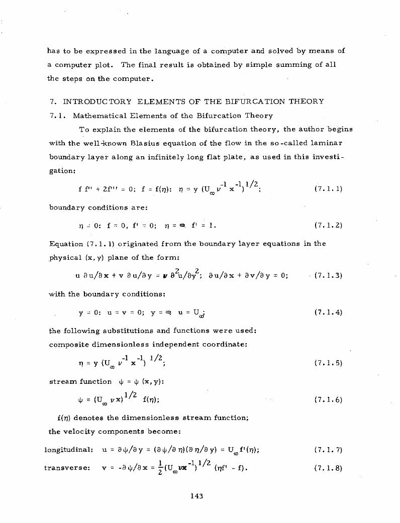
has to be expressed in the language of a computer and solved by means of
a computer plot. The final result is obtained by simple summing of all
the steps on the computer.
7. INTRODUCTORY ELEMENTS OF THE BIFURCATION THEORY
7. 1. Mathematical Elements of the Bifurcation Theory
To explain the elements of the bifurcation theory, the author begins
with the well-known Blasius equation of the flow in the so-called laminar
boundary layer along an infinitely long flat plate, as used in this investi-
gation:
-1 -1 1/2f f" + 2f"' = 0; f = f(r): = y (U x ) ; (7.1.1)
boundary conditions are:
= 0: f = 0, f' = 0; r = f' = 1. (7.1.2)
Equation (7. 1. 1) originated from the boundary layer equations in the
physical (x, y) plane of the form:
u a x + u/ x v u/y = 8u/y; a u/a x + 8 v/a y = 0; (7.1.3)
with the boundary conditions:
y = 0: u = v = 0; y = C u = Ucd (7. 1.4)
the following substitutions and functions were used:
composite dimensionless independent coordinate:
S= y (U v x ) ; (7. 1.5)
stream function L = q (x,y):
1/2¢ = (U, vx) / f(Y); (7. 1.6)
f(i7) denotes the dimensionless stream function;
the velocity components become:
longitudinal: u = 8 /8 y = (a /a )(a n/a y) = Um f' (); (7.1. 7)
transverse: v = -a8 /8x = (U X ) 1/2f' - f). (7. 1.8)
143

Equation for the stream function f(rj), Equation (1.7. 1) is an
ordinary nonlinear differential equation in the function f(T) of the third
order. The three-boundary conditions (7.1.2) are, therefore, sufficient
to determine the solution completely. Blasius especially looked for the
function f'(t7), Equation (7. 1.7), due to the fact that the function f'(t)
expresses physically in the two-dimensional (x,y) plane (the reader
has to keep in mind that the xy-plane is the physical plane of the actual
real flow) the horizontal velocity component in the laminar boundary layer
along an infinitely long flat plate. Moreover, the three available boundary
conditions, Equation (7. 1.2) and Equation (7. 1.4), refer specifically to
the horizontal velocity component, u, usually expressed in the dimensionless-1
form, uU .
Equation (7. 1. 1) is a highly nonlinear ordinary equation in the
function f(i) and its ordinary derivatives; expressed, as it is, in the form
of Equation (7. 1. 1) it obviously may have more than one solution. One
of these solutions should satisfy the required boundary conditions given in
the forms of Equation (7. 1.2) and Equation (7. 1.4). Boundary conditions
expressed in form of Equation (7. 1.4) refer to the physical (x,y) plane
of the actual, real, macroscopic flow. The solution which satisfies the
boundary condition given in Equation (7. 1.2) and in Equation (7.1.4) is-1
the well-known Blasius' solution, uU = f'(r). All the other possibleco
solutions of Equation (7.1.1) do not need to satisfy the required boundary
conditions expressed in form of Equation (7.1.2) and/or in the form of
Equation (7. 1. 4).
One of the possible solutions of Equation (7. 1. 1) (not necessarily
satisfying the required boundary conditions in the form of Equation (7. 1.2))
may be chosen in the form:
fl( ) = f'() = 1; f 1"() = 0; f 1"'( ) = 0; (7.1.9)
in such case, Equation (7.1.1) takes the form:
f l ( r) x fl"( 7 ) + 2fl"'() = 7 x 0 + 2 x 0 = 0, (7.1.10)
144
which is correct and consequently the function fl(n) = Y satisfies Equation
(7. 1.1).
Equation (7. 1.5) defines the association between the two spaces:
(a) the physical space having two coordinate systems, (x, y) and (b) the
"intermediary" nr-space, having only one coordinate, rl, as its independent
variable. Thus it may be considered to act as the "transformation
equation" between the physical (x, y) space and the intermediary i-space.
Equation (7. 1.5), as it now stands, contains the square root from the-1
quantity x. Under the definition of the "rationalization" process, one
means the process of operations which may allow one to get rid of the
terms containing square root, third root and similar, briefly, the terms
which are not "rational" terms. The "rationalization" procedure, when
applied to Equation (7. 1.5), is equivalent to the process of squaring of
Equation (7.1.5) and results in:
2 2 -1 -1y TUvx ; (7.1.11)
As a peculiar feature of the nonlinear equations to which class of
equations Equation (7. 1. 1) belongs, one may notice that Equation (7. 1. 5) ,
after the "rationalization" procedure,does not satisfy Equation (7.1.1).
In reality, let:
f ( ) = r 2; f '(7) = 2r; f 2 "(n) = 2; f z2 '(n) = 0; (7.1.12)
Equation (7. 1.1) now takes the form:
f 2 (n) f 2 "(7) + 2f2 '"() = Y7 x 2 + 2 x 0 = 0, (7.1.13)
which obviously cannot be true, unless n = 0.
The fact that the function fl (r) = 27 satisfies Equation (7. 1. 1), and
the same function after the rationalization procedure, f 2 (7) = T ,does not
satisfy the same equation, Equation (7. 1. 1), is due to the peculiar
properties of the nonlinear equation, Equation (7. 1.1). As is well-known,
due to the lack of the knowledge of the characteristic properties of the
nonlinear differential equations (both ordinary and partial), only one state-
ment can be made which is definitely true: if the equation in question is
145

definitely not a linear one, then it is (and may be called) nonlinear.
The function 4 was introduced above, called the dimensional stream1/21/21/2 -1/2 1/2 1/2 -1/2 2 -1
function (v x 1/2 f() = cm sec cm cm sec = cm sec
and the function f(t), called the dimensionless stream function.
According to the fundamental concepts of the fluid dynamics theory,
the condition that a stream function is equal to a constant defines a
stream line (or a set of stream lines). This implies that the following
equation must be true:
fl(17) = Y = constant; or rationalized r77 = constant; (7.1.14)
or
2 2 -l1 -1S= y (U v ) x = constant, (7.1.15)
determines a set of stream lines. Equation (7.1.15), i.e.:
2 -l -1y (U O ) x = constant, (7. 1.16)
in the space of the Cartesian coordinates, (x,y), represent a parabola:
2 -1y = constant U vx = 4 a x; (7.1.17)
-14a = constant U V, (7.1.18)
the vertex of the parabola is at the origin of the coordinate system
(x = 0, y = 0); if a > 0, the parabola is opened to the right; if a < 0
it opens to the left. The parabola opened to the left can be obtained
from the parabola opened to the right by a rotation of the parabola by
1800 around the vertical y-axis. Assume that a mass particle is
located at the origin of the coordinate Cartesian (x,y) system. The
origin of the system is located at any arbitrary point on the Blasius-1
curve, f'(0) = uU - , function of r. Through the point (x = 0, y = 0)
one can trace two parabolas -- one opened to the right and another
opened to the left. Each parabola represents a possible streamline
of the mass particle located at the origin. If a particle at a certain
moment would become a subject of small oscillations around the origin
of the (x,y) system, it would oscillate on infinitesimal or small finite
146

arcs of one of the two possible parabolas--one opened to the right
or another opened to the left. Thus, in general, through any point-1
on the Blasius curve f'(r) = uU , chosen temporarily, as the origin
of the Cartesian coordinate system (x,y), there pass three curves:-1
(a) the Blasius curve, f'(7) = uU0 ; (b) a parabola (a streamline),
fl() = = constant, or r7 = constant, whose vertex is located at the
origin of the (x,y) coordinate system and which is opened to the right;
and (c) a second parabola (streamline) whose vertex is located also
at the origin of the (x,y) coordinate system but which is opened to
the left. All three curves, treated from the analytical point of view
as functions (f'(7) = uU -1 fl() = constant, or before the rationali-2 2 -l -1
zation process, 7= y (U v ) = constant), satisfy the fundamental
nonlinear ordinary equation f f" + 2 f'" = 0, or fl f" + 2 fll, = 0,
proposed and derived in 1908 by Blasius.
The above presentation is a good introduction to the necessity
of application at this point the elements of the Bifurcation Theory.
This will occupy the remaining part of this Section (see "Bifurcation
Theory and Nonlinear Eigenvalue Problems" edited by Joseph B. Keller
and Stuart Antman, New York University, Publisher, W. A. Benjamin,
Inc., New York, 1969, pp. XI to XIV).
By a term "a nonlinear eigenvalue problem" one means the
problem of finding appropriate solutions (more than one) of a nonlinear
equation of the form:
F (u,X)= 0. (7.1.19)
In Equation (7.1.19) the symbol F denotes a nonlinear operator, depending
upon the parameter X , which operates on the unknown function or vector u.
Obviously, one of the first questions a reader can ask and which has to be
answered is the following one: suppose that the numerical value of the
parameter X is given, then the question is, does Equation (7. 1. 19) have
in this case any solution u ? If it does, the next question arises as to
how many solutions it has, and then how this number of solutions varies
147

with X . Of a particular interest in that respect is the process of bifur-
cation whereby a given solution of (7.1.19) splits into two or more solutions
as X passes through a critical value X , called a bifurcation point. The
main problem is to determine the properties of the solutions and how they
depend upon X.
To illustrate bifurcation, let it consider the linear eigenvalue
problem of the form:
Lu = u. (7.1.20)
Here L is a linear operator operating upon vectors u in some
normed linear space and X is a real number (definitions of norm, measure,
space, measure space, metric space, measurable space, and others can
be found in Paul R. Halmos ' "Measure Theory", University of Chicago,
D. Van Nostrand Comp., Inc., Princeton, N. J., 1956). Consider, at
first, that the parameter X in Equation (7.1.20) can take any arbitrary
value equal to any real number. Then, obviously, for every real number
value of X, there is a solution of Equation (7. 1.20) equal to:
u = 0. (7.1.21)
Geometrically, this solution can be represented in the following manner:
Assume a two-dimensional space and a Cartesian coordinate system--
on the horizontal axis one will measure the values of numerical values
of the parameter X (X -axis), on the vertical axis one will measure the
value of the solution, Equation (7.1.21). Under the term "norm of a
vector" (see John W. Dettman, "Mathematical Methods in Physics and
Engineering", McGraw-Hill Book Company, New York, 1969, p. 27),
one usually means the length of the vector, i.e., for the vector u:
The norm is:
IIu II (u, /2 (7.1.22)
The norm of a vector is usually assumed to represent the value
of the vector if and when the vector is a solution of an equation such as
Equations (7.1.20) and (7.1.22). The author makes a second assumption
148

that on the vertical y -axis of the two -dimensional Cartesian coordinate
system considered above, one will measure the norm, 11 ul, of the
vector u representing the solution of Equation (7.1.20). Figure 1
represents, in general, a two-dimensional space, (X , II u If). In the
present case, II ul = 0 is a solution. As the next problem, let us assume
that there is a sequence of eigenvalues, X1' < < 3 < .... , and a
corresponding sequence of normalized eigenfunctions ul, u2, u 3 , .*.,
such that both sequences satisfy the linear equation, Equation (7.1.20):
L u. X . u.; I u. H 1; j = 1, 2, 3, ..... , (7.1.23)3 3 J
If c is any real number, other possible solutions of Equation (7. 1.20)
are given by:
u = c u., j = 1, 2, 3, ...... (7.1.24)
The norm of the solution (7.1.23) is clearly jI u = 0, while the norm of
the solution of Equation (7. 1.24) is II u II = c. A graph of the norms of
these solutions is shown in Figure 1. As the figure shows, the solution
u = 0 splits into two branches at each of the eigenvalues X., located on
the horizontal X -axis. Therefore, the points u = 0, X = X., are designated
as the "bifurcation points" of the linear problem given in Equation
(7. 1.20).
By turn, the author may briefly present the main characteristic
features of the nonlinear eigenvalue problem, Equation (7. 1. 19), which
has Equation (7.1.20) as its linearization. An illustrative plot of u
versus X (called the response diagram) is shown on Figure 2. It
demonstrates the following behavior:
(i) The branches emanating from the eigenvalues of the linear
problem are curved.
(ii) There may be no branch emanating from an eigenvalue of the
linearized problem. This occurs at X 2 in Figure 2.
(iii) There may be several branches emanating from an eigenvalue
of the linearized problem as from X 3 in Figure 2.
149

(iv) There may be a secondary bifurcation as on the branch from X 4*(v) The branches from distinct eigenvalues of the linearized problem
may be connected. This happens with the branch through X 5 and
X .(vi) There may be branches that do not emanate from the eigenvalues
of the linearized problem, such as the branch C.
Concrete examples of such response diagrams occur throughout the entire
field of the bifurcation theory. In each case some but not necessarily all
of these phenomena occur. In the diagrams a quantity which can be
either positive or negative is often plotted in place of [I u II.
7. 2. Application of the Bifurcation Theory
At the present time, one can notice in world literature a tendency
to apply very strong methods to understand better and possibly to solve
the problem of turbulence in fluids (liquids and gases). Others use the
bifurcation theory and other attacks on the nonlinear eigenvalue problems.
These are very difficult and little known fields of the modern applied
mathematics. As is clearly seen from Section 7. 1, the results of the
application of the Bifurcation Theory, from the geometrical-graphical
point of view, are usually represented in form of loops, multiple points
and multiply-connected particle -paths. The multiply-connected paths
often have their origins located at one point on the original curve. As-1
an example, the author can mention the curve f'(7) = u U , discussed
thoroughly in this report. It represents the horizontal velocity componenet
in the laminar boundary layer flow along an infinitely long flat plate.
Through any arbitrarily chosen point on this curve there pass two stream-
lines, r2 = constant. Consequently, at any point on the curve f'() =
-1uU there meet the three curves discussed above.
The parabolas represent the two possible streamlines, (72 = constant),
of a mass -point located initially at the chosen point r = constant on the
curve f'(i7). Consequently, the reader may immediately recognize an
important characteristic feature of the bifurcation theory, namely the
multiple points located on any curve which represents a possible solution
150

I1 uI
2 3 4 5 6
Figure 1.
1 X2 3 X4 5 6
Figure 2.
151

of a nonlinear equation. The Blasius equation of the laminar boundary
layer along an infinitely long flat plate, f f" + 2 f"' = 0, f = f(0), is a
highly nonlinear ordinary differential equation in one independent composite
variable I = rl (x,y). Consequently. the bifurcation theory may be
successfully applied to this equation. The appearance of the multiple
points on various curves of the higher order (in the present case of the
third order) is obviously a natural phenomenon. The set of streamlines
constructed in this work was presented above in detail by means of
computer plots. Streamlines traced at various points intersect each
other and the pieces of streamlines between the intersection points form
zig-zag patterns. The zig-zag patterns represent the final paths of mass
particles in the flow under consideration. Due to the intersections of
parabolas, there appear the "parabolic loops" in the pattern of the flow.
In general, the appearance of various kinds of "loops" like circular,
elliptical, parabolic, is one of the most characteristic features of any
disturbed flow of gases and liquids. The turbulent flow belongs to the
cathegory of disturbed flow systems. The pictures of the surfaces of
fluids in the status of turbulence show very clearly the existence of loops
of various kinds.
It seems appropriate now for the author to explain in detail the
technique used in this research. Equation,derived by Blasius, f f" +
2 f"' = 0 is a highly nonlinear equation. The use of very complicated
power expansion of infinite series, asymptotic expansion for large values
of r1, plus a construction of a common joint point of the series (at which-1
both series furnish the same value of f'() = uU -) for the horizontal
velocity component in the laminar boundary layer along an infinitely long
flat plate. Of course this solution satisfies the two required boundary
conditions in the flow in question, i.e.,
r) = 0: f = 0, f' = 0; 17 = w, f' = i. (7.2.1)
I have proposed two other solutions of this equation in form of two parabolas-1
passing through each point located on the Blasius curve, f'(rl) = uU :
152

one parabola opens to the right and another parabola to the left. The
two parabolas do not satisfy the required boundary condtions, Equation
(7.2. 1), but they satisfy the Blasius equation. The parabolas, traced
by computer plotter at successive points of the Blasius curve, f'(r7) =
function of r7, intersect each other at many points. This gives the origin
to the parabolic loops and to the zig-zag pattern which is perfectly
analogous to the oscillograms of turbulence in wind tunnel and in the wake
of a cylinder. The results obtained by the author with the use of the
computer plotter refer to one single moment (with no time interval taken
into account).
One may propose a comparison of these results obtained from two
sources. In such a manner one can venture a statement that the geometric-
graphical zig-zag plots obtained by means of computer plotters (this is
the mathematical side of the technique) represent in the first approximation
the oscillograms of turbulence (or of a similar disturbed flow domain)
obtained by means of oscillographs (this is the physical side of the technique).
In such a manner the author succeeded to obtain in a first approximation
some sort of agreement between physics and mathematics. The reason
why this technique was chosen is simple: at the present status of applied
mathematics the writer was unable to apply directly the bifurcation theory
in a purely deterministic sense, to find more than one solution of the
nonlinear Blasius equation, and to obtain the sought parabolic (or elliptic
or circular or any other) loops which are so characteristic for turbulent
domain. Solutions which cannot be obtained by means of purely deter -
ministic techniques can be approximated by means of probabilistic
geometrical -graphical plots obtained by computer -plotters and wave
(quantum) mechanics. In case the first approximative solution of the
disturbed (turbulent) flow, as described above, would not be sufficiently
accurate, one may try to use higher order approximations. One of these
would be to describe the zig-zag pattern obtained above by means of
Fourier analysis. A different problem is to learn how to read and to
understand the zig-zag patterns obtained above and how to associate
153

them with the physical, natural problems which are under investigation
now (like C.A.T.). This will be done separately.
7.3. References to Section 7
For the sake of convenience to the reader, collected below are
some references containing information on the subject of the Bifurcation
Theory and its application to the theory of turbulence. In particular,
one can refer to the following authors, papers and books: Keller and
Antman, Marsdeen, Ruelle and Takens, and Vainberg and Trenogin.
8. LAMINAR FLOW
8. 1. Macroscopic Laminar Flow
The investigation begins with macroscopic laminar flow, observable
by means of macroscopic instrumentation, with the well-known statement
of W. Heisenberg (1948) who said that, "''contrary to the common belief,
it is the so-called macroscopic laminar flow, and not the turbulent flow,
which needs a deep scientific investigation. " It has been demonstrated
in this investigation that (macroscopic) laminar flow is not at all laminar
(in the full meaning of this definition). It possesses vortexes, vortex
lines and vortex tubes, and is closer to turbulent flow than to laminar
flow in the full meaning of these definitions from the macroscopic point
of view. Laminar flow possesses vortexes whose radii are very small.
Below a certain length of the radius the vortexes in a fluid medium cannot
be seen and visually observed.
This indicates that the present day division of the field of fluid
dynamics (laminar and turbulent flows) should be abandoned in favor of
a more realistic division: macroscopically visible and observable
flow and only microscopically observable flow. Below a certain length
of the radius, the vortexes cannot be seen by naked human eye. Special
techniques and instrumentation must be used in order to notice, to
investigate and to test the phenomenon of turbulence. Another aspect
which should be mentioned is approach to fluid dynamics from the side
154

of wave mechanics. This field usually refers to very small elements
and masses like electrons. To make the approach more practical the
writer proposes the approximation in the sense that in place of an
electron the writer considers a cluster of mass particles gathered
around the electron and guided by it. The classical, deterministic
fluid dynamics begins with the concept of mass density of a fluid in3
question, i.e., mass per cm in standard atmospheric conditiors on
the earth. This is a large amount of mass. If necessary, they take
into consideration the rarefied gas domain, where the amount of mass3.
per cm is appropriately smaller. The approach to fluid dynamics
with the use of the wave mechanics (often called quantum fluid dynamics)
begins with the concept of electron, next passes to the concept of the
cluster of particles gathered around the electron. In such a manner
one may approach to the concept of mass density by increasing the amount
of the mass of the cluster of mass particles gathered around the electron.
The main reasons for using the quantum fluid (or wave) mechanics approach
and not the deterministic, classical fluid dynamics approach are purely
practical. In some problems (but not all) the wave mechanics gives
much better results than the deterministic fluid dynamics. The deter-
ministic, classical fluid dynamics uses as the fundamental system of
equations either the spatial form of the Euler's momentum equation
(for inviscid, ideal fluids) or the Navier -Stokes equation (for viscous
and heat-conducting fluids). Both equations are highly nonlinear and
thus cannot be solved exactly (excluding some special simple cases).
The wave mechanics (or quantum mechanics) approach uses as the
fundamental system the Schroedinger wave equation. This is a linear
equation. A system of such equations and their results can be summed
and/or multiplied by constants.
In the last few decades the quantum theoretic methods in statistical
physics became the most successful techniques used in solving many
practical problems.
155

8.2. Association Between Two Domains: Wave Mechanics (Microscopic)
and Classical, Deterministic (Macroscopic) Fluid Dynamics
The reader is asked to give special attention to the way of achieving
a passage from the micro-domain to the macro-domain. The passage
from the microscopic domain of the validity of the quantum theory, of
the Planck constant ( - 10-27 ). to the macroscopic domain of the validity
of the ordinary mechanics (classical or even diabatic) where the variables,
like the density of the medium are measured, tested and subjected to
the observable, macroscopic experimentation is achieved in a direct
way. Namely, each, however small it may be, particle of the medium
is subjected directly to the action of the external force fields in the same
sense as it is accomplished in the ordinary, macroscopic mechanics
but through the use of the Avogadro's Law and Number. It states that
if N is the number of molecules in the gas, V the volume of the gas, then
the ratio N/V has the same value for different gases at the same p and
T (pressure and temperature). Other forms of the Avogadro's law are:
The number of molecules in a kilomole, namely, the mass in kilograms
of the substance which is equal numerically to its molecular weight is
constant; or, the number of molecules present in equal volumes of gases
at the same pressure and temperature are equal. The number of
particles per unit volume can be found from
n = (p /A) Na
where:
p = density of the gaseous species (kg/m3
A = atomic weight; Na = the Avogadro number 60.2472 x
1025 molecules per kilomole.
Other details of this nature are known from primary courses in physics.
Fundamentally, the method applied in this research follows the
ideas expressed in "Feynman diagrams". The "basic advantage of the
Feynman diagram technique lies in its intuitive character. Operating
with one-particle concepts, one can use the technique to determine the
structure of any approximation. Next, one can write down the required
156

expressions with the aid of correspondence rules. These new methods
make it possible not only to solve a large number of problems which
did not yield to the old formulation of the theory, but also to obtain many
new relations of a general character. At present, these are the most
powerful and effective methods available in quantum statistics."
(A. A. Abrikosov, L. P. Gorkov, I. E. Dzyaloshinski, Methods of
Quantum Field Theory in Statistical Physics, translated by Richard A.
Silverman, Prentice -Hall, Inc., Englewood Cliffs, N. J., p. V, 1964).
The next practical problem to be explained is the problem of a
successful extension of quantum theory to the domain of nuclear dimensions.
The writer quotes from D. Bohm, "Quantum Theory, " Prentice Hall,
1964, p. 627: "We state that quantum theory has actually evolved in
such a way that it implies the need for a new concept or the relation
between large scale and small scale properties of a given system.
Between others, one may discuss two aspects of this new concept:
1. Quantum theory presupposes a classical level and the correctness
of classical concepts in describing this level. 2. The classically definite
aspects of large scale systems cannot be deduced from the quantum-
mechanical relationships of assumed small-scale elements. Instead,
classical definiteness and quantum potentialities complement each other
in providing a complete description of the system as a whole. Although
these ideas are only implicit in the present form of the quantum theory,
we wish to suggest here in a speculative way that the successful extension
of quantum theory to the domain of nuclear dimensions may perhaps in-
troduce more explicitly the idea that the nature of what can exist at the
nuclear level depends to some extent on the macroscopic environment. In
this connection it was shown that the definition of small scale properties
of a system is possible only as a result of interaction with large scale
systems undergoing irreversible processes. In line with the above
suggestion, we propose also that irreversible processes taking place
in the large scale environment may also have to appear explicitly in
the fundamental equations describing phenomena at the nuclear level."
157

The part of the suggestion of D. Bohm, which was followed by
this investigator literally (almost word by word) is underlined. Instead
of upgrading the quantum theory fundamental equations and results from
the microscopic, quantum level upward to the level of the macroscopic,
observable test-measurable fluid dynamics, the investigator
down-graded the equations of Prandtl, Blasius (and others), of the
Navier-Stokes class of the macroscopic level, origin and nature,
observable, test-measurable-character down to the level of the quantum
theory of the microscopic nature and character. This was done directly,
without creation of any special idea of the quantum theory philosophy.
In the notion of the Planck K-Number, which represents some sort
of hypothetical generalization of the Planck constant, the most important
variable quantity seems to be the density of the fluid medium in
question, but expressed in terms of units of gram-mass. The process
of the transformation of the density of a medium from one system of
units to another (and vice versa) is very simple and was discussed
in Section 2.2.
8.3. Step-By-Step Successive Iterative Method
The fundamental philosophy of the method is proposed by John
von Neumann in his "Mathematische Grundlagen der Quanten-Mechanik, "
Springer Verlag, Berlin, 1932. One operates in the finite phase-space
with (p,q) coordinates. The phenomena under consideration refer to a
medium without any dissipation; no friction, no viscosity, and no heat
conduction take place. Thus one treats only the ideal fluid system.
The fundamental equation used is the Schroedinger wave equation, the
formal mathematics used is the probability theory, the sought results
are presented in the form of the mean values. The domain of the opera-
tions is a finite one; in the case of a necessity of extending it up to
infinity, one could use a conjecture on the extending the John von
Neumann's philiosophy, theory and proofs to function spaces and to
fields discussed above. Practically, fluid dynamics at this point will
give solutions to problems involving the domains of ideal (perfect)
fluids. In this domain the gradient and the curl can be treated separately
158
and independently, and the results of all of the operations and manipula-
tions can be added due to the concept of linearity.
In the next step, one superposes upon the domain of an ideal fluid
the viscosity and heat conduction (dissipation, internal transfer of
momentum, and of energy) phenomena. This means that there takes
place a transformation of the ideal fluid into a real one, possessing
the coefficients of viscosity, and of heat conductivity; the fluid may be
subject to some chemical reactions, thermal reactions, and so on.
Any time a new phenomenon of the physical nature appears in the ob-
servation, one can use the results from the previous phase of the research
and superpose upon it the new, additional characteristic properties of
the medium in question. To achieve a great precision and accuracy,
one may apply the successive iteration procedure; as it is well-known,
according to the Seidel hypothesis (or Seidel-Gauss) such a process.is
a convergent one (in a given interval) or at least an asymptotic one.'
At this point, actually, the adiabatic flow of the medium is transferred
into a diabatic flow.
The above method of the successive steps can cover the domains
of an ideal fluid, real fluid, incompressible media, compressible media,
viscous, or heat conductive fluids. Next one can also include subsonic
domain, transonic flow, supersonic flow, or hypersonic domain. The
entire region of the flows in the region of the kinetic theory of gases can
be treated in this manner. To close the list of all of the possibilities in
the field of fluid dynamics, one should mention the flow of electro-
magneto-conducting fluids, plasma fluid dynamics, ion gas dynamics
and others.
The question of validity of the approach to fluid dynamics problems
from the point of view of wave mechanics is discussed very thoroughly.
At certain temperature above T O (absolute zero) there appears the
phenomenon of superfluidity, of the mixture of two fluids, and finally
a phase transition at X -point, below which the superfluid motion is
159

possible, but above which the superfluid motion is no longer possible and
the hydrodynamics of the Bose fluid does not differ from the ordinary
hydrodynamics. The definition of small-scale properties of a system is
possible only as a result of interaction with large-scale systems which
are always undergoing irreversible processes. In line with the suggestion
of physicists one may propose that irreversible processes taking place in
the large-scale environment may also have to appear explicitly in the
fundamental equations describing phenomena at the nuclear level. This
fundamental concept is used in this investigation, where the Navier-Stokes
equations are expressed by means of the modified form of the wave
equation (Schroedinger) with the mass of the electron "m". Next, they
are "elevated" from the level of the Planck constant to the level of the
Planck K-number which involves the inertial force terms (numerator) in
the Reynolds number. The above proposition could be referred to as the
quantum-mechanical model of the fluid dynamics with the proper contribution
paid to Feynman technique, correspondence rules, and Madelung's proposition.
8.4. Diabatic Flow
The concept of the diabatic flow was developed by the National
Aeronautics and Space Administration in the United States during and
after the second World War (- 1946). According to this concept the flow
phenomena with heat addition and dissipation can be treated in almost the
same manner as the flow phenomena in the classical dissipationless do-
mains. By a proper organization of the sequence of events, even the time
variation can be taken into account. In each sub-domain one can apply
the notion of the friction and of dissipative (negative) forces such as
viscosity and heat conduction. Upon treating the dynamic system in
question in a manner similar to that in the classical flow system, one
passes from one domain to another, and the coefficients (of viscosity and
heat conductivity) are changed correspondingly; i. e., they are different
from those in the previous domain. This sort of a step-by-step variation
of the coefficients and of the analysis by means of the use of the "destruc -
tive forces" and of the force potentials allows one to use practically the
formalism and the methods of classical mechanics in the domain of
160

"diabatic" (as contrary to "adiabatic") flow phenomena. The diabatic
flow concept will be used primarily in the domains where there appear
the friction (viscosity), heat conduction and analogous phenomena. Names
associated with the concept of the diabatic flow are those of Hicks, Was-
serman, Montgomery and others in N.A.S.A.
More remarks and details on the subject of the association between
two domains, quantum mechanics (microscopic) and classical, determin-
istic (macroscopic) mechanics, including the notion of diabatic flow, are
contained below.
8. 5. True Nature of the Laminar Flow
Several writers, such as W. Heisenberg, H. Dryden, and others
(see list of references, particularly in Dryden's work, 1951), have called
attention to the necessity of the investigation of the true nature of the
laminar flow in viscous fluids. Quoted below is the opinion of Dryden
about Heisenberg's point of view:
The Mechanics of Turbulent Flow
The past few years have seen the introduction of new conceptsand considerable progress in studying the mechanics of turbulent flow.The interest taken by such eminent physicists as Heisenberg, Chandra-sekhar, Onsager, von Weizsacker, and the great activity of von Karman,Batchelor, Townsend, and others have been major factors in thesedevelopments which can only be sketched in rough outline.
This sketch may be prefaced by a quotation from Heisenberg, asfollows:
A few remarks may be added with regard to the physicalpicture of turbulence presented in the recent papers. In theearlier years one thought that turbulence was caused byviscosity. This seemed to be true since without viscositythe liquid could theoretically perform all the classicallaminar motions, where the liquid glides along the walls; itis only through the viscosity that rotational motions areproduced near the walls. At present we know that it isalmost the other way round. The liquid without frictionis a system with an infinite number of degrees of freedom.It is extremely improbable that only those few degrees offreedom which a laminar motion represents should beexcited. As soon as one puts energy into a liquid without
161
friction, this energy will be distributed among all degreesof freedom, and what finally results is a certain equilibriumdistribution, corresponding to the Maxwellian distribution ingases. It is the viscosity that reduces the number of degreesof freedom, since it damps very quickly all motions in the
very small eddies. Therefore only through viscosity is alaminar motion at all possible. Turbulence is an essentiallystatistical problem of the same type as one meets instatistical mechanics, since it is the problem of distributionof energy among a very large number of degrees of freedom.
This is indeed a refreshing and stimulating reversal of our usual
point of view. It is not turbulence but laminar motion that requiresexplanation.
The writer begins with the conventional approach to the notion of
stream function and streamlines in the "laminar" boundary layer along
an infinitely long flat plate as formulated by Blasius:
1/2 - -1 1/2)(V = (vx U ) f () = (U v x y; (8.5.1)
1 1 /2 -1/2 1/a /a x ) x f () + ( U / f' () a/a x; (8.5.2)
a /ax =-2 (VUx) - f' ()) = -v, (8. 5.3)
with:
an/ax (- -1 (8.5.4)
a4/8ay = (8 4/8 ) (8 Or/ y) = U f' () = u ; (8.5.5)
from the definition of streamlines:
4 = constant; dLP = (8 4/8 x) d x + (8 4/8 y) dy = 0 ; (8.5.6)
one gets:
-vdx + udy = 0; v/u = dy/dx, (8.5.7)
as the equation of streamlines in the "laminar" flow.
As the next step the writer selects various admissible forms of
the function f(17):
(a) f(t) = 7; = (vx U / (U v x ) y = U oy; (8.5.8)
162

condition for streamlines, 4 = constant:
dP = (3 4/ x) d x + (a 4/@ y) dy = 0 + U dy 0= , (8. 5.9)
gives, after the integration:
U y = constant, (8. 5. 10)
as the equation of the streamlines parallel to the x-axis; the fundamental
equation:
ff" + 2 f, = 0, f = ; f' = 1; f" = f'" = 0, (8.5.11)
is satisfied; the boundary conditions:
0 = O: f = 0, f' 0 O; r7 = cn f' = i, (8.5.12)
may be considered to be satisfied, at least conjecturably;
2 1/2 -1 -1 2(b) f(T) =r ; (vxU I (U v x ) y constant; (8.5.13)
1/2 -1 -1 2 3/2 -1/2 -1/2 2( VxU (U x ) y = U x y = constant, (8.5.14)
represent one possible equation of streamlines. Another possible set of
streamlines may be obtained from the conditioni:
w lZP = (vxU 1) = C 1 C = C 17 = C 3 = constant;
1/2 -1 -1 2 2(vx U/ C1 = constant; (U v x )y = = C 2; (8.5.15)
2 -1 -12r = C /C = (U v x ) y = C = constant;
still another possible set of streamlines can be obtained from the squaring
of Equation (8. 5. 14), after rationalization:
3 -1 -1 4U v x y = constant; (8.5.16)
the writer will concentrate on the last Equation (8. 5. 15); this is an
equation of a parabola of the second degree:
2 -1 -1y =C U vx = 4ax; C U v = 4 a; (8.5.17)
1 -1a= Cz U ;
4 2163
163

this is an equation of a parabola with vertex at the origin of the two -
coordinate system (x,y), and focus at (a, 0). The parabola opens to the
right if a > 0, and opens to the left if a < 0. Since both C 1 and C 2 may
be simultaneously positive or both negative, the parabolas Equation
(8.5.17), passing through any point ri (or - 2) fixed on the curve f'(r)
may be opened to the right or to the left. As is already known, the
writer traces through each point (17 = fixed) two such parabolas, having
common vertex at the origin of the two -coordinate (x, y) system (r =
temporarily fixed). Let it verify the relation between the function:
f(0) = n2; f'(r) = 2l; f"(4) = 2; f'"(I) = 0, (8.5.18)
and the equation:
f f" + 2 f 0"=0; = 0: f =0; f' = 0; r =C: f' =1; (8.5.19)
the function r2 does not satisfy Equation (8. 5. 19) except at the 71 = 0;
boundary conditions are satisfied only at Y7 = 0.
All the groups of streamlines originated at each point (7 fixed)
located on the curve f'(7) form the set of bifurcation curves, and bifurca-
tion loops belonging and attached to the curve f'(r). The curve f'(Y) =
-iuU-1 belongs to the set of bifurcation curves as the base of the points
7 = fixed. The streamlines of all the groups intersect each other. At
the points of intersections the moving particles change the streamlines
and pass from one streamline to another. They are subject to a rotation
and to change in the direction of motion. An observer may have the im-
pression that they move "aimlessly", but always inside the main stream
of flow which follows the direction of the pressure gradient. All these
aspects are responsible for the disordered outlook of a turbulent fluid,
like the surface of a turbulent fluid spread with aluminium powder (see
plate No. 15).
The technique of streamlines with intersection points and with
the resulting zig-zag paths is applied by the writer to the well-known
laminar flow curve f'(rl) = uU -1 (Blasius, 1908). The resulting zig-zag
164

paths are clearly seen on plates No. 21 and No. 31. In plate No. 21, at2
each point 7 = fixed (or 12 = fixed), the parabolas are plotted by the
automatic computer-plotter according to the second Equation (8. 5. 15):
-1 -1 2 2 -1(U v x )y = C ; y = C ( vU )x; (8.5.20)S2 2 O
the numerical value of C is assumed to be equal to the numerical value
of 0Z at each considered point. This means that C 2 is assumed to be a
parametric constant running along the curve f' (1) and not an absolute
constant.2
In plate No. 31, different values in y = 4 ax defining the parabolas,
representing the streamlines, are used. The use of Equations (8. 5. 3),
(8.5. 5), (8. 5.7), and the square of Equation (8. 5.7) give the following-1)2
expression for ( ) , Equation (8. 5.7):
(vu -1 [nf'(n) - f (n) /{(xU u- 1 ) [f'(n)]2 } , (8.5. 21)
and similarly, in Equation (8. 5. 17), the expression for 4a:
4a = [nf'(n) f(r)]2/ {(U - l )[ f ' rf ( n 2) } (8.5.22)
it can be seen that there are little differences between the zig-zag paths
in plates No. 21 and No. 31. The curve f'(Y?) = uU -1 was verified experi-
mentally with the use of macroscopic experimental devices by several
outstanding scientists during a period of several decades. The writer's
results prove without any doubt that the flow in the boundary layer along
an infinitely long flat plate, which is laminar from the macroscopic
(observable by naked human eye) point of view, is turbulent from the
microscopic point of view (the existence of zig-zag paths). This conjecture
is in full agreement with the existence of the vortexes and vortex tubes in
the laminar boundary layer. The radii of these vortex tubes are very small.
They are of the order of 10-20 in the cgs - system. In the laminar flow
region the vortex tubes are nicely ordered. The thin laminae of the fluid
are moving on "rollers" over one another. Prandt -Tietjens describe
this phenomenon in the following manner -- there exist two radically
different kinds of flow; considering, for instance, the flow through a
165
glass tube, using water in which small particles are suspended, it is
seen that most often the particles of fluid do not move in paths parallel
to the walls of the tube but flow through in a very irregular manner.
Besides the principal motion in the direction of the axis of the tube,
secondary motions perpendicular to the axis can be observed. This
kind of flow is called "turbulent" flow. The majority of cases of fluid
flow are of this kind. There is a certain small velocity at which the
individual particles of fluid move regularly in paths parallel to the walls
of the tube. This is the second kind of flow referred to, commonly called
"laminar flow" (Prandtl-Tietjens, p. 14). In the present section the
writer has proven without doubt that the so-called macroscopic, laminar
flow is turbulent from the microscopic point of view. Here lies the first
partial answer to the Heisenberg point of view. "As soon as one puts
energy into a liquid, this energy will be distributed among all degrees of
freedom, resulting finally in an equilibrium (Maxwellian) distribution in
gases. It is the viscosity that reduces the number of degrees of freedom,
since it damps very quickly all motions in the very small eddies. There-
fore only through viscosity is a laminar motion at all possible."
From plates No. 21 and No. 31, one can notice that the laminar
flow curve f'(l) is actually a mean value curve of the zig-zag path traced
(hypothetically) by a particle or a cluster of particles. And vice versa --
suppose that a particle or a cluster of particles follows the zig-zag paths
clearly seen on plates No. 21 and No. 31. If, in each of these cases,
one would trace the mean value path between the valleys and the hills of
the zig-zag paths, one would obtain the curve f'(~). The mean values
have to be calculated according to the rules of the probability calculus.
Thus, this reasoning serves again as another partial explanation of the
Heisenberg approach to the notion of the macroscopic laminar flow.
Namely, in a viscous flow along an infinitely long flat plate there is an
infinite number of degrees of freedom. The viscosity reduces the number
of degrees of freedom and leaves, as undamped, these oscillating clusters
of particles which result as the zig-zag paths seen in Plates No. 21 and
166

No. 31. Next, if one would trace the mean value path between the valleys
and the hills of the zig-zag path in each of these two cases (following the
rules of the probability calculus), one would obtain the curve f'(TI).
Therefore, one could define a laminar motion as a mean value path f' (7)
of the cluster of particles which follow the zig-zag paths of streamlines
(broken to pieces) exactly according to the patterns found in plates No. 21
and No. 31.
The next problem and question which can be proposed in connection
with the notion of turbulence and turbulent flow, with Heisenberg's definition
of the laminar flow, with an infinite number of degrees of freedom, with
the above suggested proposition of the laminar motion as a mean value
path of a cluster of particles which follow the zig-zag paths of broken-to-
pieces-streamlines, and with others, is the following: Is it possible to
propose and to discuss some typical and characteristic cases from the
infinite number of degrees of freedom proposed in the Heisenberg's
approach? This is an important question since in the phenomenon of
C.A. T. there appear to be some cases which can be included into the
class of typical degrees of freedom. The answer is a positive one, and
below the writer will attempt to list a few of the most typical degrees of
freedom. The reference system is assumed to be the classical, three-
dimensional, Cartesian system of coordinates (x,y,z).
8. 6. Elementary Notions of Particle Kinetics
Before continuing the discussion of the laminar flow, it may be of
some value to review the particle kinetics of fluids. The motion of waves
and groups of waves (mentioned below) refers to the motion of molecules
and atoms. The molecule is made up of atoms; the molecules of water
vapor, for example, is a cluster of two hydrogen atoms and one oxygen
atom. A substance that contains only atoms with identical chemical
properties is called an element, while one built of molecules that contain
atoms with different chemical properties is called a compound. Elements
' This section may be omitted.
167

smaller than the atom are the proton, the neutron, the electron, the meson,
and the positron. The proton has a positive charge of electricity and a
mass as large as that of the hydrogen atom; the neutron has no charge
and approximately the same mass as that of hydrogen atom; the electron
has a negative charge and a mass about 1/1850 of that of the proton;
the meson (sometimes called mesotron) has a charge of the same size
as that of the electron, may be either positive or negative, and has a
mass about 200 times that of an electron; the positron has a positive
charge and seems to have a mass about the same size as that of the
electron. All atoms have a dense core, or nucleus, surrounded by
electrons. The hydrogen atom, which is the simplest of all atoms, has
as its nucleus one proton, with an electron outside it. The more common
form of the helium atom has a nucleus with a mass about four times that
of the hydrogen nucleus, with two electrons outside the nucleus. Because
the nuclei of all atoms contain protons, they are positively charged;
in a normal atom there are always enough electrons surrounding the
nucleus to make the total negative charge on the electrons equal to the
positive charge on the nucleus.
The table included in this paper shows the probable structure of
the stable forms of a few of the simpler atoms. The two most important
quantities used in comparing different atoms are the mass of an atom and
the size of the electric charge on the nucleus. Since protons and neutrons
have approximately equal masses, and since the mass of an electron is
approximately negligible, the masses of the atoms are approximately
proportional to whole numbers. The "mass numbers" given in the table
are the nearest whole numbers to the exact value of the atomic masses.
In each case, as may be seen in the table, the mass number is equal to
the total number of protons and neutrons in the nucleus. Since the posi-
tive charge on a proton and the negative charge on an electron are
numerically equal, and since the total charge of an atom must be zero,
the number of electrons surrounding each nucleus must be equal to the
number of protons in the nucleus. The "atomic number" of an element
168
is equal to the number of electrons or to the number of protons in the
atom; it is proportional to the magnitude of the electric charge on the
nucleus. In a case where two kinds of elements have equal charges on
the nucleus and consequently the same atomic number, the elements
have identical chemical properties (which depend solely on the magnitude
of the electric charge which atoms carry) and cannot be distinguished
by any chemical process. Those atoms which have the same kind of
chemical properties and the same atomic number, though different
atomic masses, are called "isotopes".
Some most characteristic numbers are:-27
h = Planck' constant = 6. 55 x 10 ; cm gram sec;-27
m = mass of the electron = 0. 9107 x 10 gram;-24
mass of a hydrogen atom = 1.66 x 10 gram;
mass of the hydrogen molecule is twice that of the atom;
the number of molecules per cubic centimeter in a gas at
atmospheric pressure and 0 C is 2.69 x 10¹⁹ (see Stewart,
p. 191).
When considering and discussing the notion of the velocity, one
should refer to the so-called "group velocity" (Bohm, p. 64). The
"group velocity" denotes the speed of motion of a group of waves collected
together in the form of a packet. A wave packet comprises a group of
waves of slightly different wave lengths, with phases and amplitudes so
chosen that they interfer "constructively" over a small region of space,
outside of which they produce an amplitude that rapidly reduces to zero
as a result of a "destructive" interference. Further discussion concern-
ing the fundamental nature of matter and energy is omitted; the notion
of waves and of groups of waves mentioned above in the description of
a wave packet refers to the motion of atoms.
There is a distinction between the groups velocity and the "phase
velocity". The phase velocity is precisely the speed with which a point
of constant phase moves when w and k are defined. The symbols used
denote the following:
169

k denotes the wave vector
w = k c; c = velocity of light (8.6. 1)
frequency f = w(2) -1 = k c (Zr) =c (8.6.2)
X = wave length _ L; k kx k + kz ; c k
2ZrcL ( +12 +1 ) (8.6.3)
kx = 2L-x ; k = 2TL-1 y; kz 2rrL z (8.6.4)
Ix = Lk(2V)-1 ; 1 = Lk (21)- z = Lkz (2)-1
X =L = ( 2+ +y + 2 1/2. (8.6.5)
This sketchy information may be sufficient for the reader to com-
prehend the general ideas necessary to select the proper size and con-
sistency of the cluster of elements and molecules which may, and should,
be used in place of the mass of electrons in the Schroedinger equation
when passing from the operations in the micro -fluid dynamics (quantum
fluid dynamics) to the macro- or ordinary classical fluid dynamics.
All the above data are important when considering the true nature of the
so-called laminar flow in the macroscopic domain in the Prandtl-Blasius
sense.
8.7. Possible Degrees of Freedom'
The possible degrees of freedom in a system of particles repre-
senting a fluid (liquid or gas) can be divided into the groups listed below.
(1) The first group includes curves of one degree of freedom -- simple
curves like sin and cos, having mean value paths always along one of the
axes (x,y, z); vibrating, string, or oscillating, according to triangular
or similar shapes; and multi-triangular formations having multiple-knot
points. The mean value paths are always straight lines located on one
of the axes (x,y,z). Three-dimensional configurations can be decomposed
into three directions (x, y, z), expressed in the form of separate, single
wave functions, ,1(x), 4' 2 (y), or L3 (z) , and the results can be summarized.
Any other oscillatory phenomenon can be expressed geometrically in
an arbitrary form such as rectangle, trapezoid, pentagon, hexagon,
: This section may be omitted.
170
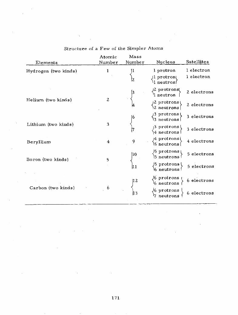
Structure of a Few of the Simpler Atoms
Atomic MassElements Number Number Nucleus Satellites
Hydrogen (two kinds) 1 1 1 protron 1 electron
1 protron 1 electron1 neutron
3Z protrons) 2 electrons1 neutron
Helium (two kinds) 2 2protrons
2 protrons electrons
Sneu protrons 3 electrons3 neutrons
Boron (two kinds) 35 protrons 5 electrons
4neutrons,
6 protrons
Carbon (two kinds) ons 6 electrons
7 neutrons
171

hexagram, or analogous. These geometrical forms should be located
above and below one of the axes, and the mean values should be located
on one of the axes. One can propose oscillatory motions constructed in
such a manner that the mean values are located on one of the curve-
linear axes (segment of a circular arc, say). The general rules of the
mean (verage) values in the probability calculus are well-known: the
average value of the position x = C P(x)xdx, P(x) = (x) (x); of any
function of x: T(x) = f:(x) f (x) t (x) dx, 4*(x) being complex conjugate;
LP has to be normalized, so that: fo 6dx = 1, or: JIA f c, ' , pdx = 1.
A being a suitable constant.
(2) The second group may contain whirls and vortexes of all kinds:
circular, elliptical, and spirals, both two- and three-dimensional.
(3) The third group of higher order degrees of freedom may involve
resonance phenomena between "n" oscillating clusters, n = 2, 3,......
(4) The fourth group may involve phenomena due to the intermolecular
forces and interference effects between the "n" oscillating clusters.
(5) The fifth group refers to the heat transfer phenomena. Using the
analogy between heat transfer, skin friction, and similarity theory, the
above cases of the interference and interaction between clusters of
particles may be investigated from the point of view of the transverse
transfer of momentum (viscosity phenomena) and of the transverse trans -
fer of energy (heat conduction phenomena).
In summary, clusters of particles taking the place of the electron
"m" in the Schroedinger equation are subject to various kinds of mechan-
ical-dynamic phenomena. Some are subject to the external force
gradient, some are subject to the heat (energy) action, and some are
subject to the expansion (density change) phenomena. Analytically, each
of the groups discussed above is expressed in terms of the Schroedinger
equation (linear), and the results are summed up.
Other writers sometimes divide the shape factors and the inter-
molecular forces which appear in non-ideal gases into different groups
172

than those discussed above. Thus chemistry proposes the divisions
listed below (as an example see The Properties of Gases and Liquids,
Robert C. Reid and Thomas K. Sherwood, McGraw-Hill Book Company,
1966, pp. 46-47):
Shape Factors and Intermolecular Forces. Molecules are not
point masses and may have many diverse shapes. Even simple spherical
atoms such as argon attract or repel other argon atoms, depending upon
the separation distance; in addition, at high pressures, the volume frac-
tion occupied by the atoms themselves may be significant. Molecules
behave in a similar way. The fact that real molecules have interacting
forces and finite molecular volumes is usually the most important reason
why the ideal gas law, pV = RT, is not obeyed.
Electrical Forces. Electrical forces of a permanent kind are
usually important only in so-called "polar" molecules. Nonpermanent
electrical forces, such as electric moments arising from the short-
lived perturbation of the electron positions during a collision or near
collision, are included above and are present in all real systems. These
forces are included in the potential-energy relationships between molecules.
Electrical forces, excluding hydrogen bonding, depend upon the
molecular dipole moment, the quadrupole and higher multipole moments,
and the polarizability.
Hydrogen Bonding. Hydrogen bonding between molecules usually
occurs in systems of a polar nature. Such forces are often considered
in the same category as electrical forces.
Quantum Effects. Quantum effects are important only in those
molecules where the translational-energy modes must be quantized;
such molecules as H 2 , He, and Ne at low temperatures are the only
ones which have significant quantum effects.
These four effects must be considered when methods are proposed
to describe the variation of the P-V-T behavior of a real gas from that
of an ideal gas.
In the particle kinetics of plasmas, the polarization force appears
173

during a collision of an electron and a neutral particle.
It should be realized that the polarization force is only one of the
many forces which act during a collision of an electron and a neutral
particle. Other forces which can be significant are listed as follows.
The value of r) in F -r-7-1 is also given when applicable.-5
(1) Repulsive polarization force, r = 4, proportional to r 5. To
allow for a screening distance r , we write a more correct2 22
polarization potential as V = -A /(r + r )p
(2) Attractive Coulomb force between electron and atomic nucleus,-2
1 = 1, proportional to r-2
(3) Repulsive force of the atomic electrons screening the nucleus --
not a simple power dependence. This can be obtained from
calculations by Hartree using his expression for the atomic
potential.
(4) Short-range repulsive exchange force, due to the exclusion (Pauli)
principle for particles of like spin. This force prevents the
spatial overlapping of the electron shells of the molecule and a
free electron.
(5) Other attraction forces may be important, such as the self-dipole
moment of polar molecules, where r = 2, the charge-induced
quadrupole term, and the London dispersion-energy term, both
with a potential which varies as r = 6.
In electron scattering by molecules, additional complications are
present which do not exist in electron-atom scattering. For molecules,
nearly elastic collisions can occur. In these collisions, the molecule may
be excited to higher rotational and vibrational states. In this case, the
entire spectrum of the target molecule is involved in the calculation.
Furthermore, for molecules, the potential is a function of angular direc-
tion as well as of distance r, since the potential in general is not
spherically symmetric.
174

9. OTHER POSSIBLE FORMS OF WAVE EQUATION AND PHYSIO-
LOGICAL ASPEC TS
9. 1. Schroedinger Equation
The wave equation is the linear equation, whereas the equations
of the classical, deterministic, macroscopic hydrodynamics are
usually nonlinear partial differential equations; this aspect seems to be
one of the greatesL advantages of using the Madelung's idea and of an
association of wave (quantum) mechanics with the macrodynamics
following Feynman's technique. One kind of the Schroedinger equation
is of the form of the amplitude equation
V2Po 8 m h- z(W-U)o = 0 ; (9. 1.1)
0 = o exp (i Z T W h - t) ; (9.1.2)
here the following notation is used:
b = wave function;
o = amplitude (function) ;
W = energy of the system;
U = potential energy of the system.
Often, Schroedinger equation may be used in the one-dimensional form:
d u/dx + 8 2 mh - (E-V) u = 0; u = u(x) ; (9.1.3)
where
V U = potential energy function;
E W = total energy = p2 (2 m)-1 + V ; (9.1.4)
p = momentum,
p2 (2 m) -1 = kinetic energy.
The Schroedinger equation may include the time; in this case it becomes
(another form of this equation):
2 2 -2 -1 _
V z - 8 2 m h U - i4w mh 8 = 0 (9. 1.5)175t
175

In general, one usually seeks a finite and continuous solution
for any equation in the domain in question. In the case of
the Schroedinger equation a solution is possibly only for
certain values of the total energy W. These values are called the
"eigenvalues" of W. The eigenvalues of W are the values of the energy
of the system in question, which the system possesses (or occupies) in
its "quantum states." These states may be established and confirmed
by means of electroscopic devices. To each eigenvalue of the Schroedinger
equation there belongs an "eigen-solution" of the Schroedinger equation;
such a solution should be "normalized" and multiplied by the "time factor"
exp (i Zw Wh-1t); put in such a form, the eigensolution--according to
Schroedinger (see Madelung, p. 322)--represents the phenomenon under
consideration and gives some physical meaning to the mathematical
manipulations performed during the operations. For more details the
reader is referred to the references on theoretical physics, wave
mechanics, quantum mechanics, and so on.
The Schroedinger equation including directly the time-factor
term is given in Equation (9. 1. 1). According to Madelung (see reference)
this equation contains solutions of the "first" equation of Schroedinger,
Equation (9. 1. 1), but above that, it also contains all the linear combina-
tions of the latter. This feature is considered by Madelung to be
particularly characteristic. If one puts down:
= a exp (ip) , (9. 1.6)
then a solution of Equation (9. 1.1) can be taken only in such a form in
which only the function P can depend linearly on the time t, i.e., P =
P(x,y, z,t); whereas a solution of the Schroedinger equation in any form
may contain both functions a and p depending both upon the time t.
The reader understands very well that it is impossible for the
writer to present here all the details referring to the fundamentals of
the theory of the wave mechanics in general and of the Schroedinger
equation in particular; consequently, with that in mind, the writer will
176

discuss below some more details referring to the form of the Schroedinger
equation used in the present research. One can get easily general
solutions of the Schroedinger equation, as the linear combinations of
particular eigen-solutions (see Madelung, p. 324). For example, let
us propose:
= a exp (i p) = I 2; (9.1.7)
41 = c a 1 exp (i pl) (9.1.8)
2 C= c2 2 exp (i ) ; 1.9)
qJ1' ~2 = are eigensolutions of Equation (9. 1. 1) which contain the time-l
factors exp (i 2n W h t); after some operations one gets:
2 2 2 2 2a 2c a c + C2 a 2 + 2 a 2 cos (I2 - 1 ); (9.1.10)
after the substitution of the function e in the Schroedinger equation:
S= - hp (Zn m-1 ) ; (9. 1.11)
and in the formula:
div (a 2 grad #) + aa 2/8t = , (9.1.12)
one gets:
2 22 22a 2rad P = ca grad P + c2 a 2 grad P
+ C1c2 ala 2 grad (p +12 ) cos ( 2) (9.1.13)
2which demonstrates that the density (a = p ) contains a periodic term
which originates from the difference:
v = (W 1 -W 2 ) h (9.1.14)
where the subscripts 1 and 2 refer to the two subsystems, assumed above,
and denoted by qi1 and 2.
The above discussion shows that electron appearing in the Schroedinger
equation may be subject simultaneously to two (or more) kinds of mechanical
phenomena (like interactions, interferences); each phenomenon can be
represented and expressed physically and next analytically by means of
177

a separate wave function with the proper adjustment of the external
(action) field of the potential energy function; due to the fact that the
Schroedinger equation is a linear equation, Schroedinger equations and
their results can be summed.
The purpose of Madelung's approach was to associate the wave
mechanics of Schroedinger with the classical fluid dynamics in the
macroscopic sense. This can be achieved theoretically. The discussion,
presented below, clearly demonstrates that this can be also achieved
practically. For the simplicity sake, the writer will reduce the con-
siderations below to the case of an incompressible, steady flow
phenomenon. In this case, one obtains from the Schroedinger equation:
V24 - 8 z2mh 2 U - i(4wm)h - 1 8/a t = 0 ; (9.1.15)
with:
L = a exp (i p), a = a(x,y,z,t); p3 = (x,y,z,t) , (9.1.16)
and with
j = -ph(2 m) - 1 ; (9.1.17)
one gets two equations:
2 2 2div(a2 grad ) + 8a /3t = 0; a2 p ; (9.1.18)
1 2 -1 -1 2 2 2 2 -1a /a t + -(grad p) + U m -a V ah (8 m ) = 0; (9.1.19)
application of the V operation to Equation (9.1.19) furnishes with:
V = V(x, y, z) = velocity vector ; (9. 1.20)
V(V 2 ) = 2 V * VV + 2 Vx (VxV) ; (9.1.21)
the form:
1 -2 -1a V/a t + - grad (V ) + m grad U
-1 2 2 2 2 -1- grad (a V a) h (81 m ) = 0 ; (9.1.22)
Madelung assumed that Vx V = 0 and consequently the remaining terms
in Equation (9.1.21) give the form which appears in the classical
equation of an ideal fluid in the macroscopic scale. A very peculiar
178

configuration of factors can be seen in Equations (9.1. 17) and (9. 1. 22).
Namely, there are two factors, both very characteristic, which appear
in the Schroedinger equation:-27
m = mass of the electron = ~ 0.9107 x 10 gr, (gram-mass);-27 -27
h = - 6. 625 x 10 -27, (gr -cm-sec) (gram-mass) (or -6. 54 x 10 -2;
due to their smallness, they emphasize the microscopic aspects of the
wave (quantum) mechanics; by the proper configuration of the factor
coefficients in the expressions for the function , (Equation (9. 1.17),
and in the last term of Equation (9. 1. 22) one can notice that the influence
of the smallness of these two factors vanishes; namely, the ratio of
(hm-1) in Equation (9.1.17) is equal to a constant (6. 625 x 0.9107 - 1
and h (m 2 ) in Equation (9. 1. 22) is equal to the above constant squared.
Put in such a form, the Schroedinger wave equation can be applied to
the description of the flow phenomena in the fully macroscopic domain.
The only difference is that as the classical fluid dynamics operates in
and deals with the classical, deterministic mathematics, the wave
mechanics operates in and deals with the probability calculus (and
statistics, particularly when the problem of the collection of data is
important). The last term in Equation (9. 1. 22), (a-1 Za) h 2 (82rrm 2) -1
is related by Madelung to the well-known term in the classical fluid
dynamics of gases, expressing the action of the static pressure, i.e.:
-1 2 2 2 2-1 .* -la V ah (8Tr m 2 ) .p dp . (9.1.23)
In the case of the stationary conditions the first term in Equation
(9. 1.22) can be neglected; in the case of an incompressible fluid medium,
the last term in Equation (9. 1.22) can be neglected.
The entire procedure discussed and explained in the present
section refers actually to an ideal fluid, i.e., a fluid in which there do
not appear phenomena due to the presence of the viscosity (transverse
transport of momentum) and of the heat conductivity (transverse transport
of energy); both transport phenomena take place on a macroscopic scale
179

by the assumption, accepted by the writer (diabatic flow).
All fluids (both gases and liquids) have some coefficients of
viscosity (and heat conductivity) different from zero; there do not exist
real fluids at the temperatures above the X -point (at which there occurs
a phase transition in helium, say) which do not possess the coefficient of
viscosity and/or the coefficient of conductivity different from zero;
this causes the appearance of the dissipation phenomena; in turn this
causes the necessity of application of the idea of the "diabatic" flow or
a flow with heat addition or subtraction; this notion was discussed
already in some previous sections of this project.
The writer does not intend to go very thoroughly into the discus sion
of "hidden variables" introduced by the late John von Neumann (see
references). It is enough to mention that the literature on "hidden
variables" increases every year and the reader is referred to the open
literature on the subject. This item was already mentioned in previous
sections of this project.
9.2. Physiological Aspects in Fluid Dynamics (Turbulence in Particular)
and True Role of Reynolds Number ~
Typical values of the coefficients of kinematic viscosity are:
water at T = Z00C: v= 1.01 x 10 - 6 me2/sec; (9.2.1)
air v= 14.9 x 10 me2/sec; (9.2.2)
according to the tests in physiology, the visual acuity of human eye is
associated with the angle of one minute. A typical Re Number associated
with these values can be calculated in the following manner (for the
illustrative purposes). Let
U = 1 cm/sec;-7 2 -6 2
v = 107 cm /sec; (air); = 10 cm /sec (water);
a radian is the angle at the center of a circle subtended by an arc equal
to the radius, hence
ds = RdO, or s = R . (9.2.3)
" Thanks are due to Prof. L. Wolterink, Physiol. Dept., MSU,for the data.
180

One minute corresponds to the value of 0.000291 radians, thus in
(cgs)-system, let assume:
L = 0.000291 cm; (9.2.4)
and
Re =U x L/v 1 x 0.000291/107 = 107 x 0.000291
32.91 x 10 = 2910 (for air)
or =291 (for water); (9.2.5)
the typical values of Re, at which the so-called laminar flow in the domain
of the deterministic, macroscopic fluid dynamics, breaks down and the
turbulent flow appears, is Re = 1000 to 10,000. Thus, the values incr
Equation (9. 2.5) lie in the limits given by Reynolds and many other
investigators. One can clearly see that the lower limits of the visual
observations of flow domains are dictated by the physiological aspects
of the human eye and the possibility of visual observations (unless some
magnifying instruments are used). It is also clear that the waves in the
zig-zag patterns on the plots should be made very dense, much more
dense than was done on the present plots. The limitations are due to
the physical thickness of the plotter pen and necessary clearance be-
tween various parts of the instruments (i.e., the plotter itself and the
plotter pen).
9.3. Description of Plots
Included in this section are plots referring to the flow in the boundary
layer along an infinitely long flat plate. This will allow one to better see
and understand the nature of turbulence, at least in some particular
cases.-1 -1
Plot No. 21: The curve f' (r) = u U (=UU ) (Blasius 1908), can be
distinctly seen on the left hand side of the plot. The coordinate system
is as follows: on the horizontal axis there is measured the composite
coordinate T] (ETA) in the interval from i = 0.0 to j = 8.8; on the vertical
axis there are measured the values of the function f'(r1 ) as the function
181

of Ti in the interval from f'(T) = 0.00 to f'(r) = 1.00; the resulting curve,
f'(i) = function of 1, is the well-known Blasius' curve. To complete-1
the description, the function uU denotes the horizontal velocity com-
ponent in the "laminar" boundary layer along an infinitely long flat plate
in the macroscopic, deterministic fluid dynamics. Next one chooses a
number of points, i1, on the curve f'(rj); at each of these points one
assumes a fixed coordinate system (x,y). Through each point a parabola,
given in Equation (8.5.20), is plotted. These parabolas are very flat,
as explained above. The points of intersections of the parabolas (stream-
lines), connected together, form the zig-zag path of a cluster of particles.
The zig-zag paths (unseen by naked human eye in normal conditions),
clearly seen on plot No. 21, are done completely automatically by the
plotter.
Plot No. 31:, This plot is the same as plot No. 21, but the parabolas are2
plotted according to the formula, y = 4ax, Equation (8. 5.22). The
above two plots prove without doubt that the boundary layer, laminar
from the deterministic, macroscopic point of view, is a turbulent one
from the microscopic, wave mechanics point of view.
Plate No. 19. Four oscillograms of turbulence in windtunnel and in the
wake of a cylinder; these picutres are taken from actual physical tests.
They are cited here for the purpose of comparison.
la. First from the top: Turbulence in windtunnel, Time 0.4 sec,
approximately; Relative Amplification = 64;
Wake behind cylinder;
lb. Second from the top: Center of Wake; 2 -" behind 13/16"
cylinder; Relative Amplification = 1;
Time = 0.3 sec, approximately;
Ic. Third from the top: 13/32 " Laterally from center of Wake;
2 -" behind 13/16 " cylinder; Relative Amplification = 1;2
Time = 0.3 sec, approximately;
182

Id. Fourth from the top: 1 " Laterally from center of Wake;
2 " behind 13/16 " cylinder; Relative Amplification = 8;
Time = 0.3 sec, approximately.
Picture No. 15. Surface of a liquid covered by aluminum powder in
a turbulent state.
9.4. Concluding Remarks
It is increasingly obvious that outside purely mechanical aspects
(like gradient of pressure) in any fluid system should be included with
other characteristic properties when considering a fluid domain--
turbulence in particular: (a) physiological aspects -- they may limit the
possibility of visual observations by naked human eye; (b) special
instrumentation to increase the visual observations, particularly at
low and very low Reynolds numbers; this point is difficult since such
instrumentation may not always be available; (c) an imperative necessity
of including into the analysis the detailed interference and inter-
correlation action of inter-particle forces is obvious; this point may
be very difficult since all the data, particularly at various altitudes
in the atmosphere (troposphere, stratosphere, ozonosphere, ionosphere)
might not always be available; and (d) turbulence is a space-time (four
dimensional) problem, hence the necessity of a three-dimensional
analysis is more than imperative.
10. MODERN TASK OF COMPUTER
10. 1. New Tool for Aerodynamists
Recent developments of high-speed digital computers have opened
the door to simulating fluid flow by numerical computation. The pro -
gress toward the ultimate objective has been limited by the speed-cost
characteristics of the computers. The computational process employs
a finite difference scheme to solve the partial differential equations of
the model of the flow field. In the absence of exact numerical solutions,
the wind tunnel has been the aerodynamist's pre-eminent tool for
simulating fluid flow. Its importance has increased with the complexity
183
of the vehicles being designed and the expanding domain of their flight
regimes. Thus, around 100 wind tunnel hours was sufficient for this
task when designing the Douglas DC-3 and the Boeing B-17 prototypes;
but some 60, 000 hours will be needed for the NASA space shuttle
program (see References, paper by B. M. Elson). However, tunnels
are relatively slow and expensive to operate. Average cost is estimated
at around $1,000 per hour. On this basis, the cost of the 40,000 hours
of tunnel time planned for the USAF/Rockwell International B-i program
will be in the area of $40 million. Recent expectations are that Illiac 4
and other new super-computers will reduce the time and cost of calculat-
ing fluid flow. More importantly, the computers may be able to simulate
flows that cannot possibly or practically be simulated in tunnels, includ-
ing those:
(a) at flight Reynolds numbers,
(b) not affected by tunnel walls or model supports, or
distorted aeroelastic deflections,
(c) that account for flight air chemistry, and
(d) at flight entry velocities for any planetary atmosphere.
There are predictions that Illiac's high speed should enable the compu-
tation of flow about two- and three-dimensional shapes with hitherto
unattainable levels of approximation. During the 1960s, flow could be
computed to only a very crude approximation. Only slender configura-
tions and small angles of attack could be analyzed. Gases had to be
treated as perfect gases, behaving according to physical laws that real
gases only approximately conform to. The transonic, hypersonic and
separated flows could not be computed. Some authors refer to this
lowest order of approximation as the inviscid linearized model.
Illiac's speed will enable scientists to predict inviscid nonlinear
flow for wing and aircraft of current interest, and to progress to the
third stage of approximation, the simulation of time-averaged viscous
flow. An approximation of this order, involving viscous flow about a
184
simple two-dimensional airfoil, was the objective in the recent demon-
stration by a group in NASA ( Ames Research Center ) . Illiac's re-
sults were better than a 13. 1 edge over the known 7600 computer. It
would have taken several hours on the 7600 computer to get reasonable
convergence in the computation, but the same number of problem iterations
required only minutes on the Illiac 4. Obviously, the most required
simulations in that respect are those about three-dimensional bodies.
The pacing item in this work, and the limiting factor in the accuracy
achieved, is the mathematical modeling of turbulence, a result of
viscosity in gases (Elson, see References). The writer underlines the
statements in Elson's description which he feels are very important.
According to Elson, when the time dependent expressions are
inserted into the Navier -Stokes equations, the simulation of the realis-
tic, physical, flight phenomena would be complete. But even Illiac 4
operations would require a prohibitive length of time. Possibly, some
new computers should now be proposed. Consequently, one could
speculate that computers may never eliminate wind tunnel completely.
One may propose a sort of cooperation of computers with a wind tunnel.
For more details of this nature, the reader is referred to the paper by
Elson. Illiac 4 may become a particularly useful source of preliminary
design information, and the next section of this report is devoted to this
problem. One more item should be mentioned--the reaction of the
aerospace companies. Elson states that to date the Illiac program re-
flects a lack of appreciation of the contribution of computational aero-
dynamics. This points to a new missionary role of NASA in the United
States. Elson quotes F. J. deMeritte (NASA headquarters) as stating
a view that the big computers (like Illiac 4 and next generations) may
become publicly owned national facilities.
10.2. Present Research as a Part of Modern Tool of Aerodynamics
Some aerodynamists may try to oppose the ideas developed in this
research report. Although the nonlinear aspects of the equations of
185
fluid dynamics can be taken care of in the present research, nevertheless
the approach is not 100 % exact. The tool of probability, of mean values,
have to be applied. The writer would like to demonstrate and to emphasize
the extremely useful, practical, and profitable way in which the present
approach could and, perhaps, should be used. Suppose that a new design
is suggested and all the attacks on it (analylical, experimental, wind-
tunnel, computer) are comtemplated. Then from the analytical point
of view, one can attack the problem according to the ideas developed in
this report, including the notion of stream function, streamlines, zig-zag
paths, plots of turbulence and the derivation of all the possible mechanical
data. This approach will demonstrate, as clearly as the probabilistic
approach (with mean values) may permit, all the possible strong, weak,
and "neutral" aspects of the design in question. As a matter of fact,
the entire spectrum of all the characteristic details and features can be
shown to the chief designer and his group. The reader must keep in
mind that the wave equation of Schroedinger is used by the writer in a
form which is a linear partial differential equation. Consequently, a
set of such equations can be summarized and/or multiplied by a constant
or a set of constants. One Schroedinger equation can represent only
one particular characteristic property of the design in question.
Consequently, the entire scheme of design can be represented by a set
of seperate Schroedinger equations. Each part of the design has to be
designed according to two separate, at first independent, schemes:
(1) one scheme will consist of the geometry of the object, drafting
boards, draftsmen, small calculators or small computers, a certain
number of computer programmers to operate these small computers,
and the chief designer and his staff; (2) the second scheme will consist
of the numerical analysis of the design, of big computers like Illiac 4,
of computer programmers, of physicists and mathematicians, of applied
physicists, applied mathematicians and technicians, and the chief
analyst and his staff.
186

The experimental part of the design and the instrumentation devices
may not be included in the above two schemes. They may be included
in a separate division. Depending upon the decision, the preliminary
design may be achieved in group (scheme) 1 or group (scheme) 2, or
both. After this moment the above two schemes may stop being com-
pletely independent and may become inter -dependent and interfering
schemes. One will effect another; one will interfere or interact with
(or upon) the other. A geometry of some design detail may effect the
numerical and computer analysis. The results may require some changes
in the design which, in turn, may require some changes in the numerical-
computational analysis. During this analysis, the chief analyst may
oscillate between the calculations based upon the wave mechanics
(quantum), probabilistic (with mean values) approach on one side (dis -
cussed in the present report), and the rigorous, macroscopic, deter-
ministic approach on the other side. The first approach involves the
linear systems which can be summarized, thus furnishing directly a
spectrum of the influence of all, and of each, particular design element
upon the whole, total design of the entire problem in question. Any
partial change in a design of a sub-element can be achieved without
introducing any changes whatsoever in the design of other particular
design elements. This is so, provided that the interference effects
(with other design sub-elements) either do not exist or do not appear,
or may be neglected or easily solved. The fact is that quite often the
interference effects, if taken into consideration, introduce some sort
of non-linearity into the system of partial differential system. Con-
sequently, any change in any design of sub-elements can be easily
introduced. The new numerical, final result can be directly calculated
and added to the entire, total sum of all the other numerical results of
all other design sub-elements. The total, entire cost and time of the
total design, consisting of n-elements (or n-sub-elements), will be
appropriately adjusted without any influence whatsoever upon the designs,
187

costs and time of all the other sub-elements. Of course, the inclusion
of the interference and interaction effects may often change the entire
design, cost and time.
The second approach, presently being used, follows the standard
technique involving the nonlinear, macroscopic systems of the classical,
deterministic fluid dynamics. The well known Navier -Stokes system of
equations is very often used. This is a highly nonlinear system about
which modern mathematics can say little. It is not even possible to
predict the number of solutions (only more than one) and their possible
forms. There are only a few exceptions. In case of some changes in
the design of larger elements or of a single sub-element, the entire
expensive and time consuming process of the solution of nonlinear system
must be repeated from beginning to end. This must be done whenever
any other change is done.
In conclusion, it seems that the approach discussed in the present
research report should be used, not only in simple cases like the flow
in the boundary layer along an infinitely long flat plate or similar and
analogous cases, but whenever and wherever there is a possibility of
the association of the nonlinear equations of the macroscopic, deter-
ministic fluid dynamics with the linear Schroedinger equation of the
wave mechanics. Calculation of the friction drag coefficients may serve
as one example. But attention is called to the fact that the present
research refers only to the two-dimensional phenomena in steady state.
The three-dimensional phenomena and the nonsteady cases are not
treated and should be treated in the future. Again, NASA may become
the pioneering institution in the sense that it must persuade industry
to use the proposition of Elson and Chapman. After the entire spectrum
of design is presented in the manner discussed above and adjusted to
all the plans and requirements, the best design becomes the model for
the wind-tunnel tests.
From the standpoint of physics the phenomenon of turbulence
is a four-dimensional, i.e., three-dimensional space plus time.
188

Consequently, the generalization of the two-dimensional approach,
presented above, to three-dimensions is an imperative one. Next,
the generalization to the fourth dimension time will be an absolute
necessity; even in a short time interval, the turbulence may vary with
time, in some instances very strongly and violently. A subdivision of
time interval into very small sub-intervals, much smaller than one
second, becomes a standard procedure.
189

REFERENCES
Abell, B. F. , The Invisible C. A. T. , Aerospace Bulletin, Parks Collegeof Aeronautical Technology., St. Louis University, Vol. V, No.1, Fall 1969.
Abrikosov, A. A. , Gorkov, L. P. , and Dzyaloshinski, I. E. , translatedby R. A. Silverman, Methods of Quantum Field Theory inStatistical Physics, Prentice-Hall, Inc. , 1963.
Batchelor, G. K. , The Theory of Homogeneous Turbulence, CambridgeUniversity Press, 1953.
Baym, G., Lectures on Quantum Mechanics, W. A. Benjamin, Inc.,1969.
Bird, R. B., Stewart, W. E., and Lightfoot, E. N. , TransportPhenomena, John Wiley and Sons, Inc. , 1967.
Blasius, H. , Grenzschichten in Fluessigkeiten mit kleiner Reibung,Z. Math. u. Physik, 56, 1, 1908.
Bohm, D. , A Suggested Interpretation of the Quantum Theory in Termsof "Hidden" Variables, I, II, Physical Review, Vol. 85, No. 2,January 15, 1952, pp. 166-193.
Bohm, D. , Causality and Chance in Modern Physics, Foreward byLouis de Broglie, D. Van Nostrand Company, Inc. , Princeton,N. J. , 1957.
Bohm, D. , Quantum Theory, Prentice Hall, Englewood Cliffs, N. J.,1951, 1964.
Brodkey, S. R., The Phenomena of Fluid Motions, Addison-WesleyPub. Comp., U. S. A., 1967.
Burgers, J. M. , A Mathematical Model Illustrating the Theory ofTurbulence, Adv. in Appl. Mech. , Vol. I, 1948, AcademicPress, N. Y. , pp. 171- 199.
Chapman, S. , and Cowling, T. G. , The Mathematical Theory of Non-Uniform Gases, Cambridge University Press, Lond, 1952.
DeWitt, B.. S. , Quantum Mechanics and Reality, Physics Today, Vol.23, No. 9, September 1970, pp. 30-35.
Dryden, H. L., The Turbulence Problem Today, Proc. of the FirstMidwestern Conference on Fluid Mechanics, J. W. Edwards,Ann Arbor, Michigan, 195 1, pp. 1-20.
Dryden, H. L., Recent Advances in the Mechanics of Boundary LayerFlow, Adv. in Appl. Mech., Vol. I, Academic Press, N. Y.,1948, pp. 1-40. Also NACA Report No. 562, 1936 (see especiallyFigure 17. Also Proc. Fourth Int. Congress for Appl. Mechanics,Cambridge, 1934, p. 175.
191
~- - PREC ~D1G PAGE BLANK NOT FILMED

Elson, B. M., Computer Seen Assuming Tunnel Tasks, Aviation Week
and Space Technology, Sept. 3, 1973 and Oct. 1, 1973.
Fluegge, S., Practical Quantum Mechanics, I and II, Springer-Verlag,New York, Inc. , 1971.
Fuller, G., Analytic Geometry, Addison-Wesley, 1967.
Glauert, H., The Elements of Aerofoil and Airscrew Theory, Cambridgeat the University Press, 1937.
Goertler, H. , A New Series for the Calculation of Steady LaminarBoundary Layer Flow, Journal of Mathematics and Mechanics,Vol. 6, No. 1, 1957, pp. 1-66. Grad. Institute, IndianaUniversity, Bloomington, Ind.
Goldstein, S. , Modern Developments in Fluid Dynamics, Vol. I and II,Oxford at the Clarendon Press, 1938.
Grad, H. , Kinetic Theory and Statistical Mechanics, Lectures, NewYork University, 1950.
Green, H. S., The Molecular Theory of Fluids, North-Holland Publish.Comp., Amsterdam, 1952.
Hansen, M. , Die Geschwindigkeitsverteilung in der Grenzschicht aneiner eingetauchten Platte, ZAMM, 8, 1928, p. 185.
Hinze, J. O., Turbulence, McGraw-Hill Book Company, Inc., NewYork, 1950.
Hirschfelder, J. O. , Curtiss, C. F. , and Bird, R. B. , Molecular
Theory of Gases and Liquids, John Wiley and Sons, 1954.
Hovanessian, S. A., and Pipes, L. A., Digital Computer Methods inEngineering, McGraw-Hill Book Company, New York, 1969.
Howarth, L., On the Solution of the Laminar Boundary Layer Equations,Proceedings Royal Soc. London, A164, p. 547, 1938.
Howarth, L. , Modern Developments in Fluid Dynamics, High SpeedFlow, Vol. I and II. Oxford at the Clarendon Press, 1953.
Jeans, Sir James, An Introduction to the Kinetic Theory of Gases,Cambridge University Press, 1940.
Keller, Joseph B., and Antman, Stuart, Bifurcation Theory and Nonlinear
Eigenvalue Problems (Seminar held at the Courant Institute
of Mathematical Sciences, 1966-1967), W. A. Benjamin, Inc.,
New York and Amsterdam, 1969.
Kennard, E. H. , Kinetic Theory of Gases, McGraw-Hill Book Company,New York, 1938.
Krzywoblocki, v. M. Z. , On Some Aspects of Diabatic Flow and GeneralInterpretation of the Wave Mechanics Fundamental Equation,Acta Physics Austriaca, Vol. XII, No. 1, 1958, pp. 60-69.
192

Liepmann, H. W., and Puckett, A. E. , Aerodynamics of a CompressibleFluid, John Wiley and Sons, Inc., New York, 1947.
Lindsay, R. B., General Physics, John Wiley and Sons, Inc. , 1947.
Loeb, L. B. , The Kinetic Theory of Gases, McGraw-Hill Book Company,New York, 1934.
Madelung, E. , Quantentheorie in Hydrodynamischer Form, Zeitschriftfuer Physik, Vol. 40, 1926, pp. 322-325.
Marsdeen, J., A Formula for the Solution of the Navier -Stokes Equations
Based on a Method of Chorin, Bulletin, American Mathematical
Society, Vol. 60, No. 1, January, 1974, pp. 154-158.
Milne, E. A. , The Tensor Form of the Equations of Viscous Motion,Proceedings, Cambridge Philosophical Soc. , Vol. 20, 1920-21,pp. 344-346.
Mises, von T., Mathematical Theory of Compressible Fluid Flow,Academic Press, New York, 1958.
Neumann, v. , Johann, Mathematische Grundlagen der Quantenmechanik,Springer-Verlag, 1932, 1968.
Neumann, v. Johann, translated by R. T. Beyer, Mathematical Foundationsof Quantum Mechanics, Princeton University Press, 1955.
Owczarek, J. , Fundamentals of Gasdynamics, International TextbookCompany, 1964.
Pai, S. I. , Viscous Flow Theory, I. Laminar Flow, D. Van NostrandCompany, Inc., New York, London, 1956. II. Turbulent Flow,Ibid, 1957.
Pao, R. H. F., Fluid Dynamics, Charles E. Merrill Books, Inc.,1967.
Patterson, G. N. , Molecular Flow of Gases, John Wiley and Sons,New York and London, 1956.
Peierls, R. E. , Quantum Theory of Solids, Oxford University Press,New York, 1955.
Pohlhausen, E., Der Waermeaustausch Zwischen Festen Koerpern undFluessigkeiten mit Kleiner Reibung und Kleiner Waermeleitung,ZAMM, 1, 115, 1921.
Prager, W. , Introduction of Mechanics of Continua, Ginn and Company,1961.
Prandtl, L. , Veber Fluessigkeitsbewegung mit sehr kleiner Reibung,Proceedings 3rd Intern. Math. Congress, Heidelberg, 1904.Reprinted in "Vier Abhandlungen Zur Hydrodynamik und Aerodynamik,Goettingen, 1927; also: NACA, TM452 (1928).
193

Prandtl, L., and Tietjens, O. G. , translated by J. P. Den Hartog,Applied Hydro and Aeromechanics, McGraw-Hill Book Company,Inc. , New York and London, 1934.
Reynolds, O. , An Experimental Investigation of the Circumstances whichDetermine Whether the Motion of Water Shall be Direct or Sinuous andof the Law of Resistance in Parallel Channels, Trans. Roy. Soc.(London), A174, 1883, pp. 935-982; Sc. Paper 2:51.
Ruelle, Davrid and Takens, Floris, On the Nature of Turbulence, Commun.Math. Phy., 20, 167-192, 1971.
Samaras, D. G. , The Theory of Ion Flow Dynamics, Prentice Hall, Inc.,Englewood Cliffs, N. J. , 1962.
Schlichting, H. , translated by J. Kestin, Boundary Layer Theory, McGraw-Hill Book Comp. , Inc. , New York and London, 1960.
Schmidt, E., translated by J. Kestin, Thermodynamics, ClarendonPress, Oxford, 1949.
Schroedinger, E., Wellen-Mechanik, Ann. d. Phys. 79, p. 361, 489,80, p. 437; 81, p. 109, 1926.
Shkarofsky, I. P., Johnston, T. W., and Bachynski, M. P., The ParticleKinetics of Plasmas, Addison-Wesley Publishing Company, Inc.,Reading, Mass. , London, 1966.
Stewart, O. M. , Physics, Ginn and Company, Boston-New York, 1944.
Taylor, G. I. , The Statistical Theory of Turbulence, Part I-IV, Proc.
Roy. Soc. (London),A151, 1935, p. 421.
Theodorsen, T., The Structure of Turbulence, (see J. B. Diaz and S. I.Pai, Fluid Dynamics and Applied Mathematics), Gordon andBreach, 1962.
Truesdell, C., The Kinematics of Vorticity, Indiana University Press,Bloomington, Indiana, 1954.
Vainberg, M. A., and Trenogin, V. A., The Theory of Branching ofSolutions of Nonlinear Equations, Noordhoff InternationalPublishing, 1974.
Van der Hegge Zijnen, B. G. , Measurements of the Velocity Distributionin the Boundary Layer Along a Plane Surface, Thesis, Delft,1924. Also Proc. Ist Int. Congress for Applied Mechanics,Delft, 1924, pp. 113- 128 (published 1925).
Vazsonyi, A. , On Rotational Gas Flow, Quarterly of Applied Mathematics,Vol. III, 1945, No. 1, pp. 29-37.
194

Wehrmann, 0. , Quantum Theoretic Method of Statistical Physics Appliedto Macroscopic Turbulence, Vereinigte Flugtechnische Werke-Fokker, Bremen 1, West Germany (private communication).
Weinberger, H. F. , Partial Differential Equations, Blaisdell PublishingCompany, New York, Toronto, London, 1965.
Wentzel, Gregor, Quantum Theory of Fields, Interscience Publishers,
Inc., New York, 1949.
Yih, Chia-Shun, Fluid Mechanics, McGraw-Hill Book Company, 1969.
195

r i r• I, . E,.i .
r . .. .r I~ .t,.- opS
O '
. ,
0T 10,
-40'r -
0~4p f~*
0 4f
C~'S
folk* all1
lk ve ins
% OPPe94OP

Picture No. 19
198

"-~ .. lyj; 4r I7;I
,isVj " h tt.
*IPC V;~ -: ~
nor 1 10 WN .:B
Picture No. 20. Turbult fe sWSmax =4Of p s
199r
11 L'i4, 11 .11".- -7"';:~: ... :iLjr_" l '"' _ o ;
Picur N. 0. urulntfre sea lye (cmpse b Prf.J.Fos)Umax 40 f. p.
i199

/ELC ", S-N _N -[E ECJND'-. I EFF -L[I, / FL-E
..... .-- ,,---, 7
. ... - -- -- ---_. .. .
G
C 15
C.C__
C.C
J0 C. C . . . .. 12 L .2. .3 .. .33 . 3 1 . . .if U U B.U. UPlate No. 21
DPRp E RY JIEPEN'A

C. - - -
, .. .... .. ....
- - - _ _
C. -----------..- --------
C. ...C.n
Plate No. 31
C.15
C -4
---- - - -CuC4
Plate No. 31
WAKED y J -4f :A