application on tofd and wall thickness measurements · j nondestruct eval (2012) 31:225–244 doi...

J Nondestruct Eval (2012) 31:225–244DOI 10.1007/s10921-012-0138-8

Sparse Deconvolution Methods for Ultrasonic NDT

Application on TOFD and Wall Thickness Measurements

Florian Boßmann · Gerlind Plonka · Thomas Peter ·Oliver Nemitz · Till Schmitte

Received: 14 September 2011 / Accepted: 28 March 2012 / Published online: 18 April 2012© The Author(s) 2012. This article is published with open access at Springerlink.com

Abstract In this work we present two sparse deconvolu-tion methods for nondestructive testing. The first method isa special matching pursuit (MP) algorithm in order to de-convolve the mixed data (signal and noise), and thus to re-move the unwanted noise. The second method is based onthe approximate Prony method (APM). Both methods em-ploy the sparsity assumption about the measured ultrasonicsignal as prior knowledge. The MP algorithm is used to de-rive a sparse representation of the measured data by a de-convolution and subtraction scheme. An orthogonal variantof the algorithm (OMP) is presented as well. The APM tech-nique also relies on the assumption that the desired signalsare sparse linear combinations of (reflections of) the trans-mitted pulse. For blind deconvolution, where the transducerimpulse response is unknown, we offer a general Gaus-sian echo model whose parameters can be iteratively ad-justed to the real measurements. Several test results showthat the methods work well even for high noise levels. Fur-

F. Boßmann · G. Plonka (�) · T. PeterInstitute for Numerical and Applied Mathematics,University of Göttingen, Lotzestraße 16-18, 37083 Göttingen,Germanye-mail: [email protected]

F. Boßmanne-mail: [email protected]

T. Petere-mail: [email protected]

O. Nemitz · T. SchmitteSalzgitter Mannesmann Forschung GmbH, Ehinger Straße 200,47259 Duisburg, Germany

O. Nemitze-mail: [email protected]

T. Schmittee-mail: [email protected]

ther, an outlook for possible applications of these deconvo-lution methods is given.

Keywords Time of flight diffraction · Matching pursuit ·Orthogonal matching pursuit · Approximate Pronymethod · Sparse blind deconvolution · Parameterestimation · Sparse representation

1 Introduction

Many ultrasonic testing applications are based on the esti-mation of the time of arrival (TOA), time of flight diffraction(TOFD) or the time difference of arrival (TDOA) of ultra-sonic waves. In order to analyze the received signals, onecan usually suppose that the diffracted and backscatteredecho from an isolated defect is a time-shifted, frequency-dissipated replica of the transmitted pulse with attenuatedenergy and inverted phase. In case of various flaw defects,the backscattered ultrasonic signal is a convolution of themodified pulse echo with the signal representing the re-flection centers. Generally, we are faced with noisy mea-surements, where the noise is caused by reflections on mi-crostructures of the tested material and electronic distur-bances. It is therefore desirable to remove these effects fromthe recorded signal, i.e. to perform a deconvolution.

Most deconvolution techniques have been constructed fora time-invariant linear convolution model of the form

s(n) = x(n) ∗ f (n) + ν(n)

with a (sparse) time series x(n) containing the relevant infor-mation on reflectivity, the transducer impulse response rep-resented by the system f (n), and a noise vector ν(n). Blinddeconvolution methods are of special interest, where one has

mailto:[email protected]





226 J Nondestruct Eval (2012) 31:225–244

to estimate both, the reflectivity and the pulse from the samedata, see [1, 2]. Adaptive deconvolution methods are e.g.based on minimum entropy evaluation [3, 4], on order statis-tics [5, 6], or on wavelet based regularization [7, 8]. Similarmethods can also be applied to B-scan images [9, 10], wheremodels with varying point spread functions have been con-sidered.

However, the reflectivity will be sparse, and this is a pow-erful constraint that needs to be exploited for decorrelation.It can be directly integrated into the deconvolution model byconsidering

s(t) =M∑

m=1

x(m)f (t − τm) + ν(t), (1)

where we assume that the number M of non-zero coeffi-cients is unknown but small, see e.g. [1, 11]. In [1], a para-metric model for the backscattered echo f = fθ is applied,where the parameter vectors θ = θm are estimated using anexpectation maximization (EM) algorithm or the space al-ternating generalized EM (SAGE) algorithm [12]. Unfortu-nately, there is no guaranty that these iterative algorithmsconverge to the wanted optimum. Therefore a good firstguess for the parameters is crucial for the performance. Fur-ther, the EM algorithm converges very slowly [13]. TheSAGE algorithm converges faster than EM under certainconditions but becomes unstable for low SNR [14]. Anotherdrawback of the approach in [1] is that the number M ofnon-zero coefficients needs to be known beforehand.

In this paper, we want to apply a Gaussian echo functionfθ as introduced in [1] for simulating the modified transmit-ted pulse. Compared to [1], we simplify the model (1) byassuming that the parameter vector θ determining the echofunction fθ does not depend on m. Hence, beside M , wehave to determine the translations τm, the amplitudes x(m)

for m = 1, . . . ,M but only one parameter vector θ from thegiven data. Our tests with real data sets show that this sim-plified model is suitable for flaw detection in steel. Applyingthe model (1), we consider a general optimization problemfor blind deconvolution. The proposed numerical methodsfor solving this problem are very efficient.

For the deconvolution step we provide two methods; thefirst method is based on a (modified) matching pursuit (MP)algorithm [15, 16], the second uses the approximate Pronymethod (APM) [17]. In particular, we are able to computethe suitable number M of significant echoes in (1). For theiterative improvement of the model parameter vector θ , weemploy an iterative Newton approach. The obtained decon-volution results are sparse vectors that contain only the mostsignificant information of the original A-scans. In this way,a simple detection of flaw positions is possible, e.g. by em-ploying a suitable classification method. Moreover, the pro-posed techniques allow for efficient storing of A-scans as

well as for denoising. In the latter case, we just convolve theobtained sparse vectors with the ultrasonic pulse echo.

Recently, modified MP methods have already been ap-plied for non-destructive testing [18–20], but not in relationwith blind deconvolution. The interest in the MP methodis due to its simple implementation and its numerical effi-ciency. The approximate Prony method has not been appliedfor sparse deconvolution before.

Experimental data discussed in this publication is ob-tained using standard ultrasonic non-destructive testing de-vices. Particularly, we consider the TOFD method for in-spection of weld defects and the TOA method for measur-ing back wall deformations. For our special applications forinspection of weld defects using the TOFD method, the pro-posed methods can be further improved by comparison ofneighboring A-scans in order to achieve higher robustnessand precision.

Although we have restricted the numerical experimentsto ultrasonic NDT of steel, the proposed deconvolutionmethods are also applicable to A-scans from other applica-tion fields as e.g. aluminum, cement or biological measure-ments.

2 The Model for Signal Representation

For representation of a received signal s(t), we suppose thatit can be obtained as a linear combination of time-shifted,energy-attenuated versions of the transmitted pulse functionwith inverted phase, where each shift is caused by an iso-lated flaw scattering the transmitted pulse. Usually, we haveonly a certain estimate of the transmitted pulse function. Us-ing the approach in [1], we model the pulse echo by a real-valued Gabor function of the form

fθ (t) = Kθe−αt2

cos(ωt + φ), (2)

with the parameters θ = (α,ω,φ). Here, α describes thebandwidth factor, ω is the center frequency, and φ the phaseof the pulse echo. Because of its Gaussian shape envelope,this model is called Gaussian echo model. These parametershave intuitive meanings for the reflected pulse; the band-width factor α determines the bandwidth of the echo andhence the time duration of the echo in time domain. The fre-quency ω is governed by the transducer center frequency.

The normalization factor Kθ is taken such that ‖fθ‖2 =1. More precisely, we obtain

K−2θ = ∥∥e−αt2

cos(ωt + φ)∥∥2

2

=∫ ∞

−∞e−2αt2

cos2(ωt + φ)dt

=√

π

2√

2α

(1 + cos(2φ)e−ω2/8α

), (3)

J Nondestruct Eval (2012) 31:225–244 227

where we have used that∫ ∞−∞ e−2αt2

sin(2ωt) dt = 0 sincethe integrand is an odd function. In [1], the feasibility of thismodel has been demonstrated by a setup for a planar surfacereflector using a steel sample, where the experimental echois fitted by the Gaussian echo.

Our own experimental results also show that (2) is wellsuited for pulse echo approximation, see Fig. 1. For givenB-scans obtained by TOFD or by measuring back wall de-formations, we use the following procedure to extract thepulse echo. In a first step, we compute the mean value ofeach row of the B-scan separately. In the obtained meanvalue vector (mean A-scan), we separate the back wallecho, normalize its maximal amplitude to 1 (see Fig. 1,second column), and take this result as an approximationof the pulse echo for one scatterer. This procedure givesa good estimate for an A-scan that is obtained by a backwall echo only, since the material flaws are rare and yieldsignals with a small amplitude. The obtained pulse echoescan be well approximated by the Gaussian echo modelin (2), see Fig. 1, third column. The B-scans of TOFDdata used in the first and second row in Fig. 1 originatefrom two samples of a large-diameter pipe (outer diame-ter 1066 mm, wall thickness 23.3 mm). The correspond-ing complete TOFD B-scans are presented in Fig. 10(a)and 11(a). In the third row, the B-scan of a back wall isused that originates from a sample of a steel pipe of outerdiameter 244.5 mm and wall thickness 13.8 mm (see alsoFig. 12(a)). For a detailed technical description of the threeB-scans we refer to Sect. 6.2. The approximation with theGaussian echo model uses θ = (6.8486,14.685,−2,0836)

in the first row, θ = (30.0,28.039,3.0867) in the secondrow, and θ = (45.0,35.448,1.5708) in the third row, whereα and ω are given in (MHz)2 and in MHz, respectively.

Observe that the approximated back wall echo alreadyincludes the change of pulse shape caused by frequency de-pendent attenuation in the material. Particularly, due to theangle of incidence of the transducer, the back wall echo isin fact a sum of pulse echoes with almost equal arrival timesthat cannot be separated into its original parts but is taken asone echo function.

We usually expect that there exists only a small num-ber M of relevant scatterers corresponding to serious flawsin the material while microstructures in the material causenoise. Therefore, the backscattered signal can be approxi-mated by a superposition of time-shifted pulse echoes

s(t) =M∑

m=1

a(m)fθ (t − τm) + ν(t), (4)

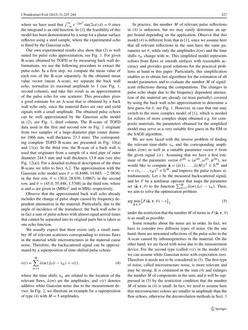
where the time shifts τm are related to the location of therelevant flaws, a(m) are the amplitudes, and ν(t) denotesadditive white Gaussian noise due to the measurement de-vice. In Fig. 2, we illustrate an example for a superpositionof type (4) with M = 5 amplitudes.

In practice, the number M of relevant pulse reflectionsin (4) is unknown, but we may easily determine an up-per bound depending on the application. Observe that thismodel (4) is different from that in [1], since we assume herethat all relevant reflections in the sum have the same pa-rameter set θ , while only the amplitudes a(m) and the timeshifts τm change with m. This simplified model representsechoes from flaws or smooth surfaces with reasonable ac-curacy and provides good solutions for the practical prob-lems at hand in this paper. Particularly, this simplificationenables us to obtain fast algorithms for the estimation of allmodel parameters and to evaluate the number M of signif-icant reflections during the computations. The changes inpulse echo shape due to the frequency dependent attenua-tion of the material are already (at least partially) coveredby using the back wall echo approximation to determine afirst guess for θ , see Fig. 1. However, in case that one mayswitch to the more complex model of [1], which is neededfor echoes of more complex shape obtained e.g. for com-posite materials, the parameters obtained for the simplifiedmodel may serve as a very suitable first guess in the EM orthe SAGE algorithm.

We are now faced with the inverse problem of findingthe relevant time-shifts τm and the corresponding ampli-tudes a(m) as well as a suitable parameter vector θ fromthe given signal s(t). Assuming that we have a first esti-mate of the parameter vector θ(0) = (α(0),ω(0), φ(0)), wewould like to compute a = (a(1), . . . , a(M))T ∈ R

M andτ = (τ1, . . . , τM)T ∈ R

M , and improve the pulse echoes si-multaneously. Let s be the measured backscattered signal,and let F be a nonlinear operator that maps the parameterset (a,τ , θ) to the function

∑Mm=1 a(m)fθ (· − τm). Then,

we aim to solve the optimization problem

arg mina,τ ,θ

∥∥F(a,τ , θ) − s∥∥

2 (5)

under the restriction that the number M of terms in F(a,τ , θ)

is as small as possible.Some remarks about the noise are in order. In fact, we

have to consider two different types of noise. On the onehand, there are unwanted reflections of the pulse echo in theA-scan caused by inhomogeneities in the material. On theother hand, we are faced with noise due to the measurementdevice. For the second type (called ν(t) in the model (4))we can assume white Gaussian noise with expectation zero.Therefore it needs not to be considered in (5). The first typeof noise, called microstructure noise, is more relevant andmay be strong. It is contained in the sum (4) and enlargesthe number M of components in the sum, and it will be sup-pressed in (5) by the restriction condition that the numberM of terms in (4) is small. In fact, we need to assume herethat microstructure echoes are smaller in amplitude than theflaw echoes, otherwise the deconvolution methods in Sect. 3


Fig. 1 Left: vector of mean values from real data (TOFD and back wall detection), middle: separated back wall echo, right: approximation by aGabor function (2), for better comparison the separated back wall echo is presented by a dashed line; time in microseconds


Fig. 2 Example for a pulse echo fθ (t) (left), 5 amplitudes a(m) (middle), and the superposition s(t) = ∑5m=1 a(m)fθ (t − τm)

will not be able to separate them and noise may be wronglytaken as a significant flaw echo, see Sect. 6.

The optimization problem in (5) is very difficult to solvesince the considered operator is nonlinear and not convexwith respect to the parameters. The problem is even moredelicate if the number of significant echoes M is not known.A usual approach to tackle such a complex problem is toseparate it into subproblems that can be solved easier. IfM is known beforehand and small, the EM algorithm (ora generalized version of it) can be employed to compute themaximum likelihood estimation (MLE), [1, 13, 14]. For thatpurpose, the function s(t) = ∑M

m=1 a(m)fθ (t − τm) + ν(t)

is separated into the (unknown) summands

xm = a(m)fθm(t − τm) + νm(t) m = 1, . . . ,M

with∑M

m=1 νm(t) = ν(t). Supposed, that there are given theparameters ak(m), τ k

m, θkm from the kth iteration, one tries

to improve the current expectation of xm in the expectationstep (E-step) by

xkm = ak(m)fθk

m

(· − τ km

) + 1

M

(s −

M∑

m=1

ak(m)fθkm

(· − τ km

))

for m = 1, . . . ,M and solves the minimization problem inthe M-step separately for each m,

(ak+1(m), τ k+1

m , θk+1m

)

= arg mina(m),τm,θm

∥∥xkm − a(m)fθm(· − τm)

∥∥2.

Observe that the M subproblems considered in the EM algo-rithm are only coupled by the condition s ≈ ∑M

m=1 ak(m) ×fθk

m(· − τ k

m) in the expectation step, and this yields the veryslow convergence of the EM algorithm. However, while theconditions that imply convergence to the global minimumof (5) can not be verified (see [13]), the method gives goodparameter estimates, supposed that one starts with a suitablefirst guess.

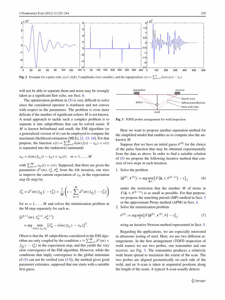
Fig. 3 TOFD probes arrangement for weld inspection

Here we want to propose another separation method forthe simplified model that enables us to compute also the un-known M .

Suppose that we have an initial guess θ(0) for the choiceof the pulse function that may be obtained experimentallyfrom the data as above. In order to find a suitable solutionof (5) we propose the following iterative method that con-sists of two steps in each iteration.

1. Solve the problem(a(k),τ (k)

) := arg mina,τ

∥∥F(a, τ, θ(k−1)

) − s∥∥

2 (6)

under the restriction that the number M of terms inF(a, τ, θ(k−1)) is as small as possible. For that purpose,we propose the matching pursuit (MP) method in Sect. 3or the approximate Prony method (APM) in Sect. 4.

2. Solve the minimization problem

θ(k) := arg minθ

∥∥F(a(k),τ (k), θ

) − s∥∥

2 (7)

using an iterative Newton-method represented in Sect. 5.

Regarding the applications, we are especially interestedin ultrasonic testing of steel. Here, we use two different ar-rangements. In the first arrangement (TOFD inspection ofweld seams) we use two probes, one transmitter and onereceiver, see Fig. 3. The transmitter produces a relativelywide beam spread to maximize the extent of the scan. Thetwo probes are aligned geometrically on each side of theweld, and an A-scan is taken at sequential positions alongthe length of the seam. A typical A-scan usually detects


Fig. 4 Example of TOFDA-scans. Top: A-scan without aflaw; bottom: A-scan with aflaw. These A-scans are takenfrom the TOFD data in Fig. 11

– the lateral signal which travels along the surface of thecomponent and has shortest arrival time;

– the back wall echo, which has longest transit time, seeFig. 4.

In the second arrangement (inspection of back wall defor-mations), transmitter and receiver coincide and the beam isfocussed to the back wall. In case of defects, also the corre-sponding signal reflection can be observed in the A-scan.

Observe that the proposed iteration method that separatesthe optimization of the arrival times and amplitudes fromthe optimization of bandwidth factor, center frequency andphase also gives no guaranty for global convergence. How-ever, using the initial parameter vector θ (0) obtained fromapproximating the back wall echo as given above, we usu-ally obtain reasonable results for the parameters already byusing just the first step of the proposed iteration (and keep-ing the θ = θ (0) just from the approximation).

3 Deconvolution Based on Greedy Algorithms

We are especially interested in fast algorithms for detectionof arrival times in the proposed models. Therefore, we pro-pose first a matching pursuit approach that has been intro-duced in [15], see also [16] and references therein. It hasbeen considered earlier in ultrasonic nondestructive testing;

we refer to [18] as well as to modified versions as high res-olution pursuit [19] and support matching pursuit [20]. Inopposite to [18–20], we apply this idea firstly in connectionwith parameter estimation for the pulse model for blind de-convolution.

Generally, the matching pursuit algorithm works as fol-lows. Let us assume that a given function s in a Hilbertspace H can be well approximated by a linear combinationof given functions bj from a dictionary D = {b1, . . . , bD}.In the first step, one iteratively seeks for the dictionary func-tion bj that correlates best with s. Then the same procedure

is applied to the residuum r1 = s − 〈s,bj 〉‖bj ‖2 bj and so forth. In

order to apply this idea to our model, we first need a suitablediscretization. We suppose in this section that the parametervector θ describing the pulse functions fθ is given, such thatwe have to solve (6) for unknown τ and a and under the re-striction that M is small. A procedure for iterative adjustingof the parameter vector θ will be presented in Sect. 5.

3.1 Discretization of the Model

In practice, the received signal (A-scan) s is given as a vec-tor of sampled signal values s = (s(nΔt ))

Nn=0, where Δt de-

notes the sampling distance and N +1 is the number of data.Further, we can discretize the pulse echo fθ with the

same sampling distance Δt , i.e. let fθ = (fθ (Δt ))L=−L


with 2L N , where we use only a finite number of functionvalues, since fθ decays rapidly. We assume that all relevantshifts of the impulse function fθ (t) are completely recordedby the sampled data. Then a discretization of the receivedsignal s can be modeled by

s(nΔt ) =N−L∑

k=L

a(k)fθ

((n − k)Δt

) + ν(nΔt ),

n = 0, . . . ,N, (8)

where a = (a(k))N−Lk=L denotes the vector of K + 1 (un-

known) amplitudes, where K := N − 2L. A comparisonof this representation of s with the sparse representationin (4) yields that we can suppose that only a small numberM K + 1 of coefficients in a = (a(k))N−L

k=L has a modulusbeing significantly different from zero, and the significantcomponents are assumed to have the indices km ∈ Z withL ≤ k1 < · · · < kM ≤ N −L. Hence, the relevant time-shiftsτm in (4) are given by τm = kmΔt .

We denote the coefficient matrix of the linear systemin (8) by Fθ = Fθ,Δt = (fθ ((n − k)Δt ))

N,N−Ln=0,k=L and can

shortly write

Fθ,Δt a + ν = s, (9)

where ν = (ν(0), ν(Δt ), . . . , ν(NΔt))T is the Gaussian

noise vector modeling the measurement errors while thestructural errors occur as small components in a. Thematrix-vector representation reads⎛

⎜⎜⎜⎜⎜⎜⎜⎜⎜⎜⎜⎜⎜⎜⎜⎜⎜⎝

fθ (−LΔt ) 0 . . . 0

fθ ((−L + 1)Δt ) fθ (−LΔt )...

fθ ((−L + 2)Δt ) fθ ((−L + 1)Δt )

.

.

....

. . . fθ (−LΔt )

fθ (LΔt ) fθ ((−L + 1)Δt )

0 fθ (LΔt )

.

.

.. . .

. . ....

0 . . . 0 fθ (LΔt )

⎞

⎟⎟⎟⎟⎟⎟⎟⎟⎟⎟⎟⎟⎟⎟⎟⎟⎟⎠

a + ν = s.

(10)

This linear system is overdetermined and needs to be solvedapproximately under the restriction that the coefficient vec-tor a is sparse, i.e., contains only M K + 1 elements.Using this discretization, we now look for a solution of theoptimization problem

mina

‖Fθ a − s‖2

under the restriction that the subnorm M = ‖a‖0, i.e. thenumber of nonzero components in a, is small. Here again,the relevant noise is suppressed by this additional restrictionon the size of M and the white noise vector ν with expec-tation zero needs not to be considered in the minimizationproblem.

3.2 Matching Pursuit

Considering the linear system Fθ a + ν = s, we denote thecolumns of the matrix Fθ by f0, . . . , fK , where K = N −2L.Here, {f0, . . . , fK } is the dictionary for our MP method (inthe Hilbert space R

N+1). The system (9) can also be rewrit-ten in the form

s =K∑

k=0

a(k)fk + ν,

(where a(k) := a(k + L)) i.e., s can be approximated by alinear combination of the columns fk . In a first step, we de-termine the index k1 ∈ {0, . . . ,K} such that the column fk1

correlates most strongly with s, i.e.

k1 = arg maxk=0,...,K

∣∣〈s, fk〉∣∣,

where 〈s, fk〉 = sT fk is the standard scalar product of the twovectors s and fk .

In the next step, we determine the coefficient a(k1) suchthat the Euclidean norm ‖s − a(k1) · fk1‖2 is minimal, i.e.a(k1) = 〈s, fk1〉/‖fk1‖2

2, where ‖fk1‖2 denotes the Euclideannorm of fk1 .

Now we consider the residuum r1 = s−a(k1)fk1 and pro-ceed again with the first step, where s is replaced by r1.

Starting with r0 = s and with a = 0, the summarized al-gorithm works in the j -th iteration as follows:

1. Determine an optimal index kj such that fkjcorrelates

most strongly with the residuum rj−1, i.e.

kj = arg maxk=0,...,K

∣∣〈rj−1, fk〉∣∣.

2. Update the coefficient a(kj ) to a(kj )+〈rj−1, fkj〉/‖fkj

‖22,

where 〈rj−1, fkj〉/‖fkj

‖22 solves the problem minx ‖rj−1

− xfkj‖2. Put

rj = rj−1 − a(kj )fkj.

As a stopping criterion, we shall apply the following pro-cedure. We determine a priori an upper bound M for thenumber of coefficients in (4) and a suitable error boundε > 0. Then the MP iteration is stopped after j < M iter-ations if

maxk=0,...,K

∣∣〈rj−1, fk〉∣∣/‖fk‖2

2 < ε,

and at latest after M iterations. Using a sufficiently large up-per bound M for the number of scatterers, the MP iterationwill be stopped by the error bound criterion, and in this waywe can compute the number M of relevant pulse echoes.

Let us shortly consider the numerical complexity of theMP method. For the first step of the algorithm we need


to compute K + 1 = N − 2L + 1 scalar products, wherethe vectors fk have at most 2L + 1 nonzero components.Hence we need (2L + 1)(N − 2L + 1) multiplications,2L(N − 2L + 1) additions as well as the comparisons tofind a maximum of N − 2L + 1 numbers. Here we assumethat L N . For the second step we only need one divisionand one addition to compute a(kj ), where we suppose that‖fk‖2

2 = ∑L=−L fθ (Δt )

2 is preliminarily computed with2L + 1 multiplications and 2L additions. Finally, rj is ob-tained with 2L + 1 multiplications and 2L + 1 additions.Hence the complete MP method with M iterations can beperformed with (4L+ 1)NM −M(4L2 − 2L− 5)+ 4L+ 2arithmetical operations, i.e., it is a O(N) algorithm and istherefore suitable for real time computations.

3.3 Orthogonal Matching Pursuit

The orthogonal matching pursuit algorithm works slightlydifferent, see e.g. [16]. While the first step in each iterationstage is the same as before, the OMP replaces the update ofonly one coefficient a(kj ) by a least square minimization inthe second step, i.e. we use here

2. Update the coefficients a(k1), . . . , a(kj ) such that ‖s −∑j

i=1 a(ki)fki‖2 is minimal and put rj =

s − ∑j

i=1 a(ki)fki.

The least squares minimization problem mina(k1),...,a(kj ) ‖s−∑j

i=1 a(ki)fki‖2 leads to the linear system

(〈fki, fki′ 〉

)j

i,i′=1

(a(ki)

)j

i=1 = (〈s, fki〉)j

i=1. (11)

In case of an orthonormal basis {fk : k = 0, . . . ,K}, the co-efficient matrix is the identity. But in our case, the shifts ofthe pulse function are not orthogonal. However, the num-ber of considered vectors fi is smaller than M and the linearsystem (11) is of small dimension.

The OMP algorithm is more stable than the simple MP al-gorithm, since the update of all amplitudes in each iterationstep ensures a better approximation of the signal s. Pleasenote that this minimization does not effect the vectors fki

themselves that are determined by the columns of Fθ,Δt .However, since we are usually interested in a very smallnumber of significant amplitudes, the MP algorithm alreadyprovides good results while being less time-consuming. Fig-ure 5 in Sect. 6.1 shows the behavior of OMP for a single A-scan. Finally, we remark that the MP and the OMP algorithmof course also work for overlapping echoes, see Sect. 6.1. Inthis case the OMP is more robust.

4 Deconvolution Based on the Approximate PronyMethod

Now, we propose the approximate Prony method (APM),where we can obtain the number M of relevant scatterers

during the algorithm. Furthermore, while the MP algorithmis restricted to a grid for finding the time-shifts τm = kmΔt ,the APM can detect arbitrarily distributed time-shifts. Let usconsider again our sparsity model (4)

s(t) =M∑

m=1

a(m)fθ (t − τm) + ν(t),

where we want to optimize over the time shifts τ =(τ1, . . . , τM), the amplitudes a = (a(1), . . . , a(M)) and thepulse parameters θ , where M is unknown but small. We as-sume here that we have a suitable bound M > M for the truenumber of relevant coefficients and can replace M by M inthe above model. As in the last section, we first assume tohave a good estimate for the parameter vector θ such thatwe can concentrate on the computation of τ and a from thesamples of s. For that purpose, we now adapt the approxi-mate Prony method considered in [17] as follows.

Let the Fourier transform of a function f ∈ L1(R) begiven by

f (ξ) := 1√2π

∫ ∞

−∞f (t)e−iξ t dt.

Applying the Fourier transform to (4) (with M replaced bythe bound M > M), we find

s(ξ ) =(

M∑

m=1

a(m)e−iξτm

)fθ (ξ) + ν(ξ).

In our case, the real-valued Gabor function fθ (t) =Kθe

−αt2cos(ωt + φ) is the real part of gθ (t) = Kθe

−αt2 ×ei(ωt+φ) = Kθe

iφe−αt2eiωt . Hence

fθ (ξ) = 1

2

(gθ (ξ) + gθ (ξ)

)

= Kθ

2√

2α

(eiφe−(ω−ξ)2/4α + e−iφe−(ω+ξ)2/4α

). (12)

Particularly, the function fθ (ξ) possesses only a zero at ξ =0 if φ = (2π+1)π

2 while f (ξ) = 0 for all ξ = 0. Avoiding thecase ξ = 0, we can hence write

h(ξ) := s(ξ )

fθ (ξ)=

M∑

m=1

a(m)e−iξτm + ε(ξ ),

where the noise term ε(ξ ) := ν(ξ)/fθ (ξ) is assumed to besmall.

For given samples h(kΔξ ), (where Δξ is a fixed samplingdistance) we now aim to compute the frequencies τm ∈ R+and the corresponding amplitudes a(m), for m = 1, . . . , M

separately using the following method. We consider the


polynomial

Λ(z) =M∏

m=1

(z− e−iΔξ τm

) = λM

zM +λM−1z

M−1 +· · ·+λ0

with λM

= 1 that possesses the exponentials e−iΔξ τm withthe unknown time-shifts τm as zeros.

In a first step, we will determine the coefficients λk of thepolynomial Λ(z). We observe that for given sample valuesh((k + )Δξ ), k = 0,1, . . . , and = 1,2, . . . , we have

M∑

k=0

λkh((k + )Δξ

)

=M∑

k=0

λk

M∑

m=1

a(m)e−iτmΔξ (k+) +M∑

k=0

λkε((k + )Δξ

)

≈M∑

m=1

a(m)e−iτmΔξ

M∑

k=0

λk

(e−iτmΔξ

)k

= Λ(e−iτmΔξ

) M∑

m=1

a(m)e−iτmΔξ = 0,

where we have assumed that the noise term∑M

k=0 λkε((k +)Δξ ) is negligibly small.

Using the above relation for = 1,2, . . . , M + 1, the un-known coefficients λ0, . . . , λM−1 of Λ(z) can be computedby finding an approximate zero eigenvector of the Hankelmatrix

H =

⎛

⎜⎜⎝

h(Δξ ) h(2Δξ) . . . h((M + 1)Δξ )

h(2Δξ) h(3Δξ) h((M + 2)Δξ )

.

.

....

h((M + 1)Δξ ) h((M + 2)Δξ ) . . . h((2M + 1)Δξ )

⎞

⎟⎟⎠ .

We can now obtain the true number M < M of suitableterms in the model (4) by a rank estimation of H, sincethe rank of the matrix H in the noiseless case coincideswith the number M of suitable terms, see [17]. We applythe above eigenvalue problem to a Hankel matrix H of size(M + 1) × (M + 1), i.e., we compute an approximate zeroeigenvector of H. This eigenvector contains the coefficientsλk that are used to form the polynomial Λ(z). We evaluatethe corresponding zeros of the polynomial Λ(z). The zerosof Λ that are relevant to us, are of the form e−iτmΔξ andlie (approximately) on the unit circle, such that we are ableto determine the time shifts τm, m = 1, . . . ,M . As shownin [17], each zero eigenvector of H will yield the same rele-vant zeros e−iτmΔξ .

In the second part of the procedure, we can compute theamplitudes am as least square solution of the overdetermined

linear system

M∑

m=1

amfθ (Δt − τm) = s(Δt ), = 0, . . . ,N,

thereby neglecting the noise function ν(t).For application of the first step of above procedure, we

need to evaluate the Fourier transform h = s/fθ at suitablevalues kΔξ . For this purpose we employ the fast Fouriertransform as follows. Assume that we have given the sam-pled values of the backscattered signal s = (s(Δt ))

N=0. Us-

ing linear splines, s can be approximated by the sum

s(t) =N∑

=0

s(Δt )N2(t − Δt ),

where the B-spline N2 has the support [−(Δt )−1, (Δt )

−1]and is given by N2(t) = (1 − Δt |t |) for t ∈ [−(Δt )

−1,

(Δt )−1]. Then Fourier transform yields

ˆs(ξ) =(

N∑

=0

s(Δt )e−iξΔt

)N2(ξ).

With N2(ξ) = 1√2π

1Δt

sinc( ξ2Δt

)2 and with the function

fθ (ξ) that is explicitly given in (12), we obtain the approxi-mate values

h

(2πkΔt

)= h(kΔξ ) = ˆs(kΔξ )

f (kΔξ ),

where Δξ := 2πΔt

, k = 0, . . . ,N , and where

N∑

=0

s(Δt )e−iξkΔt , k = 0, . . . ,N

is computed for ξk = 2πkΔt

by the fast Fourier transform.

Remark 1 Compared with the MP method, the APM hasthe advantage that we are able to compute the time shiftsτm exactly independently from the sampling grid with sam-pling size Δt . However, due to the needed Fourier trans-form, APM is computationally more expensive than the MPmethod. Although APM has been established for noisy datameasurements in [17], it is more sensitive to noise than theMP method.

Remark 2 The APM method is able to find relevant time-shifts τm with a small separation distance, i.e. it works alsofor overlapping pulse echoes, see Sect. 6.1. The separationdistance influences the numerical stability of the algorithm.It can be chosen smaller if the number of data N is large(see [17]).


Remark 3 The MP (OMP) method and the APM methodare fundamentally different with respect to their underlyingideas as well as to their numerical effort. The MP method isa greedy method, i.e. it will find the most significant am-plitudes just by comparison of correlations of the shiftedpulse echo with the measured data. While this method isvery simple and efficient, it can fail for all further iterationsif once a wrong shift is taken (possibly caused by strongnoise). The number M of relevant scatters is found by us-ing an initial bound for M and by observing the size of theremainder if the detected significant pulse echoes are sub-tracted from the data. The APM method is much smarter. Itseparates the search of arrival times from the determinationof the corresponding amplitudes by transferring the modelto the frequency domain. Unfortunately, the Fourier trans-form can enforce the errors such that this method is moresensitive to low SNR values.

5 Optimization of the Parameters

In the preceding sections we have assumed that a reliableestimate of the parameter vector θ determining the pulseecho is given. In Sect. 2, we have proposed an alternatingminimization procedure for the stepwise improvement of thepulse echo parameters during the computation process.

Having solved the optimization problem (6) for small M

using either the matching pursuit algorithm or the approxi-mate Prony method, we shall now consider the second min-imization problem (7) for adjusting the parameter vector θ .For that purpose we want to employ the iterative Newtonmethod. Consider now the minimization problem

θ(k) := arg minθ

∥∥F(a(k),τ (k), θ

) − s∥∥

2.

A linearization of the operator around an initial guess θ(k−1)

yields

F(a(k),τ (k), θ (k−1) + dθ

)

≈ DθF(a(k),τ (k), θ (k−1)

)dθ + F

(a(k),τ (k), θ (k−1)

).

Here, DθF(a(k),τ (k), θ (k−1)) denotes the Jacobian of F atθ(k−1), i.e.,

DθF(a(k),τ (k), θ (k−1)

)

=(

∂F (a(k),τ (k), θ (k−1))

∂α,∂F (a(k),τ (k), θ (k−1))

∂ω,

∂F (a(k),τ (k), θ (k−1))

∂φ

).

Hence, the update vector dθ = (dα, dω,dφ)T is obtainedfrom the equation

DθF(a(k),τ (k), θ (k−1)

)dθ + F

(a(k),τ (k), θ (k−1)

) = s

and can be evaluated at the known samples kΔt . This leadsto a least squares problem which can be solved directlysince the corresponding coefficient matrix has only three di-mensions. In this way, we obtain the new update θ

(k−1)1 :=

θ(k−1) + dθ . One may proceed with the Newton iteration toobtain the updates θ

(k−1)2 , θ

(k−1)3 , . . . . After r Newton steps,

where r that can be just fixed or can depend on some suitableerror criterion, one obtains the new estimate θ(k) = θ

(k−1)r .

Unfortunately, because of the complicated normalizationfactor Kθ in (3), the vector DθF(a(k),τ (k), θ (k−1)) can noteasily be computed analytically. Therefore, we consider ananalytical representation of

Dθ

(1

Kθ

F(a,τ , θ)

)

= Dθ

(M∑

m=1

a(m)e−α(t−τm)2cos

(ω(t − τm) + φ

))

and obtain for θ = (α,ω,φ)T ,

Dθ

(1

Kθ

F(a,τ , θ)

)

=

⎛

⎜⎜⎜⎜⎜⎜⎝

−M∑

m=1a(m)(t − τm)2e−α(t−τm)2

cos(ω(t − τm) + φ)

−M∑

m=1a(m)(t − τm)e−α(t−τm)2

sin(ω(t − τm) + φ)

−M∑

m=1a(m)e−α(t−τm)2


⎞

⎟⎟⎟⎟⎟⎟⎠

T

.

However, a change of the parameter vector θ implies a possi-bly considerable change of the norm K−1

θ of the pulse func-tion fθ . Disregarding the normalization factor Kθ thus leadsto a highly unstable method since the amplitudes in a areoptimized with respect to the Euclidean norm of fθ . In or-der to counter this problem we are updating not only θ ineach Newton step but also the amplitudes a. In this way theamplitudes in a are adjusted to the changing wave norm.Therefore, we employ

Dθ,a

(1

Kθ

F(a,τ , θ)

)

=

⎛

⎜⎜⎜⎜⎜⎜⎜⎜⎜⎜⎜⎜⎜⎝

−M∑

m=1a(m)(t − τm)2e−α(t−τm)2

cos(ω(t − τm) + φ)

−M∑

m=1a(m)(t − τm)e−α(t−τm)2


−M∑

m=1a(m)e−α(t−τm)2


e−α(t−τ1)2cos(ω(t − τ1) + φ)

...

e−α(t−τM)2cos(ω(t − τM) + φ)

⎞

⎟⎟⎟⎟⎟⎟⎟⎟⎟⎟⎟⎟⎟⎠

T

in the iterative Newton method and update not only the pa-rameter vector θ but also the coefficient vector a in our


model (4). Our numerical results in Sect. 6.3 show the fastconvergence of the iterative Newton method after only a fewiteration steps.

For the numerical application of this procedure for pa-rameter optimization we refer to Sect. 6.3.

6 Test Results

We have tested the proposed procedures using simulateddata as well as real data, particularly TOFD data of welddefects and TOA data of back wall deformations.

6.1 Simulated Data

In a first test, we want to show the performance of the OMP-method and the APM method to recover arrival times andamplitudes of a sum of four interfering echoes with differentSNR. For that purpose, we consider two different scenarios.In the first scenario we have four interfering echoes beingobtained by four shifts of the Gabor function fθ with pa-rameters α = 50(MHz)2, ω = 25.1327 MHz and φ = 0.52microseconds. The resolution is 10 ns. Particularly, we studythe behavior of the two deconvolution methods if one ar-rival time comes close to another in case of almost no noise(SNR of about 45.00). The four overlapping echoes con-sidered in Table 1 are illustrated in Fig. 5, top. In particu-lar, one can observe that if the arrival time x of the thirdecho is approaching the fourth echo at arrival time 7.20 with7.15 ≤ x < 7.20 it is really difficult to recognize x and 7.20as two different arrival times. For APM, the computed ar-rival times are rounded corresponding to the resolution. Theobtained results, summarized in Table 1, show that the twoproposed algorithms are suited also for recovering interfer-ing echoes. In this (almost noiseless) case the APM is morestable than OMP when the arrival times of two echoes ap-proach. If the echoes are too close, then OMP can not longerdistinguish between them and takes it as one echo, wherethe amplitudes are added. For approaching arrival times with7.15 ≤ x < 7.20, the OMP finds only one arrival time whilethe APM method recognizes two arrival times, where for adifference of 0.01 microseconds the corresponding ampli-tudes are not longer correctly attributed.

In the second scenario, we consider four shifts of theGabor function fθ with parameters α = 20(MHz)2, ω =50.2634 MHz and φ = 0.52 microseconds. We study the be-havior of the deconvolution methods for changing low SNR,see Table 2. The corresponding noisy echo functions are il-lustrated in Fig. 5, bottom. In particular, we observe that thetwo algorithms correctly estimate the four arrival times evenin case of strong noise, while the obtained amplitudes are notexact. We remark that the MP algorithm works only slightlyworse than OMP in the two experiments and is in fact asgood as OMP for high noise levels.

Considering the data, there are mainly two componentsof noise: (a) microstructure noise, produced by multiple re-flections and inhomogeneous material, and (b) electronicnoise, fed from cables, amplifiers etc., which act like a band-pass filter. The first can be considered as Gaussian noise inthe coefficient vector a, which results in colored noise af-ter convolution with the wave. Hence, to test the algorithmswith different noise levels and different wave forms we havemodeled a back wall deformation as follows.

We have used the data in Fig. 6 that originates fromthe measurement of a real back wall deformation in asteel pipe that has been extended by zero outside its sup-port. Then, Gaussian noise with different variances (0.001,0.01 and 0.025) has been added to the back wall data be-fore convolving each column with a Gabor function of theform (2). We want to illustrate that the proposed deconvo-lution methods perform well for different Gabor functions.The simulated B-scans in the first row of Fig. 8 are ob-tained using the convolution with the Gabor function withθ = (α,ω,φ) = (20,10,0), where the bandwidth factor α

is given in (MHz)2, and the center frequency ω in MHz.Analogously, the B-scans in the first row of Fig. 9 are ob-tained by convolution of the noisy geometric model with aGabor function with θ = (7.5,10,π/2). The two differentGabor functions are illustrated in Fig. 7. Observe that herenoise simulates microstructure noise produced by inhomo-geneities in the material since the noise has been added be-fore the convolution with the pulse function.

In the second and third rows of Figs. 8 and 9, we illus-trate the behavior of the proposed MP resp. OMP algorithm.The reconstructed back wall echo time yields the wall thick-ness of the modeled tube correctly up to the discretizationerror. In the second row of Fig. 8, we present the ampli-tudes of significant reflections of the pulse function com-puted with the matching pursuit (MP) method. In this casea nearly nonnegative Gabor wave is used as pulse function.The MP method has been used with at most M = 5 itera-tions and with ε = 1.0 in the first, ε = 1.75 in the second,and ε = 1.5 in the third column. Applying again a convo-lution to the obtained sparse A-scan vectors, we find a suit-able approximation of the original B-scan (see third row inFig. 8). This sparse approximation efficiently denoises theoriginal B-scan. The same experiment is performed with theAPM proposed in Sect. 4. The fourth row of Fig. 8 illustratesthe amplitudes of significant reflections of the pulse func-tion computed with the approximate Prony method. Here thenumber of significant amplitudes is found during the algo-rithm and it swings between 1 and 8 with an average of 1.65.Applying a convolution to the sparse A-scans we obtain theapproximation presented in the last row of Fig. 8.

Figure 9 shows the denoising results taking an antisym-metric Gabor wave as pulse echo and using OMP and APM.The OMP method is used here with M = 5 and with ε =


Fig

.5To

p:Fo

urin

terf

erin

gec

hoes

ofth

eG

abor

func

tion

fθ

with

θ=

(50(

MH

z)2,25

.132

7M

Hz,

0.52

µs)

(alm

ostn

oise

less

case

)with

ampl

itude

san

dar

riva

ltim

esas

give

nin

Tabl

e1

forx

=6.

96(l

eft)

,x=

7.07

(mid

dle)

and

x=

7.15

(rig

ht);

Bot

tom

:Fou

rin

terf

erin

gec

hoes

ofth

eG

abor

func

tion

fθ

with

θ=

(20(

MH

z)2,50

.263

4M

Hz,

0.52

µs)

with

ampl

itude

san

dar

riva

ltim

esas

give

nin

Tabl

e2,

with

outn

oise

(lef

t),w

ithSN

Rof

19.3

4(m

iddl

e)an

dw

ithSN

Rof

4.75

(rig

ht);

time

inm

icro

seco

nds


Table 1 Parameter estimation results for four interfering echoes when one arrival time gets close to another. The SNR of the interfering echoes isabout 45

Actualparameters

Arrival times (µs) Amplitudes

0.50 3.40 x 7.20 3.0 −2.0 2.5 4.0

time x Arrival times (µs) obtained by OMP Amplitudes obtained by OMP

6.96 0.50 3.40 6.96 7.20 3.0028 −1.9937 2.5001 3.9988

7.07 0.50 3.40 6.95 7.21 3.0023 −2.0012 −1.3483 2.4355

7.15 0.50 3.40 7.18 2.9950 −1.9958 5.1517

7.18 0.50 3.40 7.19 3.0030 −1.9950 6.2750

7.19 0.50 3.40 7.20 2.9996 −2.0000 6.3707

time x Arrival times (µs) obtained by APM Amplitudes obtained by APM

6.96 0.50 3.40 6.96 7.20 2.9998 −1.9955 2.5013 3.9999

7.07 0.50 3.40 7.07 7.20 3.0007 −2.0023 2.5008 4.0031

7.15 0.50 3.40 7.15 7.20 3.0048 −1.9918 2.5027 4.0220

7.18 0.50 3.40 7.18 7.20 3.0014 −1.9979 2.1900 4.3127

7.19 0.50 3.40 7.20 7.21 3.0006 −1.9994 6.0532 0.4065

Table 2 Parameter estimation results for four interfering echoes with different SNR. For OMP the parameter ε = 1.25 is taken and the upperbound for arrival times is 5

Actualparameters

Arrival times (µs) Amplitudes

0.50 3.40 3.75 7.20 3.0 −2.0 4.0 2.5

SNR Arrival times (µs) obtained by OMP Amplitudes obtained by OMP estimationSNR

19.34 0.50 3.40 3.75 7.20 3.1000 −1.9727 3.9863 2.4562 34.22

13.10 0.50 3.40 3.75 7.20 3.1071 −1.9352 3.9093 2.4312 30.88

8.15 0.50 3.40 3.75 7.20 3.1085 −1.7118 3.9806 2.4363 25.37

4.75 0.50 3.40 3.75 7.19 4.0206 −2.5048 3.4768 1.9641 10.33

SNR Arrival times (µs) obtained by APM Amplitudes obtained by APM estimationSNR

19.34 0.50 3.40 3.75 7.20 3.1107 −2.0841 3.9907 2.5646 28.85

13.10 0.50 3.40 3.75 7.20 3.0815 −2.0384 3.9552 2.5659 20.34

8.15 0.50 3.40 3.75 7.20 2.9960 −2.4391 4.3420 2.4048 18.13

4.75 0.50 3.39 3.75 7.20 3.7694 −2.8166 3.2185 2.2643 10.30

1.0;1.25;1.5 in the rows 1, 2, 3. The advantage of the APMis the ability to detect the significant translations without anunderlying grid. In order to present these data in the fig-ures (fourth row in Figs. 8 and 9), we have considered a tra-verse through the obtained amplitudes (approximation witha linear B-spline) instead of rounding the found significanttranslations to the grid points. Therefore the obtained sig-nificant amplitudes are slightly different for the MP methodand APM.

Besides the correct estimation of the arrival times foundby the two deconvolution algorithms in the above experi-ment, we obtain a sparse approximation of the B-scans interms of a small number of significant coefficients repre-senting the relevant information. The number of significantcoefficients found by MP/OMP resp. APM is presented in

Table 3. Figs. 8 and 9 show that it is possible to reconstructthe B-scan using only these significant coefficients. Observ-ing that the B-scans in Figs. 8 and 9 have 115 columns and279 resp. 298 rows, we obtain compression rates as given inTable 3.

We observe, that the MP and the OMP give reasonable re-sults even for highly noisy data. The APM works accuratelyfor the low-level noise case. The reason for that behavior is,that MP/OMP are rather robust algorithms whereas the APMis slightly less numerically stable for high noise levels. Thusthe MP/OMP methods are more suitable for a fast determi-nation of material defects while the APM is able to identifyclustered defects in the low-level noise case, and may beespecially appropriate for determining the more exact struc-


ture of a defect, after knowing where that defect is located.This problem will be considered further in the future.

6.2 Real Data

We study the results of the deconvolution methods for realTOFD data and for back wall echoes.

The original TOFD data in Fig. 10(a), and in Fig. 11(a)has been obtained from a sample of a large-diameter pipe

Fig. 6 3D illustration of the back wall deformation used in the simu-lations

(outer diameter 1066 mm, wall thickness 23.3 mm). InFig. 10(a), the weld seam has been tested with a TOFDsystem (Olympus Omniscan iX) with a 5 MHz transducer,6 mm diameter (Olympus C543-SM). In Fig. 11(a), a10 MHz transducer, 6 mm diameter (Olympus C563-SM)with the same system has been used. Both transducers wereapplied with a wedge with 70° angle of incidence. The flawsin Fig. 10(a) are pores, while Fig. 11(a) shows a lack of fu-sion at the end of the pipe, where the last part of the weldseam has been ground. Both B-scans are measured with asampling rate of 100 MHz and an 8-bit resolution. The res-olution in scan direction is 0.5 mm.

For TOFD signals the lateral signal as well as the backwall echo have generally significantly larger amplitudes thanthe signals indicating defects. In order to obtain the essen-tial signals indicating weld deformations, we add suitableweights that can be chosen a priori using knowledge aboutthe thickness of the tube and an estimate about positions oflateral signal and back wall echo in the A-scan. Since theultrasonic wave send out by the emitter is not given, we esti-mate it from the given data in order to find a first approxima-tion of the pulse echo of the form (2). This is done as givenin Sect. 2, see Fig. 1.

In Figs. 10(b) and 11(b), the results of the MP method(in Sect. 3.2) are shown. We obtain only very few nonzerovalues for each A-scan vector a. Here in each column, wehave taken in the first example (Fig. 10(b)) at most M = 10

Table 3 Comparison of the found mean number M of significant coefficients in each row for different noise levels, and the correspondingcompression rates, see also Figs. 8 and 9

Figure Noisevariance

SNR MP/OMP APM

mean M compression rate mean M compression rate

Figure 8 0.001 16.30 1.2000 0.0043 1.6348 0.0059

0.010 6.50 1.0087 0.0036 1.4609 0.0052

0.025 2.52 1.8696 0.0067 2.0087 0.0072

Figure 9 0.001 18.25 1.3304 0.0045 1.6696 0.0056

0.010 8.42 1.3130 0.0044 1.2348 0.0041

0.025 4.38 1.5130 0.0052 1.8783 0.0063

Fig. 7 Gabor pulse functionsused for simulations of B-scansin Figs. 8 and 9. Left: evenGabor function, right: oddGabor function


Fig. 8 Top: simulated back wallecho with different noise levelsand nearly nonnegative Gaborwave, noise levels from left toright (Gaussian variance):0.001, 0.01, 0.025; second row:obtained significant amplitudesafter deconvolution with MP;third row: back wallreconstruction using only thesignificant amplitudes found byMP; fourth row: obtainedsignificant amplitudes usingAPM; last row: back wallreconstruction using only thesignificant amplitudes found byAPM

nonzero values, where M is the upper bound for the num-ber of iterations of MP, and we have used the error boundε = 40. For the example in Fig. 11(b), (M, ε) = (6,60) hasbeen taken. For a better illustration, Figs. 10(c) and 11(c)show again the positions the nonzero coefficients, where“black” stands for nonzero and “white” for zero coefficients.Finally, the Figs. 10(d) and 11(d) show an approximationof the TOFD data, where only the nonzero coefficients ob-tained by MP, are again convolved with the pulse function.Hence, these representations can be seen as sparse approx-imations of the TOFD B-scans, and also yield a denoised

image. However, most important for further investigation ofpossible flaws are the geometric data in (b) resp. (c).

In a third example we test the MP method for a backwall measurement. The B-scan of the back wall with scrapmark (Fig. 12(a)) originates from a sample of a steel pipeof outer diameter 244.5 mm and wall thickness 13.8 mm. Ithas also been measured with the Omniscan iX system wherewe used a 4 MHz broadband transducer of 15 mm diameter(Karl Deutsch STS 15 WB 2-7) with nominal incidence an-gle. The resolution in scan direction is 0.5 mm and the sam-pling rate is 100 MHz with an 8-bit resolution. As before, weapply the MP method to each A-scan (each column) with


Fig. 9 Top: modeled back wallecho with different noise levelsand antisymmetric Gabor wave,noise levels from left to right(Gaussian variance): 0.001,0.01, 0.025; second row:obtained significant amplitudesafter deconvolution with OMP;third row: back wallreconstruction using only thesignificant amplitudes found byOMP; fourth row: obtainedsignificant amplitudes usingAPM; last row: back wallreconstruction using only thesignificant amplitudes found byAPM

at most M = 5 iterations and with ε = 15, where the MPprocedure is stopped if the error does not exceed ε and (atlatest) after M iterations. Figure 12(b) shows the nonzerocoefficients of the a vectors in each column. For a betterillustration, the nonzero coefficients are black and the zerocoefficients are white in Fig. 12(c). Finally, Fig. 12(d) showsthe result of a convolution of the sparse matrix in (b) withthe pulse yielding a sparse approximation (and a denoising)of the original data. At last, we remark that the used MPand OMP methods are suitable for real time computations.For the complete computation of all arrival times and ampli-tudes for data in Figs. 10–12 together with the computation

of the approximation of s in (d), our MATLAB MP algo-rithm using a 2.66 GHz Intel Core 2 Duo processor needsless than 0.1 seconds while the OMP requires 1 second forthe data Fig. 10 (data size 356×441), 0.9 seconds for Fig. 11(data size 356×331), and 0.65 seconds for Fig. 12 (data size636 × 201).

6.3 Simulations for Parameter Optimization

Finally, we want to illustrate the power of the proposed it-erative Newton method for estimation of parameters in thepulse function model. For this purpose, we have used the


Fig. 10 (a) Original TOFD data; (b) approximative solution of a withMP method in Sect. 3.2; (c) nonzero elements of the solution; (d) ap-proximation of s ≈ F · a

Fig. 11 (a) Original TOFD data; (b) approximative solution of a withMP method in Sect. 3.2; (c) nonzero elements of the solution; (d) ap-proximation of s ≈ F · a

following simulation. In a first step we have randomly cho-sen four amplitudes of different sizes in a vector of length100. Further we have added some Gaussian noise to the vec-tor (simulating microstructure noise) and have convolved theobtained vector with a Gabor function of type (2). The ob-tained A-scan simulation has been now processed as fol-lows. We have taken an initial guess of a Gabor functionwith parameter vector θ0, and have applied the alternatingalgorithm (MP algorithm and iterative Newton method) asproposed in Sect. 2.

Fig. 12 (a) Original B-scan of a backwall; (b) approximative solutionof a with MP method; (c) nonzero elements of the solution; (d) approx-imation of s ≈ F · a

In our first example without noise, we started with θ0 =(35,19,1.54) (α in (MHz)2 and ω in MHz) quite far awayfrom the true parameter vector. The true parameters havebeen obtained already after 6 iterations of the method,namely θ = (5.0,9.0,π/2), see Fig. 13. Since there is nonoise, we obtain a perfect approximation of the A-scan andtherefore omitted the corresponding illustration.

In the second and third example, Gaussian noise of vari-ance 0.01 has been used before convolving the vector withthe Gabor function, this corresponds to the SNR 23.7. InFig. 14, the starting parameter vector is θ0 = (12.5,7.0,1.2).Again we obtain a good estimate of the correct parametervector θ = (5.0,9.0,π/2) already after 6 iterations. The il-lustrations in the first row of Fig. 14 show the parametersα,ω and φ after each iteration, the second row shows the ap-proximation of the true Gabor function with the help of thefound parameter vector and the approximation of the A-scanusing 4 amplitudes found by the MP algorithm. Finally, inthe last example in Fig. 15 a symmetric Gabor function hasbeen used with θ = (5.0,9.0,0), while the starting vectorhas been taken θ0 = (11.5,7.7,0.17). Again, the procedureapproximately finds the correct parameters.

7 Conclusions and Outlook

The deconvolution methods presented in this work are sup-posed to be used as a preprocessing step for further applica-tions. Our long term objective is to derive a method to invertthe B-scans, see [21]. We would like to reconstruct the shapeof the back wall based on the B-scan image. Usually, suchinversion techniques provide better results if the raw data


Fig. 13 Wave parameters (y-axis) against iteration steps (x-axis) (left α, middle ω, right φ) a not noisy

Fig. 14 Top: wave parameters after each iteration step (left α, middle ω, right φ); bottom: original (blue) and approximated (red) wave (left) anddata (right); added Gaussian noise of variance 0.01 to a

only contains low-level noise, and they tend to be unstableif the raw data is too noisy. Hence, it is important to apply afast and effective denoising algorithm that is capable to pre-serve the important signal features while removing most ofthe noise.

In this paper, we have proposed two different deconvolu-tion algorithms that both map an A-scan to a sparse vectorthat still contains the relevant information of the A-scan inan encoded form. This sparse representation of the A-scanresp. the B-scan can be differently processed:

Flaw detection A comparison of the significant coeffi-cients in the sparse columns of the B-scan (after deconvo-lution) provides the positions of significant flaws in the ma-terial. Respectively, in the case of weld seam inspection, thesparse B-scan can be processed further by a direct inver-sion method, see [21]. Alternatively, a representation of theB-scan with only a few coefficients can be used for classi-fication using machine-learning algorithms. The algorithm“learns” the B-scans corresponding to different classes (e.g.for different flaws in the back wall) and afterwards tries to


Fig. 15 Top: wave parameters after each iteration step (left α, middle ω, right φ); bottom: original (blue) and approximated (red) wave (left) anddata (right), added Gaussian noise of variance 0.01 to a

assign the correct class to a new unknown B-scan. In suchlearning procedures, the algorithms are usually not able tohandle full images but only a very limited number of rep-resenting attributes. Therefore, the nonzero coefficients pro-vided by our deconvolution algorithms will act as a goodchoice of representing attributes for such machine learningalgorithms.

Denoising A convolution of the obtained sparse vectorswith the (computed or estimated) pulse echo yields a de-noised B-scan. Since the deconvolution algorithms are suit-ably adapted to the measured signals (by using the trans-mitted pulse echo), this denoising method outperforms mostdirect (non-adaptive) denoising methods for images (see e.g.Figs. 10–12).

Compression Another advantage of our proposed algo-rithm is that the nonzero coefficients provide a strong com-pression of the B-scan. The whole B-scan is reduced to asmall number of most significant coefficients, representingthe relevant information. Knowing the shape of the pulse, itis possible to reconstruct the B-scan only with the knowl-edge of the position of the sparse nonzero coefficients. Ap-

parently, this can be used to reduce the amount of storagesignificantly.

Acknowledgements We thank the referees and the editor for theirvaluable suggestions that led to a considerable improvement of themanuscript. This work is supported by the Central Innovation Pro-gramme SME (ZIM) of the Federal Ministry of Economics and Tech-nology (BMWi) of Germany. We also would like to thank Vallourec &Mannesmann Deutschland GmbH for their financial support.

Open Access This article is distributed under the terms of the Cre-ative Commons Attribution License which permits any use, distribu-tion, and reproduction in any medium, provided the original author(s)and the source are credited.

References

1. Demirli, S., Saniie, J.: Model-based estimation of ultrasonicechoes. Part I: analysis and algorithms. IEEE Trans. Ultrason. Fer-roelectr. Freq. Control 48(3), 787–802 (2001)

2. Kaaresen, K.F., Bolviken, E.: Blind deconvolution of ultrasonictraces accounting for pulse variance. IEEE Trans. Ultrason. Ferro-electr. Freq. Control 46(3), 564–573 (1999)

3. Mendel, J.M.: Optimal Seismic Deconvolution: An Estimation-Based Approach. Academic Press, New York (1983)

4. Walden, A.T.: Non-Gaussian reflectivity, entropy, and deconvolu-tion. Geophysics 50(12), 2862–2888 (1985)


5. Ciang, H.-H., Nikias, C.L.: Adaptive deconvolution and identifi-cation of nonminimum phase FIR systems based on cumulants.IEEE Trans. Autom. Control 35(1), 36–47 (1990)

6. Nandi, A.K., Mämpel, D., Roscher, B.: Comparative study of de-convolution algorithms with applications in non-destructive test-ing. IEE Dig. 145, 1/1–1/6 (1995)

7. Neelamani, R., Choi, H., Baraniuk, R.: ForWaRD: Fourier-wavelet regularized deconvolution for ill-conditioned systems.IEEE Trans. Ultrason. Ferroelectr. Freq. Control 52(2), 418–432(2004)

8. Herrera, R.H., Orozco, R., Rodriguez, M.: Wavelet-based decon-volution of ultrasonic signals in nondestructive evaluation. J. Zhe-jiang Univ. Sci. 7(10), 1748–1756 (2006)

9. Olofsson, T.: Computationally efficient sparse deconvolution of B-scan images. In: Proc. IEEE Ultrason. Symp., pp. 540–543 (2005)

10. Olofsson, T., Wennerström, E.: Sparse deconvolution of B-Scanimages. IEEE Trans. Ultrason. Ferroelectr. Freq. Control 54(8),1634–1641 (2007)

11. Demirli, S., Saniie, J.: Model-based estimation of ultrasonicechoes. Part II: nondestructive evaluation applications. IEEETrans. Ultrason. Ferroelectr. Freq. Control 48(3), 803–811 (2001)

12. Ziskind, I., Wax, M.: Maximum likelihood localization of multi-ple sources by alternating projection. IEEE Trans. Acoust. SpeechSignal Process. 36(10), 1553–1560 (1988)

13. Wu, C.F.J.: On the convergence properties of the EM algorithm.Ann. Stat. 11(1), 95–103 (1983)

14. Chung, P.J., Böhme, J.F.: Comparative convergence analysis ofEM and SAGE algorithms in DOA estimation. IEEE Trans. SignalProcess. 49(12), 2940–2949 (2001)

15. Mallat, S., Zhang, Z.: Matching pursuits with time-frequency dic-tionaries. IEEE Trans. Signal Process. 41, 3397–3415 (1993)

16. Tropp, J.: Greed is good: algorithmic results for sparse approxi-mation. IEEE Trans. Inf. Theory 50, 2231–2242 (2004)

17. Peter, T., Potts, D., Tasche, M.: Nonlinear approximation by sumsof exponentials and translates. SIAM J. Sci. Comput. 33(4), 1920–1944 (2011)

18. Ruiz-Reyes, N., Vera-Candeas, P., Curpián-Alonso, J., Mata-Campos, R., Cuevas-Martinez, J.C.: New matching pursuit-basedalgorithm for SNR improvement in ultrasonic NDT. NDT E Int.38, 453–458 (2005)

19. Ruiz-Reyes, N., Vera-Candeas, P., Curpián-Alonso, J., Cuevas-Martinez, J.C., Blanco-Claraco, J.L.: High-resolution pursuit fordetecting flaw echoes close to the material surface in ultrasonicNDT. NDT E Int. 39, 487–492 (2006)

20. Mor, E., Azoulay, A., Mayer, A.: A matching pursuit method forapproximate overlapping ultrasonic echoes. IEEE Trans. Ultrason.Ferroelectr. Freq. Control 57(7), 1996–2004 (2010)

21. Boßmann, F.: Entwicklung einer automatisierten Auswertung vonbildgebenden Ultraschallverfahren. Diploma thesis, University ofDuisburg-Essen, Germany (2009)

application on tofd and wall thickness measurements · j nondestruct eval (2012) 31:225–244 doi...

Documents