application programming: data mining and data warehousing ... · pdf filedata mining and data...

Projekt współfinansowany ze środków Unii Europejskiej w ramach Europejskiego Funduszu Społecznego

ROZWÓJ POTENCJAŁU I OFERTY DYDAKTYCZNEJ POLITECHNIKI WROCŁAWSKIEJ

Wrocław University of Technology

Internet Engineering

Henryk Maciejewski

APPLICATION PROGRAMMING:

DATA MINING

AND DATA WAREHOUSING

PRACTICAL GUIDE Data Mining and Data Warehousing

Wrocław 2011

Wrocław University of Technology

Internet Engineering

Henryk Maciejewski

APPLICATION PROGRAMMING:

DATA MINING AND DATA WAREHOUSING

PRACTICAL GUIDE Data Mining and Data Warehousing

Wrocław 2011

Copyright © by Wrocław University of Technology

Wrocław 2011

Reviewer: Olgierd Unold

ISBN 978-83-62098-24-8

Published by PRINTPAP Łódź, www.printpap.pl

Contents

Introduction ............................................................................................................................................. 4

PART I Data Mining .................................................................................................................................. 5

Formulation of the Problem Solved in this Guide ............................................................................... 5

Building a Predictive Model in Enterprise Miner ................................................................................ 7

Preparatory tasks ............................................................................................................................ 8

Sample data ..................................................................................................................................... 9

Explore data ................................................................................................................................... 12

Modify data ................................................................................................................................... 17

Build predictive models ................................................................................................................. 22

Assessment of performance of the models .................................................................................. 30

Scoring new data ........................................................................................................................... 32

Working with imbalanced data – oversampling technique .......................................................... 36

PART II Data Warehousing..................................................................................................................... 42

Overview of this Guide ...................................................................................................................... 42

Step 1 Building ETL process ........................................................................................................... 43

Step 2 Building multidimensional model of data .......................................................................... 44

Step 3 Building multidimensional cube ......................................................................................... 45

Tasks in Detail .................................................................................................................................... 46

How-To Procedures and Hints ........................................................................................................... 49

Further Reading ..................................................................................................................................... 56

3

Introduction

The purpose of this “Guide to Data Mining and Data Warehousing” is to present the practical

perspective of these technologies. This guide is intended to be used by the participants of the

“Application Programming: Data Mining and Data Warehousing” course as the accompanying

material prepared to supplement the theoretical part with application examples. Familiarity with the

concepts and theory presented in the course materials is assumed and required to efficiently follow

examples developed in this guide, although experience or familiarity with data mining and data

warehousing software is not necessary.

Application examples shown here are based on samples from real life datasets, are formulated based

on real life problems, and are implemented using practical tools: SAS Enterprise Miner software for

the data mining part, and MS SQL Server Integration Services and Analysis Services for the data

warehousing part. The most efficient way to proceed with this guide is to actively follow these

examples, and to learn-by-doing, hence the guide will familiarize users with many features of the

software tools used. As such it can be useful for self-paced or guided lab practice in data mining and

data warehousing technologies. For this purpose, the sample datasets elaborated in this guide will be

made available to participants of the course.

The data mining part of this guide is focused on predictive modelling. We show how subsequent

steps of data mining process, as guided by standard data mining methodologies, are practically

implemented in Enterprise Miner. We introduce tools for data sampling, illustrate various techniques

for explanatory analysis of data and discuss methods of data transformation to be used prior to

building predictive models. Finally, we apply various classification models and demonstrate in-depth

analysis of predictive performance of these models. Special consideration is given to the challenging

problem of classification based on highly imbalanced data. We discuss several approaches to improve

recognition of the rare class (i.e., the class under-represented in data), and show how these can be

implemented in Enterprise Miner. We also illustrate some methods to fine-tune performance of

classifiers.

The data warehousing part presents a sample project in which a multidimensional data analysis /

OLAP system is designed and implemented. We demonstrate sample tools for implementation of ETL

(Extract-Transform-Load) scripts, we design the logical multidimensional model of data, and we

finally design and implement a multidimensional cube.

4

PART I Data Mining

The purpose of this practical guide to data mining is to learn how data mining methods / tools can be

used to solve predictive modelling tasks, in particular for building classification models based on real

life data.

This guide introduces readers to the data mining tool SAS Enterprise Miner (ver. 6.x), which is an

advanced system to support data mining tasks in commercial, massive data environments. Enterprise

Miner provides a comprehensive set of tools to realize subsequent stages of the data mining process,

following the SEMMA methodology (acronym derived from the steps of data mining process: Sample,

Explore, Modify, Model, Assess). These steps consist in:

• Sample step: involves sampling very large data sets, including simple random or more

advanced statistical sampling techniques used to create representative or oversampled

smaller data sets from very large databases. As part of the Sample step, Enterprise Miner

also provides tools for data preparation (merging, filtering, etc., or for sophisticated

transformation using SAS 4GL language).

• Explore step: involves initial exploration of data in order to understand inconsistencies in

data and to later design required data cleaning / transformation steps. Enterprise Miner

provides tools for statistical analyses, interactive graphical exploration or clustering of data.

• Modify step: involves data modification / preparation prior to model building. Enterprise

Miner provides tools for missing value imputation, transformation of variables, variable

selection and dimensionality reduction (such as Principal Component Analysis).

• Model step: involves building statistical or machine learning models for classification and

regression, such as decision trees, neural networks, regression methods and nearest

neighbours. Boosting techniques, meta models and user created models are also possible.

• Assessment step: involves analysis of predictive performance of the models and comparison

of competing models using various measures and techniques (e.g., with ROC curves or using

cut-off analysis). Assessment also involves management of the scoring programmes (in

Enterprise Miner the scoring programmes can be exported in the form of SAS 4GL, C

language, Java or PMML codes).

In addition to predictive modelling, Enterprise Miner also provides a number of tools used in other

branches of data mining such as clustering, association rules mining, time series analysis, web mining

(web log analysis).

In this guide, we focus on predictive modelling; we demonstrate a classification task realized on a

real life dataset.

Formulation of the Problem Solved in this Guide

The sample data mining task solved in this guide consists in building a classifier for assessment of

quality of products manufactured by a company. Quality assessment will be attempted based on

parameters of the production process recorded by a number of sensors along the production line.

The classifier will be built using historical database, where known quality of products is given

alongside with process monitoring data. The task involves:

5

• Building a mathematical model of relationship between the product quality and production

process parameters,

• Estimation of predictive performance, i.e., expected error rate when the classifier is used for

new data, i.e., to assess quality of a new production batch.

The process monitoring data analyzed in this guide comes from a copper wire production plant,

where the items produced are rolls of copper wire. A sample of the source data is shown in Figure 1

and variable names are listed in Table 1.

Figure 1 Sample of the source data used for predictive model building

The actual value of quality of an item is given in the column quality, where the values 1-6 correspond

to good quality and values exceeding 6 to poor quality items. All remaining columns (with the

exception of part_no – part number in batch) represent process monitoring parameters related to

temperatures, chemical impurities in material, etc. All these variables are marked in Table 1 as Input,

which indicates that they will be used as predictors.

Table 1 Variables in copper quality database and their role in the model building task

Variable Type Role

level_o2 Num Input

part_no Num ID of product

quality Num Quality of

product

size_max Num Input

size_min Num Input

sum_eddy_f1 Num Input



sum_ferro_f1 Num Input



Temp Num Input

vel_max Num Input

vel_mean Num Input

vel_min Num Input

6

The goal of quality assessment considered in this study is to classify manufactured items as either

good or poor quality. Thus we will build a binary classifier, using as the target variable a binary

equivalent of the quality variable (we denoted this qbin). The new variable qbin can be created by

running the following SAS code:

data lab.copper_bin; set lab.copper_wire; if quality < 7 then qbin = 1; else qbin = 0; run;

where the dataset copper_wire in the library lab contains the source data as shown in Figure 1 and

Table 1, and copper_bin is the destination dataset with the column qbin appended. The code can be

executed in SAS 9.2 (SAS Foundation).

The destination file copper_bin will be the basis for the predictive modelling task presented in the

following section.

Building a Predictive Model in Enterprise Miner

This section presents how the data mining task outlined in the previous part can be solved using the

SAS Enterprise Miner tool. Data mining tasks are solved in Enterprise Miner by building a process /

data flow as illustrated in Figure 2. Development of the data processing flow is guided in Enterprise

Miner by the SEMMA (Sample-Explore-Modify-Model-Assess) methodology. Following such

methodology is recommended by data mining best practices in order to provide repeatable and

robust models. SEMMA is considered the SAS-specific implementation of the Cross Industry Standard

Process for Data Mining methodology (CRISP-DM).

This section is structured according to the SEMMA steps.

7

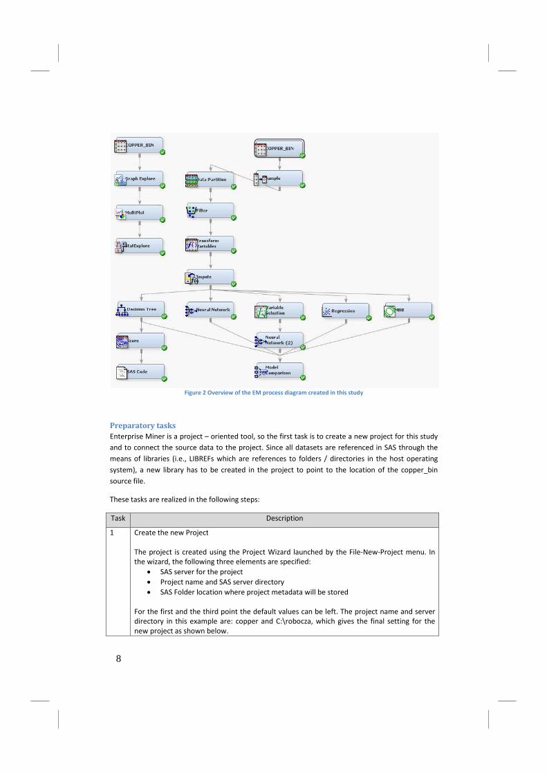
Figure 2 Overview of the EM process diagram created in this study

Preparatory tasks

Enterprise Miner is a project – oriented tool, so the first task is to create a new project for this study

and to connect the source data to the project. Since all datasets are referenced in SAS through the

means of libraries (i.e., LIBREFs which are references to folders / directories in the host operating

system), a new library has to be created in the project to point to the location of the copper_bin

source file.

These tasks are realized in the following steps:

Task Description

1 Create the new Project

The project is created using the Project Wizard launched by the File-New-Project menu. In

the wizard, the following three elements are specified:

• SAS server for the project

• Project name and SAS server directory

• SAS Folder location where project metadata will be stored

For the first and the third point the default values can be left. The project name and server

directory in this example are: copper and C:\robocza, which gives the final setting for the

new project as shown below.

8

2 Connect the source data to the project

1. Create the new Library

The source data used in this example is the copper_bin dataset. First, a new library

has to be created to point to the location (OS folder) of this dataset – the library is

created using the Library Wizard launched by the File-New-Library menu.

2. Create the new Data Source

data source is created using the Data Source Wizard (File-New-Data Source menu).

In the wizard, the following decisions are made:

• A SAS table is selected that becomes the data source (in this example the dataset

copper_bin is used, found in the library created in the previous step)

• The column metadata are defined (such as the roles in the model and

measurement levels of variables). In this step default values of metadata can be

left, as proposed by the Metadata Advisor. Although the metadata could be

corrected here, this will be done and explained in detail in the Sample data step.

• All other settings should be accepted as proposed by the wizard.

3 Create the new Diagram

Using the File-New-Diagram menu, the new diagram called copper is created. The diagram

will be populated with Enterprise Miner nodes to form the process flow as illustrated in

Figure 2.

Sample data

In this step, we start building the process flow by connecting to and possibly sampling the data

source, providing proper metadata for the variables and partitioning the data into training, validation

and testing layers. These tasks are done in the following steps.

9

Task Description

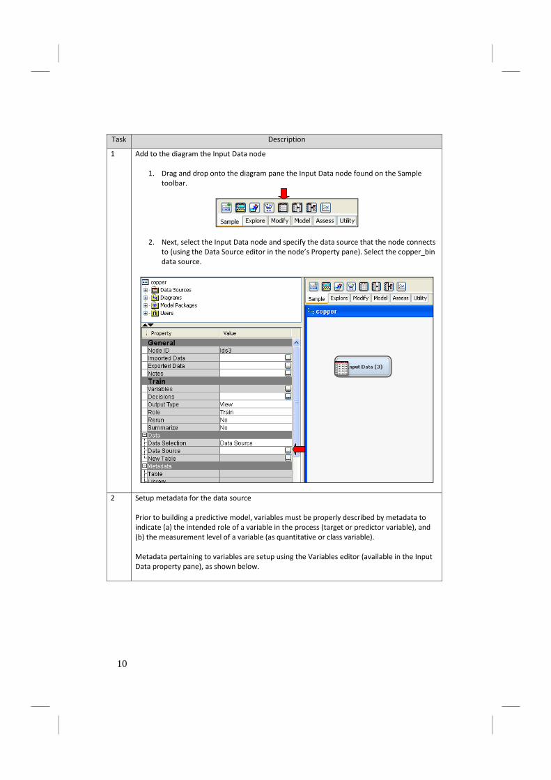
1 Add to the diagram the Input Data node

1. Drag and drop onto the diagram pane the Input Data node found on the Sample

toolbar.

2. Next, select the Input Data node and specify the data source that the node connects

to (using the Data Source editor in the node’s Property pane). Select the copper_bin

data source.

2 Setup metadata for the data source

Prior to building a predictive model, variables must be properly described by metadata to

indicate (a) the intended role of a variable in the process (target or predictor variable), and

(b) the measurement level of a variable (as quantitative or class variable).

Metadata pertaining to variables are setup using the Variables editor (available in the Input

Data property pane), as shown below.

10

The role and measurement level of the copper_bin variables should be specified as follows.

The qbin variable is used as the binary target, the part number and original value of quality

variables are rejected from model building and all other variables are used as predictors with

the interval measurement level (which indicates a quantitative variable).

3 Partition data

Prior to training predictive models, input data must be divided into training, validation and

test partitions. The training partition is used to fit a predictive model to the data, the

validation partition is used to fine-tune parameters of the model in order to avoid model

overfitting Model fine-tuning consists in modification of such parameters of models as depth

of a decision tree or the number of perceptrons in the hidden layer of a neural net, etc. The

test partition can then be used to estimate the expected prediction error for new data.

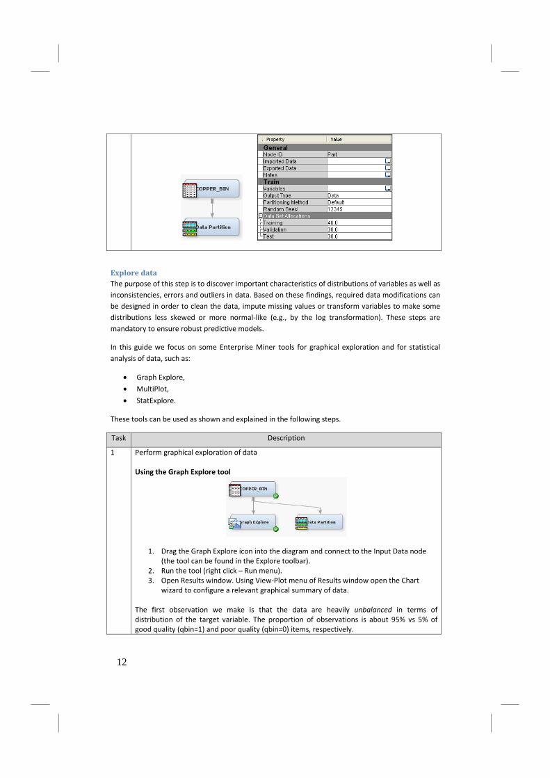
The data is split by connecting the Data Partition node (available in the Sample toolbox) as

shown below.

Data Set Allocations property of the Data Partition node provides the size of partitions (as

percentages of original data); default size can be left as is. The Exported Data property

provides names of the training, validation and test datasets produced by the node.

11

Explore data

The purpose of this step is to discover important characteristics of distributions of variables as well as

inconsistencies, errors and outliers in data. Based on these findings, required data modifications can

be designed in order to clean the data, impute missing values or transform variables to make some

distributions less skewed or more normal-like (e.g., by the log transformation). These steps are

mandatory to ensure robust predictive models.

In this guide we focus on some Enterprise Miner tools for graphical exploration and for statistical

analysis of data, such as:

• Graph Explore,

• MultiPlot,

• StatExplore.

These tools can be used as shown and explained in the following steps.

Task Description

1 Perform graphical exploration of data

Using the Graph Explore tool

1. Drag the Graph Explore icon into the diagram and connect to the Input Data node

(the tool can be found in the Explore toolbar).

2. Run the tool (right click – Run menu).

3. Open Results window. Using View-Plot menu of Results window open the Chart

wizard to configure a relevant graphical summary of data.

The first observation we make is that the data are heavily unbalanced in terms of

distribution of the target variable. The proportion of observations is about 95% vs 5% of

good quality (qbin=1) and poor quality (qbin=0) items, respectively.

12

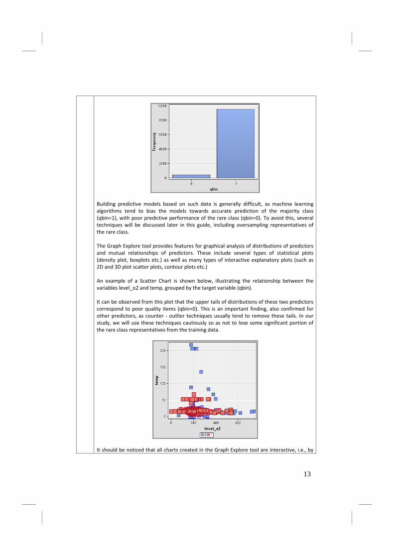
Building predictive models based on such data is generally difficult, as machine learning

algorithms tend to bias the models towards accurate prediction of the majority class

(qbin=1), with poor predictive performance of the rare class (qbin=0). To avoid this, several

techniques will be discussed later in this guide, including oversampling representatives of

the rare class.

The Graph Explore tool provides features for graphical analysis of distributions of predictors

and mutual relationships of predictors. These include several types of statistical plots

(density plot, boxplots etc.) as well as many types of interactive explanatory plots (such as

2D and 3D plot scatter plots, contour plots etc.)

An example of a Scatter Chart is shown below, illustrating the relationship between the

variables level_o2 and temp, grouped by the target variable (qbin).

It can be observed from this plot that the upper tails of distributions of these two predictors

correspond to poor quality items (qbin=0). This is an important finding, also confirmed for

other predictors, as counter - outlier techniques usually tend to remove these tails. In our

study, we will use these techniques cautiously so as not to lose some significant portion of

the rare class representatives from the training data.

It should be noticed that all charts created in the Graph Explore tool are interactive, i.e., by

13

selecting an element on the plot (such as a point or group of points in scatter plot, a bin in

the histogram etc.), corresponding observations in the tabular view of raw data are also

selected. This allows for easy and efficient analysis of observations which contribute to

untypical values in distributions of some variables.

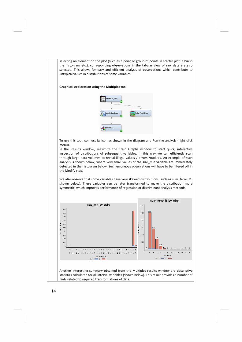
Graphical exploration using the Multiplot tool

To use this tool, connect its icon as shown in the diagram and Run the analysis (right click

menu).

In the Results window, maximize the Train Graphs window to start quick, interactive

inspection of distributions of subsequent variables. In this way we can efficiently scan

through large data volumes to reveal illegal values / errors /outliers. An example of such

analysis is shown below, where very small values of the size_min variable are immediately

detected in the histogram below. Such erroneous observations will have to be filtered off in

the Modify step.

We also observe that some variables have very skewed distributions (such as sum_ferro_f1,

shown below). These variables can be later transformed to make the distribution more

symmetric, which improves performance of regression or discriminant analysis methods.

Another interesting summary obtained from the Multiplot results window are descriptive

statistics calculated for all interval variables (shown below). This result provides a number of

hints related to required transformations of data.

14

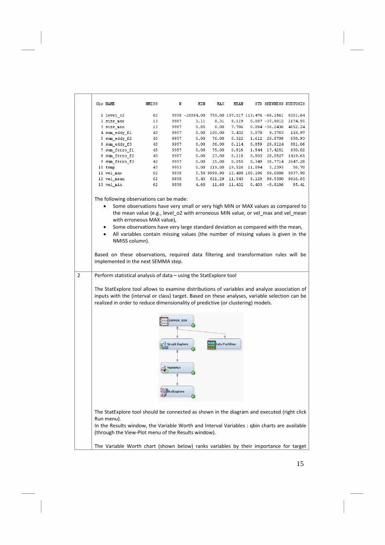
The following observations can be made:

• Some observations have very small or very high MIN or MAX values as compared to

the mean value (e.g., level_o2 with erroneous MIN value, or vel_max and vel_mean

with erroneous MAX value),

• Some observations have very large standard deviation as compared with the mean,

• All variables contain missing values (the number of missing values is given in the

NMISS column).

Based on these observations, required data filtering and transformation rules will be

implemented in the next SEMMA step.

2 Perform statistical analysis of data – using the StatExplore tool

The StatExplore tool allows to examine distributions of variables and analyze association of

inputs with the (interval or class) target. Based on these analyses, variable selection can be

realized in order to reduce dimensionality of predictive (or clustering) models.

The StatExplore tool should be connected as shown in the diagram and executed (right click

Run menu).

In the Results window, the Variable Worth and Interval Variables : qbin charts are available

(through the View-Plot menu of the Results window).

The Variable Worth chart (shown below) ranks variables by their importance for target

15

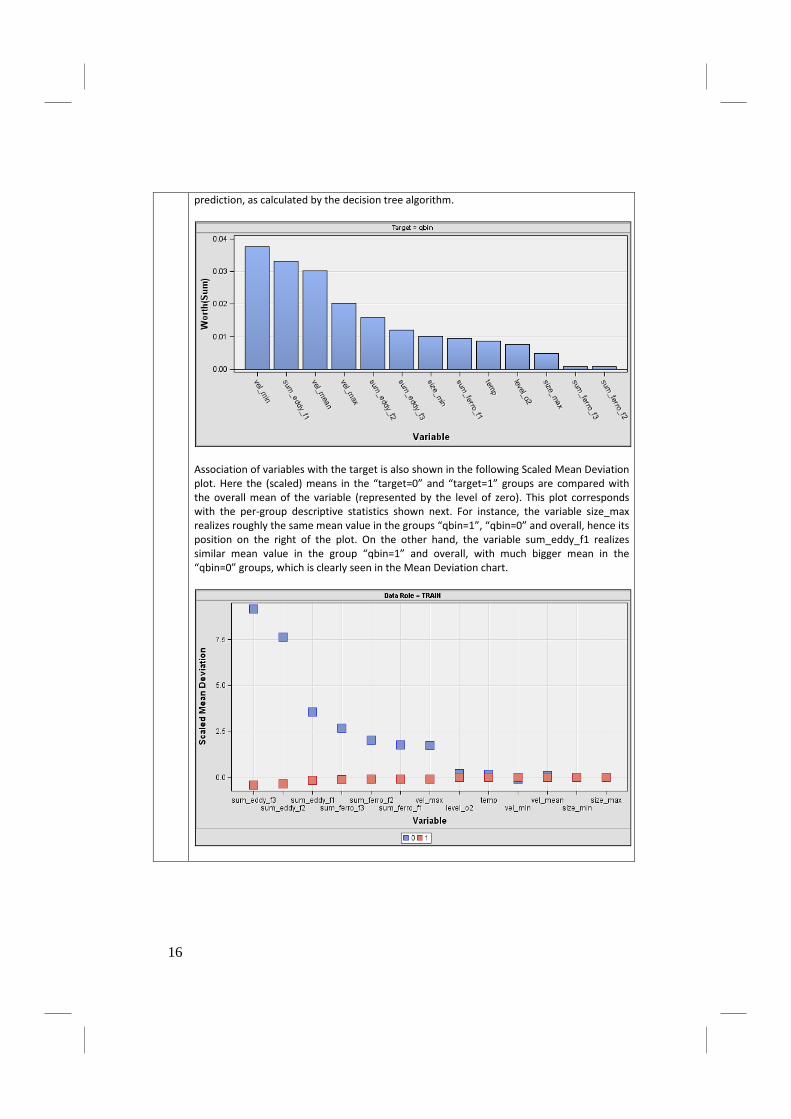
prediction, as calculated by the decision tree algorithm.

Association of variables with the target is also shown in the following Scaled Mean Deviation

plot. Here the (scaled) means in the “target=0” and “target=1” groups are compared with

the overall mean of the variable (represented by the level of zero). This plot corresponds

with the per-group descriptive statistics shown next. For instance, the variable size_max

realizes roughly the same mean value in the groups “qbin=1”, “qbin=0” and overall, hence its

position on the right of the plot. On the other hand, the variable sum_eddy_f1 realizes

similar mean value in the group “qbin=1” and overall, with much bigger mean in the

“qbin=0” groups, which is clearly seen in the Mean Deviation chart.

16

Summarizing, the following conclusions can be drawn from the Explore step:

• The data has heavily imbalanced distribution of target with roughly 5% of the rare class (poor

quality items),

• Some predictors have clearly erroneous observations (such as the negative value of the

level_o2), most of predictors have skewed distributions,

• Most of predictors include outlying observations, these however should be removed with

caution (i.e., only when the value of predictor is beyond physical range of the variable), as

outliers generally correspond to the rare class (poor quality) observations.

These issues will be tackled in the following Modify and Model steps.

Modify data

The purpose of this step is to:

• Remove observations with wrong or outlying values of input variables,

• Transform variables to reduce skewness in distribution,

• Impute missing values.

Transformations of data to reduce skew in distribution bring variables closer to the normal

distribution, which improves performance of predictive models based on the assumption on

normality of features (such as the LDA). Filling in missing data (e.g., based on values in similar

observations or using more sophisticated approach, such as prediction based methods) may improve

performance of regression methods or neural classifiers which otherwise ignore observations in

which missing values occur. (Note that decision tree algorithms accept missing values as legitimate

values of predictors).

In this guide, we demonstrate several features of Enterprise Miner used to modify data, such as

features implemented in the following nodes:

17

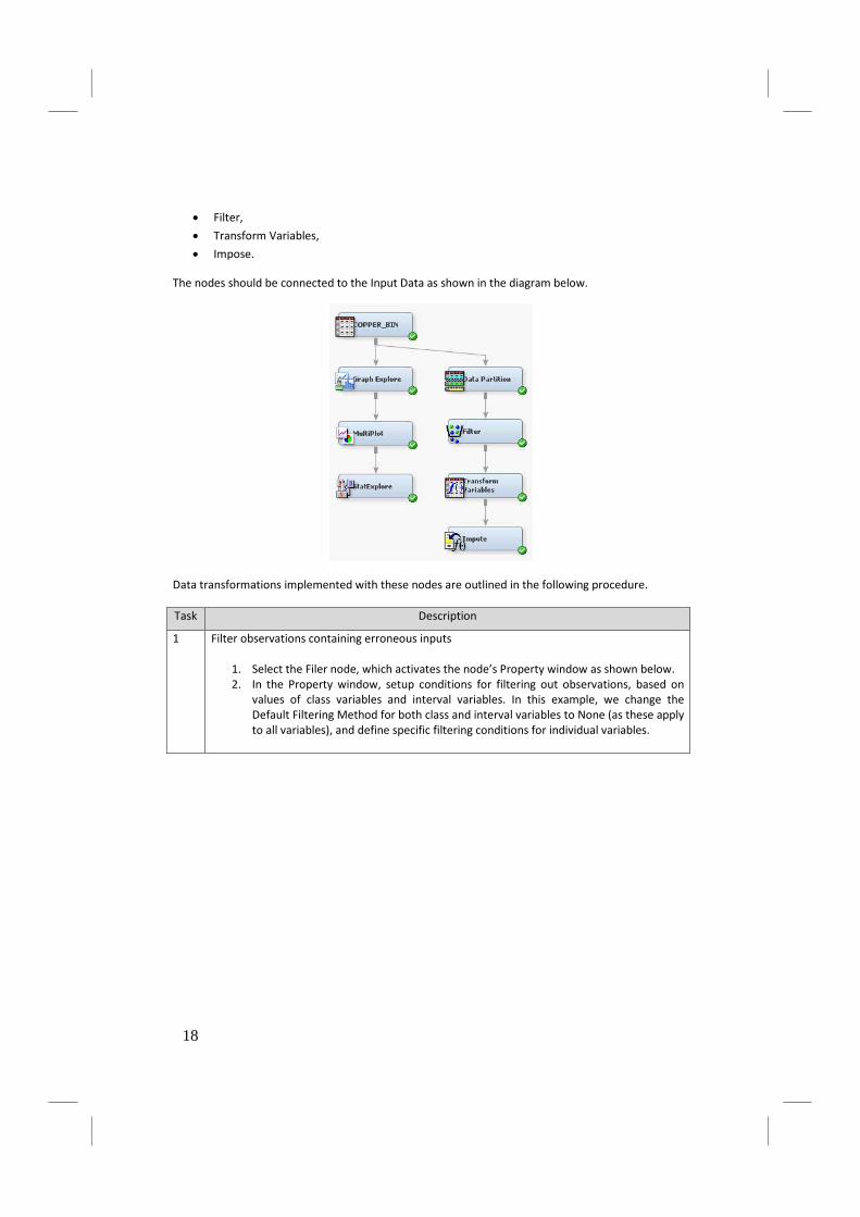
• Filter,

• Transform Variables,

• Impose.

The nodes should be connected to the Input Data as shown in the diagram below.

Data transformations implemented with these nodes are outlined in the following procedure.

Task Description

1 Filter observations containing erroneous inputs

1. Select the Filer node, which activates the node’s Property window as shown below.

2. In the Property window, setup conditions for filtering out observations, based on

values of class variables and interval variables. In this example, we change the

Default Filtering Method for both class and interval variables to None (as these apply

to all variables), and define specific filtering conditions for individual variables.

18

The tool offers several filtering methods, e.g., Standard Deviations from the Mean for

interval variables. This method removes outliers, where outliers are defined by the 3

standard deviations from the mean condition.

In this example, we switch the Default Filtering Method to None. The default Standard

Deviations from the Mean method would remove too many rare case (qbin=0) observations,

as these observations are generally overrepresented in the far ends of distributions of

predictors, as shown in the Explore stage. Thus we manually setup filtering conditions to

remove wrong and preserve feasible albeit outlying data.

We do this using the editor of filtering conditions for interval inputs (the editor is invoked as

indicated by the arrow below).

Next, we specify lower and upper limits for the inputs: level_o2 and vel_max as shown below

(this removes observations with erroneous values in these variables).

19

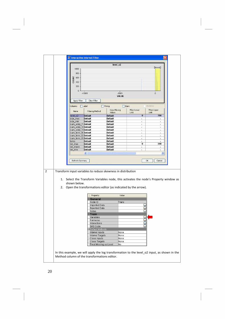
2 Transform input variables to reduce skewness in distribution

1. Select the Transform Variables node, this activates the node’s Property window as

shown below.

2. Open the transformations editor (as indicated by the arrow).

In this example, we will apply the log transformation to the level_o2 input, as shown in the

Method column of the transformations editor.

20

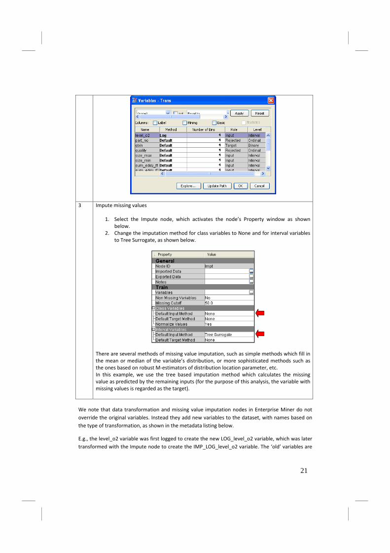
3 Impute missing values

1. Select the Impute node, which activates the node’s Property window as shown

below.

2. Change the imputation method for class variables to None and for interval variables

to Tree Surrogate, as shown below.

There are several methods of missing value imputation, such as simple methods which fill in

the mean or median of the variable’s distribution, or more sophisticated methods such as

the ones based on robust M-estimators of distribution location parameter, etc.

In this example, we use the tree based imputation method which calculates the missing

value as predicted by the remaining inputs (for the purpose of this analysis, the variable with

missing values is regarded as the target).

We note that data transformation and missing value imputation nodes in Enterprise Miner do not

override the original variables. Instead they add new variables to the dataset, with names based on

the type of transformation, as shown in the metadata listing below.

E.g., the level_o2 variable was first logged to create the new LOG_level_o2 variable, which was later

transformed with the Impute node to create the IMP_LOG_level_o2 variable. The ‘old’ variables are

21

rejected from analysis and the modified variables labeled as inputs, i.e., will be used as predictors

(this is done by the Role metadata column).

The metadata can be inspected and modified if necessary using the Metadata node as shown in the

diagram below. This node could be used for manual feature selection, i.e., to include or reject

variables based on association of inputs with the target (see results of the StatExplore node).

In this example we use the Metadata node only for illustration on how transformation nodes work

and hence this node will not be shown in the following diagrams.

Build predictive models

In this step, we will build different predictive models to estimate the target, i.e., to classify the

manufactured items as good or poor quality. We will try:

• Decision trees,

• Neural networks,

• Logistic regression,

22

• Memory based reasoning method (i.e., the nonparametric k nearest neighbours classifier).

We will also demonstrate how feature selection can be realized in Enterprise Miner. Strictly speaking,

this step is not crucial in our study, since the number of variables is relatively small. However in many

real life problems with hundreds or more features, feature selection reducing dimensionality of data

is mandatory, since many noisy features lead to deterioration in model performance and increase

processing time and memory requirements.

Another important issue to consider prior to fitting a predictive model is definition of the criterion for

model selection / comparison. By default, predictive models attempt to minimize the overall

misclassification rate. This does not necessarily guarantee the optimal performance, especially if the

consequences (costs) of the 0�1 and 1�0 misclassification decisions are different. In such studies,

minimization of misclassification costs (or alternatively maximization of profits) might be the right

criterion for model selection. This issue is discussed in the next section on Target profiling.

In this study, we also have to consider the problem of highly imbalanced data (as the poor quality

class is represented by only ca 5% of observations). Predictive models usually demonstrate poor

performance for the rare class. The reasons for this and the methods to tackle the problem are

discussed in the Working with imbalanced data section.

Target profiling

The target profile is used to specify costs of 0�1 and 1�0 misclassifications. Target profiles are also

applied in non binary classification problems, when costs of ci � cj decisions are provided in the form

of the cost matrix, with ci, cj denoting the class labels.

Once defined for the target variable, the target profile is used by the model fitting algorithms to

attempt to minimize the misclassification costs or maximize the overall profit.

The target profile is setup using the procedure outlined below.

Task Description

1 Associate the Target profile with the qbin variable

1. Select the Input Data node, which activates the node’s Property window.

2. In the Property window, open the Decisions editor as shown below. In the Decision

Processing window, click the Build button, which creates the default target profile

for the qbin variable.

23

3. The target event level is selected based on the target level order. The target event

level is later used to define the meaning of sensitivity of the classifier; also the (logit

of) probability modelled by the logistic regression is related to the target event. In

our case, we accept the event level of 1 (which translates into the decision of the

classifier that an item is of good quality; also sensitivity of the model, reported later

in the “Assessment of performance of the models” section will denote probability of

correct recognition of the good quality item).

(If event level of 0 makes interpretation of classifier’s decisions easier, the event

level can be changed by setting the Target level order to Ascending in the metadata

associated with the target variable. Generally, the event level is selected as the first

value in the list of sorted values of the target).

2 Define decision weights

In Decision Weights editor (shown in the following picture), we specify costs (or profits)

associated with particular decisions by the classifier, where:

• DECISION1 means classify as good quality (qbin=1),

• DECISION2 means classify as poor quality (qbin=0),

as indicated by the Decision tab (see the second picture).

In the weights (or profits) matrix shown below, we reflect the following scenario (this

scenario is based on the actual business perspective as seen by the copper company, albeit

the values of profits/costs are fictitious):

• If an actually good quality item (level=1) is classified as good quality (DECISION1),

then the company makes the profit of 10.

• If an actually poor quality item (level=0) is classified as good quality (DECISION1),

then the company makes the profit of -100 (i.e., makes a loss, due to having to pay

high warranty costs to its customer, exceeding prior profits).

• If an item is classified as poor quality (DECISION2), then the company sells the

product as second quality, thus cheaper, and makes the profit of 5, irrespective of

the actual quality.

24

We select the maximize decision function which is consistent with our interpretation of the

values entered as profits (if costs were entered, then the minimize decision function would

have to be selected).

Once the target profile and the weights matrix is associated with the target, subsequent builds of

predictive models will attempt to maximize the profit (or minimize costs) as the criterion for classifier

selection.

Working with imbalanced data

If members of one class are rare in the training data (as the poor quality qbin=0 items are in our

study), then classifiers usually perform poorly for this class. The following reasons make detection of

rare cases challenging:

• A priori probability Pr(c1) of the rare class (denoted c1) is small, as compared with a priori

probabilities of remaining classes. Since the a posteriori (or posterior) probability of this class

is proportional to its a priori probability: ��|��~��|��, where x denotes the

vector of features of an item to classify, then it may be hard to find items x for which Pr(c1|x)

wins among all classes.

• Iterative machine learning algorithms (such as neural nets) tend to fine-tune the weights

towards good recognition of the frequent class. The rules for recognition of the rare class

tend to become very weak as training examples for this class are presented infrequently to

the weights modification algorithm.

25

For these reasons, working with imbalanced data requires special techniques to improve detection of

the rare cases.

In this guide we demonstrate two techniques that are feasible in Enterprise Miner:

• Data oversampling: an artificial training dataset is constructed where the rare cases are

oversampled so that frequencies of the classes are balanced. Obviously, performance of

predictive models is later measured based on the original (i.e., imbalanced) proportions of

classes.

• Boosting recognition of the rare class by the means of decision weights matrix. For instance,

if the classifier tends to classify many poor quality items (level qbin=0) as good quality

(DECISION1), then we may make the classifier avoid the 0�1 misclassification by applying a

high cost of this decision. In this way, we can favour the “pro rare case” decisions which will

boost specificity of models.

Note that this approach is based on the same Decision Weights matrix as used before in the

Target profiling section. However, decision weights defined previously were supposed to

reflect the actual consequences of wrong and correct decisions. Here decision weights are

simply the means to boost recognition of the otherwise “neglected” class.

In this study, we will start with the second approach, as the previously specified Decision Weights

matrix works against the wrong, although likely, 0�1 decisions. This should improve recognition of

the poor quality items. We will verify this supposition by comparing the classifier built using the

decision weights matrix with the original one trained to minimize the overall misclassification rate.

Later in this study, we will also attempt the first method, i.e., we will retrain models based on

oversampled data.

It is generally not clear whether oversampling leads to any significant improvement as compared to

the method based on decision weights, considering the fact that oversampling actually removes data

from the over-represented class (as shown later). Simulation studies indicate that for 3 or more class

recognition problems oversampling seems to be the method of choice, however for binary

classification little improvement is often observed after rare class recognition has already been

boosted by decision weights. The oversampling approach is explained in detail in section Working

with imbalanced data – .

Using predictive modelling nodes

We will build and compare five classifiers:

• Decision tree,

• Neural network (multilayer perceptron),

• Neural network preceded by a variable selection node,

• Logistic regression using forward feature selection method,

• Memory Based Reasoning (MBR), which is a simple nonparametric nearest neighbours

classifier.

To build these classifiers, predictive modelling nodes should be added to the diagram as shown

below.

26

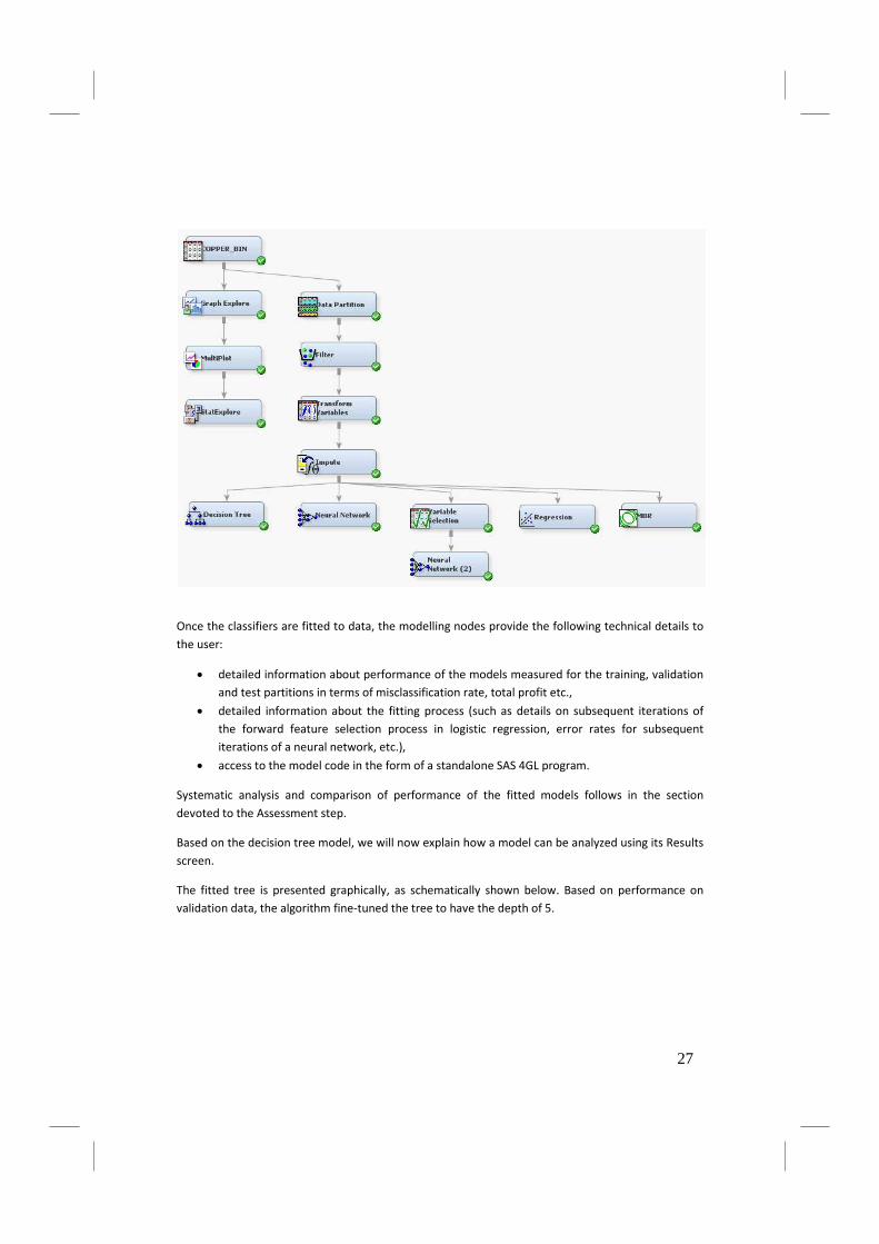
Once the classifiers are fitted to data, the modelling nodes provide the following technical details to

the user:

• detailed information about performance of the models measured for the training, validation

and test partitions in terms of misclassification rate, total profit etc.,

• detailed information about the fitting process (such as details on subsequent iterations of

the forward feature selection process in logistic regression, error rates for subsequent

iterations of a neural network, etc.),

• access to the model code in the form of a standalone SAS 4GL program.

Systematic analysis and comparison of performance of the fitted models follows in the section

devoted to the Assessment step.

Based on the decision tree model, we will now explain how a model can be analyzed using its Results

screen.

The fitted tree is presented graphically, as schematically shown below. Based on performance on

validation data, the algorithm fine-tuned the tree to have the depth of 5.

27

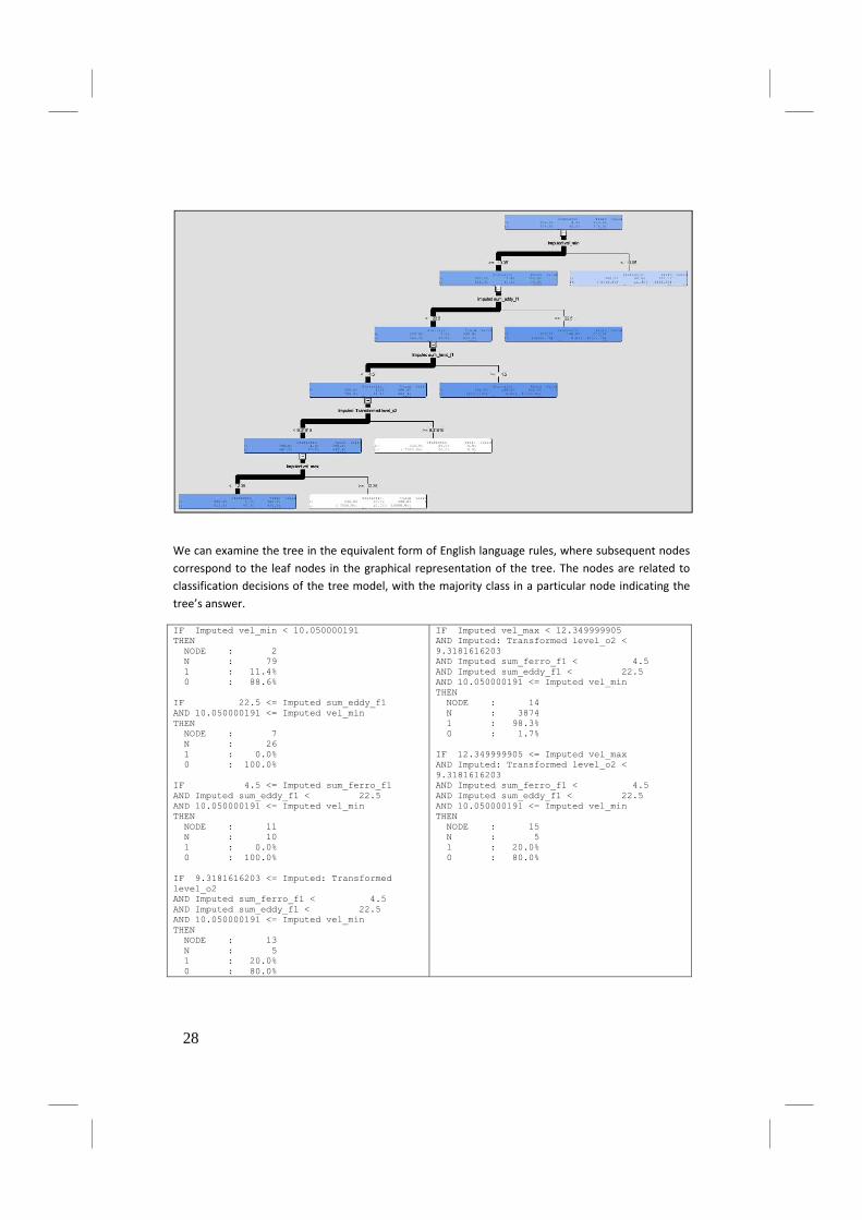
We can examine the tree in the equivalent form of English language rules, where subsequent nodes

correspond to the leaf nodes in the graphical representation of the tree. The nodes are related to

classification decisions of the tree model, with the majority class in a particular node indicating the

tree’s answer.

IF Imputed vel_min < 10.050000191 THEN NODE : 2 N : 79 1 : 11.4% 0 : 88.6% IF 22.5 <= Imputed sum_eddy_f1 AND 10.050000191 <= Imputed vel_min THEN NODE : 7 N : 26 1 : 0.0% 0 : 100.0% IF 4.5 <= Imputed sum_ferro_f1 AND Imputed sum_eddy_f1 < 22.5 AND 10.050000191 <= Imputed vel_min THEN NODE : 11 N : 10 1 : 0.0% 0 : 100.0% IF 9.3181616203 <= Imputed: Transformed level_o2 AND Imputed sum_ferro_f1 < 4.5 AND Imputed sum_eddy_f1 < 22.5 AND 10.050000191 <= Imputed vel_min THEN NODE : 13 N : 5 1 : 20.0% 0 : 80.0%

IF Imputed vel_max < 12.349999905 AND Imputed: Transformed level_o2 < 9.3181616203 AND Imputed sum_ferro_f1 < 4.5 AND Imputed sum_eddy_f1 < 22.5 AND 10.050000191 <= Imputed vel_min THEN NODE : 14 N : 3874 1 : 98.3% 0 : 1.7% IF 12.349999905 <= Imputed vel_max AND Imputed: Transformed level_o2 < 9.3181616203 AND Imputed sum_ferro_f1 < 4.5 AND Imputed sum_eddy_f1 < 22.5 AND 10.050000191 <= Imputed vel_min THEN NODE : 15 N : 5 1 : 20.0% 0 : 80.0%

28

Analyzing the tree model, we can also observe various fit statistics calculated for the training,

validate and test partitions:

We observe that the misclassification rate for the test data (i.e., expected error rate for new data)

equals about 1.5%, and the total profit expected from 3002 items in the test partition equals 25015,

which translates into average profit per item of 8.33. Note that if all the items were actually good

quality and all classification decisions were correct, then the total profit would amount to about 30

thousand. The difference (of ca 5 thousand) is due to

• some poor quality items in the batch (this accounts for ca 0.75K difference),

• the classifier’s errors (these account for majority of the difference, i.e., over 4K).

Another interesting perspective in analysis of the tree model is based on the Classification chart,

where we observe that the rare class (qbin=0) is indeed much more difficult to properly classify,

while items of the frequent class are classified almost perfectly.

Analysis of the tree model also provides information about importance of inputs for prediction of

target, as shown below. This information may be useful for implementation of feature selection

29

rules. It can be observed that the tree selects only the first five variables on top of the list below as

predictors for estimation of the target.

The tree node offers several other interesting methods for analysis of the model, such as e.g., lift

analysis. These methods are however more appropriate for problems where the task consists in

selection of items with the highest probability of event. In our case, the problem consists in quality

prediction of all the items with the criterion to minimize the cost of wrong decisions (or maximize

overall profit).

Similar in-depth analysis of the fitted models is available with other nodes (Neural Network,

Regression, MBR). However, in the next section we will concentrate on comparison of the models in

terms of some simple practical criteria.

Assessment of performance of the models

The purpose of this SEMMA step is to evaluate and compare models in terms of their practical

usefulness. The models can be compared using several criteria such as the profit/loss,

misclassification rate, or using ROC curves or cut-off analysis.

Overall assessment of fitted models is realized with the Model Comparison node, added to the

diagram after the modelling nodes (see diagram below).

30

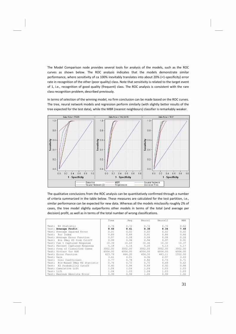
The Model Comparison node provides several tools for analysis of the models, such as the ROC

curves as shown below. The ROC analysis indicates that the models demonstrate similar

performance, where sensitivity of ca 100% inevitably translates into about 20% (=1-specificity) error

rate in recognition of the other (poor quality) class. Note that sensitivity is related to the target event

of 1, i.e., recognition of good quality (frequent) class. The ROC analysis is consistent with the rare

class recognition problem, described previously.

In terms of selection of the winning model, no firm conclusion can be made based on the ROC curves.

The tree, neural network models and regression perform similarly (with slightly better results of the

tree expected for the test data), while the MBR (nearest neighbours) classifier is remarkably weaker.

The qualitative conclusions from the ROC analysis can be quantitatively confirmed through a number

of criteria summarized in the table below. These measures are calculated for the test partition, i.e.,

similar performance can be expected for new data. Whereas all the models misclassify roughly 2% of

cases, the tree model slightly outperforms other models in terms of the total (and average per

decision) profit, as well as in terms of the total number of wrong classifications.

Test: KS Statistic Test: Average Profit Test: Average Squared Error Test: Roc Index Test: Average Error Function Test: Bin 2Way KS Prob Cutoff Test: Cum % Captured Response Test: Percent Captured Response Test: Freq of Classified Cases Test: Divisor for ASE Test: Error Function Test: Gain Test: Gini Coefficient Test: Bin-Based 2Way KS Statistic Test: KS Probability Cutoff Test: Cumulative Lift Test: Lift Test: Maximum Absolute Error

Tree Reg Neural Neural2 MBR 0.76 0.72 0.72 0.70 0.62 8.66 8.41 8.38 8.34 7.68 0.01 0.02 0.02 0.02 0.02 0.89 0.89 0.91 0.86 0.86 0.07 0.08 0.08 0.08 0.26 0.99 0.94 0.94 0.97 0.91 10.39 10.43 10.46 10.32 10.37 5.18 5.16 5.20 5.13 5.17 3002.00 3002.00 3002.00 3002.00 3002.00 6004.00 6004.00 6004.00 6004.00 6004.00 423.79 464.20 454.30 483.11 1552.93 3.61 4.01 4.36 2.97 3.43 0.77 0.78 0.82 0.73 0.71 0.76 0.72 0.72 0.69 0.62 0.80 0.94 0.89 0.92 0.88 1.04 1.04 1.04 1.03 1.03 1.04 1.03 1.04 1.03 1.03 0.99 0.99 1.00 0.99 1.00

31

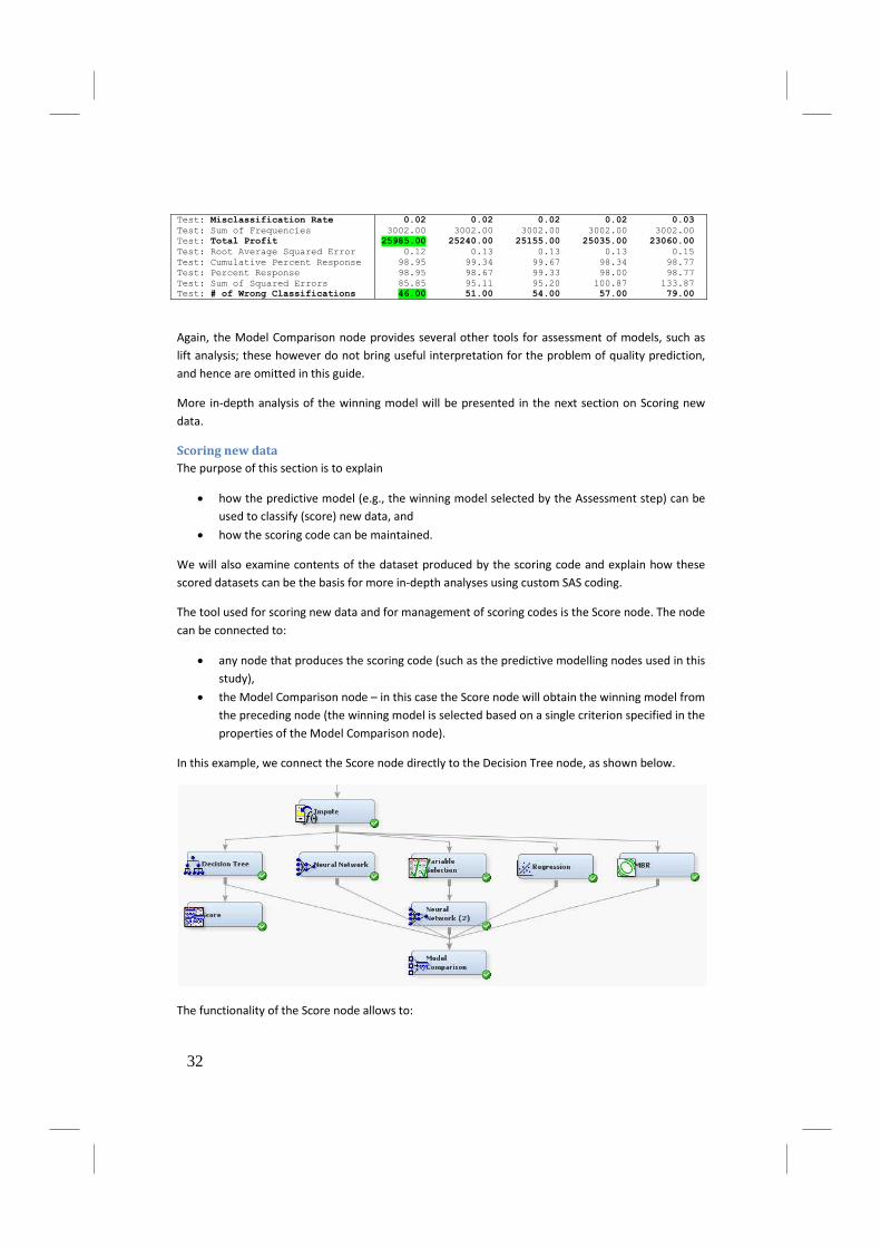
Test: Misclassification Rate Test: Sum of Frequencies Test: Total Profit Test: Root Average Squared Error Test: Cumulative Percent Response Test: Percent Response Test: Sum of Squared Errors Test: # of Wrong Classifications

0.02 0.02 0.02 0.02 0.03 3002.00 3002.00 3002.00 3002.00 3002.00 25985.00 25240.00 25155.00 25035.00 23060.00

0.12 0.13 0.13 0.13 0.15 98.95 99.34 99.67 98.34 98.77 98.95 98.67 99.33 98.00 98.77 85.85 95.11 95.20 100.87 133.87 46.00 51.00 54.00 57.00 79.00

Again, the Model Comparison node provides several other tools for assessment of models, such as

lift analysis; these however do not bring useful interpretation for the problem of quality prediction,

and hence are omitted in this guide.

More in-depth analysis of the winning model will be presented in the next section on Scoring new

data.

Scoring new data

The purpose of this section is to explain

• how the predictive model (e.g., the winning model selected by the Assessment step) can be

used to classify (score) new data, and

• how the scoring code can be maintained.

We will also examine contents of the dataset produced by the scoring code and explain how these

scored datasets can be the basis for more in-depth analyses using custom SAS coding.

The tool used for scoring new data and for management of scoring codes is the Score node. The node

can be connected to:

• any node that produces the scoring code (such as the predictive modelling nodes used in this

study),

• the Model Comparison node – in this case the Score node will obtain the winning model from

the preceding node (the winning model is selected based on a single criterion specified in the

properties of the Model Comparison node).

In this example, we connect the Score node directly to the Decision Tree node, as shown below.

The functionality of the Score node allows to:

32

• Obtain the scoring code from the preceding node. The scoring code can be then managed

outside the Enterprise Miner environment. The scoring code can be exported in the following

languages: SAS 4GL, C, Java, PMML.

• Execute the scoring code against a dataset connected to the Score node. Normally, this

dataset is connected to the Score node using the Input Data node with the metadata role of

Score. Alternatively, the scoring code is applied for the train, validate and test partitions

(these data sets are passed through to the Score node).

In this example, we will use the Score node to classify data in the test partition, since predictive

performance for this partition is a reliable measure of expected performance for new data.

The Exported Data property of the Score node indicates where the results of scoring are placed by

the node. In this example the scored test data is found in the EMWS9.Score_TEST dataset.

The variables in this dataset involved in the classification process are listed by the node in its Results

screen as shown below. These include the predictors used by the tree model as well as variables

produced by the tree node or the score node to provide detailed technical information pertaining to

the classification process.

33

The following variables provide interesting technical information about the process of classification:

D_QBIN Contains the predicted class level (quality of an item). The prediction is

done by the classifier fine-tuned to maximize profit (i.e., built using the

target profile Decision Weights matrix).

I_QBIN Contains the predicted class label, produced by the classifier fine-tuned

to minimize the overall number of misclassified items (i.e., built without

using the target profile Decision Weights matrix). The name given to

this variable by the scoring node is EM_CLASSIFICATION.

EM_EVENTPROBABILITY The probability associated with the classifier’s decision that an item is

good quality.

EM_PROBABILITY The probability of the decision finally made by the classifier. This

probability is estimated as:

EM_PROBABILITY = max(EM_EVENTPROBABILITY, 1- EM_EVENTPROBABILITY)

Given this technical output appended to the results of scoring dataset (i.e., EMWS9.Score_TEST),

further in-depth analysis of the model itself or of the scored data is possible using custom SAS

coding.

To illustrate this, we will post-process results of scoring to calculate the coincidence matrix and the

sensitivity and specificity parameters of the model.

To do this, the SAS Code node is connected to the Score node, as shown below.

In order to compute the coincidence matrix, the following SAS code is placed in the SAS Code node

(the Code Editor is available through properties of this node):

proc freq data=emws9.score_test; tables qbin*d_qbin; tables qbin*i_qbin; run;

34

PROC FREQ is the SAS/STAT procedure used to produce frequency or contingency tables to examine

relationship between two classification variables.

In this example, we use the FREQ procedure to compare:

• the actual quality of copper (qbin) with the quality predicted using the profit maximization

rule (this decision is coded in the d_qbin classifier’s output variable), or

• the actual quality of copper (qbin) with the quality predicted using the misclassification rate

minimization rule (this decision is coded in the i_qbin classifier’s output variable).

The coincidence matrixes summarizing performance of these two classifiers are given below. We also

calculate the total profit and misclassification rates.

The conclusions can be summarized as follows:

• The model based on decision weights indeed realizes higher total profit as compared to the

original classifier (25985 vs. 25015), although the total number of misclassifications is higher

(72 vs. 46).

• Improvement in the total profit is achieved by reducing the number of the costly 0�1

classification errors (from 41 to 30), at the expense of increased 1�0 error rate.

Classifier fine tuned to maximize the total profit

Classifier fine tuned to minimize the misclassification rate

Table of qbin by D_QBIN qbin D_QBIN(Decision: qbin) Frequency| Percent | Row Pct | Col Pct |0 |1 | Total ---------+--------+--------+ 0 | 105 | 30 | 135 | 3.50 | 1.00 | 4.50 | 77.78 | 22.22 | | 71.43 | 1.05 | ---------+--------+--------+ 1 | 42 | 2825 | 2867 | 1.40 | 94.10 | 95.50 | 1.46 | 98.54 | | 28.57 | 98.95 | ---------+--------+--------+ Total 147 2855 3002 4.90 95.10 100.00

Table of qbin by I_qbin qbin I_qbin(Into: qbin) Frequency| Percent | Row Pct | Col Pct |0 |1 | Total ---------+--------+--------+ 0 | 94 | 41 | 135 | 3.13 | 1.37 | 4.50 | 69.63 | 30.37 | | 94.95 | 1.41 | ---------+--------+--------+ 1 | 5 | 2862 | 2867 | 0.17 | 95.34 | 95.50 | 0.17 | 99.83 | | 5.05 | 98.59 | ---------+--------+--------+ Total 99 2903 3002 3.30 96.70 100.00

TOTAL PROFIT 25985

TOTAL PROFIT 25015

TOTAL # OF MISCLASSIFICATIONS 72

TOTAL # OF MISCLASSIFICATIONS 46

These models can also be compared in terms of sensitivity and specificity. These parameters

compare as follows:

35

• model on the left: sensitivity=98.54% , specificity=77.78%

• model on the right: sensitivity=99.83% , specificity=69.63%

Observe that (1-specificity) is the misclassification rate for the rare class (poor quality items): this

parameter was reduced from ca 30% to 22%. This analysis confirms that the decision weights matrix

leads to improvement in recognition of the rare class.

Working with imbalanced data – oversampling technique

Classifiers built using heavily imbalanced training data (i.e., data where some class shows much lower

frequency than other classes) tend to realize low predictive performance of the rare class. We

discussed reasons for this previously (see section Working with imbalanced data) and outlined the

methods feasible in Enterprise Miner to improve recognition of the rare class.

In the previous section, we demonstrated that a properly designed decision weights matrix can be

regarded as a tool to improve recognition of the rare class.

This section is devoted to data oversampling – technique commonly discussed in data mining

literature. The method consists in preparing a sample of data in which frequencies of classes are

more similar to each other than in the original dataset (or even equal), and building a classifier based

on this sample. Doing so, we need to make sure that the classifier does not learn false a priori (or

prior) probabilities of classes, representative for the oversampled data, but completely wrong for the

real data.

Here we explain how this task can be implemented in Enterprise Miner and demonstrate

performance of this approach. In this example, we focus only on oversampling as a method to

improve recognition of the rare class, so the decision weight matrix will not be used, to avoid

combining effects of these two approaches. Hence, we modify the process diagram as shown below

by adding:

• a new Input Data node (note that we will modify the target profile of this node to remove

the effect of non-symmetric decision weights),

• a Sample node (this node needs to be configured to do the actual oversampling).

36

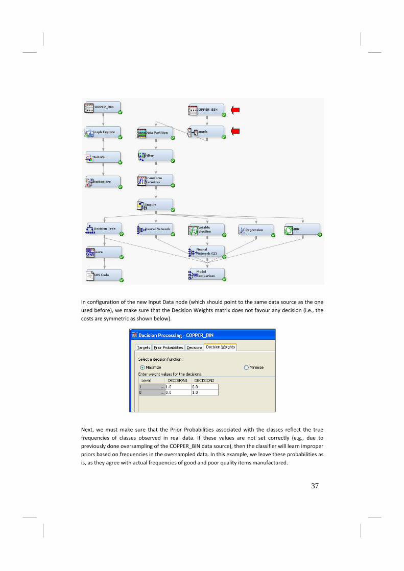
In configuration of the new Input Data node (which should point to the same data source as the one

used before), we make sure that the Decision Weights matrix does not favour any decision (i.e., the

costs are symmetric as shown below).

Next, we must make sure that the Prior Probabilities associated with the classes reflect the true

frequencies of classes observed in real data. If these values are not set correctly (e.g., due to

previously done oversampling of the COPPER_BIN data source), then the classifier will learn improper

priors based on frequencies in the oversampled data. In this example, we leave these probabilities as

is, as they agree with actual frequencies of good and poor quality items manufactured.

37

Next, we configure the Sample node for oversampling. The Sample node can be used to realize very

diverse scenarios of data sampling. In order to make the node do the oversampling properly, it is

essential that the following configuration guidelines are carefully observed.

The required configuration elements of the Sample node (as indicated by arrows on the picture

above) are explained next.

Sample Method: Stratify This setting guarantees that the algorithm will sample

observations from individual classes (or strata) so that user

specified proportions of the classes are achieved in the sample.

These proportions are specified through the Stratified and Level

Based Options properties. (If a variable other than the target

variable should be used for data stratification, then this variable

should be indicated by the Stratification Role in the Variables

metadata).

Stratified Criterion: Level Based This setting informs the algorithm that sample proportions will

be defined in terms of percentages (or counts) pertaining to the

38

fixed level (i.e., value) of the stratification variable. In our case,

the sample will be defined based on the level qbin=0 (i.e., the

rare class).

Level Based Option Level

Selection: Rarest Level

This setting means that the sample proportions specified further

are related to the rare class (i.e., qbin=0).

Level Based Option Level

Proportion: 100

This setting makes the algorithm create the sample with 100%

of the rare class items available in the original dataset (note that

this level, i.e., qbin=0 was chosen previously).

Level Based Option Sample

Proportion: 25

This setting means that the selected level (i.e., qbin=0) will

contribute 25% observations to the sample, with the remaining

75% randomly selected from the frequent class (qbin=1).

The effect of oversampling can be verified through the Results window of the Sample node (shown

below).

Data=DATA Numeric Formatted Frequency Variable Value Value Count Percent qbin 0 0 449 4.49 qbin 1 1 9551 95.51 Data=SAMPLE Numeric Formatted Frequency Variable Value Value Count Percent qbin 0 0 449 25 qbin 1 1 1347 75

It can be observed that the sample indeed contains all (449) poor quality items available in data.

However, in the sample this represents 25% observations, which gives the proportion of the classes

in the sample as 1:3. Thus the proportion is significantly higher as compared to the original

proportion of ca 1:20 (1:19).

Note however that this scenario actually realizes oversampling of the rare class by “undersampling”

of the frequent class. This means that trying to e.g., balance proportions of classes would result in a

yet smaller sample of 2x449 items. So the obvious problem with oversampling is related to losing

(presumably large) part of the training data in the frequent class. It is not clear when this effect of

loosing information through oversampling dominates the desired effect of improvement in rare class

recognition.

(Note that an alternative oversampling scenario could be implemented, where the rare class

observations are actually sampled repeatedly. This is however not implemented in Enterprise Miner

and would required custom SAS coding).

39

In order to observe the effect of oversampling on recognition of the rare class, we execute the SAS

Code node (see diagram above). This calculates the coincidence matrix for the tree algorithm, as

shown below (construction of the coincidence matrix is explained in section Scoring new data).

This result confirms that recognition of rare class improves due to oversampling. However, based on

this results (calculated for oversampled test partition), estimation of the total average profit is not

straightforward, as in reality a different proportion of good/poor quality items is expected.

Classifier built on oversampled data Table of qbin by I_qbin qbin I_qbin(Into: qbin) Frequency| Percent | Row Pct | Col Pct |0 |1 | Total ---------+--------+--------+ 0 | 107 | 28 | 135 | 19.85 | 5.19 | 25.05 | 79.26 | 20.74 | | 93.04 | 6.60 | ---------+--------+--------+ 1 | 8 | 396 | 404 | 1.48 | 73.47 | 74.95 | 1.98 | 98.02 | | 6.96 | 93.40 | ---------+--------+--------+ Total 115 424 539 21.34 78.66 100.00

We also observe that improvement in specificity of the classifier obtained here is slightly better than

improvement achieved with the decision weights matrix (see previous section). However, we should

be cautious trying to interpret this observation as a firm conclusion about higher technical merit of

oversampling. We generally observe that oversampling seems to produce lower total profit measure

than the decision based approach (results not shown here).

Overall performance of the fitted models is additionally reported by the Model Comparison node

through the Event Classification Table (calculated for the train and validation partitions). Below we

compare the oversampled model with the original model (no decision weights used). Based on these

results, specificity of models (i.e., recognition of rare cases) can be estimated as

�� =��

�� + ��

where TN is the number of True Negatives and FP is the number of False Positives summed up for

train and validate partitions. We generally observe higher specificity for oversampled models,

although at the price of deterioration in models’ sensitivity (=TP/(TP+FN)), where TP is the number of

True Positives and FN is the number of False Negatives (again summed up for train and validation

partitions).

40

MODEL BASED ON OVERSAMPLED DATA Event Classification Table Model Selection based on Test: Average Profit (_TAPROF_) Model Data False True False True Node Model Description Role Target Negative Negative Positive Positive Tree Decision Tree TRAIN qbin 4 132 47 535 Tree Decision Tree VALIDATE qbin 5 92 43 399 Neural Neural Network TRAIN qbin 9 136 43 530 Neural Neural Network VALIDATE qbin 12 88 47 392 Neural2 Neural Network (2) TRAIN qbin 2 128 51 537 Neural2 Neural Network (2) VALIDATE qbin 3 88 47 401 Reg Regression TRAIN qbin 6 123 56 533 Reg Regression VALIDATE qbin 6 88 47 398 MBR MBR TRAIN qbin 2 97 82 537 MBR MBR VALIDATE qbin . 62 73 404

MODEL BASED ON ORIGINAL DATA Event Classification Table Model Selection based on Test: Average Profit (_TAPROF_) Model Data False True False True Node Model Description Role Target Negative Negative Positive Positive Tree Decision Tree TRAIN qbin 11 114 66 3808 Tree Decision Tree VALIDATE qbin 3 100 34 2862 Neural Neural Network TRAIN qbin 8 105 75 3811 Neural Neural Network VALIDATE qbin 4 91 43 2861 Neural2 Neural Network (2) TRAIN qbin 7 110 70 3812 Neural2 Neural Network (2) VALIDATE qbin 7 97 37 2858 Reg Regression TRAIN qbin 11 97 83 3808 Reg Regression VALIDATE qbin 7 91 43 2858 MBR MBR TRAIN qbin 0 72 108 3819 MBR MBR VALIDATE qbin 0 62 72 2865

41

PART II Data Warehousing

The purpose of this practical guide to data warehousing is to

• learn how online analytical processing (OLAP) methods and tools can be used to perform

multidimensional analysis of data,

• get hands-on experience and skills in using MS SQL Server Integration Services (SSIS) and

Analysis Services (SSAS) tools for building Extract-Transform-Load (ETL) processes and for

building multidimensional data cubes.

The task solved in this example consists in building a multidimensional cube for analysis of student

notes at a university (notes from our University were used). The tool will allow to investigate

interesting relationships as to how student notes depend on various characteristics of students,

teachers, type of course, etc., and how this changes over time. Examples of questions easily

answered with the tool built in the lab might be: ‘Are older teachers more strict than younger

teachers?’, or ‘Are winter semesters harder than summer semesters?’.

This guide is organised as follows:

• First, an overview of the task is given, including description of the source (input) data,

naming the major steps in data processing and outlining the structure of the

multidimensional cube to be created.

• Secondly, required ETL and multidimensional data modelling steps are presented in detail.

• Finally, the MS SSIS and SSAS tools to be used for building ETL processes and for

multidimensional modelling of data are presented in the tutorial-like fashion.

Overview of this Guide

The source data used in the lab contain notes obtained over five subsequent years by a group of

students of the Faculty of Electronic Engineering. Some attributes of students, teachers, and courses

are also included. The data is provided in the form of five text files: notes.csv, students.csv,

teachers.csv, course_group.csv, teacher_title.csv. Samples of these files are shown in Table 2 through

Table 6.

The purpose of the class is to build an OLAP solution (a data warehouse and a multidimensional

cube) for analysis of student notes. This will be realized by building multidimensional model of the

data with the column note used as the fact variable and the remaining columns used as dimensions

(dimension attributes).

The task will be realized in following steps:

1. Building ETL process,

2. Building multidimensional model of data,

3. Building multidimensional cube.

42

Table 2 Sample of the notes table

Table 3 Sample of the students table

Table 4 Sample of the teachers table

Table 5 Sample of the course_group table

Table 6 Sample of the teacher_title table

Step 1 Building ETL process

Prior to loading data into the data warehouse, errors and/or inconsistencies in the data should be

fixed. This is the purpose of Extract-Transform-Load (ETL) scripts. In our source data, several types of

inconsistencies can be observed, e.g.,

• Missing or illegal values in some columns (e.g., illegal values of note),

• Inconsistent and/or unclear coding conventions (e.g., student’s gender and teacher’s

gender),

• Problems with foreign key (FK) – primary key (PK) relationships between the fact table and

dimension tables (explained in the next section).

Another purpose of the ETL scripts is to modify the structure of the data by deriving new variables

and / or new tables to form interesting new dimensions. Examples of these may include the workload

table (shown in Figure 4), not available in the source data but calculated in the ETL stage. Generally,

restructuring the data at the ETL stage is supposed to simplify multidimensional modelling of data

(the task realized as Step 2).

43

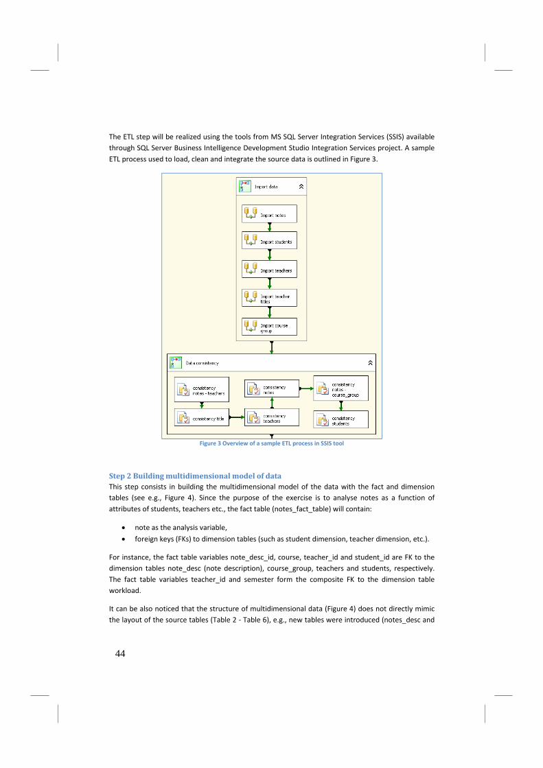
The ETL step will be realized using the tools from MS SQL Server Integration Services (SSIS) available

through SQL Server Business Intelligence Development Studio Integration Services project. A sample

ETL process used to load, clean and integrate the source data is outlined in Figure 3.

Figure 3 Overview of a sample ETL process in SSIS tool

Step 2 Building multidimensional model of data

This step consists in building the multidimensional model of the data with the fact and dimension

tables (see e.g., Figure 4). Since the purpose of the exercise is to analyse notes as a function of

attributes of students, teachers etc., the fact table (notes_fact_table) will contain:

• note as the analysis variable,

• foreign keys (FKs) to dimension tables (such as student dimension, teacher dimension, etc.).

For instance, the fact table variables note_desc_id, course, teacher_id and student_id are FK to the

dimension tables note_desc (note description), course_group, teachers and students, respectively.

The fact table variables teacher_id and semester form the composite FK to the dimension table

workload.

It can be also noticed that the structure of multidimensional data (Figure 4) does not directly mimic

the layout of the source tables (Table 2 - Table 6), e.g., new tables were introduced (notes_desc and

44

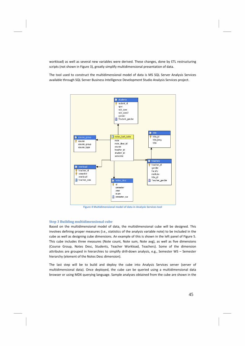
workload) as well as several new variables were derived. These changes, done by ETL restructuring

scripts (not shown in Figure 3), greatly simplify multidimensional presentation of data.

The tool used to construct the multidimensional model of data is MS SQL Server Analysis Services

available through SQL Server Business Intelligence Development Studio Analysis Services project.

Figure 4 Multidimensional model of data in Analysis Services tool

Step 3 Building multidimensional cube

Based on the multidimensional model of data, the multidimensional cube will be designed. This

involves defining proper measures (i.e., statistics of the analysis variable note) to be included in the

cube as well as designing cube dimensions. An example of this is shown in the left panel of Figure 5.

This cube includes three measures (Note count, Note sum, Note avg), as well as five dimensions

(Course Group, Notes Desc, Students, Teacher Workload, Teachers). Some of the dimension

attributes are grouped in hierarchies to simplify drill-down analysis, e.g., Semester WS – Semester

hierarchy (element of the Notes Desc dimension).

The last step will be to build and deploy the cube into Analysis Services server (server of

multidimensional data). Once deployed, the cube can be queried using a multidimensional data

browser or using MDX querying language. Sample analyses obtained from the cube are shown in the

45

right panel of Figure 5, where course-work notes (CW) are compared with exam notes (E) in terms of

the average note (Note Avg) and the number of notes (Note Count), etc.

The tool used to design structure of the multidimensional cube and to build and deploy the cube is

Analysis Services (available in SQL Server Business Intelligence Development Studio Analysis Services

project).

Figure 5 Structure of the multidimensional cube for analysis of notes (left), and sample results of analysis produced from

the cube (right)

Tasks in Detail

Task Description

1 Import source data

Using MS VS Integration Services project, load the source files notes.csv, students.csv,

teachers.csv, course_group.csv, teacher_title.csv into MS SQL database.

Meaning and type of each column is explained below.

Table notes

semester Semester number

Integer in range 1..10

year Calendar year

Integer in range 1980..

course Id of course

Text, up to 10 characters in length

46

teacher_id Id of a teacher who granted a note to a student


note A note obtained by a student in a course

Real value, legal values: 2, 3.0, 3.5, 4.0, 4.5, 5.0, 5.5

exam Value ‘E’ identifies a note obtained in an exam, empty value identify notes

based on course-work performance of a student.

student_id Id of a student who received the note


Table students

spec Specialization of the student (AIR – Automatics & Robotics; EIT –

Electronics & Telecommunication; INF – Computer Engineering)

Text, 3 characters in length

sub_spec Sub-specialization within specialization groups


sub_spec2 Some (rare) sub-specializations are further split into groups defined by

this value. For most sub-specializations this column is empty.


gender Gender of a student

‘K’ – female, ‘M’ – male

student_id Id of a student, PK of this table


Table teachers

teacher_id Id of a teacher, PK of this table


gender Gender of a teacher

1 – male, 2 – female

faculty Id of the Faculty the teacher is affiliated with (value of 4 denotes Faculty

of Electronic Engineering)


institute Id of the Institute the teacher is affiliated with


title_id Id of teacher’s title, used to relate to the teacher_title table


Table course_group

Course Id of a course, PK of this table


course_group 1 – science and technical courses

2 – sports

3 – foreign languages

4 – social science and management courses

Table teacher_title

title_id Id of teacher’s title, PK of this table


title_long Teacher’s full title


Title Teacher’s short title


47

2 Fix data value inconsistencies / unclear coding conventions

Some columns contain wrong values (e.g., note = 0 or 1), these values should be removed.

Some columns also contain missing values, these should be filled in with some meaningful

data (e.g., empty exam column can be filled in with text ‘CW’ (course work)). Empty values

interpreted as information not available should be changed into text ‘unknown’ or ‘?’, etc.

Gender in teachers and student tables should be coded consistently using symbols clear to

end user.

3 Fix consistency of relationships between tables

Consistency of foreign key – primary key (PK) relationships between tables should be

verified, and, if needed, corrected. For instance, teacher_id in notes table is FK to teachers

table. However, source data is not consistent and this relationship is broken as some values

of FK (teacher_id) in notes table are missing in teachers table. The way to correct this is to

add the missing teacher_id entities to the teachers table. All remaining attributes for these

teachers should be coded as unknown (gender, faculty, institute, title).

The same procedure should be carried out for FK – PK relationships between other tables

(notes – course_group, etc., see Figure 4).

4 Derive new dimension attributes

Several interesting attributes are not directly available in source data, e.g., semester type

(winter semesters vs summer semesters). Such new columns should be derived, which later

allows to add new interesting dimension attributes to the cube.

Proposed new attributes:

• Semester type (winter/summer semesters based on whether semester number is

odd/even)

• Academic year of studies (semesters 1,2 – 1st

year, semesters 3,4 – 2nd

year, etc.)

• Course type – based on the last character of the course symbol (W=Lecture, L=lab,

P=Project, S=Seminar, C=Exercise).

5 Derive workload table (workload dimension)

A new dimension that describes per-semester workload of teachers (and/or workload of

students) should be derived. Workload can be defined as the number of notes a teacher

grants to the students in a given semester, or, alternatively, as the number of different

courses a teacher gives in a semester. The teacher workload table should be created with

the columns teacher_id and semester used as the composite PK.

6 Restructure the fact table notes

The fact table should include only the fact variable (note) and FKs to dimension tables (as in

Figure 4). This can be achieved by moving non-FK columns from the fact table to a separate

table (denoted in Figure 4 as notes_desc) and placing the FK to this table in the fact table

(denoted in Figure 4 as notes_desc_id).

7 Create a multidimensional cube

Using MS VS Analysis Services project, a cube should be designed with the notes fact table

48

and dimension tables pertaining to students, teachers, courses, teacher workload, and other

notes description (such as those created in task 2).

8 Edit measures in the cube

The cube should allow for analysis of the following statistics: the number of notes and the

average note. Thus, the measures in the cube should include sum of notes and count of

notes. A calculated member average note should be then defined for the cube, based on

ratio of these two measures.

9 Edit dimensions

Edit all the dimensions (teacher, student, course, notes descriptions and workload

dimension) by adding relevant attributes. Proposed structure of dimensions is shown in

Figure 5. Related dimension attributes should be grouped into drill-down hierarchies, e.g.,

Specialization hierarchy (Figure 5), which groups Spec�Sub Spec�Sub Spec2 attributes.

Notice: good practice should be observed to hide in the cube structure dimension attributes

used as levels of hierarchies.

10 Build and deploy the cube

Once designed, the cube should be deployed on the instance Analysis Services.

The cube is ready to be browsed with an OLAP viewer or queried using MDX language.

11 Analyze the cube and demonstrate some interesting relationships / trends pertaining to

notes at our Faculty.

How-To Procedures and Hints

The purpose of this part is to:

• explain how subsequent tasks can be realized with MS SQL Server Integration Services (SSIS)

and Analysis Services (SSAS),

• provide some hints and ideas on how inconsistencies in source data can be corrected.

Hint Problem and solution

1 How to import source csv files to MS SQL database?

1. In SQL Server Business Intelligence Development Studio create new Integration Services

project.

2. Create new Flat File Connection Manager (right click in Connection Manager pane). Edit

this Connection Manager to provide location of the source file as well as formatting

details (such as column delimiters, etc.). Care should be taken to specify the proper type

of each column – compliant with the information detailed in Task 1.

3. Create new OLE DB Connection Manager. This Connection Manager is used to specify

name of the database used to store imported tables.

4. Create new Data Flow Task (drag and drop Data Flow icon from toolbox onto the Control

49

Flow pane).

5. Put Flat File Source into this Data Flow Task and specify the appropriate Flat File

Connection Manager.

6. Put OLE DB Destination into this Data Flow Task and connect Flat File Source to this OLE

DB Destination. Edit the OLE DB Destination to specify right OLE DB Connection Manager

and request New table to store imported data. Notice that this will create the

destination DB table, with the generated SQL CREATE TABLE statement shown after

pressing the New (table or view) button. It should be verified that the name of the

destination table and types of columns are correct (the name of the destination table is

taken after the name of the OLE DB Destination tool).

7. To import source csv file into the DB table, run the Data Flow Task (right click on its

icon).

Repeat steps 2,4-6 of this procedure for the remaining source files. As a result, five Flat File

Source Connection Managers, and one OLE DB Connection Manager will be created, as

shown below. The Data Flow Tasks created can be grouped using Sequence Container (as

shown in Figure 3).

Notice

Care should be taken how null values in source tables are loaded using Flat File (FF) Source

tool. When the FF Source option “Retain null value” is checked, nulls (coded as ,, in csv files)

will be loaded as NULL into the database. This makes it possible to use constructs like WHERE

teacher_is IS NULL or expressions like ISNULL(teacher_id), etc. (see Hint 2).

2 How to clean imported data / modify wrong values / fill in null values?

Using Data Transformation tools in Data Flow Task

New columns can be derived or existing columns can be conditionally modified using Derived

Column in the data transformation flow, as shown below. The expression shown in this

example is used to overwrite null values in the exam column with an explicit symbol of

course-work notes (“CW”, as opposed to exam notes, coded explicitly by “E”).

Rows can be conditionally deleted from a table using Conditional Split transformation.

Using explicit SQL code

Data cleaning transformations can be alternatively written as SQL scripts placed in Execute

50

SQL Task (elements in Control Flow). All data consistency elements shown in Figure 3 are

examples of this approach. For instance, below is a simple script used to recode teacher’s

gender (SQL Task consistency teachers in Figure 3):

UPDATE teachers SET gender = CASE WHEN gender = '1' THEN 'M' WHEN gender = '2' THEN 'F' ELSE '?' END

3 How to fix foreign key – primary key relationships between tables

The problem will be explained on the example of the dimension teachers (FK – PK

relationship between notes fact table and teachers table).

Verification of consistency of FK – PK relationship

It should be checked if any of values of the FK (teacher_id) in the fact table are missing in the

dimension table, if so (as in our source data) – the relationship is broken.

The idea of SQL code used for verification of the relationship is given below.

SELECT n.teacher_id FROM notes as n LEFT JOIN teachers AS t ON n.teacher_id = t.teacher_id WHERE (t.teacher_id IS NULL) GROUP BY n.teacher_id

Correction of inconsistent relationship

Teacher ids missing from the teachers table should be added to teachers dimension, forming

entities with the remaining columns (teacher gender, etc.) filled with values coding

‘information not available’.

The idea of an SQL script to correct broken relationships is given below.

INSERT INTO teachers SELECT n.teacher_id, ‘?’ AS gender, etc... FROM notes as n LEFT JOIN teachers AS t ON n.teacher_id = t.teacher_id WHERE (t.teacher_id IS NULL) GROUP BY n.teacher_id

4 How to create dimensions based on non-FK columns of the fact table

Method 1

The idea is to create a new dimension table with non-FK columns of the fact table (such as

e.g., semester, etc.; this table is named notes_desc in Figure 4). FK to this table will be placed

in the fact table in place of the columns in this new dimension (these columns will be

removed from the original notes table).

The first step is to create a temporary (aggregate) notes table with the id used as the PK in

the new dimension table and FK in the new fact table. The table will be then split into the

notes fact table and the new dimension table.

The idea of the first step is given below.

SELECT IDENTITY (bigint, 1, 1) AS id,

51

all remaining columns of the fact table... INTO notes_tmp FROM notes

Then the temporary table should be split into the new dimension table:

SELECT id , semester, etc. INTO notes_desc FROM notes_tmp

and into the fact table (notice that only the fact variable and FKs to dimension tables are

being selected):

SELECT note, id AS note_desc_id, remaining FKs to other dimension tables INTO notes_fact_table FROM notes_tmp

The multidimensional model of data formed in this way is shown in Figure 4.

Method 2

The idea is to create separate dimension tables for each of the non-FK column of the fact

table while using this column in the fact table as the FK to the newly created dimension. The

idea will be explained using the semester column as an example.

The code to create new semester dimension:

SELECT DISTINCT semester, other semester-related columns... FROM notes

The new dimension table can be created either physically in the database (ETL script), or as

an named query in Analysis Services data source view.

5 How to create a multidimensional cube?

1. In SQL Server Business Intelligence Development Studio create new Analysis Services

project.

2. Create a new data source (right click on Data Sources in Solution Explorer), pointing at

the database created in the ETL stage. Consider selecting service account for

impersonation information.

3. Create a new data source view (right click on Data Source Views), using the data source

created in the previous step. Create logical FK-PK relationships between the fact table

and the dimension tables (right click on a table, select New Relationship, specify fact

table as the source (foreign key) table and a dimension table as the destination table).

An exemplary data source view is shown below.

52

4. Create a new cube (right click on Cubes in Solution Explorer). Use the table notes as the

measure group (i.e., fact) table, and remaining tables as dimension tables.

The cube can now be built and deployed in Analysis Services instance. However, to make the

cube fully functional, measures stored in the cube as well attributes and properties of

dimensions should be edited (see Hints 6, 7).

6 How to add/edit measures stored in the cube?

To add a new measure, right click on the Measures pane in the cube designer. When

defining the measure, specify proper usage for the measure (such as sum or the number of

notes, which defines how the fact variable should be aggregated when stored in the cube).

See also the AggregateFunction property of the measure.

Notice that only distributive measures can be defined as cube measures (such as sum or

count of values of the fact variable). To provide a definition of non-distributive algebraic

measure (such as the average), a calculated member should be defined for the cube (Hint 7).

7 How to add a calculated member to the cube?

A calculated member allows to add an algebraic formula based on measures stored in the

cube (e.g., average note based on sum and count of notes). To add a calculated member,

select Calculations tab in the cube designer. Then in the right panel define name of the

calculated member and an expression used to calculate it. E.g., the following expression

calculates the mean note based on the two cube measures (see also left panel of Figure 5):

[Measures].[Note Sum]/[Measures].[Note Count]

Notice that while defining the formula, names of cube measures can be dragged from the

Metadata pane of Calculations editor and dropped onto the Expression editor.

8 How to edit dimensions?

53

In dimensions editor, the following properties of dimensions are specified:

• List of attributes of the dimension,

• Drill-down hierarchies in the dimension,

• Properties of attributes related to visibility, sort order, discretization method, etc.

1. To enter dimension designer, in cube designer expand the given dimension in question

(in Dimensions pane), then select command Edit dimension.

2. To design attributes of a dimension, drag and drop a column name to be used as an

attribute from the Data Source View pane of dimension designer onto the Attributes

pane.

3. To create drill-down hierarchies, drag attributes to be grouped onto the Hierarchies

pane, as in the example shown below (Specialization hierarchy of Students dimension –

see Figure 5).

4. For attributes included in a hierarchy, define attribute relationships, as shown in the

example below (use Attribute Relationships tab of dimension designer).

5. To hide some attributes of a dimension, i.e., make them invisible for the user in OLAP

browser, set the AttributeHierarchyVisible property of the attribute to False. For clarity

of the multidimensional model presented to the user, attributes included in levels of drill

down hierarchies are generally not shown as dimension attributes (see e.g., the Students

dimension in Figure 5).

6. If members of an attribute are sorted improperly in the OLAP browser, the sort order

can be changed using OrderBy attribute property.

7. For attributes with a large number of members (different values), such as the workload

dimension, consider setting the DiscretizationMethod property (and related

DiscretizationBucketCount property). This leads to automatic grouping of the large

number of values into buckets and improves clarity of presentation, as shown below.

54

9 How to build / deploy / browse the cube

Once designed, the cube can be built and installed on the instance of Analysis Services

(server of multidimensional databases). To do this, use Build � Deploy menu command in BI

Development Studio.

To perform data analysis using the cube, a multidimensional OLAP browser built into the

development environment can be used. To launch the browser, open MS SQL Management

Studio, connect to Analysis Services, right click the cube name and select the Browse

command.

55

Further Reading

Data Mining

J. Han, M. Kamber, Data Mining: Concepts and Techniques, Second Edition. Elsevier 2006.

T. Hastie, R. Tibshirani, J. H. Friedman, The Elements of Statistical Learning: Data Mining, Inference,

and Prediction. Springer 2009.

D.Larose, Data Mining Methods and Models. Wiley 2006.

S. Theodoridis, K. Koutroumbas, Pattern Recognition. Academic Press 2006.

Getting Started with SAS Enterprise Miner 6.1. SAS Institute 2009. [Electronic document available at

www.sas.com]

Data Warehousing

W. Inmon: Building the data warehouse, Wiley 2005.

F. Silvers: Building and maintaining a data warehouse, CRC Press 2008.

R. Kimball, J. Caserta, The Data Warehouse ETL Toolkit, Wiley Publishing, 2004.

E. Thomson, OLAP Solutions. Building Multidimensional Information Systems, John Wiley & Sons,

Inc.,2002.

56

application programming: data mining and data warehousing ... · pdf filedata mining and data...

Documents