applications of elliptic operators and the atiyah singer index

APPLICATIONS OF ELLIPTIC OPERATORS AND THEATIYAH SINGER INDEX THEOREM

MARTIN BENDERSKY

Contents

1. Review of Differential Geometry 2

2. Definition of an Elliptic Operator 5

3. Properties of Elliptic Operators 7

4. Example of an Elliptic Operator 9

5. Example: The Euler Characteristic 12

6. Example: The Signature Invariant 14

7. A Theorem of Atiyah, Frank and Mayer 18

8. Clifford Algebras 20

9. A Diversion: Constructing Vector Fields on Spheres using

Clifford Algebras 23

10. Topological Invariants of the Index. The Atiyah Singer

Index Theorem 26

11. Borel Hirzebruch Theory and Characteristic Classes 30

12. Verification of the Index Theorem for Dχ 33

13. The Index of DS is the Hirzebruch L-genus 36

14. The Hirzebruch Riemann Roch Theorem 39

References 43

Date: May 3, 2006.1

2 MARTIN BENDERSKY

1. Review of Differential Geometry

References for this material are [ST], [S] or any reasonable differential

geometry text.

We first recall the definition of a locally trivial vector bundle, over

a pointed space X, ξ : F → E → X. E is called the total space and

F = π−1(x) ≈ F n,F = R or C.

We assume X =⋃Ui with ξ|Ui

is trivial. What this means is that

there is a diagram

E|Ui

Ti−→ F n × Ui

↓yπ

Ui = Ui

On the intersections there are the maps

λij = T−1i Tj : F n×Ui

⋂Uj → F n×Ui

⋂Uj which induce maps (also

denoted λij) Ui

⋂Ujλi,j−→ F (n) (F (n) is O(n) if F = R, U(n)if F = C).

The λij satisfy the following composition laws:

(1.1)

• (1) λik = λij λjk on Ui

⋂Uj

⋂Uk

• (2)λii = identity

• (3)λij = λ−1ji

• (4) λi,j is a continuous map from Ui

⋂Uj to F (n)

Notation 1.2.

• X will denote an n dimensional, C∞, compact, closed, oriented man-

ifold.

• rj : Rn → R denotes the j-th coordinate function. In particular ∂∂rj

is

the usual partial with respect to the j-th coordinate.

• xj denotes rj ϕ where ϕ : U → Rn is a local chart, U ⊂ X.

• C(X,x,R) denotes the C∞ functions from some neighborhood of x ∈X to R. Notice that xj may be viewed as an element of C(X,x,R).

• C(X,R) denotes the C∞ global functions f : X → R. More generally

C(X,Y) denotes C∞ functions from X to Y.

Definition 1.3. A tangent vector υ, at x ∈ X is a map υ : C(X,x,R) →R such that

APPLICATIONS OF ELLIPTIC OPERATORS AND THE ATIYAH SINGER INDEX THEOREM3

(1) υ(f + g) = υ(f) + υ(g)

(2) υ(λf) = λυ(f)

(3) υ(f · g) = υ(f)g(x) + f(x)υ(g)

for f, g ∈ C(X,x,R), λ ∈ R

Locally υ(f) = Σai∂

∂ri(f ϕ−1)|ϕ−1(x)

We denote ∂∂ri

(f φ−1) by ∂∂xi

and write υ = Σai∂

∂xi(locally).

Let T (X,x) denote the vector space of all tangent vectors at x. Then

for ψ ∈ C(X,Y) there is a linear map

dψ : T (X,x) → T (Y, ψ(x))

defined as follows. For υ ∈ T (X,x), g ∈ C(Y, ψ(x),R) dψ(υ)(g) =

υ(g ψ)

With

T (X) =⋃x

T (X,x)

we have a commutative diagram

T (X)dψ−→ T (Y)

↓ ↓X

ψ−→ Y

Locally if υ = Σai∂

∂xithen

dψ(υ) = Συ(yi ψ)∂

∂yi

yi local coordinates functions for a neighborhood of ψ(x) in Y.

Definition 1.4. T ∗(X) is the dual of T (X).

Locally T ∗(X) can be identified with df |f ∈ C(X,x,R). From

the above we have df : T (X,x) → R on a vector υ is defined by

df(υ) = υ(f) ∈ R. dxi ∈ T ∗(X,x)|i = 1, · · ·n span T ∗(X,x). In fact

dxi is dual to ∂∂xi

because dxi(∂

∂xj)

def= ∂

∂xi(xj) = δij.

Definition 1.5. A smooth section, ω, to the bundle T ∗(X)π−→ X is

called a 1-form.

4 MARTIN BENDERSKY

Locally ω = Σaidxi where ai ∈ C(U,R), (U ⊆ X). For example if

f ∈ C(X,x,R), df = Σ ∂∂xi

(f)dxi In fact ai = Σajdxj(∂

∂xi) = df( ∂

∂xi) =

∂∂xi

(f).

Notation 1.6. To generalize the above we define:

•Λk(X) =⋃

x∈X

Λk(T ∗(X,x))

•Λ∗(X) =⊕k

Λk(X)

•A smooth section to the bundle Λk(X) → X is a k−form. The space

of k-forms is denoted Ωk(X,R).

•A smooth section to the bundle Λ∗(X) → X is a differential form.The

space of differential-forms is denoted Ω∗(X,R).

There is a unique map

(1.7)

d : Ωk(X,R) → Ωk+1(X,R)

such that:

• d(f) = df(df as in the paragraph after 1.4) where f ∈ C(X,R)

is thought of as a 0-form (R = Ω0).

• d(µ ∧ τ) = dµ ∧ τ + (−1)kµ ∧ dτ(µ ∈ Ωk(X,R))

• d2 = 0

Locally if ω = ΣaIdxI then

dω = ΣI,j

∂

∂xj

(aI)dxj ∧ dxI

(I a sequence of non-negative integers i1 < i2 · · · < ik, dxI = dx1 ∧dx2 · · · ∧ dxk)

Definition 1.8. A volume element is a choice of basis for Λn(T ∗(X,x)).

For example dx1 ∧ · · · ∧ xn.


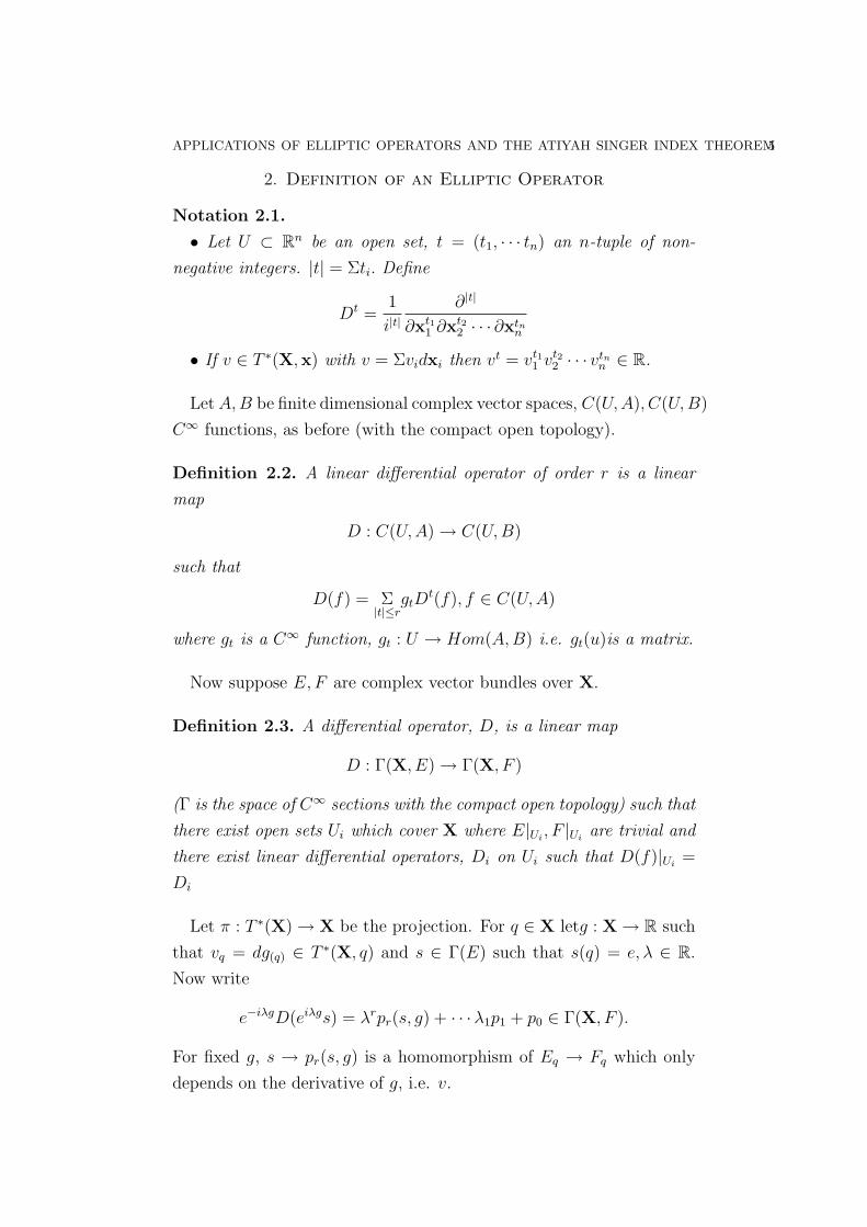
2. Definition of an Elliptic Operator

Notation 2.1.

• Let U ⊂ Rn be an open set, t = (t1, · · · tn) an n-tuple of non-

negative integers. |t| = Σti. Define

Dt =1

i|t|∂|t|

∂xt11 ∂xt2

2 · · · ∂xtnn

• If v ∈ T ∗(X,x) with v = Σvidxi then vt = vt11 vt2

2 · · · vtnn ∈ R.

Let A, B be finite dimensional complex vector spaces, C(U,A), C(U,B)

C∞ functions, as before (with the compact open topology).

Definition 2.2. A linear differential operator of order r is a linear

map

D : C(U,A) → C(U,B)

such that

D(f) = Σ|t|≤r

gtDt(f), f ∈ C(U,A)

where gt is a C∞ function, gt : U → Hom(A,B) i.e. gt(u)is a matrix.

Now suppose E, F are complex vector bundles over X.

Definition 2.3. A differential operator, D, is a linear map

D : Γ(X, E) → Γ(X, F )

(Γ is the space of C∞ sections with the compact open topology) such that

there exist open sets Ui which cover X where E|Ui, F |Ui

are trivial and

there exist linear differential operators, Di on Ui such that D(f)|Ui=

Di

Let π : T ∗(X) → X be the projection. For q ∈ X letg : X → R such

that vq = dg(q) ∈ T ∗(X, q) and s ∈ Γ(E) such that s(q) = e, λ ∈ R.

Now write

e−iλgD(eiλgs) = λrpr(s, g) + · · ·λ1p1 + p0 ∈ Γ(X, F ).

For fixed g, s → pr(s, g) is a homomorphism of Eq → Fq which only

depends on the derivative of g, i.e. v.

6 MARTIN BENDERSKY

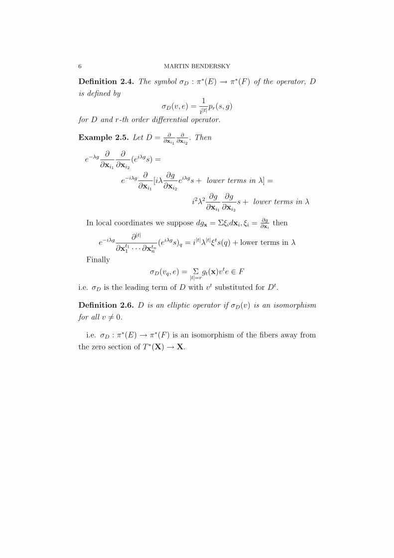
Definition 2.4. The symbol σD : π∗(E) → π∗(F ) of the operator, D

is defined by

σD(v, e) =1

i|t|pr(s, g)

for D and r-th order differential operator.

Example 2.5. Let D = ∂∂xi1

∂∂xi2

. Then

e−λg ∂

∂xi1

∂

∂xi2

(eiλgs) =

e−iλg ∂

∂xi1

[iλ∂g

∂xi2

eiλgs + lower terms in λ] =

i2λ2 ∂g

∂xi1

∂g

∂xi2

s + lower terms in λ

In local coordinates we suppose dgx = Σξidxi, ξi = ∂g∂xi

then

e−iλg ∂|t|

∂xt11 · · · ∂xtn

n

(eiλgs)q = i|t|λ|t|ξts(q) + lower terms in λ

Finally

σD(vq, e) = Σ|t|=r

gt(x)vte ∈ F

i.e. σD is the leading term of D with vt substituted for Dt.

Definition 2.6. D is an elliptic operator if σD(v) is an isomorphism

for all v 6= 0.

i.e. σD : π∗(E) → π∗(F ) is an isomorphism of the fibers away from

the zero section of T ∗(X) → X.


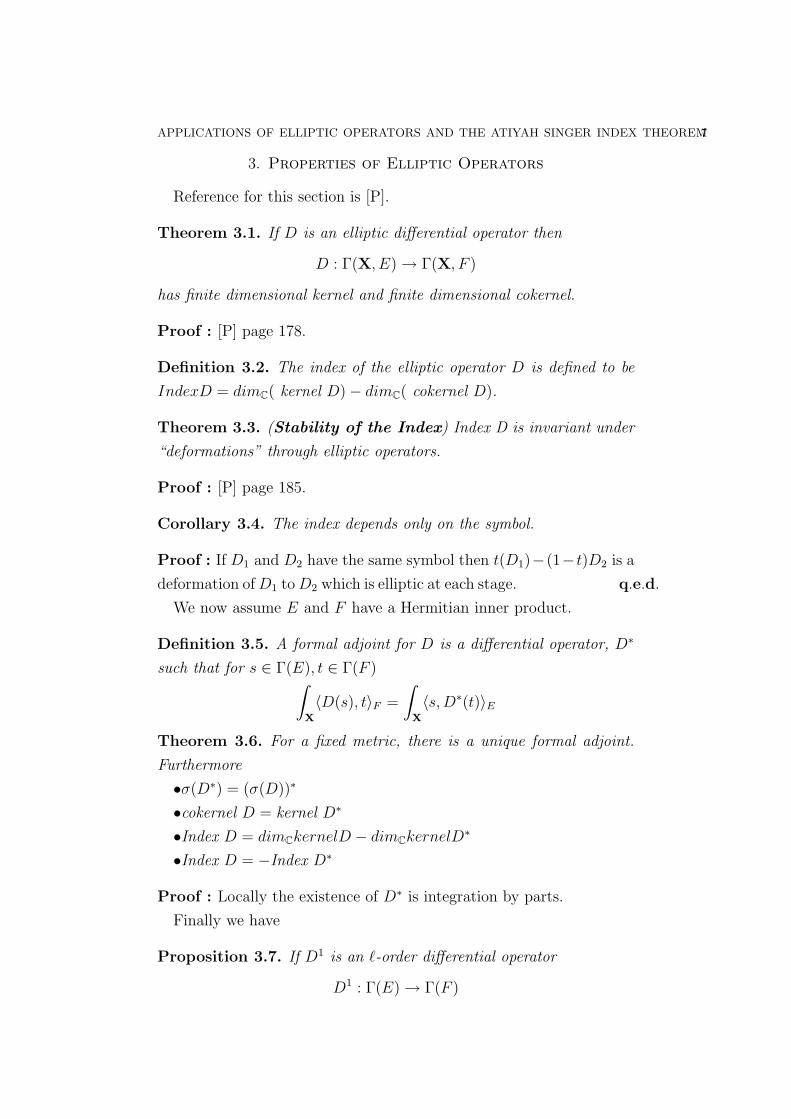
3. Properties of Elliptic Operators

Reference for this section is [P].

Theorem 3.1. If D is an elliptic differential operator then

D : Γ(X, E) → Γ(X, F )

has finite dimensional kernel and finite dimensional cokernel.

Proof : [P] page 178.

Definition 3.2. The index of the elliptic operator D is defined to be

IndexD = dimC( kernel D)− dimC( cokernel D).

Theorem 3.3. (Stability of the Index) Index D is invariant under

“deformations” through elliptic operators.

Proof : [P] page 185.

Corollary 3.4. The index depends only on the symbol.

Proof : If D1 and D2 have the same symbol then t(D1)− (1− t)D2 is a

deformation of D1 to D2 which is elliptic at each stage. q.e.d.

We now assume E and F have a Hermitian inner product.

Definition 3.5. A formal adjoint for D is a differential operator, D∗

such that for s ∈ Γ(E), t ∈ Γ(F )∫

X

〈D(s), t〉F =

∫

X

〈s,D∗(t)〉E

Theorem 3.6. For a fixed metric, there is a unique formal adjoint.

Furthermore

•σ(D∗) = (σ(D))∗

•cokernel D = kernel D∗

•Index D = dimCkernelD − dimCkernelD∗

•Index D = −Index D∗

Proof : Locally the existence of D∗ is integration by parts.

Finally we have

Proposition 3.7. If D1 is an `-order differential operator

D1 : Γ(E) → Γ(F )

8 MARTIN BENDERSKY

and D2 is a k-th order differential operator

D2 : Γ(F ) → Γ(G)

then

σk+` = σ`(D2)σk(D

1)


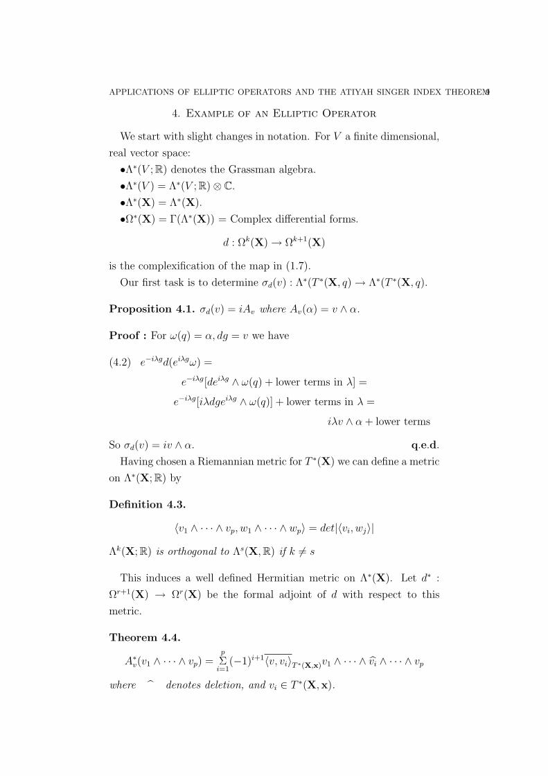
4. Example of an Elliptic Operator

We start with slight changes in notation. For V a finite dimensional,

real vector space:

•Λ∗(V ;R) denotes the Grassman algebra.

•Λ∗(V ) = Λ∗(V ;R)⊗ C.

•Λ∗(X) = Λ∗(X).

•Ω∗(X) = Γ(Λ∗(X)) = Complex differential forms.

d : Ωk(X) → Ωk+1(X)

is the complexification of the map in (1.7).

Our first task is to determine σd(v) : Λ∗(T ∗(X, q) → Λ∗(T ∗(X, q).

Proposition 4.1. σd(v) = iAv where Av(α) = v ∧ α.

Proof : For ω(q) = α, dg = v we have

(4.2) e−iλgd(eiλgω) =

e−iλg[deiλg ∧ ω(q) + lower terms in λ] =

e−iλg[iλdgeiλg ∧ ω(q)] + lower terms in λ =

iλv ∧ α + lower terms

So σd(v) = iv ∧ α. q.e.d.

Having chosen a Riemannian metric for T ∗(X) we can define a metric

on Λ∗(X;R) by

Definition 4.3.

〈v1 ∧ · · · ∧ vp, w1 ∧ · · · ∧ wp〉 = det|〈vi, wj〉|Λk(X;R) is orthogonal to Λs(X,R) if k 6= s

This induces a well defined Hermitian metric on Λ∗(X). Let d∗ :

Ωr+1(X) → Ωr(X) be the formal adjoint of d with respect to this

metric.

Theorem 4.4.

A∗v(v1 ∧ · · · ∧ vp) =

p

Σi=1

(−1)i+1〈v, vi〉T ∗(X,x)v1 ∧ · · · ∧ vi ∧ · · · ∧ vp

where denotes deletion, and vi ∈ T ∗(X,x).

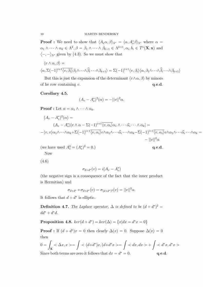
10 MARTIN BENDERSKY

Proof : We need to show that 〈Avα, β〉Λ∗ = 〈α, A∗vβ〉Λ∗ where α =

α1 ∧ · · · ∧ αk ∈ Λk, β = β1 ∧ · · · ∧ βk+1 ∈ Λk+1, αi, bi ∈ T ∗(X,x) and

〈−,−〉Λ∗ given by (4.3). So we must show that

〈v ∧ α, β〉 =

〈α, Σ(−1)i+1〈v, βi〉β1∧· · ·∧βi · · ·∧βk+1〉 = Σ(−1)i+1〈v, βi〉〈α, β1∧· · ·∧βi · · ·∧βk+1〉But this is just the expansion of the determinant 〈v∧α, β〉 by minors

of he row containing v. q.e.d.

Corollary 4.5.

(Av − A∗v)

2(α) = −||v||2α.

Proof : Let α = α1 ∧ · · · ∧ αk.

(Av − A∗v)

2(α) =

(Av − A∗v)[v ∧ α− Σ(−1)i+1〈v, αi〉α1 ∧ · · · αi · · · ∧ αk] =

−〈v, v〉α1∧· · ·∧αk+Σ(−1)i+1〈v, αi〉v∧α1∧· · · αi · · ·∧αk−Σ(−1)i+1〈v, αi〉v∧α1∧· · · αi · · ·∧αk =

− ||v||2α(we have used A2

v = (A∗v)

2 = 0.) q.e.d.

Now

(4.6)

σd+d∗(v) = i(Av − A∗v)

(the negative sign is a consequence of the fact that the inner product

is Hermitian) and

σd+d∗ σd+d∗(v) = σ(d+d∗)2(v) = ||v||2α.

It follows that d + d∗ is elliptic.

Definition 4.7. The Laplace operator, ∆ is defined to be (d + d∗)2 =

dd∗ + d∗d.

Proposition 4.8. ker(d + d∗) = ker(∆) = x|dx = d∗x = 0

Proof : If (d + d∗)x = 0 then clearly ∆(x) = 0. Suppose ∆(x) = 0

then

0 =

∫

X

< ∆x, x >=

∫< (d+d∗)x, (d+d∗x >=

∫< dx, dx > +

∫< d∗x, d∗x >

Since both terms are zero it follows that dx = d∗ = 0. q.e.d.


Definition 4.9. ker ∆ = the Harmonic forms.

Using the sequence

→ Ωi d−→ Ωi+1 →we define

Definition 4.10. Hn(X;C) = ker d/image d.

By proposition (4.8) a Harmonic form represents an element of H∗(X,C).

We say α ∈ H∗(X;C) has a harmonic representative if ∃a ∈ ker∆ such

that [a] = α.

Theorem 4.11. (Hodge Theorem) Every class in H∗(X;C) has a

unique harmonic representative. i.e. ker∆ = H∗(X;C).

12 MARTIN BENDERSKY

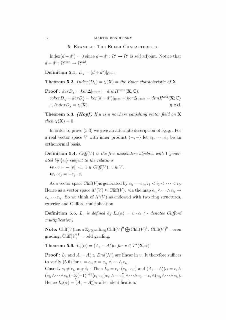
5. Example: The Euler Characteristic

Index(d + d∗) = 0 since d + d∗ : Ω∗ → Ω∗ is self adjoint. Notice that

d + d∗ : Ωeven → Ωodd.

Definition 5.1. Dχ = (d + d∗)|Ωeven

Theorem 5.2. Index(Dχ) = χ(X) = the Euler characteristic of X.

Proof : kerDχ = ker∆|Ωeven = dimHeven(X,C).

cokerDχ = kerD∗χ = ker(d + d∗)|Ωodd = ker∆|Ωodd = dimHodd(X;C)

∴ IndexDχ = χ(X). q.e.d.

Theorem 5.3. (Hopf) If u is a nowhere vanishing vector field on X

then χ(X) = 0.

In order to prove (5.3) we give an alternate description of σd+d∗ . For

a real vector space V with inner product 〈−,−〉 let e1, · · · , ek be an

orthonormal basis.

Definition 5.4. Cliff(V ) is the free associative algebra, with 1 gener-

ated by ei subject to the relations

•v · v = −||v|| · 1, 1 ∈ Cliff(V ), v ∈ V .

•ei · ej = −ej · ei

As a vector space Cliff(V )is generated by ei1 · · · ei` , i1 < i2 < · · · < i`.

Hence as a vector space Λ∗(V ) ≈ Cliff(V ). via the map ei1 ∧· · ·∧ei` 7→ei1 · · · ei` . So we think of Λ∗(V ) as endowed with two ring structures,

exterior and Clifford multiplication.

Definition 5.5. Lv is defined by Lv(α) = v · α ( · denotes Clifford

multiplication).

Note: Cliff(V )has a Z2-grading Cliff(V )0 ⊕Cliff(V )1. Cliff(V )0 =even

grading, Cliff(V )1 = odd grading.

Theorem 5.6. Lv(α) = (Av − A∗v)α for v ∈ T ∗(X,x)

Proof : Lv and Av−A∗v ∈ End(Λ∗) are linear in v. It therefore suffices

to verify (5.6) for v = ei, α = ei1 ∧ · · · ∧ eit .

Case I. ei 6= ei` any i`.. Then Lv = ei · (ei1 · eit) and (Av−A∗v)α = ei∧

(ei1∧· · ·∧eit)−Σr(−1)r+1〈ei, eir〉ei1∧· · · eir∧· · ·∧eit = ei∧(ei1∧· · ·∧eit).

Hence Lv(α) = (Av − A∗v)α after identification.


Case II. ei = eir for some ir. then Lv(α) = (−1)rei1 · · · eir · · · ei` .

(Av−A∗v)(α) = eir ∧ ei1 ∧ · · · ∧ ei`︸︷︷︸

=0

−Σ(−1)t+1〈eir , eit〉ei1∧· · · eit∧· · ·∧ei` = Lv(α).

Corollary 5.7. σd+d∗ = iLv

Proof : This follows from (5.6) and (4.6). q.e.d.

Notice that (4.5) follows from the Clifford identities.

Now continuing with the proof of (5.3). We identify T (X,R) with

T ∗(X,R) via the metric. The vector field, u determines a non-vanishing

1-form, which we also denote by u. Define Bu : Ω∗(X) → Ω∗(X) by

Bu(α) = a∧u. B∗u is the adjoint and, as in (5.6) Ru = Bu−B∗

u is right

Clifford multiplication. R2u = −||u||2id. Furthermore Ru sends Ωodd

to Ωeven and visa versa. So we have a diagram:

(5.8)

Ωeven Dx−→ ΩoddyRu

yRu

Ωodd Dx−→ Ωeven

We claim that (5.8) commutes on the symbol level.

Proof : On the level of symbols, using (3.7), and thinking of Ru as a

zero order operator we have

σRuDx(ν) = (να)u, σD∗Ru(ν) = ν(αu).

The claim now follows for the associative law in Cliff(V).

Hence by (3.4)

Index (Ru Dx) = Index (D∗x Ru)

But Ru is an isomorphism (since u 6= 0). So

Index (Ru Dx) = Index (Dx)

Index (D∗x Ru) = Index (D∗

x)

Hence by (3.6) Index (Dx) = χ(X) = 0.

14 MARTIN BENDERSKY

6. Example: The Signature Invariant

Let V be a finite dimensional, real vector space. 〈−,−〉 a symmetric,

non-degenerate , bilinear form on V . There is a basis e1, · · · , em, f1, · · · , fnof V such that 〈ei, ej〉 = δ − i, j, 〈fi, fj〉 = −δi,j, 〈ei, fj〉 = 0.

Definition 6.1. The signature of 〈−,−〉 is defined to be m− n.

Now let X be a closed oriented manifold of dimension n = 4k. Then

on the real vector space H2k(X;R) we have the bilinear form 〈α, β〉 =

α ∪ β[X]. This form is symmetric (because n = 4k) and non-singular

(because of Poincare’ duality).

Definition 6.2. Sign(X) = signature(〈−,−〉).

We now look for a differential operator whose index is Sign(X).

Let ω ∈ Λn(X) be a volume form, i.e. ωx = e1 ∧ · · · ∧ en where

e1, · · · en is any orthonormal basis for T ∗(X,x).

An operator ∗ : Λp(X,R) → Λn−p(X,R) is defined by the formula

(6.3) [λ ∧ (∗µ)]n = 〈λ, µ〉Λ∗Rωx

for λ, µ ∈ Λ∗x and for t ∈ Λ∗, [t]n denotes the term with grading n.

By linearity there is induced

∗ : Λp(X) → Λn−p(X)

and

∗; Ωp(X) → Ωn−p(X)

Locally, if e1, · · · , en is a basis of T ∗(X,x) (with the same orientation

as e1, · · · en) then

(6.4) ∗(e1 ∧ · · · ∧ ep) = ep+1 ∧ · · · ∧ en


Properties of ∗ : Ω∗ → Ω∗

Since ∗ is the complexification of a real operator we have

(6.5) ∗(β) = ∗β.

Such an operator is called a real operator.

Note: If V is a complex vector space with a conjugation, v, we define

VR to be the fixed space of conjugation and we have

(6.6) V = VR ⊗ C.

If L : V → W is an operator which commutes with conjugation (i.e. a

real operator) then L induces LR : VR → WR and L = LR ⊗ C.

Proposition 6.7. If α ∈ Λi then ∗ ∗ α = (−1)iα

Proof : Let α = e1 ∧ · · · ei then ∗α = ei+1 ∧ · · · ∧ en

(6.8) (λ ∧ (∗ ∗ α)) = 〈λ, ∗α〉ωx

Let λ = ei+1 ∧ · · · ∧ en. Then ∗ ∗ α = εe1 ∧ · · · ∧ ei. From (6.8) we

have

ε(ei+1 ∧ · · · ∧ en ∧ e1 ∧ · · · ∧ ei) = e1 ∧ · · · ∧ en

Hence ε = (−1)i(n−i) = (−1)i q.e.d.

We also have, from (6.3)

(6.9)

∫

X

〈α, β〉Λ∗ =

∫

X

(α ∧ ∗β)n

In fact the notation∫X〈α, β〉 stands for the integral

∫X〈α, β〉ω.

Proposition 6.10.

d∗ = − ∗ d∗

Proof : Let f ∈ Ωp, g ∈ Ωp+1. We must show that∫

X

〈df, g〉 =

∫

X

〈f,− ∗ d∗〉

Now d(f ∧ (∗g))n = (df ∧ (∗g))n + (−1)p(f ∧ d(∗g))n, so we have

(6.11)

∫

X

d(f ∧ (∗g))n =

∫

X

(df ∧ (∗g))n + (−1)p

∫

X

(f ∧ d ∗ g))n.

16 MARTIN BENDERSKY

But X has no boundary, so by Stoke’s theorem the left hand side of

(6.11) is zero. Using (6.7) and (6.9) we obtain

0 =

∫

X

〈df, g〉+ (−1)p(−1)n−p

∫

X

〈f, ∗d ∗ g〉

and (6.10) follows. q.e.d.

Recall the dimension of X is n = 4k. Let α ∈ Ωp

Definition 6.12. τ(α) = (−1)p(p−1)

2+k ∗ (α)

By (6.7) τ 2(α) = α.

On each fiber we have the eigenspaces Λx+ , Λx− of τx. We therefore

have a decomposition Λx = Λx+

⊕Λx− . Because τ : Λ∗ → Λ∗ is equi-

variant under the action of SO(n), we may glue Λx+and Λx− together to

obtain subbundles Λ+(X) and Λ−(X) such that Λ∗ = Λ∗+(X)⊕

Λ∗−(X).

Correspondingly we get a decomposition Ω∗ = Ω∗+

⊕Ω∗− and Ω∗(X,R) =

Ω∗+(X,R)

⊕Ω∗−(X,R). So if ϕ ∈ Ω∗

±, τ(ϕ) = ±ϕ.

Proposition 6.13.

τ(d + d∗) = −(d + d∗)τ

Proof : Use ∗2 = (−1)k on Ωk, d∗ = − ∗ d∗ and the definition of τ

q.e.d.

So d + d∗ defines a homomorphism

DS : Ω+ → Ω−

The formal adjoint of DS, D∗S : Ω− → Ω+ is the restriction of d+ d∗.

Theorem 6.14. Index (DS) = Signature(X)

Proof : Let ∆ = (d + d∗)2, τ∆ = ∆τ . Identify ker ∆ (=harmonic

forms)with H∗(X;C). We have τ : H∗(X;C) → H∗(X;C) such that

τ 2 = id and a decomposition

H∗(X;C) = H∗+(X;C)

⊕H∗−(X;C).

So Index (DS) = dim H∗+(X;C) − dim H∗

−(X;C). We first look at

H`(X;C)⊕

Hn−`(X;C), ` < 2k. Then τ leaves this invariant. Let

H`± =

= x ∈ H`(X;C)

⊕Hn−`(X;C)|τ(x) = ±x ` < 2k,

H2k± ` = 2k


Then

(6.15) H∗±(X,C) =

⊕

`≤2k

H`±

(To see this let y ∈ H∗±(X,C) be y = y0 + y1 + · · · yn, yi ∈ H i. Then

apply τ to Σyi and use the definition of H∗±.) The argument in the

parenthesis shows that for ` < 2k, H`± = x ± τ(x), x ∈ H`(X;C).

Using (6.15) we see that the map x 7→ x± τ(x) gives an isomorphism

H`(X;C) → H`±(X;C), ` < 2k.

So Index (DS) = dim H2k+ − dim H2k

−On H2k(X;C) τ = ∗ (because (−1)

2k(2k−1)2

+k = 1). Since τ is a real

operator we have

H2k± (X;C) = H2k

± (X;R)⊗ C

(see (6.5)) and Index (DS) = Real dim H2k+ (X;R)−Real dim H2k

− (X;R).

By the DeRham theorem the form a ∪ b is given by∫X

α ∧ β on

H2k(X;R). Now let α ∈ H2k+ . Then

α ∪ α =

∫α ∧ α =

∫α ∧ τ(a) =

∫α ∧ ∗α =

∫〈α, α〉 > 0

If β ∈ H2k− then

β ∪ β =

∫β ∧ β = β ∧ −τ(β) = −

∫β ∧ ∗β < o

We also have

α ∪ β =

∫α ∧ β =

∫α ∧ −τ(β) = −

∫a ∧ ∗β = −

∫〈α, β〉Λ∗

β ∪ α =

∫β ∧ α =

∫β ∧ τ(α) =

∫β ∧ ∗α =

∫〈β, α〉Λ∗

But on H2k 〈α, β〉Λ∗ = 〈β, α〉Λ∗ , α ∪ β = β ∪ α. So H2k+ ⊥H2k

− .

q.e.d.

18 MARTIN BENDERSKY

7. A Theorem of Atiyah, Frank and Mayer

Recall the definition of Cliff(V ) (see 5.4). For V = Rn, 〈−,−〉 =

the usual inner product, we denote Cliff(Rn) by Cn.

Let M be a real vector space which is a Cliff(V)n module. We

say M is a Z2 graded Cliff(V)n module if M = M0⊕

M1 and

Cliff(V)in · M j ⊂ M i+j, (i, j ∈ Z2). The following result requires

a deeper knowledge of the structure of Cliff(V)n and will be proven

in §8.

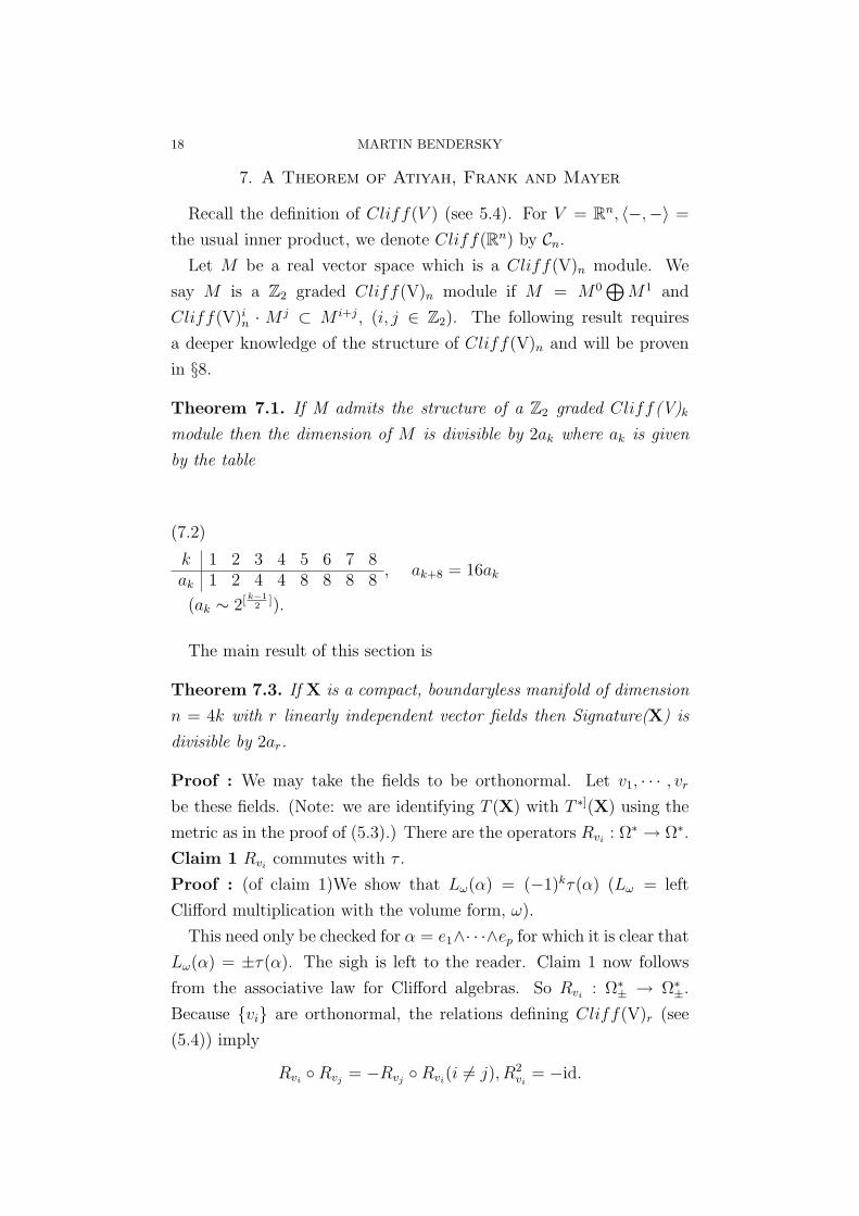
Theorem 7.1. If M admits the structure of a Z2 graded Cliff(V)k

module then the dimension of M is divisible by 2ak where ak is given

by the table

(7.2)

k 1 2 3 4 5 6 7 8ak 1 2 4 4 8 8 8 8

, ak+8 = 16ak

(ak ∼ 2[ k−12

]).

The main result of this section is

Theorem 7.3. If X is a compact, boundaryless manifold of dimension

n = 4k with r linearly independent vector fields then Signature(X) is

divisible by 2ar.

Proof : We may take the fields to be orthonormal. Let v1, · · · , vr

be these fields. (Note: we are identifying T (X) with T ∗](X) using the

metric as in the proof of (5.3).) There are the operators Rvi: Ω∗ → Ω∗.

Claim 1 Rvicommutes with τ .

Proof : (of claim 1)We show that Lω(α) = (−1)kτ(α) (Lω = left

Clifford multiplication with the volume form, ω).

This need only be checked for α = e1∧· · ·∧ep for which it is clear that

Lω(α) = ±τ(α). The sigh is left to the reader. Claim 1 now follows

from the associative law for Clifford algebras. So Rvi: Ω∗

± → Ω∗±.

Because vi are orthonormal, the relations defining Cliff(V)r (see

(5.4)) imply

RviRvj

= −RvjRvi

(i 6= j), R2vi

= −id.


It was shown (c.f. (5.8)) that σd+d∗ commutes with Rvi. Let G be the

group generated by Rvi. The relations among the Rvi

’s imply G is

finite. Define the operator

T =1

|G| Σg∈G

g(d + d∗)g−1

Since Rvi∈ G, T commutes with G. Also since σd+d∗ and Rvi

com-

mute σT = σd+d∗ . Therefore by the stability of elliptic operators (3.4)

Index(T )=Index(DS). But for T , kerT : Ω+ → Ω− is a module

over G = Cr. Furthermore Ω+ = Ωeven+

⊕Ωodd− gives a Z2 grad-

ing to ker(T ). Similar comments apply to coker(T ) = kerΩ− →Ω+. Therefore by (7.2) ker(T ) − coker(T ) = Index T = Index Ds =

Signature(X) is divisible by 2ar. q.e.d.

20 MARTIN BENDERSKY

8. Clifford Algebras

The reference for this section is [ABS]. Let V be a vector space with

orthonormal basis e1, · · · ek. Recall the definition of Ck.

(8.1)

Ck is the free associative algebra generated byei subject to therelations

eiej + ejei = 0, i 6= j, e2i = −1

Definition 8.2. C ′k is the free associative algebra generated by eisubject to the relations eiej + ejei = 0, i 6= j, e2

i = 1

C ′k is introduced in order to calculate Ck. There are isomorphisms:

(8.3)

u : Ck+2 → C ′k ⊗ C2 v : C ′k+2 → Ck ⊗ C ′2

(8.4)

Ck ⊗ C ≈ C ′k ⊗ C

(8.5)

Ck+4 ≈ Ck ⊗ C4 C ′k+4 ≈ C ′k ⊗ C ′4

(8.6)

Ck+8 ≈ Ck ⊗ R(16)

(We use the notation F (n) for the algebra of n × n matrices over F ,

F = R,C, or H1 There are relations F ⊗ R(n) = F (n), and F ⊗(R

⊕R) = F

⊕F .) All tensors in the following are over R.

Proof : of (8.3). Let e1, · · · , ek be algebra generators for Ck and

e′1, · · · , e′k algebra generators of C ′k. Define u : Rk+2 → C ′k ⊗ C2 by

u(e1) = 1⊗ e1, u(e2) = 1⊗ e2, u(ei) = e′i−2 ⊗ e1e2 if 3 ≤ i ≤ k + 2.

The u takes the defining relations to zero and passes a homomorphism

1H is generated by elements 1, i, j, k such that i2 = j2 = k2 = −1, and

ij = −ji = k, jk = −kj = i, ki = −ik = j.

If a = a0 + a1i + a2j + a3k, a = a0 − a1i− a2j − a3k


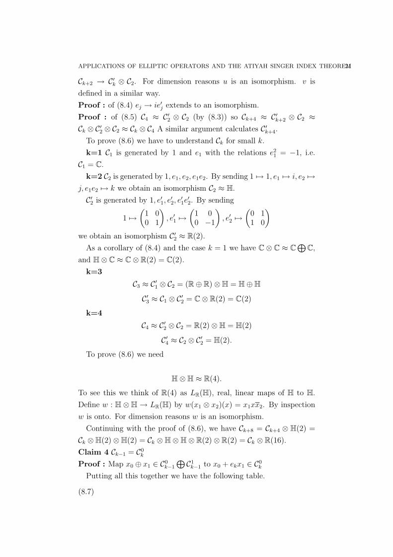
Ck+2 → C ′k ⊗ C2. For dimension reasons u is an isomorphism. v is

defined in a similar way.

Proof : of (8.4) ej → ie′j extends to an isomorphism.

Proof : of (8.5) C4 ≈ C ′2 ⊗ C2 (by (8.3)) so Ck+4 ≈ C ′k+2 ⊗ C2 ≈Ck ⊗ C ′2 ⊗ C2 ≈ Ck ⊗ C4 A similar argument calculates C ′k+4.

To prove (8.6) we have to understand Ck for small k.

k=1 C1 is generated by 1 and e1 with the relations e21 = −1, i.e.

C1 = C.

k=2 C2 is generated by 1, e1, e2, e1e2. By sending 1 7→ 1, e1 7→ i, e2 7→j, e1e2 7→ k we obtain an isomorphism C2 ≈ H.

C ′2 is generated by 1, e′1, e′2, e

′1e′2. By sending

1 7→(

1 00 1

), e′1 7→

(1 00 −1

), e′2 7→

(0 11 0

)

we obtain an isomorphism C ′2 ≈ R(2).

As a corollary of (8.4) and the case k = 1 we have C⊗ C ≈ C⊕C,

and H⊗ C ≈ C⊗ R(2) = C(2).

k=3

C3 ≈ C ′1 ⊗ C2 = (R⊕ R)⊗H = H⊕HC ′3 ≈ C1 ⊗ C ′2 = C⊗ R(2) = C(2)

k=4

C4 ≈ C ′2 ⊗ C2 = R(2)⊗H = H(2)

C ′4 ≈ C2 ⊗ C ′2 = H(2).

To prove (8.6) we need

H⊗H ≈ R(4).

To see this we think of R(4) as LR(H), real, linear maps of H to H.

Define w : H ⊗ H → LR(H) by w(x1 ⊗ x2)(x) = x1xx2. By inspection

w is onto. For dimension reasons w is an isomorphism.

Continuing with the proof of (8.6), we have Ck+8 = Ck+4 ⊗ H(2) =

Ck ⊗H(2)⊗H(2) = Ck ⊗H⊗H⊗ R(2)⊗ R(2) = Ck ⊗ R(16).

Claim 4 Ck−1 = C0k

Proof : Map x0 ⊕ x1 ∈ C0k−1

⊕ C1k−1 to x0 + ekx1 ∈ C0

k

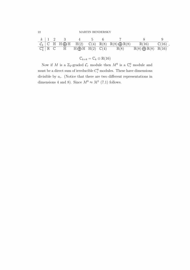
Putting all this together we have the following table.

(8.7)

22 MARTIN BENDERSKY

k 1 2 3 4 5 6 7 8 9Ck C H H

⊕H H(2) C(4) R(8) R(8)

⊕R(8) R(16) C(16)

C0k R C H H

⊕H H(2) C(4) R(8) R(8)

⊕R(8) R(16)

,

Ck+8 = Ck ⊗ R(16)

Now if M is a Z2-graded Cr module then M0 is a C0r module and

must be a direct sum of irreducible C0r modules. These have dimensions

divisible by ar. (Notice that there are two different representations in

dimensions 4 and 8). Since M0 ≈ M1 (7.1) follows.


9. A Diversion: Constructing Vector Fields on Spheres

using Clifford Algebras

In this section we show how Clifford algebras may be used to con-

struct vector fields on spheres. We will make no use of previous sections,

nor will it be used in subsequent sections. We simply include it for the

readers amusement.

Write n as odd 24d+c, 0 ≤ c < 4.

Definition 9.1. The Hurwicz-Radon number, ρ(n) is defined by ρ(n) =

2c + 8d

It may be seen from table (7.2) that Rn is a Cρ(n)−1 module. i.e. there

is an action Rn × Cρ(n)−1−→ Rn and ρ(n) is the largest such number.

Theorem 9.2. There are ρ(n)−1 linearly independent vector fields on

Sn−1

It is wonderful theorem of Frank Adams that there are not ρ(n)

independent vector fields on Sn−1.

Proof : We define a map

µ : Rρ(n) × Rn → Rn

by

(ei, r) 7→ ei · r, 1 ≤ i < ρ(n)

(eρ(n), r) 7→ r

For 1 ≤ i ≤ ρ(n) let ui : Rn → Rn be defined by ui(r) = µ(ei, r). In

particular uρ(n) = the identity.

Notice we have an inner product on Rρ(n) which was used to define

Cρ(n)−1. We have not yet specified the inner product on Rn. Let U be

the group generated by ui ∈ GL(n). By the Clifford identities U is

finite (in fact it has 2n elements). For 〈−,−〉′ and metric on Rn we

define

〈x, y〉n =1

|U| Σu∈U〈u(x), u(y)〉′

with respect to this metric ui ∈ O(n). For future reference we list

the identities among the ui which follow from the Clifford relations for

24 MARTIN BENDERSKY

i < ρ(n):

u2i = −id , uiuj + ujui = 0, if i 6= j.

We shall show that the above relations will imply a relation among

the two norms. Specifically for x ∈ Sn−1

(9.3)

||µ(y, x)||n = ||y||ρ(n).

From this it will follow that for x ∈ Sn−1, y1, y2 ∈ Rρ(n) we have

〈µ(y1, x), µ(y2, x)〉Rn = 〈y1, y2〉Rρ(n)

Proof : We write || − ||Rk as || − ||k

(9.4) 〈µ(y1, x), µ(y2, x)〉n =

1

2(||µ(y1, x) + µ(y2, x)||n − ||µ(y1, x)||n − ||µ(y2, x)||n) =

1

2(||y1 + y2||ρ(n) − ||y)1||ρ(n) − ||y2||ρ(n)) = 〈y1, y2〉ρ(n)

From (9.4) it follows that ui(x)i=1,···ρ(n) are mutually orthonormal.

for x ∈ Sn−1. Since uρ(n) = the identity we have proven (9.2) once we

have proven (9.3).

Proof of (9.3). It suffices to show that ||µ(u, x)||n = 1 for x ∈Sn−1, ||y||ρ(n) = 1. This is equivalent to proving that µ(y,−) ∈ O(n)

for any ||y||ρ(n) = 1. i.e. we must show that

µ(ρ(n)

Σi=1

aiei, x) =ρ(n)

Σi=1

aiui(x) = 1

forρ(n)

Σi=1

a2i = 1, x ∈ Sn−1. So we have to prove that v = Σaiui ∈ O(n)

for Σa2i = 1. We recall that a linear transformation, ω, belongs to O(n)

⇔ ωω∗ = 1 where ω∗ is the adjoint. In particular ω∗ = ω−1. For ω = ui

we have u∗ = u−1i = −ui. Now

(9.5) ωω∗ = (Σaiui)(Σ(aiu∗i ) = Σa2

i uiu∗i + Σ

i<jaiaj(uiu

∗j + uju

∗i )

Because Σa2i = 1 the first summation is 1. For j = ρ(n) in the second

summand uj = u∗j = the identity and uiu∗ρ(n) + uρ(n)u

∗i = ui − ui = 0

for i < ρ(n).


For j < ρ(n)

uiu∗j + uju

∗i = −(uiuj + ujui) = 0.

So ωω∗ = 1 proving (9.2). q.e.d.

26 MARTIN BENDERSKY

10. Topological Invariants of the Index. The Atiyah

Singer Index Theorem

To discuss the topological part of the index theorem it is best to

work in K-theory. For the purpose of these notes we only need the

cohomology calculation of the index. Because of this we shall only

outline the required K-theory. We also outline the needed facts about

ordinary cohomology and Chern classes. Further references are: [A],

[H].

Notation 10.1. A complex vector bundle will be denoted by Greek

letters, ξ, η etc. V ectn(X) = n− dimensional vector bundles over Xup to equivalence. Vect(X) =

⊕n

V ectn(X).

Note: If X is not connected we allow different dimensions for the

bundles over the various path components.

V ect(X) is a semi group under Whitney sum.

For a semi group, G, K(G) denotes the Grothendieck group of G.

i.e. G×G/ ∼ where (α, β) ∼ (α′, β′) if ∃c ∈ G such that α + β′ + c =

α′ + β + c.

Definition 10.2. For X compact K(X) = K(V ect(X))

if f : X → Y is a continuous map then K(f) : K(Y ) → K(X) is

induced by the pullback of bundles.

Each element of K(X) is of the form [ξ]− [η] where [−] denotes the

class of a bundle in the Grothendieck group. K(X) has a ring structure

induced by the tensor product of bundles.

For a point, p, K(p) = Z. If X has a base point, ∗, the map ∗ → X

induces a map K(X)rank−→ Z.

Definition 10.3. K(X) = kernel(rank)

Let V ect(X) be V ect(X)/ ∼ where ξ ∼ η if there are trivial bundles

εa, εb such that ξ ⊕ εa ≈ η ⊕ εb.

(10.4)

K(X) = V ect(X)


where ξ ∈ V ect(X) corresponds to [ξ]− [rank ξ] ∈ K(X).

Note: This identification does not behave well with respect to ⊗.

(10.5)

K(X,A) = K(X/A)

Note: X/∅ =definition

X⋃ disjoint point).

For X locally compact X+ denotes the one point compactification

of X For X compact X+ = X/∅. Then K(X) = K(X+).

(10.6) The clutching construction

Let X = X1

⋃X2, A = X1

⋂X2. We have to assume the triple

(X1, X2, A) is reasonable. Assuming all spaces are C.W. complexes

and subcomplexes will suffice.

Let ηi be a vector bundle over Xi and ϕ : η1|A → η2|A an isomor-

phism.

Definition 10.7. The clutching of η1 with η2 via ϕ , η1

⋃ϕ η2, is defined

as η1

⋃η2/ ∼ where e1 ∈ η1|A ∼ ϕ(e1) ∈ η2|A.

η1

⋃ϕ η2 is a vector bundle over X and η1

⋃ϕ η2|Xi

= ηi, i = 1, 2. See

([H] or [A]) for details.

As an application of the clutching construction we describe the im-

portant difference construction.

Let η1 and η2 be vector bundles over X with ϕ : η1|A → η2|A an

isomorphism. Let Y = X1

⋃A X2 (Xi = X). Then we have an exact

sequence

K(X1)i←− K(Y )

j←− K(Y,X1) ≈ K(X2, A) = K(X, A)

Since there is a folding map making the composite X1i−→ Y

fold−→ X1

the identity if follows that j is an injection (c.f. [A]). There is the

element η1

⋃ϕ η2 − fold(η1) ∈ K(Y ). i(η1

⋃ϕ η2 − fold(η1)) = 0 so

there is a unique element, (η1, ϕ, η2) ∈ K(Y, X1) mapping to η1

⋃ϕ η2−

fold(η1) via j.

28 MARTIN BENDERSKY

Definition 10.8. The difference bundle is defined to be (η1, ϕ, η2) ∈K(Y, X1)

Notice that the map K(X,A) → K(X) sends (η2, ϕ, η1) to [η2]− [η1].

Recall the definition of an elliptic operator, D (2.6). σD : π∗(E) →π∗(F ) is an isomorphism away from the zero section. For any bundle,

η let η0 denote the non-zero vectors. Then the difference element,

(π∗(E), σD, π∗(F ) is an element of K(T ∗(X), T ∗(X)0).

Definition 10.9. We shall denote this class by [σD].

The map K(T ∗(X), T ∗(X)0) → K(T ∗(X)) sends [σD] to [π∗(E)] −[π∗(F )].

For a complex bundle, η, there are the Chern classes, ci(η) (see [MS]).

The total Chern class is defined to be c(η) = 1 + c1(η) + · · ·+ ck(η) (η

is a k plane bundle). We formally factor c(η) as

c(η) =k∏

i=1

(1 + w1) wi is given degree 2

The w′is do not have any meaning, however the elementary symmetric

functions in the w′is do (as the Chern classes). Hence any polynomial

in the elementary symmetric functions in the w′is has meaning. Con-

versely any symmetric polynomial in the w′is is a unique polynomial

in the elementary symmetric functions (see [H]) therefore makes sense.

The important polynomials for us are

(10.10) Ch(η) = Σewi

(10.11) T (η) =∏ wi

1− e−wi

Ch is the Chern character, T is the Todd genus. Notice that Ch and

T lie in H∗∗(X,Q) where H∗∗ =∏

H∗.

Let ηk π−→ B be a real, oriented, k dimensional real bundle over a

compact base B. (We write ηk for the total space as well as for the

bundle.) π∗ : H∗(B) → H∗(η) is an isomorphism. There is a class

U ∈ Hk(η, η0) such that there is a Thom isomorphism map, i.e.

(10.12) ϕ(a) = π∗(a) ∪ U


is an isomorphism (ϕ : H`(B;Q) → H`+k(η, η0;Q))

The Thom isomorphism is true with integral coefficients. Since we

are only interested in rational cohomology it has been stated for coho-

mology with Q coefficients.

Let χ(η) ∈ Hk(B) be the Euler class of η (see [MS]) and ι : H∗(η, η0) →H∗(η) Then the fundamental relationship between χ(η) and the Thom

class is

(10.13) π∗(χ(η)) = ι(U).

Let D be an elliptic operator over X2`.

Definitions

•Ch(D) = (−1)`ϕ−1ch([σD]) (see 10.9).

•T (X) = T (T (X)⊗ C)

Definition 10.14. Indext(D) = 〈Ch(D)T (X), [X]〉

where 〈−,−〉 is the Kronecker pairing and [X] is the fundamental

class.

Theorem 10.15. (Atiyah Singer Index Theorem)

Indext(D) = Index(D).

Note: Indext(D) can be described entirely in terms of K−theory.

While we will not discuss this formulation here, it is quite important.

30 MARTIN BENDERSKY

11. Borel Hirzebruch Theory and Characteristic Classes

A references for much of this material are [MS], [BH].

Let G = SO(2`) orU(`). There is the maximal torus T ` ⊂ G. For

G = U(`), T ` corresponds to the diagonal matrices. For G = SO(2`)

T ` corresponds to matrices with 2× 2 blocks(

x −yy x

), x + iy ∈ S1

on the diagonal. BG and BT denote the classifying spaces.

•BT ` = CP∞ × · · ·CP∞︸︷︷︸

`

•H∗(BT ` ;Q) ∼= Q[x1, · · · x`], xi ∈ H2(BT ` ;Q)

T ` → G induces ρ : H∗(BG;Q) → H∗(BT `Q)

Theorem 11.1. (Borel-Hirzebruch) ρ is an injection. The image is as

follows:

• (a) G = U(`) The image of ρ is the ring of symmetric poly-

nomials over Q. The element ∈ H2i(BG;Q) corresponding to

the i−th elementary symmetric function is the universal Chern

class, ci. 1 + c1 + · · ·+ c` =∏

(1 + xi) via ρ

• (b) G = SO(2`) The image of ρ is the ring of polynomials

symmetric in x2i and the element x1 · · · x`. The element ∈

H4i(BGQ) corresponding to the i − th elementary symmetric

function in the x2i ’s is the universal Pontrijagin class, ℘i. 1 +

℘1 + · · ·℘` =∏

(1 + x2i ). The universal Euler class corresponds

to∏

xi

In the sequel we shall identify H∗(BG;Q) with its image via ρ. A

(complex) G−module is a (complex) vector space, M with an action

of G on M .

Definition 11.2. M = EG ×G M (EG ×G M = EG × M/ ∼, where

(eg, g−1m) ∼ (e,m)).

We wish to understand the characteristic classes of M . For this we

introduce an isomorphism

ν : Hom(T, S1) → H2(BT ;Z)


where T is the torus and S1 = R/Z. We identify S1 with U(1) via

the map s 7→ e2πis, (s ∈ R/Z). Then for f : T → S1 = U(1)we

obtain a map Bf : BT → BU(1) which defines a line bundle, ξf over BT .

ν(f) = c1(ξf ), the first Chern class.

Case 1 Suppose M is a complex vector space of dimension n. By

restriction M is a T module (T ⊂ G). Then M is a direct sum of

irreducible T modules of dimension 1

M = M1

⊕· · ·

⊕Mn

and T acts, for m ∈ Mj by

t ·m = e2πiwj(t)m

for wj ∈ Hom(T, S1). The wi’s are called the weights of M . Using ν

we may think of the wi’s as elements of H2(BT ;Q). We then have the

formula

1 + c1(M) + · · ·+ cn(M) =∏

(1 + wi)

[Here we re identifying H∗(BG) with its image via ρ). So Ch(M) =

Σewi .

The Pontrijagin classes of the underlying real bundle, M ′ are

1 + ℘1(M′) + · · ·+ ℘n(M ′) =

∏(1 + w2

i )

Case 2 Suppose M is a real vector space of dimension 2n. By

restriction M is a T module. Hence M is a direct sum of 2−dimensional

T modules.

(11.3) M = M1

⊕· · ·

⊕Mn

Give M a G invariant metric. Then with respect to an orthonormal

basis of Mj

t ·m =

(cos2πwj(t) −sin2πwj(t)sin2πwj(t) cos2πwj(t)

)m

m ∈ Mj, wj ∈ Hom(T, S1). Again we call wj the weights of M which

now depend on the orientation of Mj. The total Pontrijagin class is

32 MARTIN BENDERSKY

1 + ℘1(M) + · · ·+ ℘n(M) =∏

(1 + w2j )

If M is oriented and (11.3) agrees with the orientations then we have

for the Euler class

χ(M) =∏

(wi).

The weights of M ⊗ C as a complex bundle are ±w1, · · · ,±wn and

1 + c1(M ⊗ C) + · · ·+ cn(M ⊗ C) =∏

(1 + wi)(1−wi) =∏

(1−w2i ).

So we have the formula

℘i(M) = (−1)ic2i(M ⊗ C)

which in [MS] is taken as the definition of the ℘i’s.

As a consequence if ℘(T (X)) =∏

(1 + y2i ) then

(11.4) T (X) = T (T (X)⊗ C) =∏

(yi

1− e−yi)(

−yi

1− eyi).

With these preliminaries behind us we are now ready to calculate

indext(D). The secret is to pass to the universal case. For this we

assume the Riemannian structure on X2` is specified as follows:

• There is an fixed oriented, real SO(2`) module ,V.

• We have a principle SO(2`) bundle. P over X.

• There is an orientation preserving isomorphisms χ : P ×G V ∼=T (X).


12. Verification of the Index Theorem for Dχ

Convention 12.1. The methods of this and the following sections ap-

ply to bundles, η → X which are of the form P×GM for some G-module

M (G = SO(2`)), P a principle G bundle over X.

For example:

• Λ∗(X) = P ×G Λ∗(V )

• Λ∗±(X) = P ×G Λ∗±(V )

Let f : X → BG classify P → X. Then T (X) = f ∗(V ) (see (11.2)

for definition of V ). Recall the diagram involving the symbol σD

(12.2)

π∗(E)σD−→ π∗(F ) E F

T ∗(X)

π−→ X

This gave us an element [σD] ∈ K(T ∗(X), T ∗(X)0),(10.9).

Let E and F be SO(2`) modules defining E and F as described in

(12.1). E, F the vector bundles over BG (as in (11.2)).

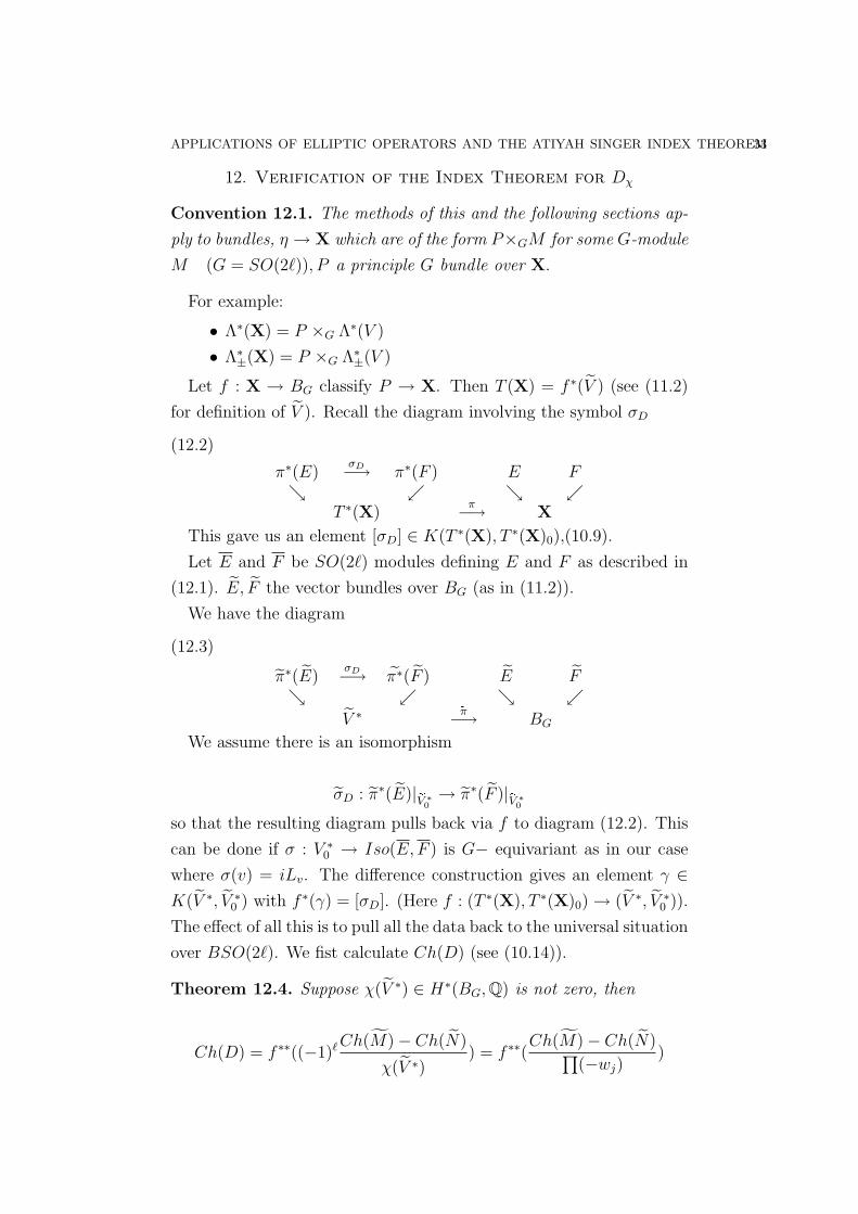
We have the diagram

(12.3)

π∗(E)σD−→ π∗(F ) E F

V ∗ eπ−→ BG

We assume there is an isomorphism

σD : π∗(E)|eV ∗0 → π∗(F )|eV ∗0so that the resulting diagram pulls back via f to diagram (12.2). This

can be done if σ : V ∗0 → Iso(E, F ) is G− equivariant as in our case

where σ(v) = iLv. The difference construction gives an element γ ∈K(V ∗, V ∗

0 ) with f ∗(γ) = [σD]. (Here f : (T ∗(X), T ∗(X)0) → (V ∗, V ∗0 )).

The effect of all this is to pull all the data back to the universal situation

over BSO(2`). We fist calculate Ch(D) (see (10.14)).

Theorem 12.4. Suppose χ(V ∗) ∈ H∗(BG,Q) is not zero, then

Ch(D) = f ∗∗((−1)` Ch(M)− Ch(N)

χ(V ∗)) = f ∗∗(

Ch(M)− Ch(N)∏(−wj)

)

34 MARTIN BENDERSKY

Here X2` is a manifold with classifying map f and w1, · · · , w` are

the weights of V . Note the difference between Ch(D), the character of

an operator and Ch(M) or Ch(N), the character of a complex vector

bundle.

First, by the Borel Hirzebruch theorem (11.1) H∗(BG;Q) has no zero

divisors so the quotient is well defined. Furthermore the last equality

follows from section §11.

By the universality of Ch and the Thom isomorphism it suffices to

prove the theorem in H∗∗(BG;Z). That is to show that

χ(V ∗) ∪ ϕ−1Ch(γ) = Ch(M)− Ch(N).

Let i : (V ∗, φ) → (V ∗, V ∗0 ) be the inclusion. We look at the diagram:

K(V ∗, V ∗0 )

i∗−→ K(V ∗, φ)yCh

yCh

H∗∗(V ∗, V ∗0 )

i∗∗−→ H∗∗(V ∗, φ)xϕ∗xπ∗∗

H∗∗(BG;Q)∪χ(eV ∗)−→ H∗∗(BG;Q)

ϕ∗ and π∗∗ are isomorphisms. The upper square commutes by the

naturality of Ch. The bottom square commutes by (10.13).

The commutativity of the diagram yields

ϕ−1(Ch(γ)) ∪ χ(V ∗) = (π∗∗)−1Ch(iγ)

But by the remark after (10.8) i(γ) = π∗∗(E) − π∗∗(F ) and (12.4)

follows. q.e.d.

We now have to calculate Ch(E) − Ch(F ) for E = Λeven(V ), F =

Λodd(V ).

Proposition 12.5. Let M be a complex G bundle with weights w1, · · · , wn.

thenn

Σi=1

(−1)iCh(Λi(M)) =∏

(1− ewi)

In our example M = V ⊗ C. If the Pontrijagin classes of V are∏(1 + y2

i ) then the complex weights of V ⊗ C are ±yi. So (12.5)

implies


Theorem 12.6. Let X2n be an oriented, Riemannian manifold, Dχ the

Euler class operator then indext(Dχ) = χ(X)[X] (χ(X) is the Euler

class of T (X)) and the index theorem is true for Dχ.

Proof : By (12.5) Ch(Λeven(V ⊗ C)) − Ch(Λodd(V ⊗ C)) =∏

(1 −eyi)(1 − e−yi). Hence Ch(D) =

∏ (1−eyi )(1−e−yi )−yi

, see (12.4). Here the

yi are the elements in the formal factorization of ℘(T (X)) =∏

(1+y2i ).

Since T (X) =∏ yi(−yi)

(1−eyi )(1−e−yi )we have 〈Ch(D)T (x), [X]〉 = 〈∏ yi, [X]〉 =

χ(X) and (12.6) follows. q.e.d.

Proof : of (12.5) Let e1, · · · , en be a basis for M such that t · ej =

e2πiwj(t)ej (see section 11). Then

ei1 ∧ · · · ∧ eik |i1 < · · · < ik ≤ nis a basis for Λk(M) and

t · ei1 ∧ · · · ∧ eik = e2πi(wi1+···+wik

)ei1 ∧ · · · ∧ eik .

So the basis of elements ei1 ∧ · · · ∧ eik can be used to describe the

weights of Λ(M). That is to say the weights of Λk(M) are wi1 + · · ·+wik |i1 < · · · < ik ≤ n. Therefore

n

Σj=o

(−1)jCh(Λj(M)) =n

Σj=o

[ Σi1<···<ij≤n

(−1)jewi1+···+wij ] =

∏(1− ewi)

q.e.d.

36 MARTIN BENDERSKY

13. The Index of DS is the Hirzebruch L-genus

The reader is referred to §6 for the definitions of DS, ∗, τ and Ω±(X).

Proposition 13.1. Let V be an oriented 2−dimensional real vector

bundle. Let y be the Euler class of V (so the Pontrijagin class ℘(V ) =

y2) then

Ch(Λ+(V ⊗ C))− Ch(Λ−(V ⊗ C)) = e−y − ey.

Proof : : By naturality we may assume V is the universal oriented R2

bundle over BSO(2). Then the Euler class of V may be described as

follows:

Let y ∈ Hom(T 1, S1) (T 1 = SO(2)) be the weight which sends

A =

(cos 2πθ − sin 2πθsin 2πθ cos 2πθ

)

to θ ∈ S1. Where A is an arbitrary matrix in SO(2). Then the bundle

ξy defined by y is V and the element identified with y ∈ H2(BSO(2);Z)

is the Euler class (i.e. the first Chern Class of the canonical line bundle

over BSO(2)) of V . Let e1, e2 be an orthonormal basis of R2. Then

∗e1 = e2, ∗e2 = −e1, ∗1 = e1 ∧ e2, ∗(e1 ∧ e2) = 1.

Since the dimensions of V is 2 we have

τ(α) = (−1)k(k−1)

2+ 1

2 ∗ (α)

for α ∈ Λk, k = 0, 1, 2. Thus a basis for Λ+ is

1 + i(e1 ∧ e2), e1 + ie2and a basis for Λ− is

1− i(e1 ∧ e2), e1 − ie2Now the weights of V⊗C are defined by the formula A·v = e2πiwj(τ)·v.

So for A as above we have

A·(1+ie1e2) = 1+i(cos 2πθe1+sin 2πθe2)∧(− sin 2πθe1+cos 2πθe2) = 1+i(e1∧e2).

So the weight = 0 for this generator.

A similar calculation shows that

A · (e1 ± ie2) = e∓2iπθ(e1 ± ie2).


Now Λ+(V ⊗C) is the direct sum, [1+ ie1∧e2]⊕

[e1 + ie2]. (Here [−]

denotes the 1-dimensional vector space spanned by.) So the weights of

Λ+ are 0 on the first factor and −y on the second. Hence Ch(Λ+) = 1+

e−y. Similarly Ch(Λ−) = 1+ey and (13.1) follows. q.e.d.

For V and W even dimensional real vector spaces, let α ∈ Λk(V ), β ∈Λ`(W ). The the definition of ∗ implies

∗VL

W (α ∧ β) = (−1)k` ∗V (α) ∧ ∗W (β).

it follows that

τVL

W (α ∧ β) = τV (α) ∧ τW (β).

From this is clear that

(13.2)

Λ+(V⊕

W ) = (Λ+(V )⊗ Λ+(W ))⊕

(Λ−(V )⊗ Λ−(W ))

Λ−(V⊕

W ) = (Λ+(V )⊗ Λ−(W ))⊕

(Λ−(V )⊗ Λ+(W ))

By restricting to T ⊂ SO(2`) we may assume V is a direct sum of

2 dimensional bundles Vi. The multiplicative properties of the Chern

character show that

Ch(Λ+(V )− Λ−(V )) =∏

Ch(Λ+(Vi)− Λ−(Vi))

(Here we are using (13.2.) Now we use (13.1) to prove

Theorem 13.3. Let V be a real oriented SO(2n) module of dimension

2n Let y1, · · · yn be the weights of V , then

Ch(Λ+(V )− Ch(Λ−(V )) =∏ yi

tanh(yi)[X]

Corollary 13.4. Indext(DS) =∏ yi

tanh(yi)[X] In particular the Atiyah-

Singer Index theorem implies the Hirzebruch L-genus theorem.

Sign(X) =∏ yi

tanh(yi)[X]

Proof : :

Ch(DS)T (X) =∏ e−yi − eyi

−yi

· yi

1− e−yi· −yi

1− eyi

38 MARTIN BENDERSKY

=∏

yi

(e−yi − eyi

(1− eyi)(1− e−yi)

)

=∏

yi · cosh(yi/2)

sinh(yi/2)=

∏ yi

tanh(yi/2)If we replace yi with 2yi, then the term in dimension 2k is multiplied

by 2k. Therefore if the dimension of X is 2n we have

2nindext(DS) =∏ 2yi

tanh(yi)[X]

Cancelling the factor of 2n gives the result. q.e.d.


14. The Hirzebruch Riemann Roch Theorem

Notation 14.1. Notation and Preliminaries

Let X be a complex analytic manifold of real dimension 2n. Let

z1, · · · , zn be holomorphic coordinates, zi = xi+iyi. Then the collection

zi, zi form a local coordinate system for X as a real manifold.

The bundle ξ = Λ(T ∗(X))⊗ C has a direct sum decomposition ξ =⊕p,q

ξp,q where locally ξp,q looks like

Σai1,··· ,ip,j1,···jqdzi1 ∧ · · · ∧ dzip ∧ dzj1 ∧ · · · ∧ dzjq

(aI,J are C∞ functions). ∂ : Γ(ξ)p,q → Γ(ξ)p,q+1 is defined as ∂(f) =

Σ ∂h∂zi

dzi ∧w where f = hw, h ∈ C∞(M,C), w = dzi1 ∧ · · · ∧ dzj1 ∧ · · · .

let η be a holomorphic vector bundle over X. ξp,q ⊗ η is called the

bundle of differential forms of type (p, q) with coefficients in η.

Proposition 14.2. There is a unique ∂; Γ(ξ ⊗ η) → Γ(ξ ⊗ η) such

that if O is an open neighborhood in X, f ∈ Γ(ξ|O), and g ∈ Γ(η|O) is

holomorphic, then ∂(f ⊗ g) = ∂(f)⊗ g

Sketch of proof: (For details see [P] page 79.) The Cauchy Riemann

equations imply ∂h∂z

= 0 ⇐⇒ h is holomorphic. One extends ∂ by the

product law. Since the transition functions for η are holomorphic, two

extensions agree on intersections of coordinate patches. This allows us

to define a global extension. q.e.d.

Remark 14.3. If X has a Riemannian structure, η a Hermitian struc-

ture then ξ⊗ η has a canonical Hermitian structure. There is a formal

adjoint of the operator ∂ which we denote by VThe definition of the Hermitian structure on ξp,q⊗η, the construction

of the adjoint and much of what follows are analogous to the construc-

tions in §2 - §4. We leave the proof of the following to the reader

Proposition 14.4. ∂ + V is elliptic.

The proof is similar to the proof that d + d∗ is elliptic.

Let ¤ = V∂ + ∂V (this is analogous to the definition of 4.) Then

(14.5) ¤(ϕ) = 0 ⇔ (∂ + V)(ϕ) = 0 ⇔ ∂(ϕ) = V(ϕ) = 0.

Analogous to the DeRham complex we have

40 MARTIN BENDERSKY

Definition 14.6. The Dolbeault complex is the chain complex

∂−→ η ⊗ ξ0,q ∂−→ η ⊗ ξ0,q+1 ∂−→

The analogue of the DeRham theorem is

Theorem 14.7. (Dolbeault’s theorem) The cohomology of the Dol-

beault complex is isomorphic to the sheaf theoretic cohomology group

H∗(X; Ω(η)).

Definition 14.8. φ ∈ Γ(ξ0,q ⊗ η) is harmonic if ¤φ = 0.

By (14.5) a harmonic form ∈ ker∂ ⇒ φ represents an element of

H∗(X; Ω(η)). The complex analogue of Hoge’s theorem is the converse.

Theorem 14.9. Every element of H∗(X; Ω(η)) has a unique harmonic

representative.

Definition 14.10.

ξe =⊕

q

ξ0,2q ⊗ η

ξo =⊕

q

ξ0,2q+1 ⊗ η

We have an operator Dη = ∂ + V : Γ(ξe) → Γ(ξo). Analogous to

theorem (5.2) we have

Theorem 14.11. Index(Dη) = Σ(−1)idimH∗(X; Ω(η)) = χ(X; Ω(η)),

the Euler characteristic of X with coefficients in Ω(η).

We now calculate Indext(Dη). Let G = U(n), V a G-module of

(complex) dimension n. Let P → X be a principle G−bundle associ-

ated to T (X). Then T (X) = P ×G V as a complex bundle.

Let M ′ = Σk≡0 mod 2

Λk(V∗), N ′ = Σ

k≡1 mod 2

Λk(V∗)

Remark 14.12.⊕q

ξ0.2q = P ×G M ′ since ξ0.2q involves the conjugate

basis dzi. Similarly for⊕q

ξ0,2q+1

Suppose η is a Hermitian complex vector bundle over X of complex

dimension m. Let P ′ be a principal U(m) bundle over X and W a

U(m) module such that η = P ′×U(m) W. This amounts to choosing the

Hermitian structure on η. P ′ and W are constructed analogously to P


and V . Let M = M ′ ⊗ W , N = N ′ ⊗ W. Write T (X) for the Todd

class of the complex vector bundle T (X) and T (Xr) for the Todd class

of T (X)r ⊗ C. (T (X)r is the underlying real bundle of T (X).)

Theorem 14.13. (Hirzebruch Riemann Roch Theorem)

Indext(Dη) = 〈Ch(η)T (X), [X]〉

Remark 14.14. The pre-Atiyah Singer index version of the Hirzebruch

Riemann Roch theorem was know only for X a projective algebraic

variety.

Proof : (of (14.13)) Let f : X → BU(n)×BU(m) classifying P×P ′ →X. (P × P ′ → X. is the pullback of P × P ′ via ∆ : X → X×X.)

Let Vr be the underlying real bundle associated to the complex bun-

dle V . Let the weights of V be x1, · · ·xn. Then the weights of the real

module, Vr are also x1, · · · xn. So C(V ) =∏

(1+xi), ℘(Vr) =∏

(1+x2i )

and χ(Vr) =∏

xi.

V has a Hermitian inner product, 〈−,−〉 compatible with the action

of U(n). As a consequence x → 〈−, x〉 sets up a U(n) isomorphism

V ' V ∗. Thus V∗ ' V ' V as U(n) modules. Now apply (12.5) and

we get:

Ch(M)− Ch(N) = Ch(W )n∏

i=1

(1− exi)

From (12.4) we have

Ch(Dη) = f ∗∗(

Ch(W )n∏

i=1

(1− exi)

−xi

)

= f ∗∗Ch(W ) · f ∗∗(∏ (1− exi)

−xi

)

= Ch(η)f ∗∗(∏ (1− exi)

−xi

).

Let Xr be the underlying real C∞ manifold of X. T (Xr) = f ∗(Vr)

(Note Vr = EU(n) ×G Vr and f is applied first factor.)

Since the weights of Vr are x1, · · · , xn we have by (11.4)

T (Xr) = f ∗∗∏ (

xi

1− e−xi

−xi

1− exi

)

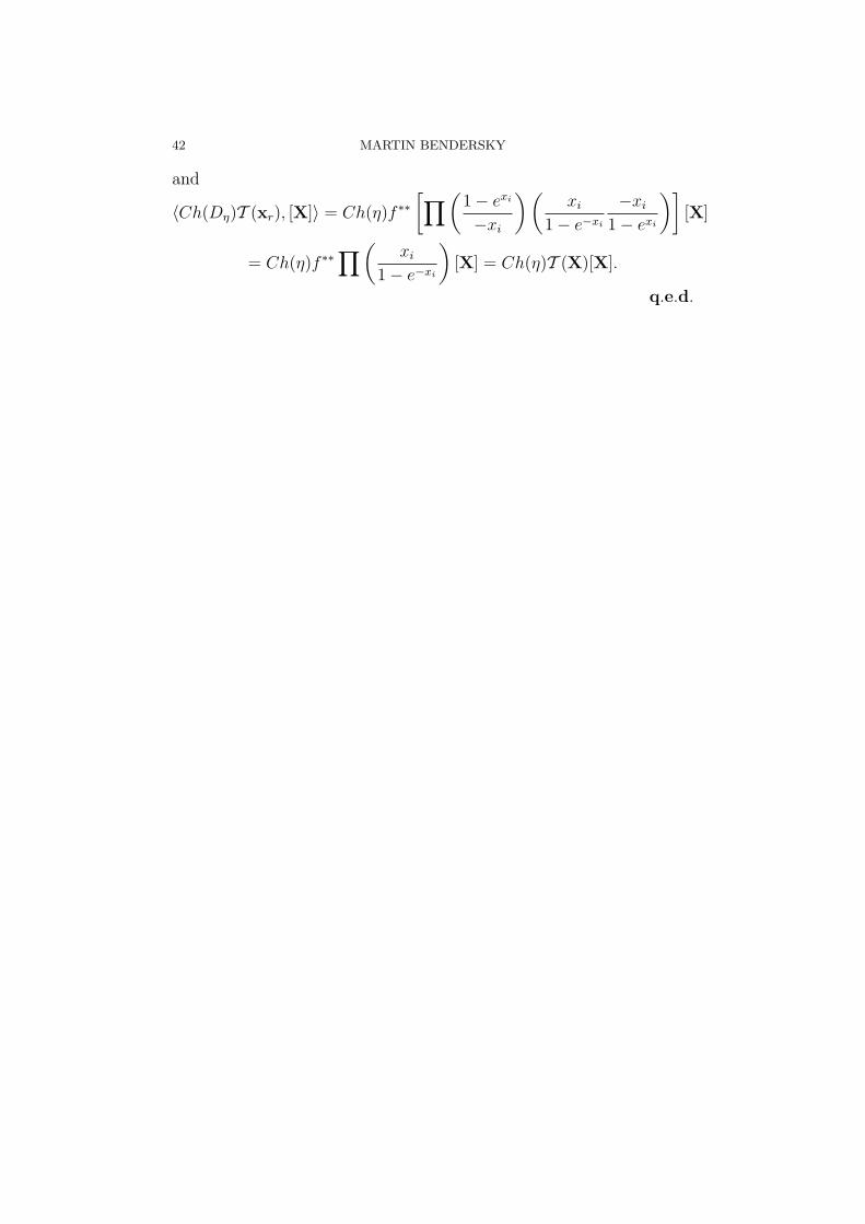
42 MARTIN BENDERSKY

and

〈Ch(Dη)T (xr), [X]〉 = Ch(η)f ∗∗[∏ (

1− exi

−xi

)(xi

1− e−xi

−xi

1− exi

)][X]

= Ch(η)f ∗∗∏ (

xi

1− e−xi

)[X] = Ch(η)T (X)[X].

q.e.d.


References

[A] Atiyah, K-theory[H] Husemoller, Fibre bundles[ABS] Atiyah, Bott, Shapiro, Clifford Modules, Topology 3 (supplement 1) (1964)[BH] A. Borel, F. Hirzebruch Characteristic classes and homogeneous spaces:

I,II,III, Am. J. Math, 80: 458-538 (1958), 81:315-382 (1959), and 82: 491-504(1960).

[MS] Milnor, Stasheff Lectures on Characteristic Classes[P] Palais, Seminar on the Atiyah Singer Index Theorem Princeton University

Press, 57[ST] Singer and Thorpe, Lecture Notes on Elementary Topology and Geometry[S] S. Sternberg, Lectures on Differential Geometry

E-mail address: [email protected]

Hunter College and Graduate Center, CUNY, New York, NY 10021

applications of elliptic operators and the atiyah singer index

Documents