applications of game theory and microeconomics in
TRANSCRIPT

Applications of Game Theory and
Microeconomics in Cognitive Radio and
Femtocell Networks
by
Mohsen Nadertehrani
A thesis
presented to the University of Waterloo
in fulfillment of the
thesis requirement for the degree of
Doctor of Philosophy
in
Electrical and Computer Engineering
Waterloo, Ontario, Canada, 2013
©Mohsen Nadertehrani 2013

ii
AUTHOR'S DECLARATION
I hereby declare that I am the sole author of this thesis. This is a true copy of the thesis,
including any required final revisions, as accepted by my examiners.
I understand that my thesis may be made electronically available to the public.

iii
Abstract
Cognitive radio networks have recently been proposed as a promising approach to
overcome the serious problem of spectrum scarcity. Other emerging concept for innovative
spectrum utilization is femtocells. Femtocells are low-power and short-range wireless access
points installed by the end-user in residential or enterprise environments. A common feature
of cognitive radio and femtocells is their two-tier nature involving primary and secondary
users (PUs, SUs). While this new paradigm enables innovative alternatives to conventional
spectrum management and utilization, it also brings its own technical challenges.
A main challenge in cognitive radio is the design of efficient resource (spectrum) trading
methods. Game and microeconomics theories provide tools for studying the strategic
interactions through rationality and economic benefits between PUs and SUs for effective
resource allocation. In this thesis, we investigate some efficient game theoretic and
microeconomic approaches to address spectrum trading in cognitive networks. We propose
two auction frameworks for shared and exclusive use models. In the first auction mechanism,
we consider the shared used model in cognitive radio networks and design a spectrum trading
method to maximize the total satisfaction of the SUs and revenue of the Wireless Service
Provider (WSP). In the second auction mechanism, we investigate spectrum trading via
auction approach for exclusive usage spectrum access model in cognitive radio networks. We
consider a realistic valuation function and propose an efficient concurrent Vickrey-Clarke-
Grove (VCG) mechanism for non-identical channel allocation among r -minded bidders in
two different cases.
The realization of cognitive radio networks in practice requires the development of
effective spectrum sensing methods. A fundamental question is how much time to allocate
for sensing purposes. In the literature on cognitive radio, it is commonly assumed that fixed

iv
time durations are assigned for spectrum sensing and data transmission. It is however
possible to improve the network performance by finding the best tradeoff between sensing
time and throughput. In this thesis, we derive an expression for the total average throughput
of the SUs over time-varying fading channels. Then we maximize the total average
throughput in terms of sensing time and the number of SUs assigned to cooperatively sense
each channel. For practical implementation, we propose a dynamical programming algorithm
for joint optimization of sensing time and the number of cooperating SUs for sensing
purpose. Simulation results demonstrate that significant improvement in the throughput of
SUs is achieved in the case of joint optimization.
In the last part of the thesis, we further address the challenge of pricing in oligopoly
market for open access femtocell networks. We propose dynamic pricing schemes based on
microeconomic and game theoretic approaches such as market equilibrium, Bertrand game,
multiple-leader-multiple-follower Stackelberg game. Based on our approaches, the per unit
price of spectrum can be determined dynamically and mobile service providers can gain
more revenue than fixed pricing scheme. Our proposed methods also provide residential
customers more incentives and satisfaction to participate in open access model.

v
Acknowledgements
I am thankful to Allah, the most merciful and most compassionate for blessing me with
the strength to seek knowledge and complete this work.
I would like express my deep gratitude to my supervisor, Professor Murat Uysal for
providing guidance throughout my PhD studies. He is a brilliant Professor with solid
theoretical and practical knowledge. I am grateful for his insightful suggestions, valuable
discussions and advices. Also I want to express my sincere gratitude to my co-supervisor
Professor Mohamed Ossuama Damen, without his help, this work would not be completed.
I would like to thank the members of my dissertation committee, Professors Oleg
Michailovich, Pin-Han Ho, Kate Larson, who despite their busy schedules accepted to review
my thesis and providing me with valuable suggestions. I am also thankful to Professor Robin
Kohen for attending my PhD examination as the delegate of Professor Larson.
Finally, and most importantly, I thank my parents, for their endless love and support,
without which I would not have succeeded. My special thanks and sincere appreciation are
extended to the love of my life, my wife, Zahra Ashouri, for all her love and understanding
during the course of my PhD.

vi
Table of Contents
AUTHOR'S DECLARATION ....................................................................................................... ii
Abstract .......................................................................................................................................... iii
Acknowledgements ......................................................................................................................... v
Table of Contents ........................................................................................................................... vi
List of Figures ................................................................................................................................ ix
List of Abbreviations ..................................................................................................................... xi
List of Notations .......................................................................................................................... xiii
Chapter 1 Introduction ................................................................................................................... 1
1.1 Motivation ................................................................................................................................. 1
1.2 Spectrum Access Models in Two-Tier Networks ..................................................................... 4
1.3 Microeconomics Theory and Its Applications in Two-Tier Networks ..................................... 6
1.4 Game Theory and Its Applications in Two-Tier Networks ...................................................... 9
1.5 Sensing Throughput Trade-off in Cognitive Radio Network ................................................. 10
1.6 Outlines and contributions ...................................................................................................... 12
Chapter 2 Spectrum Trading for Risky Environments in IEEE 802.22 Cognitive Networks .... 17
2.1 Introduction ............................................................................................................................. 17
2.2 System Model ......................................................................................................................... 17
2.3 Proposed Auction Mechanism ................................................................................................ 19
2.4 Sensing-Revenue Trade-off .................................................................................................... 22
2.5 Numerical Results ................................................................................................................... 24
Chapter 3 Sensing-Throughput Tradeoff in Cognitive Radio Networks with Cooperative
Spectrum Sensing over Time-Varying Fading Channels .............................................................. 29
3.1 Introduction ............................................................................................................................. 29
3.2 System Model ......................................................................................................................... 30

vii
3.3 Sensing Statistics .................................................................................................................... 31
3.4 Problem Formulation for Sensing-Throughput Tradeoff ........................................................ 34
3.5 Proposed Solution ................................................................................................................... 36
3.6 Numerical Results ................................................................................................................... 40
Chapter 4 Spectrum Trading for Concurrent Non-Identical Channel Allocation in Cognitive
Radio Networks ............................................................................................................................ 48
4.1 Introduction ............................................................................................................................ 48
4.2 System Model and Problem Formulation ............................................................................... 50
4.2.1 Case 2: r -minded bidders with bundle channel auction ........................................... 54
4.3 Sub-Optimal Solutions for Case 2 .......................................................................................... 57
4.3.1 Greedy Algorithm ...................................................................................................... 57
4.3.2 Randomized Rounding Relaxed LP (RRRLP) Algorithm ........................................ 58
4.4 Truthful Iterated Greedy Algorithm for Case 2 ...................................................................... 60
4.5 Simulation Results .................................................................................................................. 63
Chapter 5 Pricing for Open Access Oligopoly-Market Femtocell Networks ............................... 70
5.1 Introduction ............................................................................................................................ 70
5.2 System Model and Problem Formulation ............................................................................... 71
5.3 Pricing Schemes ...................................................................................................................... 74
5.3.1 Market Equilibrium ................................................................................................... 74
5.3.2 Bertrand Game .......................................................................................................... 78
5.3.3 Multiple Leader Multiple Follower Stackelberg Game............................................. 80
5.3.4 Cooperative Game ..................................................................................................... 83
5.4 Information Exchange Protocol and Price Determination ...................................................... 84
5.5 Simulation and Numerical Results.......................................................................................... 87
Chapter 6 Conclusions and Future Work ...................................................................................... 93

viii
6.1 Conclusions ............................................................................................................................. 93
6.2 Future Works .......................................................................................................................... 95
Appendix A Proof of Theorem 3.1 .............................................................................................. 97
Appendix B Proof of Theorem 3.2 .............................................................................................. 99
Appendix C Proof of Theorem 4.1 ............................................................................................. 101
Appendix D Proof of Theorem 4.2 ............................................................................................. 102
Appendix E Solving Linear Equations in (5.9) ........................................................................... 104
Bibliography ............................................................................................................................... 106

ix
List of Figures
Figure 2.1 Markov chain model .............................................................................................. 18
Figure 2.2 Average payoff for the SUs ................................................................................... 25
Figure 2.3 Revenue of the auctioneer in terms of sensing time for the proposed auction
model....................................................................................................................................... 26
Figure 2.4 Throughput of SUs in terms of sensing time for the proposed auction model. ..... 27
Figure 2.5 Total revenue of auctioneer in terms of the number of SUs for different sensing
times. ....................................................................................................................................... 28
Figure 3.1 Throughput of SUs in terms of sensing time ......................................................... 41
Figure 3.2 Throughput of SUs in terms of the number of SUs ............................................... 42
Figure 3.3 Optimum sensing time of SUs over single channel in terms of SNR ................... 43
Figure 3.4 Optimum Throughput for SUs over single channel in terms of SNR ................... 44
Figure 3.5 Throughput of SUs over time varying channels with different Doppler values. ... 46
Figure 3.6 Throughput of SUs for the proposed method ........................................................ 47
Figure 4.1 Average revenue of the auctioneer in case 1, i.e., the SUs are r -minded but they
can submit bid only for single channels. ................................................................................. 65
Figure 4.2 Average revenue of auctioneer in case 2, i.e., the SUs are r -minded and they can
submit bid for bundles of channels. ........................................................................................ 66
Figure 4.3 Average total social welfare in case 2. .................................................................. 67
Figure 4.4 Average revenue of bidders in case 1. ................................................................... 68
Figure 4.5 Average revenue of bidders in case 2. ................................................................... 69
Figure 5.1 Geographical distribution of FAPs under HSPP and CSPP assumptions. ............ 72
Figure 5.2 Cellular Network underlaid with femtocell network ............................................. 73
Figure 5.3 Supply and Demand function in terms of price for service provider 1. ................ 88
Figure 5.4 Bertrand Game and Multiple-leader-multiple-follower Stackelberg game .......... 89

x
Figure 5.5 Nash Equilibrium for Cooperative game .............................................................. 90
Figure 5. 6 Total profit of service providers from different methods ..................................... 91
Figure 5.7 Spectrum price in terms of spectrum substitutability (v) ..................................... 92
Figure C.1 Modeling r-minded bidders in case 2………………………...………..……… 101

xi
List of Abbreviations
WRAN Wireless regional area network
SU Secondary user
PU Primary user
MBS Macrocell base station
FAP Femtocell access point
MUE Macrocell user equipment
WSP Wireless service provider
DFC Data fusion center
FUE Femto user equipment
CA Close access
OA Open access
HA Hybrid access
QoS Quality of service
VCG Vickrey-Clark-Grove
OFDMA Orthogonal frequency division multiple access
CLT Central limit theorem
FCC Federal communication commissions
LP Linear programming
BS Base station
CDF Cumulative distribution function
PDF Probability density function
CU Currency Unit
iid Independent identical distribution
CSCG Circularly symmetric complex Gaussian

xii
PSD Power spectral density
GPS Global positioning system
MCKP Multiple choice knapsack problem
RRRLP Randomized rounding relax linear program
RR Randomized rounding
RLP Relax linear programming
HSPP Homogenous spatial Poisson process
CSSP Clustered spatial Poisson process
LTE Long term evoultion
SNR Signal to noise ratio
MLMF Multiple leader multiple follower
NE Nash equilibrium
QAM Quadrature amplitude modulation

xiii
List of Notations
N Number of SUs
fP Probability of false alarm
mP Probability of miss
uP Probability of correct detection when PU does not exist
dP Probability of detection
g Transition probability from idle to idle state in Markov model
a Transition probability from idle to busy state in Markov
model
( )idleP j Probability of the channel being in the idle state at the
beginning of the thj time interval
( )sidleP j Probability of the channel being in the idle state at the during
of the thj time interval
ix Valuation of the thi bidder
ib Bid of the thi bidder
( )ih x Valuation of the thi bidder in the presence of interference
C Channel Capacity
iD Data traffic of the thi bidder
1Y Highest order statistic
. Stands for the derivative operation
( )R xb Optimal bidding function
( )xm Revenue of service provider
Threshold for the detector
.Q Gaussian Q function
L Number of SUs
K Number of channels
xiv
0H Absence of PUs
1H Presence of PUs
( )s n Rectangular M-QAM modulated signal
( )iu n Noise samples
( )ih n Fading coefficients
R ( )ih n Real part of fading coeficinets
I ( )ih n Imaginary part of fading coefficients
T Length of frame
Sensing time
( )iy Sensing statistic d
Convergence in distribution
.iR Average throughput
df Doppler frequnecy
*i Optimum sensing time
M Number of non-identical channels
Set of all possible ways in which M non-identical channels
can be allocated to N SUs.
j Particular channel allocation
K i Set of channels in the bundle allocated to the thi bidder
m Number of channels in a bundle
K( )i iV Valuation function of the thi bidder
ip Payment of the thi bidder
(K )iiB Bid of the thi bidder for the channel allocation K i
(.)SW Social welfare function
diD Delay sensitive data traffic
d Mean of Poisson distribution of delay sensitive data

xv
oiD Delay insensitive data traffic
o Mean of Poisson distribution of delay sensitive data
1iB Bid vector of the thi bidder in case 1
1B N M Bid matrix in case 1
1,i jb Bid of the thi bidder for the thj channel in case 1
2iB r -tuple vector of bidding of the thi bidder in case 2
2,i jb Bid of thi bidder for thj channel in case 2
A N M matrix of assignments
,i jS r M matrix of the bids of the thi bidder
| K |i Cardinality of set K i
ie Hyper-edge in a hyper-graph
in Norm of a hyper-edge
grSWF Social Welfare Function of greedy algorithm
optSWF Social Welfare Function of optimum algorithm
r Number of submitted bids
H Interior of a reference hexagonal macrocell
Cl Mean of MUE distribution
fl Mean of FUE distribution
( )S p Supply function
( )D p Demand function
b Vector of shared spectrum from all MBSs
iC Fraction of spectrum that is used for FUEs
ip Unit price for spectrum from thi MBS
iA Spectral efficiency for FUEs served by FAPs
id Fixed coefficient
v Substitutability coefficient
xvi
iw Total spectrum available for the thi MBS
iM Spectral efficiencies of MUEs served by the thi MBS
ik Spectral efficiency for MUEs served by the thi FAPs
*ip Optimum price
( )i iB -p Best response function of the thi MBS
I Number of leaders

1
Chapter 1
Introduction
1.1 Motivation
The increasing usage of bandwidth-hungry wireless applications and services has fueled
demands for radio spectrum. These resources are however fundamentally limited: First, the
physical propagation mechanisms of radio waves restrict the range of usable frequencies.
Second and perhaps more important reason is that virtually all usable radio frequencies have
already been allocated to existing applications and services, leaving little spectrum for
emerging and future wireless systems. This necessities innovative approaches for spectrum
management and utilization.
Some studies in early 2000’s [1] have pointed out underutilization for many parts of the
licensed bands. In light of the imbalance between the spectrum scarcity and spectrum
underutilization, the paradigm-shifting concept of “cognitive radio” was introduced by
Mitola [2] as a promising solution for efficient spectrum utilization. By sensing and adapting
to the wireless environment, a cognitive radio network is able to fill in the available spectrum
holes of primary (licensed) users and serve its users without causing harmful interference to
the licensed ones. An example for a cognitive network is IEEE 802.22 wireless regional area
network (WRAN) standard published in July 2011 [3]. This standard aims to utilize the TV
bands that remain largely unoccupied in many geographical areas.
Another emerging concept for innovative spectrum utilization is femtocells. Femtocells
[4] are low-power and short-range wireless access points installed by the end-user in
residential or enterprise environments. They operate in licensed spectrum to connect legacy
wireless devices to the cellular operator’s network through the end-user's broadband

2
connection. Due to the proximity between transmitter and receiver, femtocells can
significantly lower the required transmit power enabling power savings and prolonging
handset battery life. On the other hand, operators benefit from the femtocells as a method of
offloading traffic from the macrocell base station. This will result in significant reductions in
infrastructure and operational expenses. If indoor wireless usage can be absorbed into the IP
backbone through femtocell deployment, the macrocell base station can further allocate its
resources mainly to outdoor users resulting in a better overall user experience. Based on a
report published in February 2013 by Small Cell Forum [5], [6], femtocell market as a win-
win solution for both end-users and operators will experience a significant growth over the
next few years
A common feature of cognitive radio and femtocells is their two-tier nature involving
primary and secondary users (PUs, SUs). While this enables innovative alternatives to
conventional spectrum management and utilization, it also brings its own technical
challenges. A main challenge in cognitive radio is the design of efficient resource trading
methods [7]. Based on the underlying technologies, resource can refer to frequency band,
channel access time, transmission power etc. In this context, trading refers the process of
selling and buying available resources in an incentive driven framework. In spectrum
(resource) trading, the objective of PUs is to maximize their revenue by selling the available
spectrum to SUs. On the other hand, the objective of SUs is to have access to the spectrum at
a reasonable price while maximizing their satisfaction (i.e., maximizing the associated utility
function). However, these objectives generally conflict with each other. Therefore, an
optimal and stable solution in terms of price and allocated resources is required so that the
revenue and utility are maximized, satisfying both the seller and the buyer [8].
Femtocell network comprises of operator-installed Macrocell Base Stations (MBS)
underlaid with short-range consumer-installed Femtocell Access Points (FAPs). This two-tier

3
network structure with cross-tier (between femtocell tier and macrocell tier) and co-tier
(among femtocell tiers) interference differ significantly from the conventional cellular
architecture that relies on the careful network planning. Operating in the same licensed band,
femtocell tier will inevitably impact macrocell tier. Resource allocation in such an
interference-limited environment poses itself as a major technical challenge for the femtocell
network design. In femtocell networks, macrocell user equipments (MUEs) can improve
indoor reception with better voice service coverage and higher data throughput with
connection to the FAPs and use their resources. Therefore innovative pricing models should
be designed to tempt users to participate in these types of communication.
The problems of spectrum trading in cognitive networks and pricing in femtocells have
attracted a growing attention in recent years. While some initial works rely on classical
optimization [8], game theory and microeconomics theory provide some alternative
mathematical tools for spectrum trading [8-9]. Game theory is a mathematical framework for
the analysis of “conflict and cooperation between intelligent rational decision makers” [11].
It was originally introduced by Cournot in 1838 [12] and, since then, has been applied to
various problems in a wide range of disciplines including economics, political science,
philosophy, computer science, engineering, etc [11]. It therefore emerges as a natural design
methodology for resource allocation in wireless networks where there are different rational
entities with different types of demands and has been used in the past for various problems in
wireless system and network design, see e.g., [12–15]. Microeconomics theory is a branch
of economics that studies the behavior of how the agents in a market1 make decisions to
allocate limited resources2 [16-17]. Its origins go back to Bernoulli’s work in 1965 [19] and
1 A market consists of sellers and buyers of commodities or services with an efficient pricing scheme to maintain the stability of market [7]. 2 A resource is any physical or virtual entity of limited availability that needs to be consumed to obtain a benefit from it.

4
has also been applied to some engineering problems such as in risk-return evaluation,
conflicting interests, etc. [20].
In this thesis, we will investigate the strategic interactions between PUs and SUs through
game theoretic and microeconomic approaches and propose solutions for spectrum trading,
and pricing in two-tier networks such as IEEE 802.22 and femtocell networks with different
access models.
1.2 Spectrum Access Models in Two-Tier Networks
In cognitive radio networks, spectrum management allows wireless systems to
dynamically access/share the radio spectrum on a negotiated or an opportunistic basis. In
exclusive-usage model, spectrum privileges are sold to commercial entities who have the
right for exclusive usage under certain rules. Spectrum owner provides service to the PUs
and sells the unused extra spectrum to the other wireless service providers (WSPs) for a
specific period of time. If, within the leasing duration, the spectrum owner needs spectrum, it
must wait until the end of lease period. Therefore in this model, cognitive systems do not
need to sense or dynamically change the spectrum.
In shared used model, on the other hand, the spectrum owned by a licensee is
simultaneously shared by a non-license holder. Such sharing takes place without the PUs
being aware of SUs. Therefore, the transmissions of SUs are expected to have minimal
impact on PUs devices. In practice, this requires that SUs should continuously sense the
spectrum, find opportunities for transmission, and vacant the spectrum if any PU wants to
enter the spectrum. Therefore, the practical implementation of cognitive radio networks
requires the development of effective spectrum sensing methods [21]. Spectrum sensing can
be either performed by a single SU or a number of cooperating SUs. In the latter one which is
named as “cooperative sensing”, SUs cooperatively perform spectrum sensing [2] and send

5
the sensing results to a data fusion center (DFC). The DFC combines the results and makes a
decision. In the literature on cognitive radio, it is commonly assumed [7-12] that fixed time
durations are assigned for spectrum sensing and data transmission. If SUs spend more time
on spectrum sensing, the probability of missing PUs will be decreased, but that also reduces
the time for data transmission. On the other hand, if they spend more time on data
transmission and less time on spectrum sensing, the probability of missing PUs and
interfering with them will increase and therefore the data throughput will decrease.
Therefore, there is a fundamental tradeoff between sensing time and throughput of cognitive
radio networks which will be further discussed within this thesis.
In femtocell networks, both of the aforementioned models can be used. In exclusive
usage model, MBS divides spectrums in two parts and allocates one part to the MUEs and
the other to Femtocell User Equipments (FUEs). In this model, there is no interference
between MUEs and FUEs. But inefficiency of spectrum utilization brings the fact that shared
use model is more desirable in femtocell networks. In a femtocell network based on the
shared use model, the spectrum is shared between the FUEs and MUEs. In this model, the
FUEs can utilize spectrum with lower priority than MUEs. Therefore interference
management becomes a critical design factor in the practice.
Another type of access in femtocell networks can be defined based on closeness or
openness of FAPs. In close access (CA), limited number of users such as family members or
friends can connect to the FAP. On the other hand, it is possible to have open access (OA)
where all customers of the operator have the right to make use of any FAP. The use of OA in
fact reduces the interference problems encountered in the case of CA. Indeed, all nearby
MUEs would be authorized to connect to any FAP, reducing thus the negative impact of the
femtocell tiers on the macrocell network. In this case, the MUEs are always connected to the
strongest server (either macro or femto), avoiding cross-tier interference. As a result, the

6
overall throughput of the network increases. OA is therefore advantageous from the operator
point of view.
From the user point of view, CA is obviously preferred who will have full control over
the list of authorized users. However, some surveys indicate that OA might be an attractive
business model for home market conditioned that competitive pricing is offered [4]. Hybrid
access (HA) methods are also discussed to reach a compromise between the impact on the
performance of subscribers and the level of access that is granted to non-subscribers.
Therefore, the sharing of FAPs resources between subscribers and non-subscribers needs to
be finely tuned. Otherwise, subscribers might feel that they are paying for a service that is to
be exploited by others. The impact to subscribers must thus be minimized in terms of
performance or via economic incentives. With a proper pricing model, deploying OA or HA
model is more beneficial for network operators than CA.
1.3 Microeconomics Theory and Its Applications in Two-Tier Networks
Microeconomics theory provides some effective pricing schemes to maintain the
stability of the market. There are two types of markets in terms of the number of sellers.
Monopoly market is the simplest market structure when there is only one seller. Oligopoly
market is the case when there are multiple sellers and multiple buyers in the market. The
sellers compete with each other independently to achieve the highest revenue by controlling
the quantity or the price of the supplied commodity. Spectrum trading in two-tier network
can be modeled as a monopoly or oligopoly market based on the number of PUs. When there
is a single PU as a seller and several SUs as buyers, monopoly market is used. Oligopoly
market is used when there exist several PUs and several SUs.
An efficient pricing scheme derived from microeconomics theory should satisfy both
buyers and sellers side. Market equilibrium and auction theory are the two popular pricing

7
schemes used for resource trading [9]. In recent studies [22]–[27], they have been applied to
spectrum trading problem in cognitive radio networks and femtocells. The market
equilibrium gives the spectrum price and allocated spectrum size for which spectrum demand
equals to spectrum supply. At the market equilibrium, the profit of the seller and the
satisfaction of the buyer(s) are maximized [22], [23]. An example of this approach for
spectrum trading is presented in [28], where hierarchical bandwidth sharing in a cognitive
radio network is considered. In [23], Dusit et.al proposed market equilibrium as a pricing
scheme for spectrum sharing in cognitive radio network and compared this method with
competitive and cooperative pricing in terms of revenue for service provider and satisfaction
of buyers.
Auction theory provides another framework for resource trading problems. An auction is
a process used to obtain the price of a commodity with an undetermined value [19]. Sellers
use auctions to improve revenue by dynamic pricing based on buyer demands. Buyers benefit
since auctions assign resources to buyers who value them the most. There are different kinds
of auctions such as English auction, sealed bid first price auction, sealed bid second price
auction (Vickery auction), double auction [29]. In the English auction, the minimum price is
set by the auctioneer. Then, a bidder submits a bid higher than the minimum price to the
auctioneer. Each bidder may observe the bids from other bidders and competes by increasing
its bidding price. Thereafter, the bidding price is continuously increased until the bidder with
the highest bidding price wins the auction. In a sealed-bid auction, all bidders submit sealed
bids independently. The auctioneer opens the bids and determines the winning bidder whose
bidding price is the highest. For the winning bidder, the price to pay the auctioneer becomes
its bidding price (i.e., first-price auction) or the second highest bidding price (i.e., second-
price auction or Vickrey auction). In a double auction, multiple buyers bid to buy
commodities from multiple sellers.

8
In [24], Vickrey auction and English auction are used for allocating unused spectrum
bands to SUs based on a guaranteed quality-of-service (QoS) assuming time-variant number
of SUs and PUs. In [7], a hierarchical spectrum trading model is presented to analyze the
interaction among the secondary service providers, TV broadcasters, and SUs. Furthermore,
a double auction with a joint spectrum bidding and service pricing model is proposed among
multiple TV broadcasters and secondary service providers who sell and buy the radio
spectrum. In [25], spectrum auction mechanisms are investigated when multiple units of
spectrum are available and the demand from SUs exceeds the available spectrum. Sequential
and concurrent auctions are further studied. In the sequential auction, all the bidders submit
their bids for all the channels simultaneously while in the concurrent auction the channels are
auctioned one after another. In [26], the spectrum allocation is modeled as a sequential
dynamic game and a pricing-based distributive collusion-resistant spectrum allocation is
proposed.
In [30], user incentives for the adoption of femtocells and their resulting impact on
network operator revenues are studied. The work in [29] models a monopolist network
operator who offers two models of access (shared use and exclusive usage) to a population of
users with linear valuations for the data throughput. It further compares the revenue from
these two models and demonstrates that shared use yields revenue comparable or higher than
that in exclusive usage. In another work on femtocells [31], the Dutch auction is used for the
design of sub-channel and power allocation scheme when femtocell users co-exist with
OFDMA macrocell users. In [32], Vickrey-Clark-Grove (VCG) auction is proposed as the
pricing scheme for OA femtocells. In [33], a reverse auction (one-buyer-multiple-sellers)
framework is proposed based on VCG mechanism for access permission trading between
wireless service provider and private femtocell owners.

9
1.4 Game Theory and Its Applications in Two-Tier Networks
A classical optimization problem consists of a single objective under a set of constraints.
while in a game model, several entities are involved with different interests [8]. The solutions
of the game should satisfy all of the entities. A game has three fundamental components: A
set of players, a set of strategies, and a set of payoffs for a given set of actions [17]. Players
are the entities who make the decisions. Strategies are a set of rules to make a decision that
defines an action for a player. Payoff (or revenue) of a player shows the satisfaction level of a
player for a given strategy. The satisfaction of the players is usually shown by a utility
function. In game theory, steady-state conditions are known as Nash equilibrium. Nash
equilibrium is a set of strategies, one for each player, such that no player has incentive to
unilaterally change his/her action.
Based on the cooperation between players, a game can be categorized in two groups as
non-cooperative and cooperative games [9]. In a non-cooperative game, each player acts as
an individual rational entity to maximize its payoff and make decisions independently. But in
cooperative games, all players in a group act as a single entity. They do not have any
competition between each other and do aim to maximize the total revenue of group. There
are also other types of game that have been extensively used for resource allocation in
cognitive radio networks such as Cournot game [34], Bertrand game [35], Stackelberge
game, dynamic/repeated game [36], stochastic game [37], bargaining game [15], coalition
game [38], game with learning [39].
In [30], the evolution and the dynamic behavior of SUs are modeled using the theory of
dynamic game. Deterministic and stochastic models are used as dynamic evolutionary
games. It is assumed in [29] that a SU does not have any intention to influence the decision
of other SUs in the future and PU uses an iterative algorithm for strategy adaptation using the
10
local information of that PU and information available to that PU from the SUs. In [40], a
solution for joint sub-channel assignment, adaptive modulation, and power control for a
multi-cell multi-user OFDMA cognitive radio network is proposed using a distributed non-
cooperative game. A virtual referee is introduced to improve the performance of the Nash
equilibrium points. This referee can modify the rule of the resource competition game for
efficient resource sharing. In [41], an optimum channel and power allocation scheme is
proposed based on the Nash bargaining solution for an OFDMA cognitive radio network.
This paper takes into account limits on the total interference for each PU as well as the
minimum SNR requirement for SUs. In [23], three different pricing models (namely, market-
equilibrium, competitive, and cooperative pricing models) are investigated for spectrum
allocation in cognitive radio networks.
Game theory has been also applied to some femtocell design problems. In [36], a utility-
based non-cooperative game is proposed for femtocell signal-to-interference-noise-ratio
(SINR) adaptation. The adaptation forces stronger femtocell interferers to obtain their SINR
equilibriums closer to their minimum SINR targets, while femtocells causing smaller cross-
tier interference obtain higher SINR margins. In [42], a game theoretic approach is used to
design decentralized resource allocation mechanisms for FAPs. In [43], a unique and fair
Pareto1 optimal operation is proposed for femtocell networks under certain minimum QoS
requirements using Nash bargaining solution.
1.5 Sensing Throughput Trade-off in Cognitive Radio Network
As earlier noted in Section 1.2, the realization of cognitive radio networks in practice
requires the development of effective spectrum sensing methods. A fundamental question is
1 An outcome of a game is Pareto optimal if there is no other outcome that makes every player at least as well off and at least one player strictly better off. That is, a Pareto Optimal outcome cannot be improved upon without hurting at least one player.

11
how much time to allocate for sensing purposes. In fact, there exists a basic tradeoff between
sensing time and throughput of cognitive radio networks which will be further discussed
within this thesis. This tradeoff problem has been first investigated for non-cooperative
spectrum sensing in [44] to find the optimal sensing time so as to maximize the total average
throughput of a cognitive radio network over Rayleigh fading channels. In [45], [46], the
optimization of the sensing time is pursued to maximize the total outage probability for the
SUs, respectively, over Rayleigh and Nakagami fading channel. In [47], the optimum sensing
time is derived to maximize the SUs throughput under the Markovian traffic assumption for
SUs and limited interference for PUs.
This tradeoff problem is revisited in [44], [48]–[50] in the context of cooperative
spectrum sensing. For sensing purposes, the spectrum can be divided into several channels
and sensing can be performed separately for each channel. Particularly, in [44], Liang and
Zheng assume a fixed number of SUs which sense each channel and send the results to the
DFC for the final decision. Under this assumption, they derive the optimum sensing time. In
[48], Peh et al. assume k-out-of-M rule with a fixed M (i.e., the number of SUs) and
optimally calculate k (i.e., the minimum number of SUs required to decide about channel
occupancy) and sensing time to maximize the throughput of SUs. In [50], Zhang et al.
calculate the minimum required number of SUs in cooperative spectrum sensing to achieve a
target error bound. In [49], Peh et al. propose a method to jointly optimize sensing time and
power allocation to maximize the throughput of SUs. In [51], Zaheer et al. formulate the
sensing throughput trade-off for distributed cognitive radio as a coalition formation game
under probability of detection constraint. In [52], Wang et al. propose an evolutionary game
to calculate the optimal time for decentralize spectrum sensing to maximize throughput of
SUs.

12
The channel models in the above works [44], [48]–[50] are either quasi-static or symbol-
by-symbol independent. Specifically, in [49], a quasi-static Rayleigh fading channel is
considered and the channel coefficients are assumed constant over all the received signal
samples. In [48], it is assumed that fading changes from one symbol to another
independently. In [44], the sensing time frame (i.e., slot) is divided into several mini-slots,
which each mini-slot consists of multiple samples and the samples are from different
symbols. The channel coefficient is assumed to be constant for each mini-slot and varies
from one mini-slot to the other one independently. In [50], the sensing channel is assumed as
time-invariant during the sensing process. These are simplifying assumptions about channel
coefficients for mathematical tractability, but not realistic for most mobile scenarios.
1.6 Outlines and contributions
The outlines and original contributions of our work in each chapter are as follows:
In Chapter 2, we address spectrum trading for cognitive radio networks with shared used
model. Majority of the literature on spectrum trading have so far assumed the exclusive-
usage model, see e.g. [7], [8], [24], [25]. Instead, we consider the shared used model in the
context of IEEE 802.22 WRAN and aim to design a spectrum trading method via auction
approach. In the shared used model, SUs perform the sensing of PU spectrum in order to
detect the vacant spectrum. Spectrum sensing is a crucial function for such opportunistic
spectrum access. Existing works on spectrum trading [8], [24], [26], [53] via auction theory
typically assume that the environment is “risk”-free1 [54], but this is highly unrealistic due to
the non-ideality of spectrum sensing. However, to the best of our knowledge, there is no
spectrum trading method specifically designed for the shared used model considering the
effects of imperfect spectrum sensing.
1 In auction theory, risk refers to the unexpected variability or volatility of returns.

13
In light of these, the first specific contribution is to design a spectrum trading method to
maximize the total satisfaction for the buyers (SUs) and revenue for the Wireless Service
Provider (WSP) taking into account sensing errors. We assume that SUs do not have GPS
and Internet to access to the online TV database for spectrum opportunities and need to
perform sensing1. In our design, we consider the risk of imperfect spectrum sensing which
causes the SUs miss the presence of licensed users and interfere with them. Taking into
account this risk, we first propose a multi-unit sequential sealed-bid first-price auction to
optimize the payoff of each SU. Then, we derive an expression for the total revenue of WSP
and maximize it by optimizing the sensing time.
In Chapter 3, we return our attention on spectrum sensing which is a crucial mechanism
for cognitive networks. Recall that Chapter 2 discusses tradeoff between sensing time and
revenue and calculates the optimum sensing time to maximize the revenue of service
provider. Chapter 3 discusses tradeoff between sensing time and throughput of SUs over
time-selective channels. For time-selective fading channels, we derive an expression for the
total average throughput of SUs each of which is equipped with energy detectors for
cooperative sensing assuming different decision rules. In this derivation, we calculate the
probability of detection and false alarm through a modified version of the central limit
theorem (CLT) for correlated variables. Based on the derived throughput expression, we
formulate an optimization problem in terms of sensing time and the number of SUs assigned
to sense each channel. In terms of sensing time, it is a non-linear programming problem
which can be solved using numerical methods. On the other hand, the problem in terms of the
number of SUs is an integer programming problem. Based on this two dimensional
1 These are defined as “sensing-only TV band devices” by the Federal Communication Commissions (FCC) [55].

14
optimization problem, we propose an algorithm to jointly optimize sensing time and the
number of cooperating SUs.
Another challenge in cognitive radio networks is the spectrum trading problem for
concurrent non-identical channel allocation which is pursued in Chapter 4. In the current
literature on spectrum auctions [7], [25], [29], [56], [57], the valuation functions used for the
bidders are somehow unrealistic. In this chapter, we propose a realistic valuation function
which each channel has different values for different bidders; this leads to non-identical
channels. In [25], [58], some methods for non-identical channel cases are investigated, but
their proposed methods are not efficient. In all of them, single-minded bidders are assumed
indicating that each bidder is willing to buy only one channel and other channels have zero
values for the bidders and the losers do not have the chance of revisiting the remainder
available channels. To address this issue, we consider r -minded bidders each of which can
bid for r>1 bundles of channels in each round of auction, but is allowed to win at most one of
these bundles. Another important issue that we want to address in this chapter is truthfulness1
or incentive compatibility of combinatorial auction mechanism when the problem of
determining auction outcomes is NP-hard.
In the light of above discussions, our main contributions in this chapter can be therefore
summarized as follows: We first propose a novel realistic valuation function for the SUs
which depends on delay-sensitive traffic (e.g., voice or video) and delay-insensitive traffic
(e.g., e-mail or file transfer) as well as the capacity of each available channel. This function is
proportional to the channel capacity and the weighted summation of data traffic types.
Instead of the commonly assumed single-minded bidders, we assume that the SUs are r -
minded bidders and design an efficient VCG-based auction mechanism. In our scheme, each
1 If an auction mechanism has the property that each user should submit their true valuation if he/she wants to maximize his/her utility function, it is called truth-telling algorithm [59].

15
bidder can bid for r bundles of channels in each round of auction, but each bidder is allowed
to win at most one of these bundles. Two cases are assumed: In case 1, the SUs are r -minded
but they can submit bid only for single channels. In case 2, the SUs are r -minded and they
can submit bid for bundles of channels. We show that the first case is solvable in polynomial
time but in the other one, the problem of determining auction outcomes is NP-hard. We
propose two sub-optimal methods for solving this problem, namely greedy algorithm and
randomized rounding linear programming (LP) relaxation. Due to the sub-optimal nature of
solutions in case 2, VCG mechanism is not truthful anymore and the SUs can lie to maximize
their utilities. To address this, we further propose an auction mechanism with limited
truthfulness property, based on an iterative greedy algorithm.
In Chapter 5, we return our attention on femtocell networks. The current market in
femtocell network is mainly geared towards CA femtocells [60]. To enable the wide
deployment of OA femtocells, innovative pricing models with incentives for residential
femtocell users are required that will be pursued in this chapter. We consider oligopoly
market and propose novel utility functions for the FAPs and MBSs which include
requirements of OA femtocell networks. We take into account discounts for the FAPs which
serve the other MUEs and dynamically set the price of spectrum different from earlier works
assuming fixed pricing. Therefore, based on our defined utility function, FAPs have more
incentives to participate in OA networks. We further propose four methods of pricing for
oligopoly market based on market equilibrium, Bertrand game, multiple-leader-multiple-
follower Stackelberg game and cooperative game. Among these four methods, we show that
the approach on market equilibrium brings more revenue than the others for the FAPs. On the
other hand, the pricing scheme with the cooperative game has the best revenue for the MBSs.
We further provide comparisons with fixed pricing schemes [61] and demonstrate the
superiority of our proposed schemes in terms of revenues.

16
In Chapter 6, we first provide the conclusion of research work done so far and then
discuss some future directions.

17
Chapter 2
Spectrum Trading for Risky Environments in IEEE 802.22
Cognitive Networks
2.1 Introduction
In this chapter, we consider the shared used model and design a spectrum trading
method to maximize the total satisfaction for the buyers (SUs) and revenue for the WSP
taking into account sensing errors in TV bands. We first propose a multi-unit sequential
sealed-bid first-price auction to optimize the payoff of each SU. Then, we derive an
expression for the total revenue of WSP and maximize it by optimizing the sensing time. Our
results demonstrate that the proposed auction-based spectrum trading method brings better
revenue than its counterparts in [25], [29].
2.2 System Model
We consider a cognitive radio network which operates in TV bands and involves the
point-to-multipoint communication between a Base Station (BS) and N SUs. Under the
assumption of the shared used model, SUs and BS are responsible for sensing and finding
opportunities in the spectrum and avoiding to make interferences with the PUs (i.e., TV
channels).
There are two hypotheses for detection; namely 0H and 1H as the absence or the
presence of the PUs, respectively. Due to the imperfect nature of spectrum sensing to identify
the spectrum opportunities, we assume that there are some risks in the presence estimation of
the PUs. Four types of probability associated with imperfect sensing can be defined:

18
1) Probability of false detection ( 1 0(H | H )fP P= ),
2) Probability of miss ( 0 1(H | H )mP P= ),
3) Probability of correct detection ( 0 0(H | H )uP P= ) when PU does not exist,
4) Probability of detection when PU exists ( 1 1(H | H )dP P= ).
We model the traffic of the SUs with a Markov process [62] as illustrated in Fig.2.1. The
channel states are represented by 0 (busy) and 1 (idle). To reflect the effect of sensing, we
consider four states, namely “idle-true”, “idle-false”, “busy-true”, and “busy-false”. For
example, the state of “idle-true” indicates that the channel is decided to be idle when it is
actually in idle state. If it is decided to idle when it is actually in busy state, this is named as
“idle-false”. State transitions are based on the transition probabilities g and a in the two
states Markov process and probabilities of detection and false alarm.
Figure 2.1 Markov chain model

19
Let ( )idleP j denote the probability of the channel being in the idle state at the beginning
of the thj time interval. Furthermore, let ( )sidleP j denote the probability of being in the idle
state during the thj time interval. The latter takes into account sensing results acquired
within the thj time interval. Based on whether the channel is sensed as idle or busy, we have
1
1
1if channel is sensed as idle
1
if channel is sensed as busy
f idle
f idle idle msidle
f idle
f idle idle d
j
P j P j PP j
P j
P P j P j P
P P
P
P
(2.1)
where
1 1 1 {1,2,...}s sidle idle idlejP j P P j j . (2.2)
If the channel is sensed as idle, the auction will be held for that channel and risk related
information ( )sidleP j is announced to the SUs for their biddings. On the other hand, if the
channel is sensed as busy, no auction will be held.
2.3 Proposed Auction Mechanism
In this section, we propose a sealed-bid first-price auction1 to optimize the payoff of
each SU. In this auction type, the highest bidder wins and pays the amount he/she bids. This
auction can be carried out either in concurrent or sequential version. Sequential version has
better revenue for the auctioneer and bidders in the auctions with non-identical items [29].
Since the non-identical channels is considered, we can assume that channel conditions (such
as noise, fading and interference) will change independently in each round of auction.
Furthermore, we assume that the traffic of SUs will change independently from one round to
1 Sealed-bid second-price auction is rarely used in practice because of the possibility of cheating by the seller [8], [29]. With the fear of cheating, a second price auction may become less profitable than a first price auction for non-cheating and fair seller.

20
another round. Therefore we assume that the SUs cannot use the history of the previous
rounds of auction for their biddings in the future round of auction.
At the beginning of each time frame, the BS determines the channels and the amount of
time that SUs should sense. After sensing period, each SU sends the sensing results to the BS
using a single bit which represents the state of each channel (0 for busy and 1 for idle). The
BS makes the final decision about the channel availability and calculates the associated risk
for each channel based on (2.1) and (2.2). At the beginning of each round of auction, the BS
announces the available channel and associated risk. SUs calculate their biddings and send
them to the BS. The BS allocates the channel to the highest bidder. Since our proposed
auction method is sequential, this process is iterated in multiple rounds. Considering the data
rates supported in IEEE802.22, it can be shown that the required time for transmission of
overhead information is negligible in comparison to the sensing time [3]. Since the bidding
strategy and winner determination of the auction can be calculated in polynomial time, the
proposed spectrum trading method has a linear computational complexity with ( )O N where
N is the number of bidders.
In our proposed method, the bidder’s payoff can be expressed as
if max & risk does not occur
0 if max
( ) if max & risk occur
i i i ji j
i i ji j
i i i ji j
x b b b
b b
h x b b b
(2.3)
where ix is the valuation of the thi bidder (i.e., the maximum amount that the thj bidder is
willing to pay for the channel), ib is the bid of the thi bidder, and ( )ih x is the valuation of the
thi bidder in the presence of interference.
We assume ( )i ix C D T where C denotes the channel capacity, iD is the data
traffic of the thi bidder, T is the length of transmission frame (i.e., the total time for sensing

21
and data transmission), and is the sensing time1. The maximum channel capacity between
SUs and BSs is denoted by maxC and the maximum data traffic of SUs is defined by maxD . In
the case of interference, the channel capacity for the SUs is smaller than channel capacity
with no interference, therefore we have ( )ih x < ix .
Fix a bidder, say the first one 1x without losing generality, and let 1Y denote the highest
order statistics, i.e. 1 2max( ,..., )NY x x , among 1N- remaining bidders 2 3, ,..., Nx x x .
Clearly, for all y , 11( ) ( )N
iG Y y F x y where G (.) and (.)F respectively denotes the
cumulative distribution function (cdf) of 1Y and ix . Based on our assumptions for the
distribution of parameters, the distribution of x is assumed2 as ( )F x . Therefore the
probability density function (pdf) of 1Y can be calculated as
1( ) ( 1) ( ) ( )
Ng x N f x F x
(2.4)
where ( )f x is the pdf of x . In our proposed method, the expected payoff for an SU is given
by
( ) ( ) 1 ( ) ( ) G( )s sR idle idlem x P j x b P j h x b x . (2.5)
The optimal bidding of bidders is a function of their valuations. Let ( )R xb denote the
optimal bidding function (strategy). It can be calculated by the maximizing ( )Rm x with
respect to b , i.e.,
1
11
1 ( ) 0g ( )
( ) ( ) G ( )( )
RR
R
s sidle idle
R
jb
P j x b P h x b bb
(2.6)
where . stands for the derivative operation. After some mathematical manipulations, (2.6)
can be rewritten as
1 In this section, we assume that sensing time is fixed. In the next section, we further discuss its optimal choice to maximize the revenue. 2 We ignore index i in the following for the sake of presentation simplicity.
22
( ) ( ) ( ) ( ) ( ) 1 ( ) ( ) ( )s sR R idle idlex g x x G x P j x P j h x g x . (2.7)
Therefore, the optimal bidding function is obtained as
0
1( ) ( ) (1 ( )) ( ) g( )
G( )
x s sidle idleR x P j y P j h y y dy
x (2.8)
2.4 Sensing-Revenue Trade-off
In the previous section, we have proposed an auction mechanism to optimize the payoff
of each SU under the assumption of a given fixed sensing time. In this section, we will first
calculate the total revenue of WSP and then maximize it by optimizing the sensing time.
Fixed time durations are typically assigned for spectrum sensing and data transmission.
This is obviously not the optimal solution. If the SUs spend more time on spectrum sensing,
the probability of missing PUs decreases, but this reduces the time for data transmission and
therefore the payment of SUs to the WSP decreases. On the other hand, if they spend more
time on data transmission and less time on spectrum sensing, the probability of missing PUs
and interfering with PUs will increase. This will decrease the bidding and payment of SUs to
the WSP. Hence, there is a trade-off between sensing time and revenue that we will discuss
in the following.
SUs are mainly interested in the channels that are underutilized, such as channels with
0.5idleP . On the other hand, the total probability of detection ( dP ) is usually more than 0.7
[44] and the total probability of false alarm ( fP ) is usually small ( 0.3 ). Under the
assumption of these typical values, it is possible to ignore (1 ( )) ( )sidleP j h y in (2.8) and
approximate it as
0( )
( )
1( ) ( )
x sidleR x
G xP j yg y dy . (2.9)
The expected revenue of the WSP from an SU can be then calculated as

23
0
( )E E ( ) ( ) E ( ) ( )x s
idleRxm G x x P j yg y dy (2.10)
where the expectation is with respect to the variable y . This yields
max max ( )
0( )E ( ) ( )(1 ( ))
C D T sidlexm P j yg y F y dy
. (2.11)
The total average revenue of auctioneer is the summation of the payments of N SUs to
the auctioneer, therefore is given by Total ( ) ( )E Ex xm N m . Here, we will maximize the
total average revenue with respect to sensing time subject to adequate protection given to the
PUs. Therefore, this problem can be formulated as
Totalmax E ( )
s.t , 0d d
m x
P P T
(2.12)
where dP is the minimum probability of detection that the BS needs to achieve to protect the
PUs in the thi channel. For a given sensing time , if we have two probability of detection
values, say dP and 1dP ( 1
d dP P ), it can be shown that 1
Total TotalE ( , ) E ( , )d dm x P m x P .
Therefore we can conclude that the optimal solution of (2.12) occurs when constraint d dP P
is at equality.
Modifying the constraint and replacing (2.4), (2.5) and (2.11) in (2.12), we can rewrite it
as
max max ( )
01
1max ( )(1 ( ))
1
s.t , 0
C D Tf idle
f idle idle m
d d
P j
P j P j P
Pyg y F y dy
P
P P T
. (2.13)
In (2.13), the probability of miss and the probability of false detection are respectively
given by [55, Eqs. (13), (14)] 1m dP P and 1( , ) ( ) 2 1f d sP Q Q P f ,
where is the threshold for the detector, is the SNR for the received signal from PU, sf
is the sampling frequency and .Q is Gaussian Q function. The above problem in (2.13) is a

24
nonlinear optimization problem and can be solved by numerical methods such as interior
points method [8].
2.5 Numerical Results
In this section, we provide Monte-Carlo simulation results to demonstrate the
effectiveness of the proposed auction model. In our simulations, we use the notation of
“currency unit (CU)” instead of any particular currency. We assume that the number of
available channels for bidding is 10 and the number of bidders is between 11 and 30. The
channels will be sensed cooperatively by SUs and BS and each channel will be sensed by one
SU. Also we assume that the sensing results are sent honestly to the BS by the SUs. PU
traffic model is modeled by a two-state Markov model with 0.8g = and 0.2a = . We
assume that bandwidth of each channel is 6 MHz. The sampling frequency is the same as
signal bandwidth. The fading channel coefficients between SUs and BS are Rayleigh
distributed and noise has normal distribution with zero mean and 1s = . The traffics of SUs
are assumed to follow a Poisson distribution with a mean of 50 Kb/s. The length of
transmission frame is 100 ms.
In Fig. 2.2, we present the performance (i.e., average payoff of bidders) for the proposed
auction mechanism assuming different values of mP . As a benchmark, we include the
performance of the conventional auction method for the sealed-bid first-price auction. In the
conventional method, the SUs select their bidding strategy without considering any
uncertainties in the valuation of channels [25]. It is observed that the proposed bidding
strategy outperforms the conventional one in a risky environment. The payoff of bidders by
our proposed method is at least two times and, in the best case, five times more than that can
be obtained from the conventional one. It is also observed that when the number of SUs

25
increases, average payoff of the SUs decreases. This decrease is due to the decreasing chance
of winning for the bidders and also increases in the amount of bids.
Figure 2.2 Average payoff for the SUs
Fig. 2.3 illustrates the revenue of the auctioneer for the proposed auction method in
terms of sensing time. We assume 15N SUs and 0.1mP = . It is observed that the revenue
of auctioneer is a convex function of the sensing time and there is an optimal (in terms of
revenue maximization) sensing duration. For the given numerical values, this is found to be
8.5 ms in our case. Fig. 2.4 illustrates the throughput of SUs in terms of sensing time. It is
observed that the throughput is maximized for 33.5 ms. This clearly shows that the optimal
10 12 14 16 18 20 22 24 26 28 30-50
0
50
100
150
200
250
300
350
400
Number of SUs
Ave
rage
Pay
-ff
for
SU
s
Pmiss=0.3, Proposed MethodPmiss=0.3, Conventional Method
Pmiss=0.1, Proposed Method
Pmiss=0.1, Conventional Method
Pmiss=0.2, Proposed MethodPmiss=0.2, Conventional Method

26
sensing time that maximize the revenue of auctioneer and throughput of SUs are different
from each other.
Figure 2.3 Revenue of the auctioneer in terms of sensing time for the proposed auction
model.
0 10 20 30 40 50 60 70 80 90 1000
1
2
3
4
5
6
7
8x 10
4
Sensing Time (msec)
Rev
enue
for
the
auc
tione
er
Revenue of the auctioneer

27
Figure 2.4 Throughput of SUs in terms of sensing time for the proposed auction model.
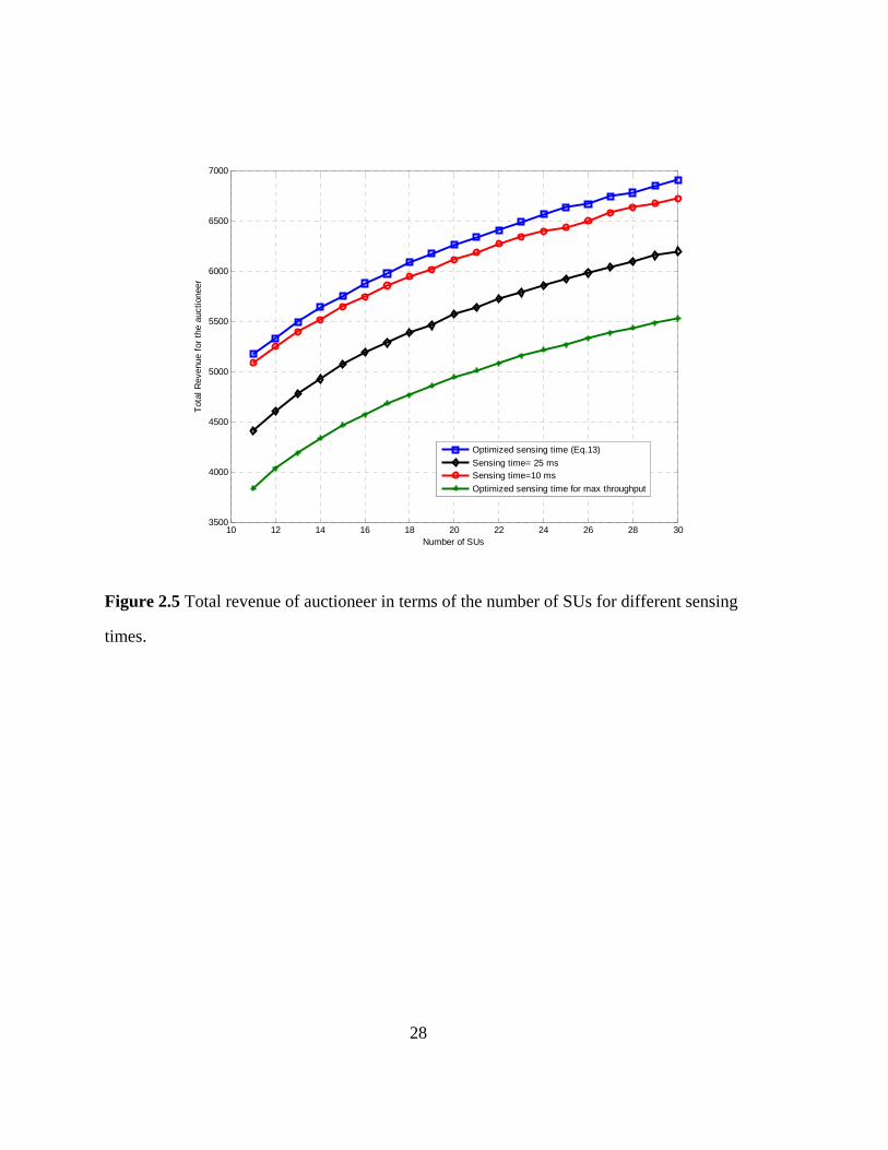
Fig. 2.5 illustrates the revenue of auctioneer in terms of the number of SUs for the
proposed auction method assuming a) different values of fixed sensing time
( 10 ms and 25 ms ), b) optimized sensing time calculated from (2.13) to maximize the
revenue, and c) optimized sensing time to maximize the throughput when the SUs are
cooperating with each other. It is observed that the total revenue of auctioneer with optimized
sensing time calculated from (2.13) outperforms the other two. The revenue of auctioneer in
this case is respectively 5% and 25% more than that can be obtained from cases (a) and (c)
while the throughput for the SUs is about 5% and 15% less. This indicates that maximizing
throughput is not necessary to get the maximum revenue.
0 10 20 30 40 50 60 70 80 90 1000
0.5
1
1.5
2
2.5
3
3.5
4
4.5x 10
4
Sensing Time (msec)
Thr
ough
put
of S
Us
Throughput of SUs
28
Figure 2.5 Total revenue of auctioneer in terms of the number of SUs for different sensing
times.
10 12 14 16 18 20 22 24 26 28 303500
4000
4500
5000
5500
6000
6500
7000
Number of SUs
Tot
al R
even
ue f
or t
he a
uctio
neer
Optimized sensing time (Eq.13)
Sensing time= 25 msSensing time=10 ms
Optimized sensing time for max throughput

29
Chapter 3
Sensing-Throughput Tradeoff in Cognitive Radio Networks with
Cooperative Spectrum Sensing over Time-Varying Fading Channels
3.1 Introduction
In Chapter 2, we have addressed spectrum trading problem for shared use spectrum
access model in IEEE 802.22. Specifically, we have considered the risk of imperfect
spectrum sensing and proposed a sequential first price auction mechanism. In our proposed
auction, the bidders calculate the optimum bidding to maximize their payoff given the risk of
imperfect sensing. We have discussed about sensing-revenue tradeoff and calculated the
optimum sensing time to maximize the revenue of auctioneer. As demonstrated, the optimal
sensing time that maximizes the revenue of auctioneer and throughput of SUs are different
from each other.
In Chapter 3, we now assume a fixed time for sensing and data transmission in shared
use spectrum access model. In this chapter, we want to address sensing-throughput tradeoff
in cognitive radio networks with cooperative spectrum sensing. The revenue of the service
provider is out of scope of this chapter and our focus is on maximizing the throughput of SUs
subject to limited interference with PUs. In this chapter, we consider a correlated fading
channel model with the well-known Jakes model for power spectral density [55]. Under this
channel model, we formulate the optimum tradeoff problem between sensing time and
throughput. We further take into account the fact that each SU cannot sense all the channels
and assume that each SU can be assigned for the sensing of a particular channel at a time and
this assignment is done on a dynamic basis. Therefore, the number of SUs assigned for
sensing of a particular channel will be determined dynamically based on the detection
performance of PUs and the channel capacity of SUs in each channel.

30
3.2 System Model
We consider a cognitive radio network with L SUs and one DFC. There are K channels
( L K ) to be sensed cooperatively by the SUs and the hard decision results will be sent to
the DFC for the final decision. As the spectrum sensing is a time consuming task, we assume
that each SU can sense only one channel during the sensing period. The assignment of SUs to
each channel is made on a dynamical basis by the DFC. During sensing time in each time
frame, the SUs are responsible to sense the assigned channels. The assigned channels to SUs
can be changed from one time frame to the other one by the DFC.
There are two hypotheses for detection; namely 0H and 1H as the absence or the
presence of the PUs, respectively. When the PU signal is present, the received sampled signal
at the thi SU can be written as
( ) ( ) ( ) ( ), 1,2,...,i i iy n h n s n u n n N (3.1)
where ( )s n is a rectangular M-QAM modulated signal and N is the number of received
signal samples. Signal samples are assumed to be independent identically distributed (i.i.d.)
random variables with zero mean and variance of 2 2E | ( ) | ss n [44]. The noise samples,
( )iu n are assumed to be circularly symmetric complex Gaussian (CSCG) i.i.d. random
variables with zero mean and variance of 2 2E | ( ) |i uu n . In (3.1), ( )ih n represents the
fading coefficient and is modeled by a complex Gaussian random variable with zero mean
and variance of 2 2E | ( ) |i hh n . Let R ( )ih n and I ( )ih n denote real and imaginary parts of
the fading coefficient. ( )ih n can be therefore written as
R I( ) Re ( ) Im ( ) ( ) ( )i i i i ih n h n j h n h n jh n . (3.2)
The autocorrelation function for the real/imaginary part of channel coefficients is defined as
def
( ) E ( ) ( ) E ( ) ( )R R I Ii i i i il h n h n l h n h n l . (3.3)

31
It should be further noted that R ( )ih n and I ( )ih n are independent of each other. The
corresponding Doppler (PSD) is obtained taking the Fourier transform of the correlation
function. For the Jakes model [55] under consideration, we have
2
1 1F ( ) = S , | |
1i i d
dd
l f f ff f f
(3.4)
where df is the Doppler frequency.
3.3 Sensing Statistics
In cognitive radio networks, the frame structure consists of two main parts. The first part
is for sensing and the second one is for data transmission. Let T denote the length of the
frame (i.e., the total time required for sensing and transmission purposes) and assume that
T is allocated for sensing. We assume that each SU employs an energy detector to
measure the received signal power during the sensing period. Let sf denote the sampling
frequency. The number of received samples is therefore given by sN f . The decision test
statistics for energy detector is expressed as
2
1
1( ) | ( ) |
N
i in
y y nN
. (3.5)
If N is large enough, the Probability Density Function (PDF) of ( )iy under hypothesis
0H can be approximated with Gaussian distribution with mean 20 u and variance
2 4 40 1 / E | ( ) |i uN u n based on the CLT [44]. Since ( )iu n is CSCG, it can be shown
that 4 4| ( ) |E 2i uu n and 2 4
0 1 / uN . The probability of false alarm is then given by
0 2( , ) Pr( ( ) | H ) 1f i s
u
P y Q f
(3.6)
where denotes the threshold of the energy detector employed at the thi SU and .Q is the
complementary distribution of the standard Gaussian [63].

32
Under hypothesis 1H , since the channel coefficients ( )ih n are correlated, ( )iy n are
correlated to each other, 1, 2,...,n N and the CLT cannot be used in a straightforward
manner. For the correlated case, we use a modified version of the CLT [64].
Theorem 3.1 (Central Limit theorem for Correlated Sequences) [64]: Let { }nx be a
stationary and mixing1 sequence of random variables satisfying a CLT condition such that
1) E ,nx n (3.7)
2) 2Var ,nx n (3.8)
3) 21
2
lim Var 2 Cov , ,n
n in
i
n x x x V n
. (3.9)
Then, a central limit theorem applies to the sample mean nx
dnx
n ZV
(3.10)
where Z is standard normal random variable and d
indicates convergence in distribution.
This theorem indicates that the CLT holds for correlated random variables but with
different variance than the independent case. In Appendix A, we prove that the received
samples ( )iy n satisfy the three conditions stated in (3.7)-(3.9) and therefore, following
(3.10), ( )iy can be approximated as a normal random variable with mean 21 u and
variance of
42 2 4 4 21
1
3 3 7 21 2 1
5 1
Nu
s h ii
M
N NM
(3.11)
1 The sequence is said to be “mixing” if the states are asymptotically independent, i.e., as the times between the measurements increase to infinity, the observed values of the measurements at those times become independent [64].

33
for large values of N. In the above, is the average received SNR at each SU and is given as
2 2 2h s u .
The probability of detection under hypothesis 1H can be now calculated as
1
2
2 2
1
( , ) Pr( ( ) | H )
13 3 7
1 2 2 15 1
d i
s
Nu
ii
P y
fQ
M
M
. (3.12)
The probability of false alarm can be written as
1 2 2
1
3 3 7( , ) ( ) 1 2 2 1
5 1
N
f d i si
MP Q Q P f
M
(3.13)
where dP denotes the target probability of detection.
In cooperative sensing, after each SU makes its individual decision denoted by iD , it
sends its result to the DFC. Here, 1iD means that there is a PU detected in the channel and
0iD means that no PU is detected. The DFC can employ OR-rule, AND-rule or majority
logic rule [21]. Let ,dP and ,fP respectively denote the probability of detection
and false alarm for each SU. The detection and false alarm probability of cooperative
spectrum sensing (i.e., , ,d k and , ,f k , respectively) for different decision rules
are calculated as
/2
1 1 ( , ) , for OR rule
( , , ) ( , ) , for AND rule
1 ( , ) ( , ) , for majority logic rule
k
d
k
d d
kk i i
d dki
P
k P
kP P
i
. (3.14)

34
/2
1 1 ( , ) , for OR rule
( , , ) ( , ) , for AND rule
1 ( , ) ( , ) , for majority logic rule
k
f
k
f f
k k i i
f fi k
P
k P
kP P
i
. (3.15)
3.4 Problem Formulation for Sensing-Throughput Tradeoff
The total average throughput is given by
1
, ,K
iT i i i
i
R R k
(3.16)
where , ,ii i iR k is the average throughput for the thi channel , 1, 2,...,i K . For the
calculation of (.)iR , we need to consider two cases based on whether DFC makes a correct
decision or not. In the first case, the DFC truly detects the absence of PUs. The second case
is that the DFC misses the presence of PUs. Let 0 , ,ii i iR k and 1 , ,i
i i iR k denote the
corresponding throughput for the ith channel. They are given by
0 0 0, , (H ) 1 1 , ,i i ii i i i f i i iR k C P T k
T
(3.17)
1 1 1, , (H ) 1 1 , ,i i ii i i i d i i iR k C P T k
T
(3.18)
where 0iC and 1
iC denote the channel capacity of the thi channel under hypothesis 0H and
1H , respectively. 0(H )iP and 1(H )iP are the probabilities of the PU being absent or present
in the thi channel, respectively. Therefore the average throughput of the SUs from the thi
channel is
0 1, , , , , ,i i ii i i i i i i i iR k R k R k . (3.19)
SUs are mainly interested in the channels that are underutilized, such as channels with
0(H ) 0.5iP . On the other hand, the probability of detection for cooperative spectrum

35
sensing ( d ) is usually more than 0.7 and 1 0.3d [44]. But the probability of false
alarm for cooperative spectrum sensing ( f ) is usually small ( 0.3 ) and therefore
1 0.7f . Thus it is possible to ignore 1 , ,ii i iR k in (3.19) and approximate (3.19) as
0, , , ,i ii i i i i iR k R k . This will yield
01
, ,K
iT i i i
i
R R k
. (3.20)
In our work, we want to maximize the average total throughput of SUs with respect to
the optimization variables, namely sensing time ( i ), the number of SUs ( ik ) and detection
threshold ( i ). Therefore we can write this optimization problem as
, ,
1
max , ,i i i
Ki
i i iki
R k
(3.21)
1
s.t. i) , ii) 0 , iii) 1 , iv) , ,K
id d i i ii i i
i
P T k K k Lk
where idP is the minimum probability of detection that the DFC needs to achieve to protect
the PUs in the thi channel. idP can take different values in each channel based on the activity,
power and sensitivity of PUs.
Lemma: Optimal solution of (3.21) occurs when the first constraint is at equality for all
decision rules.
Proof: For a given ik and i , we may choose a detection threshold 0i which satisfies
0( )i id dP . We may also choose a detection threshold 1 0
i i such that 1 0( ) ( )i id d .
Obviously from (3.13), we can conclude that 0 1i i
f f . However, we observe from
(3.17) that 0 1 0 0i i i iR R and, therefore, 1 0
i i i iR R . Hence, it proves that (.)iR will
be maximized only if ( , , ) id i i i dk P . When the first constraint in (3.21) is an equality in
all decision rules for any given pair of i , ik , we are able to determine a threshold from
(3.22) to satisfy , , id di i i
Pk which is given by

36
2 2
1 12 1
3 3 71 2 2 1
5 11 1 1i
N
ii
i ki u d
s
M
MQ P
f
. (3.22)
Using the Lemma, the problem formulation in (3.21) can be rewritten as
,
1
1
ˆmax ,
s.t. i) 0 , ii)1 , iii)
i i
Ki
i ik
i
K
i i ii
R k
T k K k L
(3.23)
where ˆ ( , )ii iR k denotes the value of , ,i
i i iR k with the threshold i chosen by (3.22).
The resulting problem is a two dimensional optimization problem whose solution will be
pursued in the following section.
3.5 Proposed Solution
In the first step, we will optimize the sensing time for a given i ik k . For each channel,
we find the optimal value of sensing time ( *i ) that maximizes the throughput of SUs in the
thi channel. The optimization problem is given as
0 0ˆmax ( ) , (H ) 1 1 ( )
s.t 0
i ii
i i i i ii i i f ik k
i
R R k C P TT
T
(3.24)
where ( )f i is the ,f i ik . We will prove that ( )iiR is a unimodal function in the
range of 0 i T for a given i ik k . If ( )iiR is a unimodal function, then ( )i
iR
monotonically increases within the range of *0 i i while it decreases within the range of
*i i T . Hence *i
iR is the only local maximum in the range of 0 i T .

37
Theorem 3.2 (Unimodal Function): If ( )iiR satisfies the following three conditions in the
range of 0 i T for a given i ik k then ( )iiR is a unimodal function.
1) (0) 0,ii i iR k k . (3.25)
2) ( ) 0,ii i iR T k k . (3.26)
3) *unique i , which *( ) 0,ii i i iR k k . (3.27)
In Appendix B, we prove that ( )iiR satisfies (3.25)-(3.27) for majority logic rule, also this
proof can be extended for OR-rule and AND-rule.
Each channel should be sensed by at least one SU, therefore there are L K
optimization problems to find *i given different values of SUs for each channel. These
optimization problems can be solved by bisection search method, or Newton’s method [65].
In total, we should solve ( )L K K optimization problem to find all *i . The second step of
our solution involves finding the optimal allocation of SUs to sense the channels with
optimum *i (that we have calculated in the previous step). Therefore the optimization
problem in the second step is given by
*
*0 0
1
1
( )max (H ) 1 1 ( ( ), )
s.t
i
Ki i i i
f i i ik
i
K
ii
kC P T k k
T
k L
. (3.28)
Let *( )i ik denote the optimum sensing time when ik SUs sense the thi channel. There
are ( 1)!/ (( 1)!( )!)L K L K cases to search and find the optimum allocation of SUs. When
L and K are small numbers, it is possible to carry out exhaustive search. But it is infeasible
for large values as the total number of cases increase exponentially. For example, for 10K
and 40L , there are more than 62 10 cases.
As an alternative to exhaustive search, we model (3.28) as a multiple choice knapsack
problem (MCKP) [66] (commonly studied in combinatorial optimization) and propose a

38
solution with low computational complexity for this step. Given a set of items each with a
weight and a value, the original knapsack problem determines the count of each item to
include in a collection so that the total weight is less than or equal to a given limit and the
total value is as large as possible [67]. The difference of MCKP from the original knapsack
problem is that in MCKP, there are multiple classes of items and exactly one item must be
taken from each class. We will use dynamic programming for the solution of (3.28). The
main idea is first to break down a complex problem into simpler sub-problems, then find
solutions for the sub-problems and finally combine these solutions to reach the overall
solution.
In our case, we want to assign SUs to the channels as to maximize the total average
throughput. In an analogy to the MCKP, K different sets represent K different channels and
the total weight of knapsack represents the total number of SUs (i.e., L ). The weight of the
thi item in the thj set is the number of SUs assigned to sense the thj channel and the value of
the item is the throughput calculated from (3.24). In the first step of our proposed solution,
we calculate the throughput for any possible allocation of SUs to each channel; therefore we
know all the weights and all the values for the set of items. In the second step, we will solve
the MCKP using dynamic programming.
Eq. (3.28) can be rewritten in the form of MCKP as
, ,1 1
,1 1
,1
,
max
i)
s.t ii) 1, 1, 2,...,
iii) 0,1 , 1,2,..., , 1, 2,...,
i
K L K
i j i jk
i j
K L K
i ji j
L K
i jj
i j
R a
ja L
a i K
a i K j L K
(3.29)

39
where ,i jR is the throughput of the SUs in the thi channel when j SUs are assigned for
sensing of the channel. ,i ja will be 1 if j SUs assigned for the sensing of the thi channel,
otherwise set to 0. The second constraint ,11
L K
i jia
means that at least one SU should be
assigned for the sensing of each channel. The first constraint ,1 1
K L K
i ji jja L
indicates
that the total number of SUs for the sensing of the channels is L .
Based on (3.29), we propose a dynamic programming algorithm for solving our MCKP.
The steps of the algorithm are provided in Table 3.1. In the first step, we initialize three
matrices, namely V (valuation), a (assignment) and Index with the size of ( )K L K´ - . In
first step, we solve the knapsack problem for 1i = (i.e., the number of sets) and different
number of SUs (i.e., the weight in knapsack problem) for 1 j L K£ £ - . In the second step,
we use ( ) ( )( ) ( )max 1,1: , : 1 :1 , 1V i j R i j V i j- + - > - to find ( , )V i j and ( , )Index i j for
each i and j . Therefore we find ( , )V K L K- (which is the optimum value of (3.29)) and
( , )Index K L K- in this step. In the third step, we use backward induction to find ( , )a i j for
each channel. Specifically, we start from ( , )Index K L K- ; if ( , ) 0Index K L K- > then
( , ( , )) 1a K index K L K- = which means that the thK channel should be sensed by a number
of SUs i.e., ( , )index K L K- . After that we use ( , ); 1;j j Index i j i i= - = - to update the
parameters i , j and find the number of sensing SUs for other channels.

40
Table 3.1 Proposed algorithm for MCKP
3.6 Numerical Results
In our simulation study, we assume a cognitive radio network with different number of
SUs and channels for sensing. The bandwidth of each channel is 6 MHz. The sampling
frequency is the same as signal bandwidth. The received SNR from PUs signals varies in
each channel and its mean takes values within the range of 25 dB and 0 dB. The inactivity
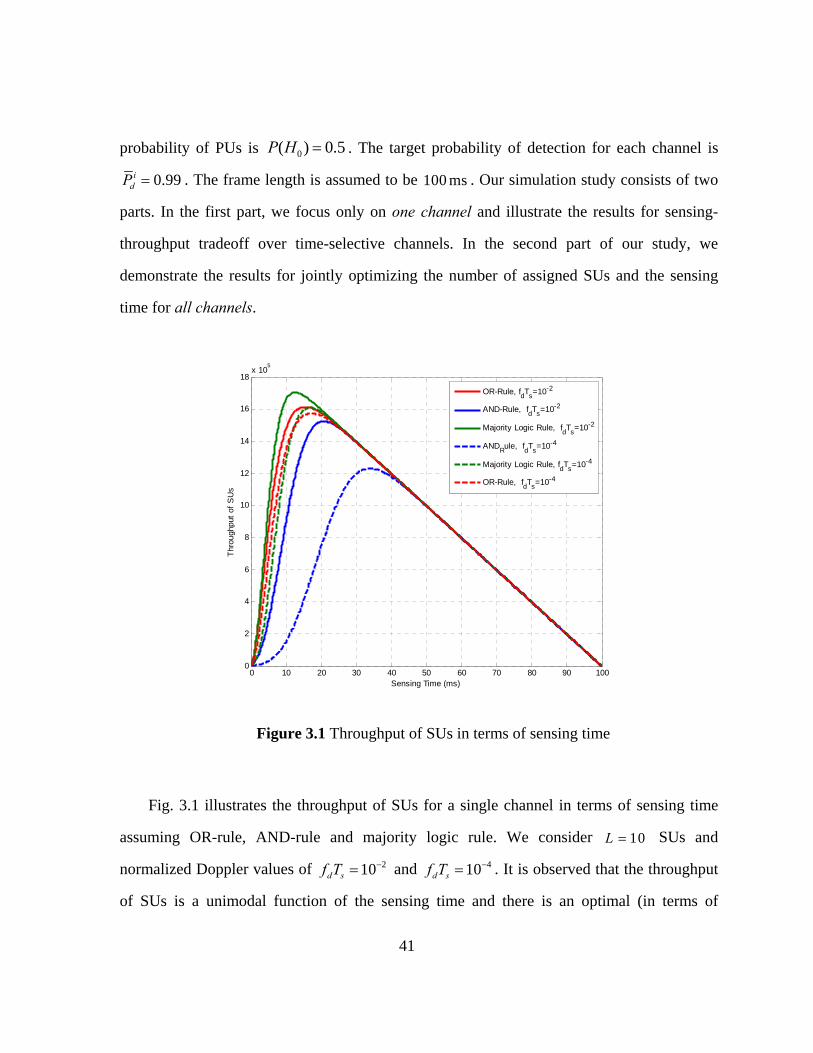
41
probability of PUs is 0( ) 0.5P H . The target probability of detection for each channel is
0.99idP . The frame length is assumed to be 100 ms . Our simulation study consists of two
parts. In the first part, we focus only on one channel and illustrate the results for sensing-
throughput tradeoff over time-selective channels. In the second part of our study, we
demonstrate the results for jointly optimizing the number of assigned SUs and the sensing
time for all channels.
Figure 3.1 Throughput of SUs in terms of sensing time
Fig. 3.1 illustrates the throughput of SUs for a single channel in terms of sensing time
assuming OR-rule, AND-rule and majority logic rule. We consider 10L SUs and
normalized Doppler values of 210d sf T and 410d sf T . It is observed that the throughput
of SUs is a unimodal function of the sensing time and there is an optimal (in terms of
0 10 20 30 40 50 60 70 80 90 1000
2
4
6
8
10
12
14
16
18x 10
5
Sensing Time (ms)
Thr
ough
put
of S
Us
OR-Rule, fdT
s=10-2
AND-Rule, fdT
s=10-2
Majority Logic Rule, fdT
s=10-2
ANDRule, f
dT
s=10-4
Majority Logic Rule, fdT
s=10-4
OR-Rule, fdT
s=10-4

42
throughput maximization) sensing duration which can be calculated from (3.17). It is further
observed that the optimal sensing time increases when the normalized Doppler value
decreases. The SUs need more time for sensing because the channel coefficients are more
correlated with decreasing Doppler value.
Figure 3.2 Throughput of SUs in terms of the number of SUs
Fig. 3.2 demonstrates the relationship between the throughput and the number of SUs
under the assumption that optimal sensing duration is used. In this simulation, we have
1 40L , 210d sf T and use (3.17) to optimize the sensing time. We observe that the
throughput increases with the increasing number of SUs as expected since the probability of
false alarm decreases.
0 5 10 15 20 25 30 35 401.1
1.2
1.3
1.4
1.5
1.6
1.7
1.8
1.9
2x 10
6
Number of SUs
Thr
ough
put
of S
Us
OR-Rule
AND-RuleMajority Logic Rule

43
Figure 3.3 Optimum sensing time of SUs over single channel in terms of SNR
In Fig. 3.3, we demonstrate the optimum sensing time versus the SNR of SUs. We
consider 10L SUs and normalized Doppler values of 210d sf T and 410d sf T . The
optimum sensing time decreases with the increasing SNR of SUs as a result of the
improvement in detection performance of SUs due to this SNR increase. With increase in
Doppler value, the channel coefficients are less dependent on each other and the detection
performance is improved, therefore there is less time required to maximize the throughput in
the same SNR. It can be also observed that OR-rule is more resistant to the channel
selectivity in comparison to the other two methods.
-20 -18 -16 -14 -12 -10 -8 -6 -4 -2 00
5
10
15
20
25
30
35
SNR(dB)
Opt
imal
Sen
sing
Tim
e (m
s)
OR-Rule, fdT
s=10-1
AND-Rule, fdT
s=10-1
Majority Logic Rule, fdT
s=10-1
AND-Rule, fdT
s=10-4
Majority Logic Rule, fdT
s=10-4
OR-Rule, fdT
s=10-4

44
In Fig. 3.4, we demonstrate the throughput of SUs versus the SNR of SUs over a single
channel. We consider 10L SUs and normalized Doppler values of 210d sf T and
410d sf T . The throughput of SUs increases with the increasing SNR of SUs similar to what
is observed for the sensing time in Fig.3.3. With increase in Doppler value, the channel
coefficients are less correlated and there is more temporal diversity available for the
detection of PUs. This therefore results in an increase in the throughput of SUs.
Figure 3.4 Optimum Throughput for SUs over single channel in terms of SNR
-20 -18 -16 -14 -12 -10 -8 -6 -4 -2 01.2
1.3
1.4
1.5
1.6
1.7
1.8
1.9
2x 10
6
SNR (dB)
Thr
ough
put
of S
Us
OR-Rule, fdT
s=10-1
AND-Rule, fdT
s=10-1
Majority Logic Rule, fdT
s=10-1
Majority Logic Rule, fdT
s=10-4
OR-Rule, fdT
s=10-4
AND-Rule, fdT
s=10-4

45
In the second part of our simulation, we assume a cognitive radio with 40 SUs and 10
channels. We jointly optimize the number of assigned SUs and the sensing time based on
(3.23) to maximize the total throughput of the network. In Fig. 3.5, we investigate the effect
of time selectivity on the throughput of SUs assuming majority logic rule. We demonstrate
the results for time varying Rayleigh fading channels with Doppler values of 110- , 210- ,
310- and further include the results for symbol-by-symbol independent Rayleigh fading
channel as a benchmark [48]. For 310d sf T , the channels coefficients are highly dependent
on each other. Among the Doppler values considered, the worst detection performance and
throughput of SUs is observed in this case. When the Doppler value increases to 210d sf T ,
the dependency of the channel coefficients decreases. This indicates a decrease in the
variance of decision statistic ( )iy , therefore the detection performance is improved in
comparison to 310d sf T . For 110d sf T , the channel coefficients are less correlated to
each other and it is observed that the throughput of SUs in this case converges to the
throughput of SUs over symbol-by-symbol independent Rayleigh channel.
In Fig 3.5, we have jointly optimized sensing time ( i ) and the number of SUs ( ik ) based
on (3.23). Now, in Fig. 3.6 we demonstrate that the joint optimization of these two variables
will indeed outperform when we optimize only one of the variables in each part and fix the
other one. We assume 210d sf T and consider the following two semi-optimal
benchmarking methods:
Method A (Fixed SU number and optimized sensing time): We assume that the
number of SUs for each channel is fixed and identical and only the sensing time is
optimized.
Method B (Fixed sensing time and optimized SU number): We assume a fixed
sensing time and optimize the number of SUs.

46
We observe that the joint optimization yields a throughput gain around 10% for some
SNRs in comparison with method A. In method A, each channel will be sensed by 4 SUs. For
Method B, we assume that sensing time occupies 25% and 10% of total time frame. It can be
seen that our proposed method outperforms Method B. We observe that the joint
optimization yields a throughput gain of around 15% and 25% related to method B which the
sensing time is 10% and 25% of total time frame, respectively.
Figure 3.5 Throughput of SUs over time varying channels with different Doppler values.
-25 -20 -15 -10 -50.4
0.6
0.8
1
1.2
1.4
1.6x 10
7
Mean SNR
Thr
ough
put
of S
Us
Rayleigh Fading Channel [10]
fdTs=10-1
fdT
s=10-2
fdTs=10-3

47
Figure 3.6 Throughput of SUs for the proposed method
-25 -20 -15 -10 -5 00.4
0.6
0.8
1
1.2
1.4
1.6x 10
7
Mean SNR
Thr
ough
put
of S
Us
Fixed K=4
Proposed MethodOptimum K, t=0.25 time frame
Optimum K, t=0.1 time frame

48
Chapter 4
Spectrum Trading for Concurrent Non-Identical Channel Allocation
in Cognitive Radio Networks
4.1 Introduction
In Chapter 2, we have proposed the spectrum trading using a multi-unit sequential sealed-
bid first-price auction for the shared used access model in cognitive radio. We have assumed
that the channels are non-identical and the value of each channel can be determined by the
channel capacity, data demand of SUs, and data transmission time. In sequential auction, the
channels are auctioned one after each other and each SU can submit one bid at the time,
while in concurrent auction the bidders submit their bids simultaneously for the channels.
Therefore concurrent auction needs less time and information overhead for holding auction
than the sequential auction. In this chapter, we aim to design a spectrum trading for non-
identical channel allocation using concurrent auction mechanism with exclusive usage
spectrum access model.
An important question faced by a licensee is how to allocate the spectrum rights to the
SUs in an optimal manner, i.e., to ensure maximum revenue for the PUs and maximum
satisfaction for SUs. Different SUs have different estimation about the value of available
channels. Since the license holder does not know the values that bidders attach to the
channels, auctions [7], [8], [25], [29], [56], [57], [68] provide an efficient mechanism for the
licensee to get higher revenue than that is obtainable via static pricing. Auctions are also

49
beneficial for the bidders, since, in general, they assign commodities to the bidders who
value them most.
In the current literature on spectrum auctions [7], [29], [56], [57], the valuation functions
used for the bidders are somehow unrealistic. In [56] and [25], Kasbekar et al. and Sengupta
et al. have considered a uniform distribution for the valuation function of the bidders.
However, in practical systems, the channel conditions and quality of service (QoS)
requirements of each user are different and therefore the channels have different and non-
identical values for SUs. In [68], a non-uniform valuation function has been proposed which
takes into account the channel capacity; however only one type of data traffic is considered
in this function ignoring the possibly different QoS requirements. In this chapter, we will
consider a realistic valuation function based on not only channel capacity, but also delay
sensitive and delay-insensitive data traffics of SUs.
Another common assumption in the current literature on spectrum auctions is that all
bidders are single-minded. It means that the bidders have non-zero valuation function for
only one bundle of channels. Moreover, the losers do not have the chance of revisiting the
remaining available channels. Such an assumption about bidders for non-identical channels is
not efficient, since the chance of winning for the bidders will decrease despite of the existing
unused channels for sale. From the auctioneer side, there are unused channels causing
inefficiency in channel utilization and, therefore, revenue degradation. To address this issue,
we consider r -minded bidders each of which can bid for r>1 bundles of channels in each
round of auction, but is allowed to win at most one of these bundles.
Another important issue that we want to address in this chapter is truthfulness1 or
incentive compatibility of combinatorial auction mechanism. To date, Vickrey-Clarke-Grove
1 If an auction mechanism has the property that each user should submit their true valuation if he/she wants to maximize his/her utility function, it is called truth-telling algorithm [59].

50
(VCG) mechanism is the only general method in which bidders should reveal their true
valuation to maximize their utility function or social welfare1 function. VCG mechanisms are
however required to compute the optimum outcomes of auction to be truthful. When there
are r -minded bidders with bid submission for more than one bundle of channels or when
there are single minded bidders with more than two channels in each bundle, the problem of
determining auction outcomes is NP-hard and there is not an optimum solution for these
cases. This problem should be solved by sub-optimal solutions therefore the VCG
mechanism is not truthful anymore. One of the open problems is to find sub-optimal
solutions which are truthful when the problem of determining auction outcomes is NP-hard.
In [59], Nissan et al. have proposed two VCG-based2 truthful sub-optimal solutions for
single-minded bidders using the so-called second chance mechanism. In [69], Lavi et al. have
introduced a sub-optimal solution for NP-hard VCG mechanism for single minded bidders
which is truthful in expectation3. In [70], Lehman et al. have demonstrated that there is a
simple truthful greedy algorithm for single-minded bidders and further proven that there is
not any payment scheme for the greedy algorithm with r -minded bidders to make it truthful
in general. To address this problem, we impose some restrictions for the bidders and propose
a weaker concept of truthfulness for r -minded bidders.
4.2 System Model and Problem Formulation
We consider a cognitive radio network with N SUs. Assume the availability of M (
N ) non-identical channels that the primary network wants to sell to the SUs. Let
1 2, , ..., NM be the set of all possible ways in which the M non-identical channels
1 The social welfare is the sum of utilities of all bidders for the specific channel allocation. 2 VCG-based mechanism is a mechanism that uses the suboptimal algorithm for determining the outcomes and calculates the payment of bidders based on VCG. 3 Truthfulness in expectation is a weaker concept than deterministic truthfulness [69].

51
can be allocated to N SUs. Let 1 2K , K ,..., Kj N , 1, 2,..., Nj M , denote a subset of
and each of its elements corresponds to a particular channel allocation. Therefore, each
element therein 1 2K , ,...,i mk k k , 1, 2,...,i N , represents the set of channels in the bundle
allocated to the thi bidder and m is the number of channels in a bundle.
We denote K( )i iV as the valuation function or utility of the thi SU for the channel
allocation K i j (i.e., the value that it conjectures or expects to derive from the allocation
when it submits the bids). Note that the valuation function of the thi SU is simply expressed
as i kV , 1 k M if the channel allocation K i consists of only one channel. The profit of
the thi SU is given by K K( , , ) ( )i i i i i i iu p V V p where ip is the payment that the thi SU
makes to the auctioneer for the channel allocation K i . Let (K )iiB denote the bid of the thi
SU for the channel allocation K i , i.e., the amount of money that the thi SU is willing to pay
if the allocation K i j is chosen. The auctioneer determines the channel allocation and the
payment ip .
The design of an auction can be formulated as an optimization problem to maximize
either revenue or social welfare. The social welfare [10] is the sum of the utilities of all
bidders from the allocation and therefore defined as 1(K )
N
i iiVSW . Furthermore, let *Ki
denote the channel allocation that maximizes the revenue of the auctioneer, given the bids
(.)iB , 1,…,i= N . That is, *Ki satisfies
*
1 1
(K ) (K ) K .N N
i i i i ii i
B B
(4.1)
For a truthful auction mechanism, the net utility of the thi bidder for any possible
bidding is maximized when it sets (K ) (K )i i i iB V , K i [58]. Therefore, in a truthful
auction mechanism such as VCG, since (.)iB is the announced valuation of bidders to the
auctioneer, *Ki obtained from (4.1) will also maximize the social welfare of the bidders. Let
52
*K j denote the allocation that would have maximized the social welfare if the thj bidder did
not participate in the auction. That is, *K j satisfies
* *
1, 1,
(K ) (K ) K .N N
i j i i ii i j i i j
B B
(4.2)
Under the VCG mechanism, the payment made by SU to the auctioneer is given by
* *
1, 1,
(K ) (K )N N
j i j i ii i j j i j
p B B
. (4.3)
The implementation of the VCG mechanism requires the calculation of *Ki and *K -j ,
1,...,j N . *Ki can be found by using a combinatorial optimization algorithm for the channel
allocation problem stated in (4.1), and *K -j can be found by running the same algorithm on
the set of bidders ignoring the thj bidder.
We consider two cases in which r -minded SUs can submit bid either only for single
channels or for bundles of channels. For case 1, let ,1 ,2 ,, , ...,i i i i Mb b bB be the bidding
vector (with r non-zero elements) of the thi bidder where ,i jb is its bid for the thj channel.
For case 2, let 1 1 1 1,1 ,2 ,, , ...,i i i i rb b b B be the r -tuple bidding vector of the thi bidder where 1
,i jb
denotes its bid for the thj bundle of channels. Furthermore, let , ,1 ,2 ,, ,...,i j i i i Ms s sS be an
M -tuple vector including the channels for which the thi bidder submits bid as its thj bid.
The SUs have their own valuation for the channels and this valuation mainly depends on
the capacity of the channel and traffic of SUs. The ergodic capacity of the thj channel for the
thi SU is given by [8]
2 2i, j j i, j i, j i, j i, jC = ln 1+G | h | P σ (4.4)
where j is the bandwidth of the thj channel and i, jP is the signal power of the thi SU in the
thj channel. In (4.4), i, jG and i, jh represent, respectively, the path loss and the fading
coefficient of the thj channel between the thi SU and Base Station. The fading coefficients

53
are modeled as complex Gaussian with zero mean and unit variance, leading to Rayleigh
fading model. The additive noise is modeled by a complex zero-mean Gaussian random
variable with a variance of 2i, jσ which follows a uniform distribution between min max
2 2σ ,σ
for each SU. Besides channel capacity, the valuation of a channel for SUs depends on their
data traffics. We assume that data packets arrive to the SUs following a Poisson distribution
with mean d for delay-sensitive traffic and o for delay-insensitive traffic ( d o ) [29].
In this case, r -minded bidders can bid for single channels. Based on the channel
capacity and traffic of SUs, we propose a valuation function for the single-item bidding as
1 2 , ,
1 , ,
,
if
( ) if
0 if
d o d oi i i k i i i k
d d d oi i i k i i k i i
di k i
Q D Q D C D D C
V k Q D C D C D D
C D
(4.5)
where diD and o
iD denote the required data rates of the SUs for transmitting , respectively,
delay-sensitive and delay-insensitive data traffic. We assume that data packets arrive to the
SUs following a Poisson distribution with mean d for delay-sensitive traffic and o for
delay-insensitive traffic ( d o ) [56]. Therefore, diD and o
iD are respectively functions of
d and o . Furthermore, let 1Q and 2Q 1 2Q Q denote the valuation coefficients of,
respectively, delay-sensitive and delay-insensitive data. 1 2Q Q shows that delay-sensitive
data has higher valuation than delay-insensitive data for the SUs. Based on this difference in
the valuation, the SUs should pay more to the auctioneer if they want to transmit delay-
sensitive data. We assume that two traffic types are independent from each other and also
independent from channel capacity.
In this case, the auctioneer asks bidders to submit at most r bids for the available single
channels, therefore each bidder submits an r -pair bid vector. As discussed above, we use
VCG as the auction mechanism. Since VCG is truthful when it is solved optimally, each user

54
should submit its true valuation to maximize its social welfare. If there are more than r non-
zero channel valuations for a bidder, the bidder submits the r most valuable channels to
maximize its valuation function since each bidder can submit only r bids.
Define the matrix 1 2; ; ...; NB B B B of size N M which contains all the biddings.
The thi row of this matrix represents the bidding of the thi bidder and the thj column
represents all the biddings for the thj channel. Let M NA denote an assignment matrix with
each of its element ,i ja being 0 or 1. If the thi bidder wins the thj channel, ,i ja is set to one,
otherwise zero. The channel allocation can be now stated as an optimization problem as
, ,1 1
, , ,1 1
arg max
s.t. i) 0,1 , ii) 0,1 , iii) 0,1
N M
i j i ji j
N M
i j i j i ji j
a b
a a a
A
. (4.6)
In the above, the second constraint means that the thj channel can be allocated to at
most one bidder. The third constraint indicates that each bidder can win at most one single
channel. This problem can be modeled as a bipartite maximum weighted matching
(BMWM)1 problem [71], [72] and be efficiently solved by sequential algorithms such as
Hungarian algorithm [73].
4.2.1 Case 2: r -minded bidders with bundle channel auction
In the previous sub-section, we have assumed that if the channel capacity is less than
SU’s delay-sensitive data traffic demand (i.e., ,d
i k iC D ), the bidder assigns zero value to the
channel. In this sub-section, we assume that bidders have the bundling capability of two or
more channels. Each of these channels is supposed to have lower capacity than the data
demand of bidders, but their aggregate capacities are equal or more than the demand. The
1 A weighted bipartite graph (or bi-graph) is a graph whose vertices can be divided into two disjoint sets such that every edge connects a vertex in one set to another set and the edges are weighted [71].
55
maximum number of the channels that can be bundled in a bid is denoted by m and is
determined by the auctioneer, (1 m M ).
The valuation function for a bundle of channels is given by
|K | |K |
1 2 , , ,1,2,..,|K |K 1 1
|K |
(K ) if max ( )i i
ii
i
d o d oi i i i i j i j i i i j
jj j
m
V Q D Q D C C D D C
(4.7)
where (K )i iV is the valuation of the thi bidder for the bundle of channels K i . Each bidder
can place r bids and each bid consists of at most m channels. The cardinality of K i is less
than or equal to m (i.e., | K |i m ).
In this case, bidders make their valuations for a single channel based on (4.5) and for a
bundle of channels on (4.7). As there is no budget constraint in our problem formulation, the
bidders can submit bids for m most valuable bids. Let K i, j denote the subset of the channels
as the thj bid of the thi bidder. The elements of ,i jS are given by
,,,
1if K
| K |
0 o.w
i ji ji j
js
(4.8)
where | K |i, j is the number of channels in the bid. For example if there are 5 channels for
sale and the first bidder wants to submit a bundled bid as its first bid consists of channels 1,2
and 4, the 1,1 1 3,1 3,0,1 3,0S . The matrix ,1 ,2 ,; ;... ;i i i i rS S S S of size r M
represents all channels that the thi bidder wants to submit bid for them. Let iA denote an M -
tuple assignment vector where each element ,i ja is either 0 or 1. When the thi bidder wins the
thj channel, ,i ja is set to one, otherwise zero. The channel allocation problem in case 2 can
be now formulated as

56
1
1
, 1 ,1
arg max )
s.t i) 0,1 , ii) 0,1 , iii) 0,1 , iv) 0,1
AA S (B
A S A S I
i
NT T
i i ii
NT T
i j i i i i r i ji
a a
. (4.9)
Here, the first constraint means that the thj channel can be allocated to at most one
bidder. The second constraint involves A STi i which is an r -tuple vector whose elements take
the value of either 0 or 1. It imposes that the thi bidder can only win the channels for which it
has submitted bidding. The third constraint 1 0,1Ti i rIA S checks that each bidder can only
win at most one bundle.
The problem in (4.9) is, in general, NP-hard and not solvable in polynomial time. There
have been some efforts in the literature for a solution in some special cases. Particularly, in
[58], for 1r , 2m , it was solved by maximum weighted matching in a graph. In [74], we
have considered 2r , 2m , modeled the problem as a 3-uniform hyper-graph1 and
proposed a greedy algorithm for finding a suboptimal channel allocation to the bidders. For
2r , 2m under consideration, the problem in (4.9) is NP-hard and can be modeled by
maximum weighted matching in hyper-graphs. This so-called “set packing” problem has
been studied in the context of combinatorial optimization and is one of the Karp’s NP-
complete problems [58].
Theorem 4.1: The allocation problem among r -minded bidders is NP-hard or the
decision problem of whether the optimal allocation has social welfare of at least q ( q is a
non-negative real number) is NP-complete
Proof: See Appendix C.
1 A hyper-graph is a generalization of a graph, where an edge can connect any number of vertices.

57
4.3 Sub-Optimal Solutions for Case 2
In the following subsections, we propose two approaches based on greedy algorithm
[70] and randomized rounding of LP relaxation algorithm [69] to find sub-optimal solutions
for our NP-hard problem. The prominent characteristics of these two approaches are good
approximation factor and being near-optimal despite of their computational simplicity.
4.3.1 Greedy Algorithm
Greedy algorithm [70] is a heuristic approach which involves finding the local optimum
at each stage which can be an approximation of the global optimum. Here, we propose a
simple greedy algorithm to find a sub-optimal solution for case 2 with an approximation
factor of max 1/ ,1/m M . We model our problem as a weighted hyper-graph and the
solution is to find the maximum weighted matching in this hyper-graph. A norm of a hyper-
edge ie is denoted by ( ) 1l
i i in e w v and is called “average bid per channel” for the thi
bid. Here, iw is the weight of thi hyper-edge which is equal to the amount of submitted bid
for K i , iv is the number of vertices of thi hyper-edge which is equal to | K | 1i , and l is a
constant factor ( 0l ).
Our proposed greedy algorithm selects the highest norm of hyper-edge in each step and
deletes all vertices inside the hyper-edge and other hyper-edges that have joint vertices with
the selected hyper-edge until there is not any non-zero hyper-edge left. The proposed greedy
algorithm steps can be then summarized as follows:
Step 1: Compute the norm of all hyper-edges and sort them in descending order. Then go
to step 2.
Step 2: Select the hyper-edge with the highest norm and allocate items inside this hyper-
edge to the bidder who placed this bid. Then go to step 3.

58
Step 3: Delete all hyper-edges that have any joint vertices with the selected hyper-edge in
the step 2. Delete all vertices belonging to the selected hyper-edge. Then go to step 4.
Step 4: If there is any hyper-edge with non-zero norm, go to step 2, otherwise end.
The proposed algorithm can be solved in ( log( ))O n n where n is the total number of
bids.
Theorem 4.2: The approximation factor of the proposed greedy algorithm with norm
1 2l is max 1/ ,1/m M .
Proof: See Appendix D
Since our auction mechanism is VCG-based, the payment of each winner bidder should
be calculated based on (4.3). The key part to calculate the payment of the th
j bidder (i.e., jp )
is to find *
1,(K )
N
i ij i jB
and *
1,(K )
N
i jj i jB . *Ki can be found via the greedy algorithm for
the channel allocation problem stated in (4.1), and *K -j can be found by running the same
algorithm on the set of the bidders ignoring the thj bidder. Therefore the payment of the th
j
bidder can be calculated as * *
1, 1,(K ) (K )
N N
i j i ij j i j j i jB Bp .
4.3.2 Randomized Rounding Relaxed LP (RRRLP) Algorithm
In the relaxed version of problem formulation in (4.9), each element of matrix A can be
in the interval [0,1] . Therefore we can reformulate (4.9) as
1
, 1 ,1
arg max
s.t i) 1, ii) 1, iii) 1, iv)0 1
i
NT T
i i ii
NT T
i j i i i i r i ji
a I a
AA S B
A S A S
. (4.10)
The re-formulated problem given by (4.10) is a LP problem that can be solved by
simplex method or interior points [75]. The output of the relaxed LP problem provides an
upper bound for the total social welfare and is not necessarily integral; therefore rounding the

59
fractional solution can be used to obtain an integral feasible solution. Different methods of
rounding have been proposed in the literature [75]. In this section, we will use randomized
rounding (RR). The basic idea of this method is to use the probabilistic method to convert an
optimal LP solution to a valid solution of the original problem. As the value of each
assignment is less than 1, a probability equal to this number can be assigned to each
fractional solution, i.e., if this value for the thj bid of the thi bidder is ,i ja , the channel will be
allocated to the thj bidder with the probability , ,( )i j i jP a a . Since in RR method, all
fractional solutions of (4.10) have the chance of rounding, this method is fairer related to the
bidders than the other rounding algorithms [69].
The steps of our proposed RRRLP can be therefore summarized as follows:
Step 1: Relax the integrality constraints in (4.9) and solve the relaxed LP version of the
problem in (4.10). Then go to step 2.
Step 2: Sort all the bids in decreasing order based on their fractional solution ,i ja . Then
go to step 3.
Step 3: Allocate the desired bundle to the bidder with the highest level in step 2 based on
the probability value that comes from the relaxed LP solution. Then go to step 4.
Step 4: Delete all the bids of winner bidder and all the bids that have joint item with the
allocated channel. Then go to step 5.
Step 5: If there is any non-zero bid or any channel is left, go to step 3. Otherwise end.
Because of randomized nature of this algorithm, it is possible that the integral solution of
this algorithm might be far from the LP fractional solution. However, based on the
probability distribution of this technique, the probability of being far from the optimal
solution is so small and it can be shown that the performance of this algorithm is near
optimal.

60
For the payment calculation of the RRRLP algorithm, similar to the greedy algorithm
discussed in the previous sub-section, first we need to find *Ki and *K -j . For the RRRLP
method, *Ki can be found by running the RRRLP algorithm to solve the outcome
determination problem of auction stated in (4.1), and *K -j can be found by running the same
algorithm on the set of bidders ignoring the thj bidder. Finally, jp can be calculated using
(4.3).
4.4 Truthful Iterated Greedy Algorithm for Case 2
The main challenge about VCG mechanism is that it should be calculated optimally to
be truthful. Since our problem is NP-hard for case 2, it cannot be optimally solved. In the
previous section, two sub-optimal methods have been proposed to solve this problem but
these methods ruin the truthfulness property of the VCG payment.
In [70], Lehman et al. have identified four properties for an auction mechanism to be
truthful. Based on these properties, they have designed a new truthful payment method for
single-minded bidders that satisfies these properties. They have further shown that there is
not any payment method to make an auction truthful for r -minded bidders [70]. To alleviate
this problem, we will use a weaker concept of truthfulness for bidders with some restrictions.
Particularly, we will consider myopic bidders1 and show that it is possible to design a truthful
auction for myopic complex bidders.
When the bidders are myopic, they cannot gain any information from the previous
rounds of auction. Such an assumption can be easily justified in our case: Since the bidders
are SUs and the items for sale are channels, we can assume that channel conditions (such as
noise, fading and interference) will change independently in each round of auction.
Therefore, bidders are not able to use the information from previous rounds. Furthermore, we
1 A bidder who disregards future auctions in a sequential setting is called myopic bidder.

61
assume that traffic of SUs will change independently from one round to another round;
therefore SUs do not have any estimation about the demand of other SUs.
The complexity of the algorithms for determining auction outcomes can be decreased
through the employment of some iterative techniques. Another advantage for iterative
outcome determination algorithm is that our problem can be reduced from r -minded bidders
to single minded bidders. In [76], it has been shown that if the output of an iterative auction
is computed optimally in each iteration, it will be truthful. On the other hand, if the outcome
determination will be greedy in each iteration but satisfies monotonicity and participation
property it will be truthful for myopic bidders [70].
Definition: An outcome determination algorithm has monotonicity property if a bidder
i is granted a bundle with bid K i , it is also granted each bundle K Ki i with norm i in n .
Participation property ensures that the bidder will not lose by participating in the
auction. It indicates that the winning bidder’s payment should not be more than its submitted
bid. In our outcome determination algorithm, the bids of all bidders are sorted based on their
average bid per item or norm of each bid. In each iteration of the algorithm, a most valuable
bid of each bidder is selected for use in the current iteration. After each iteration, all bids
used in this iteration, all bids of winning bidders, and all bids that have joint item with the
winning bids are deleted. Iterations continue until there is no item or no bid left. The steps of
our proposed truthful iterated greedy algorithm can be therefore summarized as follows:
Step 1: Sort r bids of each bidder based on their norms in descending order.
Then go to step 2.
Step 2: Pick the most valuable bid of each bidder. Then go to step 3.
Step 3: Apply the proposed greedy algorithm in sub-section 4.3.1 and determine the
winning bidders. Then go to step 4.

62
Step 4: Payment of each bidder should be determined based on the employed payment
method (See below for further discussions) Then go to step 5.
Step 5: Delete all the bids of winner bidder and all bids of other bidders that have joint
items with the winner bid. If there is any channel or any bid left, go to step 2, else end.
For the payment, we use a modified version of the payment method in [70]. In this
method, we find the most valuable bid that has at least one joint item with the winning bids.
Let ( )Ln j denote this bid. If the number of items in winning bid is | K |j , the winning bidder
should pay | K | ( )j Ln j . In the original payment method of [70], all bids are considered in
payment determination. In our modified version, the payment of each bidder will be
determined by the participant bids in each iteration, not all bids. Therefore, the payment of
each bidder is affected by at most one bid of other bidders used in each iteration. With this
method of payment and under the assumption of myopic bidders, we can model r -minded
bidders as single minded bidders.
Proposition: The proposed iterated greedy algorithm for the myopic bidders is truthful.
Proof: The proposed modified payment method guarantees that the payment of the
bidders is always less than the submitted bid. In our proposed iterated greedy method, the
winners in each iteration will be determined based on the most valuable bids with the highest
norms. For the payment calculation of the winner bidder in each iteration, first we find the
most valuable bid that has at least one joint item with the winning bid of bidder in the same
iteration. It is clear that the selected bid (which has joint item with the winning bid) has less
norm than the norm of winning bid; otherwise, this bid should have been selected as the
winning bid. Therefore, we can conclude that our proposed payment method satisfies the
participation property.
Based on the monotonicity definition, an outcome determination algorithm has the
monotonicity property if a bidder i is granted a bundle with the bid K i and the norm in , it

63
will be granted each bundle K Ki i with the norm i in n . Therefore for the monotonicity
proof, it is sufficient to show that if this bidder submits bundle K i (i.e., K Ki i ) with
i in n instead of the bundle K i , it should also win bundle K i . The greedy algorithm works
based on the highest norms. The bidder i was winner with norm in for the bundle K i ,
therefore it means that the bundle K i with norm in was among optimal bids with the highest
norms. If the bidder i submits a bid for bundle K i with norm in , since its norm in is bigger
or equal than in , therefore we can conclude that in is among optimal bids with the highest
norms and also it has no conflicts with bids with higher norms since the bidder i was winner
with the bid K i . Therefore the bidder i is also the winner for the bundle K i . Since the
iterated greedy algorithm satisfies the monotonicity and the participation property for the
myopic bidders, the proposed algorithm is truthful.
In addition to the truthfulness property, there are two advantages of our proposed
algorithm in comparison with the VCG auction. First, the complexity of our problem is less
than that of VCG mechanism. Second, when the VCG mechanism is solved by a sub-optimal
algorithm, rationality of the bidders may not be satisfied but in our proposed algorithm, the
payment of the bidders are always less than the bidders submission and therefore their
rationality are satisfied.
4.5 Simulation Results
In this section, we provide Monte-Carlo simulation results to demonstrate the
effectiveness of the proposed auction framework and compare it with previous methods [57],
[68] in terms of total social welfare, revenue of the auctioneer, and profit of bidders. In our
simulations, we use the notation of “currency unit (CU)” instead of any particular currency.

64
We assume that all channels have a bandwidth of 6 MHz. For data traffic of SUs, we assume
1o Mbps and 0.5d Mbps.
In Fig. 4.1, we illustrate the average auctioneer revenue versus the number of bids r for
case 1. We assume that the number of channels is M =10 and the number of bidders are
11 16N£ £ . We see that the average revenue increases when the number of bids increases.
This indicates that the efficiency of the spectrum utilization is better for 1r , because there
is not any unused channel. It is also observed that the auctioneer’s revenue saturates for
7r . On the other hand, the overhead information caused by bidder’s submissions increases
with the increasing number of submitted bids. Therefore we can prevent the increase in
overhead information by fixing r at the saturation point which is 7r = in our simulation. It
is also observed from Fig. 4.1 that the auctioneer’s revenue increases as the number of
bidders increases from 11 to 16. This increase is a result of the increasing competition
between bidders and increasing in amount of their bids. Since the outcome determination of
auction is optimum in case 1, the auction mechanism in case 1 is truthful.

65
Figure 4.1 Average revenue of the auctioneer in case 1, i.e., the SUs are r -minded but they
can submit bid only for single channels.
In Fig. 4.2, we illustrate the average auctioneer revenue versus the number of bids r
for case 2 and compare the performance of proposed greedy, RRRLP and truthful greedy
algorithms (See Section 4.3 and 4.4). We assume that the number of channels is M =10 and
the number of bidders is N = 19. As discussed in Section 4.4, the RLP algorithm provides an
upper bound for the revenue of auctioneer and is included here as a benchmark. We further
include the performance of the greedy algorithm proposed in [70] as a competing scheme. It
can be observed that the RRRLP method outperforms greedy and truthful greedy method in
1 2 3 4 5 6 7 8 9 10500
1000
1500
2000
2500
3000
Number of Bids
Ave
rage
Rev
enue
for
the
Auc
tione
er
Average revenue for the auctioneer in terms of number of bids in case 1
N=11
N=12
N=13N=14
N=15
N=16

66
terms of auctioneer’s revenue. The performance of our RRRLP and greedy algorithms are
also better than the greedy algorithm in [70]. It can be also observed that the greedy
algorithm in [70] outperforms the truthful greedy algorithm in terms of auctioneer revenue.
Specifically, the approximation factors for the RRRLP, the greedy algorithm, the truthful
greedy algorithm are 75%, 65% and 30%, respectively, while the approximation factor for
the greedy algorithm in [70] is 55%.
Figure 4.2 Average revenue of auctioneer in case 2, i.e., the SUs are r -minded and they can
submit bid for bundles of channels.
1 2 3 4 5 6 7 8 9 10500
1000
1500
2000
2500
3000
3500
Number of BidsNumber of bidders = 19
Ave
rage
Rev
enue
for
the
Auc
tione
er
Average revenue for the Auctioneer in terms of number of bids in case 2
Greedy Truthful
Greedy in [70]
RLPGreedy
RRRLP

67
In Fig. 4.3, we illustrate the total social welfare for case 2. We assume that the number
of channels is M =10 and the number of bidders are N = 19. Similar to Fig. 4.2, RLP
provides an upper bound on the performance of methods under consideration. RRRLP
performs the best followed by the proposed greedy algorithm, greedy algorithm in [70] and
the proposed truthful iterated greedy algorithm.
Figure 4.3 Average total social welfare in case 2.
In Fig. 4.4, we provide the average profit of bidders in case 1. It can be observed when
the number of bidders are 11, 12, 13, SUs have profit improvement in parallel to the increase
in r , since all the channels are not fully utilized. The profit of the SUs saturates when r is
1 2 3 4 5 6 7 8 9 102200
2400
2600
2800
3000
3200
3400
3600
3800
4000
4200
Number of BidsNumber of bidders = 19
Ave
rage
tot
al s
ocia
l wel
fare
Average total social welfare in terms of number of bids in case 2
Greedy in [70]
Greedy
RRRLPRLP
Truthful Greedy

68
close to the number of channels, i.e., 10 in our simulation. When the number of bidders are
14, 15 and 16, the average profit of bidders degrades in parallel to the increase in r .
Because, the spectrum is fully utilized therefore with increasing r , the payment of bidders
increases due to more competitors for each channel and the profit of them (that is the
difference between valuation and payment) decreases.
Figure 4.4 Average revenue of bidders in case 1.
In Fig. 4.5, we provide the average profit of bidders in case 2. We assume that the
number of channels is M =10 and the number of bidders are N = 19. Similar to case 1, the
1 2 3 4 5 6 7 8 9 1020
30
40
50
60
70
80
90
100
110
Number of Bids
Ave
rage
Pro
fit o
f B
idde
rs
N=16N=15
N=14
N=12
N=13N=11

69
average profit of bidders degrades with the increase of number of bids. We also observe that
the truthful greedy algorithm outperforms RRRLP and greedy algorithms in terms of profit
for the bidders. Since in truthful greedy algorithm, bidders submit their true valuation to
maximize their profit, the bidder gains more revenue than two other methods. It should be
also noted that the complexity of truthful iterated greedy algorithm is less than greedy and
RRRLP algorithm.
Figure 4.5 Average revenue of bidders in case 2.
1 2 3 4 5 6 7 8 9 1020
40
60
80
100
120
140
160
Number of BidsNumber of bidders = 19
Ave
rage
Rev
enue
for
the
bid
ders
Average revenue for the bidders in terms of number of bids in case 2
Truthful Greedy
RRRLPGreedy
Greedy in [70]

70
Chapter 5
Pricing for Open Access Oligopoly-Market Femtocell Networks
5.1 Introduction
The current market in femtocell networks is mainly geared towards close access (CA)
femtocells [60]. To enable the wide deployment of open access (OA) femtocells, innovative
pricing models with incentives for residential femtocell users are required that will be
pursued in this chapter. In [30], Shetty at al. study the impacts of user incentives on the
revenue of a femtocell operator in CA model. In [61], the economic aspects of openness of
femtocells compared with close femtocells is studied. This paper considered the monopoly
market which is the simplest market structure when there is only one seller in the system.
Some papers [5], [61] propose fixed pricing strategy for open access femtocells, but fixed
pricing has some drawbacks such as the lack of economic incentives for femtocells and
revenue degradation for mobile service provider. In [77], Duan et al. investigate the
economic incentive for the cellular operator to add femtocell service on the top of its existing
macrocell service. They model the interaction between cellular operator in a monopoly
market and users as a Stackelberg game. They showed that the operator choose to only
provide femtocell service if femtocell service has full spatial coverage. In [32], VCG auction
is proposed as the pricing scheme for open access femtocells. In [33], a reverse auction (one-
buyer-multiple-sellers) framework is proposed based on VCG mechanism for access
permission trading between wireless service provider and private femtocell owners.
In our work, we assume oligopoly market [8] where there exist multiple sellers and
multiple buyers. The sellers compete with each other independently to achieve the highest
revenue by controlling the quantity or the price of the supplied commodity. The oligopoly
market is more realistic to use in femtocell networks because there are different mobile

71
service providers in practice. The providers should involve residential customers to share
their spectrum by innovative policies in pricing and QoS warranties. In this regard,
interaction of users and mobile service providers play a vital role in the OA femtocell
networks. From the user point of view, CA is obviously preferred by residential customers
who will have full control over the list of authorized users. However, some surveys indicate
that OA might be an attractive business model for home market conditioned that competitive
pricing is offered [4], [78]. Hybrid access (HA) methods are also discussed to reach a
compromise between the impact on the performance of subscribers and the level of access
that is granted to non-subscribers [78]. Therefore, the sharing of femtocell resources between
subscribers and non-subscribers needs to be finely tuned. Otherwise, subscribers might feel
that they are paying for a service that is to be exploited by others. The impact to subscribers
must thus be minimized in terms of performance or via economic incentives. With a proper
pricing model, deploying of an OA or HA model is more beneficial for network operators
than CA model by providing an inexpensive way to expand their network capacities by
leveraging third-party backhaul for free.
5.2 System Model and Problem Formulation
Consider a wireless cellular network consisting of N macro base stations (MBSs) and
several femtocell access points (FAP). The macro user equipments (MUEs) are served by N
MBSs from different mobile service providers. In the literature, Homogenous Spatial Poisson
Process (HSPP) is widely used to statistically model the locations of FAPs and MUEs [79].
In our work, we consider Clustered Spatial Poisson Process (CSPP) for FAPs and MUEs
(See Fig.5.1.a) which is more realistic in practical scenarios. In Fig.5.1, the blue points are
FAPs and the green points are MUEs. In Fig.5.1.a, the FAPs with CSPP distribution form a

72
cluster represented by the red circle. It is assumed that the FAPs inside each cluster can be
controlled by a controller.
a. Clustered Spatial Poisson Process (CSPP)
b. Homogenous Spatial Poisson Process (HSPP)
Figure 5.1 Geographical distribution of FAPs under HSPP and CSPP assumptions.
In CSPP model, we have some clusters of femtocells in macrocell layer with HSPP
distribution and there is a random number of femtocells distributed identically within each
cluster area. This assumption is particularly realistic for urban residential areas in which
several FAPs exist clustered in apartment buildings. Denote 2H RÌ as the interior of a
reference hexagonal macrocell C of radius CR . The cellular users (i.e., MUEs) are distributed
on 2R according to a CSPP CW of intensity Cl . On the other hand, locations of FAPs are
assumed to form a CSPP fW with intensity fl . Each femtocell includes a Poisson distributed
population of actively transmitting femtocell user equipments (FUEs) with mean fU in a
circular coverage area of radius fR , f CR R [79].
Since the distribution of FAPs follows CSPP, they can be grouped for cooperation in a
macrocell layer and the available channels can be divided among FAPs of each group. The
-500 -400 -300 -200 -100 0 100 200 300 400 500
-400
-300
-200
-100
0
100
200
300
400
Clustered Spatial Poisson Process (CSPP)
-500 -400 -300 -200 -100 0 100 200 300 400 500
-400
-300
-200
-100
0
100
200
300
400
Homogenous Spatial Poisson Process (HSPP

73
same channels can be used by another group of the FAPs in a macrocell with far enough
distances between each other. Consider a two-tier LTE system and assume that FAPs can be
grouped with respect to their intra-channel coefficients and geographical location to each
other (i.e., FAPs with high channel gain between each other and distances less than a certain
threshold can be categorized in the same group). Resource allocation, scheduling and other
signaling of FAPs with MBSs can be carried out via the controller. We also assume that
MBS’s antenna is sectorized, therefore the available channels for FAPs in each sector would
be different from those in other sectors (See Fig.5.2).
Figure 5.2 Cellular network underlaid with femtocell network
To determine the available channels, we assume that FAPs are equipped with spectrum
sensing ability and perform cooperative sensing. This method avoids the overhead required
for periodical MBS announcements if spectrum sensing is carried out by MBSs. Therefore

74
FAPs find their suitable channels based on their requirements and send their requests to the
controller of group. The controller collects and sends their request to the MBSs.
5.3 Pricing Schemes
In our work, we assume OA model in which any user can access to any femtocell. The
use of OA FAPs at home in fact reduces the interference problems caused by CA FAPs.
Indeed, all nearby users would be authorized to connect to any femtocell, reducing thus the
negative impact of the femtocell tier on the macrocell network. In this case, the MUEs are
always connected to the strongest server (either macrocell or femtocell), avoiding cross-tier
interference. As a result, the overall throughput of the network increases. OA is therefore
advantageous from the operator point of view.
In OA femtocell networks, the unit price of spectrum should be determined dynamically
because of different demand and supply from femtocell and macrocell sides. In this case, the
femtocell users have good incentives to participate in OA model and the service providers
can maximize their revenue. In previous works [61], fixed pricing is suggested for OA that is
not desirable by residential users and they do not have any tendency to use this model.
As we mentioned in the first chapter, the design of the pricing model can be considered
as a spectrum trading problem and microeconomics and game theory provide a set of
powerful mathematical tools for the analysis of spectrum trading problem. In the following
sub-sections, we propose pricing models for OA femtocells based on market equilibrium,
Bertrand game, multiple leader multiple follower Stackelberg game and Cooperative game.
5.3.1 Market Equilibrium
In market equilibrium approach used in microeconomics, the profit of the seller and the
satisfaction of the buyer(s) are maximized. The amount of commodity that the seller is

75
willing to supply to the market is indicated by a supply function. The supplied quantity is a
function of price p and denoted by ( )S p [8]. On the buyer side, the amount of commodity
that the buyer is willing to buy from the market is defined by a demand function denoted by
( )D p . In general, the amount of supply from the seller is an increasing function of price
while the demand for a commodity in the market is a decreasing function of price. Given the
demand and supply functions in a market, the market-equilibrium price is given by the price
for which the supply equals the demand, i.e., ( ) ( )S p D p= .
In our case, the negotiation on price and the size of allocated spectrum between the
FAPs and MBS is performed through a controller (it could be a server which has control
interfaces to both MBSs and FAPs). We categorize FAPs in groups with respect to their
channel gains and geographical locations. All FAPs of a specific group submit their spectrum
requirements to the controller. The controller checks the spectrum availability and unifies all
demands into one demand and submits them to MBSs. MBS determines the price for per unit
of spectrum based on its supply function and returns this price to the controller. Then the
controller allocates demanded spectrum to each FAP. We assume that the maximum demand
of a FAP is limited and each FAP can access to a limited number of channels. Furthermore, it
is assumed that the sum of demands of FAPs for spectrum is less than a fraction of the
available spectrum because MBS should also serve other MUEs that request services but not
serviced by the FAPs. Spectrum demand of FAPs can be determined using their utility
function. The utility function of all FAPs can defined as [80].
2
1 1
1( (1 ) 2
2
N N
i i i i i i i i i i i i ji i i j
u C Ab C b p C d p b b v b b= = ¹
é ùê ú- + - - +ê úë û
å å åb) = (5.1)
where b is the vector of shared spectrum from all MBSs with FAPs, i.e., [ ]1 2, , ..., Nb b bb = ,
N is the number of MBSs, and iC is the fraction of spectrum that is used for FUEs. The

76
reason for the power 2 for ib in (5.1) is that it makes the utility function concave. (1 )iC- is
the fraction of spectrum that is used for MUEs. ip is the unit price for spectrum from thi
MBS. iA is the spectral efficiency for FUEs served by FAPs and is a function of signal-to-
noise ratio (SNR) and targeted error rate performance. MBS pays to FAPs i id p (as the unit
price of spectrum for serving of MUEs by FAPs) where id is a fixed coefficient and
0 1v£ £ is another coefficient [81] which shows the substitutability. Specifically, if 0v = ,
the FAPs cannot switch among frequency spectra, while if 1v = , the FAPs can switch
among frequency spectra freely.
The demand function for spectrum which belongs to the thi MBS can be calculated by
( )(1 ) , {1,2,..., }i i i i i i i i j
j ii
UC A C p C d p b v b i N
b ¹
¶= - + - - - Î
¶ åb
. (5.2)
Solving this linear system with N equations, we find
( )( ) ( )( )
( )
( )( )( )( )
1 2( ) (1 )
1 1 1
(1 )1 1 1
i i i i i i i i
j j j j j j jj i
N vD C A C p C d p
v N v
vC A C p C d p
N v v¹
+ -= - + -
- + -
- - + -+ - -å
p
. (5.3)
This shows the optimum amount of spectrum that MBSs want to sell with price vector p .
The demand function for the thi service provider can be separated in two parts; one part that
is dependent on ip and the other part that is dependent on the price of others [... ... ]i jp- =p ,
j i¹ . The demand function can be therefore written as
( )i i i j j ij i
D X p Y p l¹
= + +åp (5.4)
where iX , jY and il are some constant coefficients. The revenue of the thi MBS from selling
spectrum to the FAPs can be calculated by [22]
( )( )2
( ) (1 ) ( ) (1 )i i i i i i i i i i i i i i i i i iR p C p b C d p b M w b k C b k M w bé ù= - - + - + - - - -ë û (5.5)

77
where iw is the total spectrum available for the thi MBS to be allocated to the MUEs and
FAPs. Power coefficient in the last term of (5.5) makes the utility function concave. iM ,
1, 2,...,i N= are the spectral efficiencies of MUEs served by the thi MBS. ik is the spectral
efficiency for MUEs inside the group area served by FAPs. (1 )i i iC b k- is the revenue of
MBSs from MUEs which are serviced by the FAPs. i i iC p b is the payment of FAPs to the
MBSs based on their usage from spectrums. (1 )i i i iC d p b- is the amount of discounts that
MBSs should give to the FAPs for providing services to MUEs. Since the spectrum
efficiency for the MUEs served by FAPs is more than that of MUEs served by MBS
( i ik M> ) therefore the term ( )( )2
i i i ik M w bé ù- -ë û represents the performance degradation of
MUEs users served by MBS. The supply function can be calculated from
( )( ) ( )2
(1 ) (1 ) 2 0ii i i i i i i i i i i i
i
RC p C d p M k C k M w b
b
¶= - - - + - - - - =
¶p
. (5.6)
By solving (5.6), ( )iS p can be calculated as
( )( )
2
2
(1 ) (1 ) 2( )
2i i i i i i i i i i i
i
i i
C p C d p M k C k M wS
k M
- - - + - - -=
-p . (5.7)
The supply function for the thi service provider can be separated in two parts; one part
that is dependent on ip and the other part is a constant. Therefore it can be rewritten as
( )i i i iS V p q= +p (5.8)
where is and iq are constant coefficients. The market-equilibrium solution will be then
defined as the price *ip at which spectrum supply equals spectrum demand given by
* *( ) ( )i iS D=p p . To calculate the prices for the market equilibrium, we should solve
following set of linear equation system using (5.4) and (5.8), i.e,
, , {1,2,..., }i i j j i i i ij i
X p Y p l V p q i j N¹
+ + = + Îå . (5.9)
*ip can be calculated as (See Appendix E)
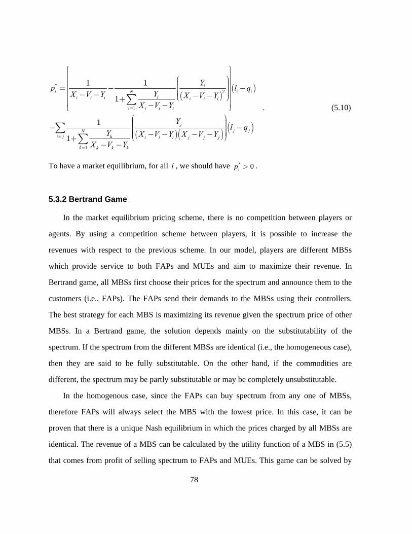
78
( )( )
( )( ) ( )
*2
1
1
1 1
1
1
1
ii i iN
ii i i i i i
i i i i
jj jN
i j k i i i j j j
k k k k
Yp l q
YX V Y X V YX V Y
Yl q
Y X V Y X V YX V Y
=
¹
=
é ùê úæ öê ú÷ç ÷çê ú= - -÷ç ÷ê úç- - ÷ç - -è øê ú+ê ú- -ë û
æ ö÷ç ÷ç- -÷ç ÷ç ÷- - - - ÷çè ø+- -
å
åå
. (5.10)
To have a market equilibrium, for all i , we should have * 0ip > .
5.3.2 Bertrand Game
In the market equilibrium pricing scheme, there is no competition between players or
agents. By using a competition scheme between players, it is possible to increase the
revenues with respect to the previous scheme. In our model, players are different MBSs
which provide service to both FAPs and MUEs and aim to maximize their revenue. In
Bertrand game, all MBSs first choose their prices for the spectrum and announce them to the
customers (i.e., FAPs). The FAPs send their demands to the MBSs using their controllers.
The best strategy for each MBS is maximizing its revenue given the spectrum price of other
MBSs. In a Bertrand game, the solution depends mainly on the substitutability of the
spectrum. If the spectrum from the different MBSs are identical (i.e., the homogeneous case),
then they are said to be fully substitutable. On the other hand, if the commodities are
different, the spectrum may be partly substitutable or may be completely unsubstitutable.
In the homogenous case, since the FAPs can buy spectrum from any one of MBSs,
therefore FAPs will always select the MBS with the lowest price. In this case, it can be
proven that there is a unique Nash equilibrium in which the prices charged by all MBSs are
identical. The revenue of a MBS can be calculated by the utility function of a MBS in (5.5)
that comes from profit of selling spectrum to FAPs and MUEs. This game can be solved by

79
Nash equilibrium using the best response function. The best response function of the thi MBS
given the spectrum price of other MBSs is defined as
( ) arg max ( , )i
i i i i ip
B R p- =p p . (5.11)
The Nash equilibrium of this game is denoted by the vector * *[... ...]ip=p where
* *( )i i ip B= p . *ip is the vector of the best response of other player except i . For calculation
of the Nash equilibrium, we should solve the set of equations 0i iR p¶ ¶ = for all i . The size
of shared bandwidth in (5.5) is replaced by the demand of femtocells ( )iD p . The revenue
function of thi MBS can defined as
( )( )2
( ) ( ) (1 ) ( )
( ( )) (1 ) ( ) ( )
i i i i i i i i
i i i i i i i i i i
R C p D C d p D
M w D k C D k M w D
= - -
é ù+ - + - - - -ë û
p p p
p p p . (5.12)
Solving 0i iR p¶ ¶ = yields the Nash equilibrium. The Nash equilibrium can be achieved by
solving following linear equations:
( )
[ ] ( )2
( (1 ) ) ( )
( (1 ) ) (1 ) 2 ( )
ii i i i
i
i i i i i i i i i i i i
RC C d D
p
C C d p k C M X k M X D
¶= - -
+ - - + - - + -
pp
p
(5.13)
(5.13) can be rewritten as
{ }0, , 1,2,...,i i j j ii j
A p Z p e i j N¹
+ + = Îå (5.14)
where iA , jZ and ie are respectively given by
( )2 22( (1 ) ) 2i i i i i i i iA C C d X k M X= - - + - . (5.15)
( )( )2( (1 ) ) 2j i i i i i i j
i j
Z C C d k M X Y¹
= - - + -å . (5.16)
( )( ) ( )2( (1 ) ) 2 (1 )i i i i i i i i i i i ie C C d k M X l k C M X= - - + - + - - . (5.17)
Since there are N service providers, we have N linear equations to solve and calculate ip ,
{ }1, 2,...,i NÎ . Based on the lemma in the Appendix E, we can solve (5.14) as

80
( )( )
( )( ) ( )2
1 1
1 1 1
1 1
jii i jN N
i ji ii i i i j ji i
i ii i i i
ZZp e e
Z ZA Z X Z X ZX ZA Z A Z
¹
= =
é ùê ú æ öæ öê ú ÷÷ çç ÷÷ ççê ú= - - ÷÷ çç ÷÷ê ú çç- ÷÷ - -ç ÷- çè ø è øê ú+ +ê ú- -ë û
åå å
.(5.18)
To have Nash equilibrium for the bargaining game for all i , we should have 0ip > .
5.3.3 Multiple Leader Multiple Follower Stackelberg Game
In multiple leader multiple follower (MLMF) Stackelberg game, there are some service
providers (called as “leaders”) who enter the market sooner than the other service providers,
therefore they determine the prices of spectrum sooner than the others. Therefore the other
service providers (called as “followers”) should determine their prices after the leaders
determine the price of spectrum. In the Stackelberg game, since the leaders will make the
decision before the followers, the followers will choose their optimal strategy based on the
observed strategy chosen by the leader. Consequently, the solution of this game is a set of
strategies where the profit of the leader is maximized and the followers choose their best
responses.
In a Stackelberg game, the solution which maximizes the profit of the leader is defined
as the Stackelberg equilibrium. The Stackelberg equilibrium can be obtained by backward
induction. In backward induction, the best response of the follower is first obtained. Then,
from this best response of the follower, the leader optimizes its strategy to achieve the
highest profit. We assume that there are I leaders and N I- followers in the system. In our
case, MBSs { }1, 2,...,i N I= - are followers and MBSs { }1,...,i N I N= - + are leaders.
Based on the backward induction, first we should calculate the price of followers in terms of
price of leaders. Mathematically speaking, we need to calculate 0i iR p¶ ¶ = for

81
{ }1, 2, ...,i N I= - and calculate [ ]1 2, , ..., N Ip p p - in terms of the price of leaders, i.e.,
1, ...,N I Np p- +é ùë û . Then we can calculate price of leaders by 0i iR p¶ ¶ = for
{ }1,...,i N I N= - + . Therefore, based on the Stackelberg equilibrium, leaders will have
more flexibility to determine the price of spectrum and therefore will gain more revenue than
the followers.
To calculate price of followers in terms of price of leaders, first we should use (5.11) to
calculate price of service providers{ }1, ...,I N+ . Therefore if we use same method in the
previous sub-section, the linear equations for calculating price of followers are given by
{ } { }1
0, 1,2,..., , , 1, 2,...,I
i i j j i k ki j k
A p Z p e Z p k I i j I I N¹ =
+ + + = Î Î + +å å (5.19)
where iA , jZ and ie are respectively given by
( )2 22( (1 ) ) 2i i i i i i i iA C C d X k M X= - - + - . (5.20)
( )( )2( (1 ) ) 2j i i i i i i j
i j
Z C C d k M X Y¹
= - - + -å . (5.21)
( )( ) ( )2( (1 ) ) 2 (1 )i i i i i i i i i i i ie C C d k M X l k C M X= - - + - + - - . (5.22)
In (5.19), kp , {1,..., }k IÎ are the price of leaders and considered to be constant
coefficients. Therefore, the price of followers in terms of the price of leaders can be
calculated as
( )
( )( )
21
1
1
1
1 1
1
1 , { 1,..., }
1
Ii
i i k kNkii i i i
i i i
Ij
j k kNi j ki i i j j
i i i
Zp e Z p
ZA Z X ZA Z
Ze Z p i I N
Z X Z X ZA Z
=
=
¹ =
=
é ùê úæ ö æ öê ú÷ç ÷ç÷çê ú= - + ÷÷ çç ÷÷ ç ÷ê úç- è ø÷ç -è øê ú+ê ú-ë û
æ öæ ö÷ç ÷÷çç- + Î +÷÷çç ÷÷ç ÷ç ÷è ø- - ÷çè ø+-
åå
å åå
(5.23)
We can rewrite the price of followers as

82
1
, { 1,..., }, {1,2,..., }I
i i k kk
p e Z p i I N k I=
¢ ¢= + Î + Îå (5.24)
where ie¢ and iZ ¢ are respectively given by
( )
( )( )
2
1
1
1 1
1
1
1
ii iN
ii i i i
i i i
jiN
i j i i i j j
i i i
Ze e
ZA Z X ZA Z
Ze
Z X Z X ZA Z
=
¹
=
é ùê úæ öê ú÷ç ÷ç¢ ê ú= - ÷ç ÷ê úç- ÷ç -è øê ú+ê ú-ë û
æ ö÷ç ÷ç- ÷ç ÷ç ÷- - ÷çè ø+-
å
åå
(5.25)
( )
( )( )
2
1
1
1 1
1
1
1
ii iN
ii i i i
i i i
jiN
i j i i i j j
i i i
ZZ Z
ZA Z X ZA Z
ZZ
Z X Z X ZA Z
=
¹
=
é ùê úæ öê ú÷ç ÷ç¢ ê ú= - ÷ç ÷ê úç- ÷ç -è øê ú+ê ú-ë û
æ ö÷ç ÷ç- ÷ç ÷ç ÷- - ÷çè ø+-
å
åå
. (5.26)
Then we can calculate the price of spectrum for the leaders with the following linear
equations:
( ) ( ) { }0, , 1, 2,...,i i i j j j i ii j
A Z p Z Z p e e i j I I N¹
¢ ¢ ¢+ + + + + = Î + +å (5.27)
where we have defined the parameters in (5.19) and (5.24). Therefore the price for the leader
can be calculated as

83
( )( )
( )( ) ( )
2
1
1
1 1
1
1 , , {1, 2,..., }
1
ii j jN
i ii i i i i
i i i
j jj jN
i j i i i i i j j j
i i i
Zp e e
Z ZA Z Z X ZA Z
Z Ze e i j I
Z Z X Z Z X Z ZA Z
=
¹
=
é ùê úæ öê ú÷ç ÷çê ú ¢= - +÷ç ÷ê ú¢ ç¢ ++ - ÷ç -è øê ú+ê ú-ë û
æ ö¢+ ÷ç ÷ç ¢- + Î÷ç ÷¢ ç+ ¢ ¢ ÷- - - - ÷çè ø+-
å
åå
. (5.28)
To have NE for the MLMF Stackelberg game for all i , we should have 0ip > .
5.3.4 Cooperative Game
In the Cooperative Game, the service providers try to cooperate with each other and
maximize the total profit of all service providers. Therefore the optimization problem can be
stated as
1
max ( )
subject to : 0
0
N
ii
i i
i
R
b w
p
p
p
(5.29)
where the total revenue of all service providers can be represented by 1
( )N
ii
R p . Also
0 i ib w can be rewritten as 0 ( )i iD w p . Therefore (5.29) can be solved using
Lagrangian multiplier method. The Lagrangian can be expressed as
1 1 1 1
( ) ( ) ( ( ) ) ( ( ))N N N N
i j j k k k l li j k l
R p D w D
p p p p (5.30)
where j , k and l are the Lagrangian multipliers for the constraints 0ip and
0 i ib w , respectively.
84
5.4 Information Exchange Protocol and Price Determination
In this section, we study the information exchange protocol among service providers,
controllers and FAPs. The full information about the system such as spectrum price of other
service providers or demand function of FAPs may not be available for the service providers;
therefore there are some limitations for the price determination in practice. In a cellular
network, the service providers may not know about the type of demand function of FAPs or
not be aware of parameters within the demand function of FAPs. Furthermore, in Bertrand
game, the service providers may not be able to see the price and profit of other service
providers. In MLMF Stackelberg game, the leaders may not be aware of supply function of
the followers. In cooperative game, the service providers may only reveal their profit to the
others and not the details of their profit (e.g., the number of FAPs that they have served).
Therefore the service providers need to learn about the behavior of other players through the
history of network and also need to use learning to gradually reach the solution for the
system.
Since the FAPs will not be directly involved in the process of price determination, they
should send their requirements to the controllers. Therefore in each cluster, the FAPs submit
their demands to the controller based on the required bandwidth of their users and the
required bandwidth of MUEs served by the FAPs. The controllers unify the demand of
different clusters together. Some solutions have been proposed for this problem in [82], [83],
[84].
For the market equilibrium method, the stable price in the market is determined when the
amount supply and demand become equal to each other. Therefore the price determination in
the market can be carried out gradually through multiple steps to minimize the difference
between spectrum supply and demand. In this case, at the initial step, each service provider
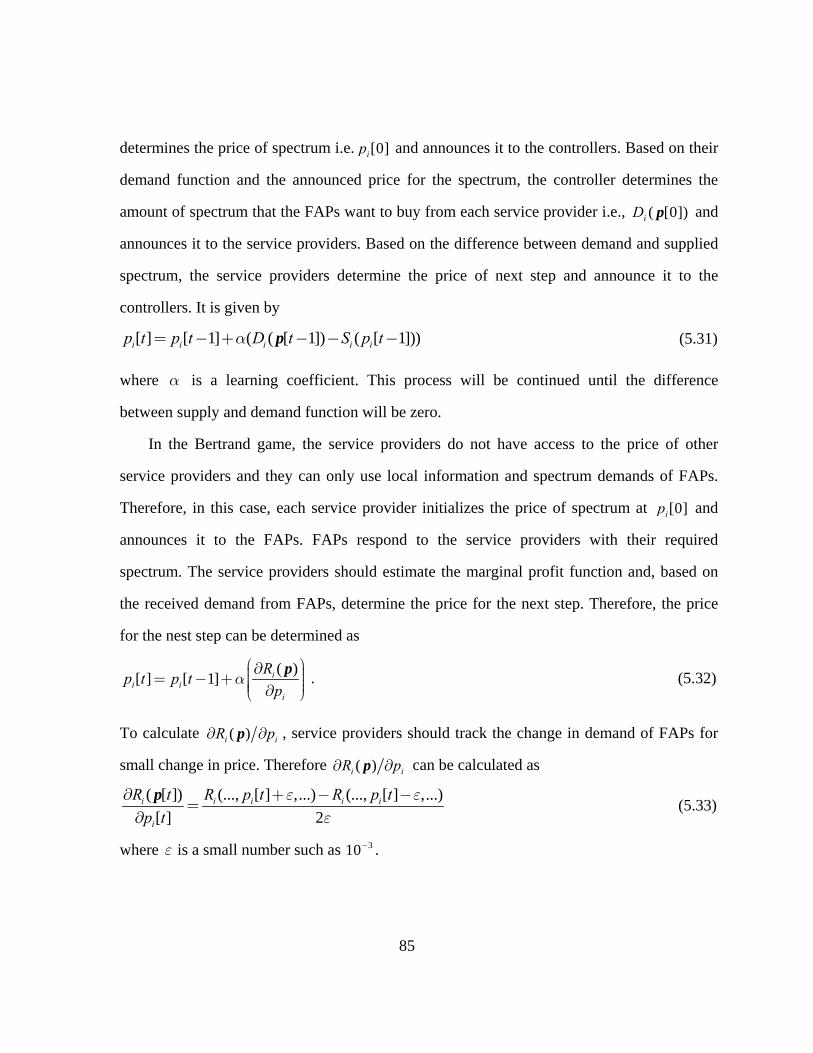
85
determines the price of spectrum i.e. [0]ip and announces it to the controllers. Based on their
demand function and the announced price for the spectrum, the controller determines the
amount of spectrum that the FAPs want to buy from each service provider i.e., ( [0])iD p and
announces it to the service providers. Based on the difference between demand and supplied
spectrum, the service providers determine the price of next step and announce it to the
controllers. It is given by
[ ] [ 1] ( ( [ 1]) ( [ 1]))i i i i ip t p t D t S p ta= - + - - -p (5.31)
where a is a learning coefficient. This process will be continued until the difference
between supply and demand function will be zero.
In the Bertrand game, the service providers do not have access to the price of other
service providers and they can only use local information and spectrum demands of FAPs.
Therefore, in this case, each service provider initializes the price of spectrum at [0]ip and
announces it to the FAPs. FAPs respond to the service providers with their required
spectrum. The service providers should estimate the marginal profit function and, based on
the received demand from FAPs, determine the price for the next step. Therefore, the price
for the nest step can be determined as
( )[ ] [ 1] i
i ii
Rp t p t
paæ ö¶ ÷ç ÷= - + ç ÷ç ÷ç ¶è ø
p . (5.32)
To calculate ( )i iR p¶ ¶p , service providers should track the change in demand of FAPs for
small change in price. Therefore ( )i iR p¶ ¶p can be calculated as
( [ ]) (..., [ ] ,...) (..., [ ] ,...)
[ ] 2i i i i i
i
R t R p t R p t
p t
e ee
¶ + - -=
¶p
(5.33)
where e is a small number such as 310- .
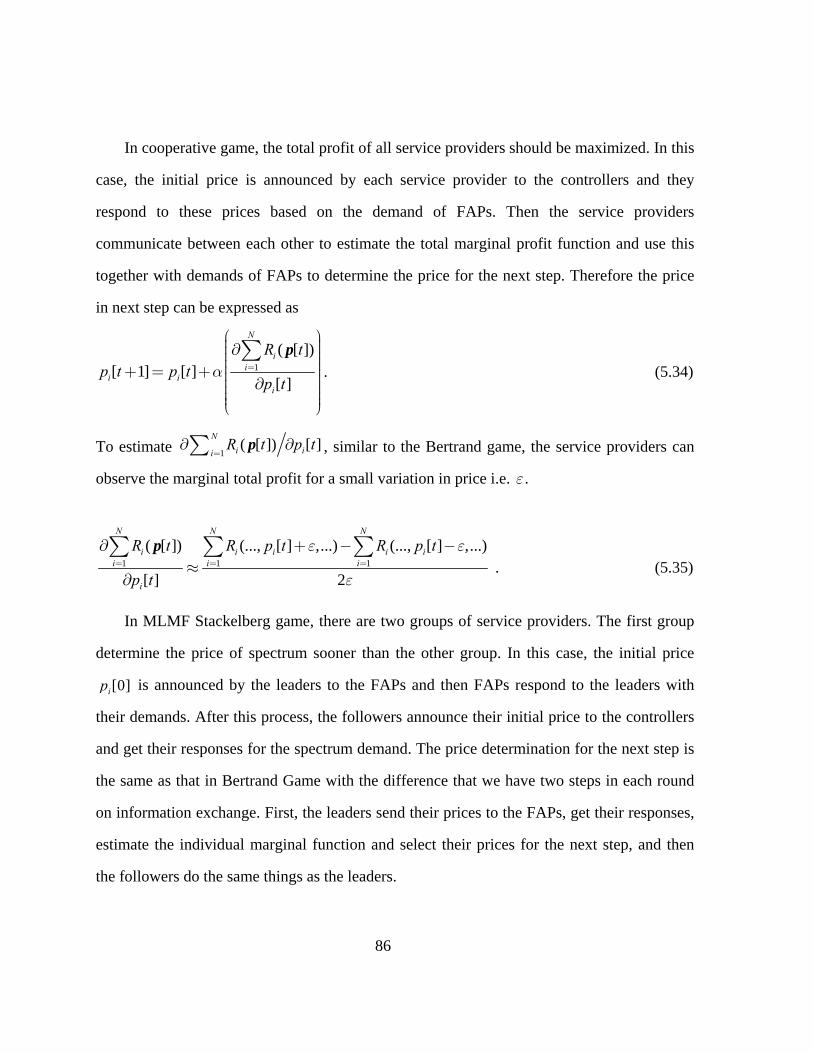
86
In cooperative game, the total profit of all service providers should be maximized. In this
case, the initial price is announced by each service provider to the controllers and they
respond to these prices based on the demand of FAPs. Then the service providers
communicate between each other to estimate the total marginal profit function and use this
together with demands of FAPs to determine the price for the next step. Therefore the price
in next step can be expressed as
1
( [ ])[ 1] [ ]
[ ]
N
ii
i ii
R tp t p t
p ta =
æ ö÷ç¶ ÷ç ÷ç ÷ç ÷+ = + ç ÷ç ÷¶ç ÷÷ç ÷ç ÷çè ø
å p. (5.34)
To estimate 1( [ ]) [ ]
N
i iiR t p t
=¶ ¶å p , similar to the Bertrand game, the service providers can
observe the marginal total profit for a small variation in price i.e. e .
1 1 1
( [ ]) (..., [ ] ,...) (..., [ ] ,...)
[ ] 2
N N N
i i i i ii i i
i
R t R p t R p t
p t
e e
e= = =
¶ + - -»
å å åp . (5.35)
In MLMF Stackelberg game, there are two groups of service providers. The first group
determine the price of spectrum sooner than the other group. In this case, the initial price
[0]ip is announced by the leaders to the FAPs and then FAPs respond to the leaders with
their demands. After this process, the followers announce their initial price to the controllers
and get their responses for the spectrum demand. The price determination for the next step is
the same as that in Bertrand Game with the difference that we have two steps in each round
on information exchange. First, the leaders send their prices to the FAPs, get their responses,
estimate the individual marginal function and select their prices for the next step, and then
the followers do the same things as the leaders.

87
5.5 Simulation and Numerical Results
In the simulations, we consider a macrocell system with two MBSs from two different
service providers. We assume that both of these MBSs are located at the center of a
hexagonal cell. The total frequency of each MBS is 30 MHZ. The distribution of FAPs and
MUEs are assumed to be CSPP with 10f , 5C , respectively. The FAPs are categorized
in the groups based on their distances from each other. The spectrum efficiency values of
both service providers 1M , 2M are assumed between 2 to 5 bit/sec/Hz. The spectrum
efficiency values of FUEs and MUEs iA , ik served by FAPs are assumed between 2 to 10
bit/sec/Hz. The required bandwidth of all FAP should be less than 80% of total bandwidth of
each service provider. 1C , 2C are assumed 0.7 and 0.8, respectively, which means that 0.7
and 0.8 of total selling bandwidth to FAPs are used for serving FUEs by FAPs. The
substitutability coefficient for FAPs is assumed 0.7v= .
In Fig.5.3 we show the supply and demand function with respect to the offered price
from the first service provider. We observe that the demand function is a decreasing function
of offered price and the spectrum supply is an increasing function of offered price. The
market equilibrium price is the point that supply and demand are equal together. It can be
also shown that market equilibrium price exists or does not exist for some FAPs or MBS
requirements.

88
Figure 5.3 Supply and demand functions in terms of price for service provider 1.
Fig.5.4 shows the best response of the service providers in the case of Bertrand game
and MLMF Stackelberg game. The intersection of best responses curves shows the Nash
equilibrium for Bertrand game. The location of Nash equilibrium is dependent on the
requirements of FAPs and MUEs as well as their demands. In the MLMF Stackelberg game,
it is assumed that the first service provider is the leader and sets the price of spectrum sooner
than the other second service provider. It can be observed that the Stackelberg equilibriums
for two service providers are different from Nash equilibrium in Bertrand game. In the
Stackelberg game, competition between service providers is less than Bertrand game and
leaders tend to set higher prices than the Bertrand game, since the followers have to set their
0 0.5 1 1.5 2 2.5 3 3.5 4 4.5 50
1
2
3
4
5
6
Price
Spe
ctru
m S
uppl
y/D
eman
d
Spectrum Demand
Spectrum Supply, M1=4.5, M
2=4.5
Spectrum Supply, M1=3.5, M
2=4.5
Spectrum Supply, M1=3, M
2=4.5
Market Equilibrium
No Market Equilibrium

89
prices after the leaders. Therefore, it can be seen that the prices in MLMF Stackelberg game
are more than those in Bertrand game.
Figure 5.4 Bertrand Game and MLMF Stackelberg game
Fig.5.5 shows the best response of the service providers in the case of cooperative game.
In a cooperative game, all the service providers cooperate with each other to maximize the
total revenue; therefore the price for the spectrum is more that all previous cases. In
application, to implement this type of pricing, service providers should communicate with
each other to reach Nash equilibrium.
0 0.5 1 1.5 2 2.5 3 3.5 4 4.5 50
0.5
1
1.5
2
2.5
3
3.5
4
4.5
5
Price for the first service provider ( p2 )
Pric
e fo
r th
e fir
st s
ervi
ce p
rovi
der
( p 1 )
Best Response for MBS 1
Best Response for MBS 2
Stackelberg Equilibrium for MBS 1
Nash Equilibrium
Stackelberg Equilibrium for MBS 2

90
Figure 5.5 Nash Equilibrium for Cooperative game
Fig.5.6 shows the total revenue of service providers from FAPs based on fixed pricing
[61], market equilibrium, Bertrand game, MLMF Stackelberg game and cooperative game
for OA. It can be observed that our proposed methods outperform fixed pricing in terms of
revenue for service provider. It can be seen that the total revenue of service providers in
cooperative game is more than that in other methods. The total revenue of service providers
in market equilibrium is less than other three methods in OA, since there is neither
competition nor cooperation between service providers. In the market equilibrium scheme,
the service providers are not aware of existence of each other and try to satisfy the demand
from FAPs. In this scheme, the service providers try to maximize the satisfaction of FAPs. In
the case of Bertrand game and Stackelberg game, the service providers are aware of the
0 1 2 3 4 5 60
1
2
3
4
5
6
Price for the second service provider (P2)
Pric
e fo
r th
e fir
st s
ervi
ce p
rovi
der
(P 1)
Best Response for MBS1
Best Response for MBS2
Nash Equilibrium for Cooperative game

91
competition between each other and try to set the unit price for spectrum to maximize their
revenue. But in Stackelberg game, the per unit price is more than the Bertrand game,
therefore the revenue of service providers are more than the Bertrand game.
Figure 5.6 Total profit of service providers from different methods
In Fig.5.7, we investigate effect of spectrum substitutability (v) on the spectrum price.
We set all specifications of two service providers the same as each other. For 0v = , the
FAPs cannot change its operating spectrum but when 1v = , the FAPs can switch between
service providers freely. It can be observed that with increasingv, the spectrum price for the
first service provider decreases in all four proposed methods. It is also observed that the
spectrum price has the highest value for all values of v under cooperative game and has the
lowest price for the market equilibrium. For 0v = , the Bertrand game and MLMF
01
23
45
67
0
2
4
6
8
15
20
25
30
35
40
Price for the second service providerPrice for the first service provider
Tot
al r
even
ue f
or t
he s
ervi
ce p
rovi
ders
Cooperative game
Stackelberg game
Bertrand gameMarket Equilibrium
Fixed Pricing Open Access

92
Stackelberg game have the same price as the cooperative game, since the FAPs cannot switch
between service providers, therefore there is no competition between service providers. For
1v = , the level of competition between service providers are high and service providers
should decrease the spectrum prices to attract more FAPs.
Figure 5.7 Spectrum price in terms of spectrum substitutability (v)
0 0.1 0.2 0.3 0.4 0.5 0.6 0.7 0.8 0.9 12.5
3
3.5
4
4.5
5
5.5
substitutability coefficient (v)
Spe
ctru
m P
rice
for
the
first
ser
vice
pro
vide
r
Cooperative game
Stackelberg game
Bertrand game
Market Equilibrium

93
Chapter 6
Conclusions and Future Work
In this chapter, we first provide the conclusion of research work done so far, then
provide some future research directions.
6.1 Conclusions
Cognitive radio and femtocell networks are two emerging concepts for innovative
spectrum utilization. A common feature of cognitive radio and femtocells is their two-tier
nature involving primary and secondary users. Two main challenges in two-tier networks is
the design of efficient resource allocation and pricing methods which we have addressed in
this thesis.
In Chapter 2, we have considered the spectrum trading problem for shared used model in
cognitive radio networks. We have designed a multi-unit sequential sealed-bid first-price
auction taking into accounts risks due to imperfect sensing. We have derived an expression
for the total revenue of WSP and maximized it by optimizing the sensing time. Our
numerical results have demonstrated that the proposed bidding strategy outperforms the
conventional one (i.e., designed ignoring any risk) in a risky environment. For some typical
values of probability of miss and number of SUs, it was found out that the payoff of bidders
by our proposed method is at least two times and in best case, five times more than that can
be obtained from the conventional one. Our results have further revealed that maximization
of throughput is not necessary to get the maximum revenue.
In Chapter 3, we have investigated the sensing-throughput tradeoff in a cognitive radio
network with cooperative sensing over time varying fading channels. First, we have derived
an expression for the total average throughput of the SUs each of which is equipped with
energy detectors. Then we have formulated a throughput optimization problem and solved

94
this based on a two-step algorithm. The first step involves the calculation of the optimal
sensing time based on a non-linear programming problem. The second step involves finding
the optimum number of SUs for each channel to maximize the total throughput. The
numerical results demonstrate that our proposed method based on joint optimization of the
sensing time and the number of sensing SUs for each channel over conventional cases than in
which either the sensing time is fixed or the number of sensing SUs is fixed.
In Chapter 4, we have considered the spectrum trading problem for non-identical
channels under the assumption of exclusive usage model in a cognitive radio network. We
have proposed a realistic valuation function for the SUs which depends on delay-sensitive/-
insensitive traffic as well as the capacity of each available channel. Instead of the commonly
assumed single-minded bidders, we have assumed r -minded SU bidders and designed an
efficient VCG-based auction mechanism. In our scheme, each bidder can bid for r bundles
of channels in each round of auction, but each bidder is allowed to win at most one of these
bundles. We have investigated two cases: In the first case, the SUs are r -minded but they can
submit bid only for single channels. In the second case, the SUs are r -minded and they can
submit bid for bundles of channels. We have shown that the first case is solvable in
polynomial time but in the other one, the problem of determining auction outcomes is NP-
hard. We have proposed two sub-optimal methods for solving this problem, namely greedy
algorithm and randomized rounding linear programming (LP) relaxation. In the numerical
results, we have demonstrated that the revenue of auctioneer increases with the increasing
number of bidders and submitted bids. The average profit of bidders also increases with the
increasing number of submitted bids when the number of bidders is around the number of
channels. When the number of bidders is two times or more than number of channels, the
average profit of bidders degrades with the increase in the number of submitted bids. Due to
the sub-optimal nature of solutions in the second case, VCG mechanism is not truthful

95
anymore and the SUs can lie to maximize their utilities. To address this, we have proposed an
auction mechanism with limited truthfulness property, based on an iterative greedy
algorithm.
In Chapter 5, we have introduced pricing schemes for OA femtocell networks.
Specifically, we have proposed four dynamic pricing schemes based on market equilibrium,
Bertrand game, multiple-leader-multiple-follower Stackelberg game and cooperative game.
In the first scheme, service providers are not aware of each other and try to satisfy the
demand of FAPs. In this scheme, satisfaction and incentive of FAPs to participate in OA
model are maximized. In Bertrand game, service providers compete with each other to
determine the price of spectrum. In this scheme, the revenue of service providers are more
and the satisfaction of FAPs are less than previous scheme. In multiple-leader-multiple-
follower Stackelberg game, there are some service providers who enter femtocell market
sooner that the others and they can set the price of spectrum before the others which they
called leaders and other service providers called followers should set the spectrum price after
them. In cooperative game, the service providers try to maximize the total revenue of all of
them. We have compared the performance of our schemes and shown that the cooperative
game outperforms the other methods in terms of revenue for service providers. On the other
hand, we have demonstrated that the pricing scheme based on market equilibrium outperform
other methods in terms of FAP satisfaction.
6.2 Future Works
Based on the discussion in Chapter 2, we have assumed that all available channels have
the same risks, therefore same risks are taken account for all of them in optimal bidding
calculation. In cases where the detection and false alarm probabilities are different for

96
underlying channels, these derivations need to be revisited. On the other hand, we have not
considered the chance of PUs who enter the channels during the SUs transmission. This can
be further considered as another practical constraint.
In auction mechanism, the SUs are selfish and they aim to maximize their profit. They
may cheat or collude in the spectrum auction if profitable, which ruins the auction and
therefore the auction mechanisms should be resistant to bidders collusion. In Chapter 3, we
have proposed truthful auction mechanism for non-identical channel allocation. In truthful
auction mechanism, the bidders prevent from lying about their valuation, but they can
collude together to maximize their profit. Therefore it would a good idea to extend the
auction mechanism in chapter 3 to a collusion resistant and truthful auction for non-identical
channel allocation.
To ensure minimal impact on the performance of the existing MBSs, femtocell network
needs to be designed with smart resource allocation and interference management strategies.
As we mentioned in chapter 1, towards this overall purpose, game theory can be used as a
natural design methodology for resource allocation in such an interference-limited
environment where there are different rational entities with different types of demands. Two
different game-theoretic approaches can be considered for different scenarios based on the
availability of information exchange between two tiers in femtocell networks. Non-
cooperative game-theoretic approach can be used for a deployment scenario where there is
no information exchange between femtocell and macrocell tiers, but information exchange is
allowed between nearby FAPs. Also a bargaining game formulation can be used in situations
where we can assume some information exchange between femtocell and macrocell tiers
along with the femtocell-to-femtocell information exchange.
97
Appendix A
Proof of Theorem 3.1
In this Appendix, we will show that three conditions in (3.7)-(3.9) are satisfied in our
case. In the following, without loss of generality, we ignore index i for simplicity.
1) Condition in (2.7): For this condition, we need to show that the mean value of 2| ( ) |y n
takes finite values. Replacing (3.1) within, we have
2 2 2E | ( ) | E | ( ) ( ) ( ) | ( 1) uy n h n s n u n (A.1)
2h , 2
s and 2u have limited values, therefore (2.7) is satisfied.
2) Condition in (3.8): For (3.8), we need to show that the variance of 2| ( ) |y n takes finite
values. Replacing (3.1) within, we have
2
2 2 4 4 4 2 2 2 2
| |Var | ( ) | = E | ( ) | E | ( ) | E | ( ) | ( )h s uy
y n h n s n u n . (A.2)
In our case, ( )is n is a rectangular M-QAM modulation signal with zero mean and
variance 2s . Therefore, we have
4 43 3 7E | ( ) |
10 1i s
Ms n
M
.
(A.3)
Inserting 4 4E | ( ) | 2i hh n , 4 4E | ( ) | 2i uu n and (A.3), we have
2
2 4 2
| |
3 3 71 2 1
5 1uy
M
M
. (A.4)
Since the SNR and noise power have limited values, it can be concluded that 2
2
| |y .
Therefore the second condition given by (2.8) is satisfied. It should be noted that this
condition can be satisfied with any type of limited energy signal and limited noise power.
3) Condition in (3.9): We need to show that

98
2
2 2 2
| |2
lim Var[ ( )] 2 Cov | (1) | ,| ( ) |N
yNi
N y y y i V
(A.5)
takes finite values. Since we have already shown that 2
2
| |y is limited, it is sufficient to prove
that the second summation term is finite. We first focus on a single term inside the
summation, i.e.,
2 2 2 2
2 2
Cov | ( ) | ,| ( ) | E | ( ) ( ) ( ) | | ( ) ( ) ( ) |
E | ( ) ( ) ( ) | E | ( ) ( ) ( ) |
y i y j h i s i u i h j s j u j
h i s i u i h j s j u j
. (A.6)
Since ( )s n , ( )u n , and ( )h n are assumed independent of each other and have zero mean,
it is straightforward to show that (A.6) can be simplified as
2 2 2 2 2 2 2 2Cov | ( ) | ,| ( ) | E | ( ) | | ( ) | E | ( ) | | ( ) | E | ( ) | E | ( ) |y i y j s i s j h i h j h i h j . (A.7)
Replacing ( ) ( ) ( )R Ih i h i jh i in (A.7) and noting that ( )Rh i , ( )Ih i are independent
from each other, (A.7) can be rewritten as
2 2 4 4 2( )Cov | ( ) | , | ( ) | s h j iy i y j (A.8)
where ( ) E ( ), ( ) E ( ), ( )R R I Ij i h i h j h i h j . Based on Parseval equality, we have
2 2
1( ) | S( ) |
nn f df
, where S( )f is Doppler PSD function. The integration of
Doppler PSD under Jakes model within the range of ,d df f yields infinity. However, in
simulations, a truncated Jakes model is commonly used to avoid the singularities at the edges
[101], [102]. Through truncation of the channel impulse response, we have
2
1 1, 0
1
d
d
f
df d
dff f f
. (A.9)
Therefore, we can conclude that we have 4 4 2
1lim
N
s h iiN
for the truncated version
of Jakes model.

99
Appendix B
Proof of Theorem 3.2
In this Appendix, we show that three conditions in (3.25)-(3.27) are satisfied for majority
logic rule, therefore ( )iiR is unimodal in the range of 0 i T . In the following, without
loss of generality, we ignore index i in the following equations for simplicity.
1) Condition in (3.25): First we need to obtain ( )R which is given as:
0 0
( )( ) (H ) 1 ( ) 1 f
fR C P T
(B.1)
where ( )f can be calculated as
2 12( ) ( )2 (1 ( )) ( )
2
kk kf ff f
k Pk P P
k
(B.2)
where
2
( ) exp28
fP
(B.3)
sf and,
1 2 2
1
3 3 7( ) 1 2 2 1
5 1
N
d ii
MQ P
M
. (B.4)
At 0 , ( )fP , and hence ( )f for majority logic rule. Therefore
( ) 0R and the first condition is satisfied.
2) Condition in (3.26): At T , we obtain 0 0( ) (H ) 1 ( )fR C P . For
0 ( ) 1fP ( ) 1f , therefore ( ) 0R and the second condition is satisfied.

100
3) Condition in (3.27): Set ( ) 0R and after simplifications we have
/2 1 2/2/2 1
0
82ln (1 ( )) ( , )
2
kk ii k
f fi
kP P
ikk T
k
(B.5)
Eq. (3.27) is satisfied if the right hand side (RHS) and the left hand side (LFS) of (B.4)
intersect each other only once in the range of 0 T . It can be shown that RHS is
monotonically decreasing for | 0,0L T and monotonically
increasing for | 0,0H T . It can be further shown that LHS is
monotonically decreasing for 0 T and decreasing rate of LHS is faster than the RHS.
If RHS and LFS intersect in the L region, it is impossible for them to intersect more
than once in L region because LHS is decreasing at a faster rate than RHS. Since RHS is
increasing in H region, RHS and LHS cannot intersect with each other if they have
intersected in L region.
If RHS and LHS do not intersect in the L region, they must intersect with each other in
H region. Since RHS is monotonically increasing and LHS is monotonically decreasing in
this region, therefore they can intersect only once with each other. Hence, we show that if
LHS and RHS intersect with each other in either L or H , they can intersect only once
with each other and therefore (3.27) is satisfied.

101
Appendix C
Proof of Theorem 4.1
This appendix provides the proof of Theorem 4.1. Assume a hyper-graph ( , ),G = B W E
that consists of two disjoint sets of vertices denoted by B and W . Here, B is the set of
bidders that each bidder is represented by a vertex. W is a set of channels each of which is
represented by a vertex. When a bidder wants to bid for a bundle of channels, we take into
account an edge consisting the vertex of the bidder in set B and vertices of the channels in
set W . For example, assume that there are 4 bidders and 3 channels for sale and each bidder
can submit 2 bids, the bidding of bidders can be represented as illustrated in Fig. C.1.
Determining the optimal allocation among bidders involves finding a collection of disjoint
sets that has the maximum total weight. Now assume a set Z of winners with disjoint
elements, the social welfare obtained by Z is exactly the size of this set. It follows that an
independent set with the weight of at least q exists if and only if the social welfare of the
optimal allocation is at least q . This concludes NP-hardness proof.
Fig. C.1 Modeling r-minded bidders in case 2

102
Appendix D
Proof of Theorem 4.2
This appendix provides the proof of Theorem 4.2. Assume that we model the auction
mechanism with a hyper-graph consisting of M N vertices which they can be divided in
two separate sets. The number of hyper-edges is rN and the maximum cardinality of each
hyper-edge is m . Let iW and | K | 1i is denote weight and the number of items in each
hyper-edge. The norm of each hyper-edge is given by i i in W s . Assume that the
optimum solution for this problem is iopt i optWSWF and the solution of greedy algorithm
is gr i gr iSWF W . We need to show that the following inequality holds:
min ,opt grSWF SWF m M . (D.1)
First, we will prove opt grSWF SWF M , then show that opt grSWF SWF m holds.
Without loss of generality, we assume that there is no common hyper-edge in optimum and
greedy solutions. If there are any hyper-edges in common in two solutions, the common
hyper-edge and vertices can be removed and the new problem becomes similar to the original
one. By doing some algebraic computation for greedy solution, we have
2 2gr i i i
i gr i gr
SWF W n s
. (D.2)
By applying the Cauchy-Schwarz inequality for optimum solution, we obtain
2opt i i i i i
i opt i opt i opt i opt
SWF W n s n s
. (D.3)
Noting that ii optS is the total number of items allocated optimally to the bidders and
therefore it is bounded by M , we can conclude
2opt i i
i opt i opt
SWF n s
. (D.4)

103
Now, we need to show that 2 2i i ii opt i gr
n n s
. We have assumed that there is no
joint bid between optimum and greedy algorithm. This means that if a hyper-edge or a bid i
from optimal solution is considered within the execution of greedy algorithm, it cannot be
entered in the partial allocation already built. This implies that there is an item that has been
already allocated in the partial greedy solution. Therefore there is a bid j in greedy
algorithm with j in n and that item also belongs to bid j . In optimal solution, there are at
most is different bids associated with bid j of greedy algorithm, since the sets of items
requested by two different bids of optimal solution do not have any intersection. If we
assume that jop is the set of hyper-edges or bids of optimal solution that are associated with
bid j , we can write
2 2
j
i j ji op
n n s
. (D.5)
Therefore we can conclude 2 2i i ii op i gr
n n s
from (D.5) and the first part of theorem
is proven.
For the second part, based on the above explanation, we conclude that j
i j ji opn n s
. From
the definition of norm, we have i i in W s , therefore j
i j ji opn s W
. The number of
items in a bid is m at most, thus m M . By the same conclusion as in (D.5), we have
ii i gri opWn m
.
On the other hand, we have opt i ii opt i optSWF W m n
and iopt i op
nSWF m
therefore we conclude that min ,opt grSWF SWF m M . If 1 2l it can be shown that
the approximation algorithm will be max 1/ ,1 /m M .

104
Appendix E
Solving Linear Equations in (5.9)
In this appendix, we want to solve set of linear equations in (5.9). (5.9) can be rewritten in
matrix form as
1 1 2 1 1 1
1 2 2 2 2 2
1 2
N
N
N N N N N
X V Y Y p l q
Y X V Y p l q
Y Y X V p l q
é ù é ù é ù- -ê ú ê ú ê úê ú ê ú ê ú- -ê ú ê ú ê ú=ê ú ê ú ê úê ú ê ú ê úê ú ê ú ê ú- -ë û ë û ë û
A p Q
. (E.1)
Therefore to solve (E.1), first we should calculate 1-A . There is a lemma in [103] for
calculation of 1-A .
Lemma: If we can write matrix A = G + H where G is non-singular and H has rank of
one.
( ) 11 1 1 11
1 g-- - - -= -
+A = G + H G G HG (E.2)
where 1( )g tr -= HG .
We can write G and H as
1 1 1 1 2
2 2 2 1 2
1 2
0 0
0 0,
0 0
N
N
N N N N
X V Y Y Y Y
X V Y Y Y Y
X V Y Y Y Y
é ù é ù- -ê ú ê úê ú ê ú- -ê ú ê ú= ê ú ê úê ú ê úê ú ê ú- -ë û ë û
G H = . (E.3)
Therefore 1-A can be calculated as N N´ matrix which the elements on the diagonal of
matrix are
( )1
2
1
1 1
1
iii N
ii i i i i i
i i i i
Ya
YX V Y X V YX V Y
-
=
æ ö÷ç ÷ç= - ÷ç ÷ç- - ÷ç - -è ø+- -å
. (E.4)

105
The other elements of 1-A are
( )( )1
1
1,
1
jij N
k i i i j j j
k k k k
Ya i j
Y X V Y X V YX V Y
-
=
æ ö÷ç ÷ç=- ¹÷ç ÷ç ÷- - - - ÷çè ø+- -å
(E.5)

106
Bibliography
[1] “National Broad Band Plan of United State. [Online] Available:” .
[2] J. Mitola, Cognitive radio: An Integrated Agent Architecture for Software Defined
Radio. Royal Institute of Technology,Sweden, 2000.
[3] “IEEE 802.22 Working Group on Wireless Regional Area Networks,” .
[4] V. Chandrasekhar, J. Andrews, and A. Gatherer, “Femtocell networks: a survey,” IEEE
Commun. Mag., vol. 46, no. 9, pp. 59 –67, Sep. 2008.
[5] “Small Cell Market Status - Informa.” Small Cell Forum, Feb-2013.
[6] “http://www.femtoforum.org.” .
[7] D. Niyato, E. Hossain, and Z. Han, “Dynamic spectrum access in IEEE 802.22- based
cognitive wireless networks: a game theoretic model for competitive spectrum bidding
and pricing,” IEEE Wireless Commun., vol. 16, no. 2, pp. 16 –23, Apr. 2009.
[8] E. Hossain, D. Niyato, and Z. Han, Dynamic Spectrum Access and Management in
Cognitive Radio Networks, Cambridge University Press, 1st ed., 2009.
[9] S. Maharjan, Y. Zhang, and S. Gjessing, “Economic Approaches for Cognitive Radio
Networks: A Survey,” Wireless Pers. Commun., vol. 57, no. 1, pp. 33–51, Mar. 2011.
[10] C. A. Gizelis and D. D. Vergados, “A Survey of Pricing Schemes in Wireless
Networks,” IEEE Commun. Surveys Tuts., vol. 13, no. 1, pp. 126 –145, quarter 2011.
[11] R. B. Myerson, Game Theory: Analysis of Conflict, Reprint. Harvard University Press,
1997.
[12] A. A. Cournot, Researches into the mathematical principles of the theory of wealth,
1838. With an essay, Cournot and mathematical economics and a Bibliography of
mathematical economics. New York, A. M. Kelley, 1971.
[13] C. U. Saraydar, N. B. Mandayam, and D. J. Goodman, “Efficient power control via
pricing in wireless data networks,” IEEE Trans. on Commun., vol. 50, no. 2, pp. 291 –
303, Feb. 2002.

107
[14] Z. Han, Z. Ji, and K. J. R. Liu, “Power minimization for multi-cell OFDM networks
using distributed non-cooperative game approach,” in Proc. IEEE Global Telecommun.
Conf., (GLOBECOM), Dallas, USA, 2004.
[15] Z. Han, Z. Ji, and K. J. R. Liu, “Fair Multiuser Channel Allocation for OFDMA
Networks Using Nash Bargaining Solutions and Coalitions,” IEEE Trans. on Commun.,
vol. 53, no. 8, pp. 1366 – 1376, Aug. 2005.
[16] H. Park and M. van der Schaar, “Bargaining Strategies for Networked Multimedia
Resource Management,” IEEE Trans. on Signal Process., vol. 55, no. 7, pp. 3496 –
3511, Jul. 2007.
[17] D. Grandblaise, C. Kloeck, T. Renk, P. Bag, P. Levine, K. Moessner, J. Yang, M. Pan,
and K. Zhang, “Microeconomics Inspired Mechanisms to Manage Dynamic Spectrum
Allocation,” in Proc 2nd IEEE International Symposium on New Frontiers in Dynamic
Spectrum Access Networks., DySPAN, Dublin, Ireland, 2007.
[18] A. Mas-Colell, M. D. Whinston, and J. R. Green, Microeconomic Theory. Oxford
University Press, 1995.
[19] “N. Bernoulli; acknowledging receipt of ‘Specimen theoriae novae metiendi sortem
pecuniariam’, letter of 5 April 1732.”.
[20] E. L. Grant, W. G. Ireson, and R. S. Leavenworth, Principles of Engineering Economy,
8th ed. Wiley, 1990.
[21] T. Yucek and H. Arslan, “A survey of spectrum sensing algorithms for cognitive radio
applications,” IEEE Commun. Surveys Tut., vol. 11, no. 1, pp. 116 –130, quarter 2009.
[22] D. Niyato and E. Hossain, “Spectrum trading in cognitive radio networks: A market-
equilibrium-based approach,” IEEE Wireless Commun., vol. 15, no. 6, pp. 71 –80, Dec.
2008.
[23] D. Niyato and E. Hossain, “Market-Equilibrium, Competitive, and Cooperative Pricing
for Spectrum Sharing in Cognitive Radio Networks: Analysis and Comparison,” IEEE
Trans. on Wireless Commun., vol. 7, no. 11, pp. 4273 –4283, Nov. 2008.

108
[24] H.-B. Chang and K.-C. Chen, “Auction-Based Spectrum Management of Cognitive
Radio Networks,” IEEE Trans. on Veh. Tech., vol. 59, no. 4, pp. 1923 –1935, May
2010.
[25] S. Sengupta and M. Chatterjee, “Designing Auction Mechanisms for Dynamic
Spectrum Access,” Mobile Netw. Appl., vol. 13, no. 5, pp. 498–515, Oct. 2008.
[26] Z. Ji and K. J. R. Liu, “Multi-Stage Pricing Game for Collusion-Resistant Dynamic
Spectrum Allocation,” IEEE J. on Sel. Areas in Commun., vol. 26, no. 1, pp. 182 –191,
Jan. 2008.
[27] L. Lei, Z. Zhong, C. Lin, and X. Shen, “Operator controlled device-to-device
communications in LTE-advanced networks,” IEEE Wireless Commun., vol. 19, no. 3,
pp. 96 –104, Jun. 2012.
[28] D. Niyato and E. Hossain, “Hierarchical Spectrum Sharing in Cognitive Radio: A
Microeconomic Approach,” in IEEE Wireless Commun. and Netw. Conf (WCNC),
Honk Kong, 2007.
[29] V. Krishna, Auction Theory. Academic Press, 2002.
[30] N. Shetty, S. Parekh, and J. Walrand, “Economics of Femtocells,” in IEEE Global
Telecommun. Conf. (GLOBECOM), Honolulu, USA, 2009.
[31] V. Rodriguez and R. Mathar, “Simple decentralised market-oriented management of
OFDMA femto-cells,” in Proc of the 6th International Wireless Commun. and Mobile
Computing Conf. (IWCMC), New York, NY, USA, 2010.
[32] S. Hua, X. Zhuo, and S. S. Panwar, “A Truthful Auction based Incentive Framework
for Femtocell Access,” arXiv:1210.5012, Oct. 2012.
[33] Y. Chen, J. Zhang, Q. Zhang, and J. Jia, “A reverse auction framework for access
permission transaction to promote hybrid access in femtocell network,” in Proc IEEE
International Conf. on Computer and Commun. (INFOCOM), Orlando, USA, 2012.
[34] H. Nabih Agiza, G. Italo Bischi, and M. Kopel, “Multistability in a dynamic Cournot
game with three oligopolists,” Mathematics and Computers in Simulation, vol. 51, no.
1–2, pp. 63–90, Dec. 1999.

109
[35] Y.-P. J. Hsu and X. Wang, “On Welfare under Cournot and Bertrand Competition in
Differentiated Oligopolies,” Review of Industrial Organization, vol. 27, no. 2, pp. 185–
191, 2005.
[36] D. Niyato and E. Hossain, “Competitive Pricing for Spectrum Sharing in Cognitive
Radio Networks: Dynamic Game, Inefficiency of Nash Equilibrium, and Collusion,”
IEEE J. on Sel. Areas in Commun., vol. 26, no. 1, pp. 192 –202, Jan. 2008.
[37] L. S. Shapley, “Stochastic Games,” PNAS, vol. 39, no. 10, pp. 1095–1100, Oct. 1953.
[38] K. R. Apt and T. Radzik, “Stable partitions in coalitional games,” arXiv:cs/0605132,
May 2006.
[39] F. Fu and M. van der Schaar, “Learning to Compete for Resources in Wireless
Stochastic Games,” IEEE Trans. on Veh. Tech., vol. 58, no. 4, pp. 1904 –1919, May
2009.
[40] Z. Han, Z. Ji, and K. J. R. Liu, “Non-cooperative resource competition game by virtual
referee in multi-cell OFDMA networks,” IEEE J. on Sel. Areas in Commun., vol. 25,
no. 6, pp. 1079 –1090, Aug. 2007.
[41] G. Hosseinabadi, H. Manshaei, and J. P. Hubaux, “Spectrum sharing games of
infrastructure-based cognitive radio networks.” Technical Report LCA-REPORT, 2008.
[42] V. Chandrasekhar, J. G. Andrews, T. Muharemovic, Z. Shen, and A. Gatherer, “Power
control in two-tier femtocell networks,” IEEE Trans. on Wireless Commun., vol. 8, no.
8, pp. 4316 –4328, Aug. 2009.
[43] S. Barbarossa, S. Sardellitti, A. Carfagna, and P. Vecchiarelli, “Decentralized
interference management in femtocells: A game-theoretic approach,” in Proc. of the
Fifth International Conf. on Cognitive Radio Oriented Wireless Networks Commun.
(CROWNCOM), Cannes, France, 2010.
[44] Y.-C. Liang, Y. Zeng, E. C. Y. Peh, and A. T. Hoang, “Sensing-Throughput Tradeoff
for Cognitive Radio Networks,” IEEE Trans. on Wireless Commun., vol. 7, no. 4, pp.
1326 –1337, Apr. 2008.

110
[45] M. Cardenas-Juarez and M. Ghogho, “Spectrum Sensing and Throughput Trade-off in
Cognitive Radio under Outage Constraints over Nakagami Fading,” IEEE Commun.
Lett., vol. 15, no. 10, pp. 1110–1113, October.
[46] Y. Zou, Y.-D. Yao, and B. Zheng, “Outage Probability Analysis of Cognitive
Transmissions: Impact of Spectrum Sensing Overhead,” IEEE Trans. on Wireless
Commun., vol. 9, no. 8, pp. 2676–2688, August.
[47] G. Noh, J. Lee, H. Wang, S. Kim, S. Choi, and D. Hong, “Throughput Analysis and
Optimization of Sensing-Based Cognitive Radio Systems With Markovian Traffic,”
IEEE Trans. on Veh. Tech., vol. 59, no. 8, pp. 4163–4169, Oct.
[48] E. C. Y. Peh, Y.-C. Liang, Y. L. Guan, and Y. Zeng, “Optimization of Cooperative
Sensing in Cognitive Radio Networks: A Sensing-Throughput Tradeoff View,” IEEE
Trans. on Veh. Tech., vol. 58, no. 9, pp. 5294–5299, Nov.
[49] E. Peh and Y.-C. Liang, “Optimization for Cooperative Sensing in Cognitive Radio
Networks,” in IEEE Wireless Commun. and Netw. Conf. (WCNC), Honk Kong, 2007.
[50] W. Zhang, R. Mallik, and K. Letaief, “Optimization of cooperative spectrum sensing
with energy detection in cognitive radio networks,” IEEE Trans. on Wireless Commun.,
vol. 8, no. 12, pp. 5761 –5766, Dec. 2009.
[51] Z. Khan, J. Lehtomaki, M. Latva-aho, and L. A. DaSilva, “On selfish and altruistic
coalition formation in cognitive radio networks,” in Proc. of the Fifth International
Conf. on Cognitive Radio Oriented Wireless Netw. Commun. (CROWNCOM), Cannes,
France, 2010.
[52] B. Wang, K. J. R. Liu, and T. C. Clancy, “Evolutionary cooperative spectrum sensing
game: how to collaborate?,” IEEE Trans. on Commun., vol. 58, no. 3, pp. 890–900,
March.
[53] H. Kim and K. G. Shin, “Optimal admission and eviction control of secondary users at
cognitive radio HotSpots,” in Proc. of the 6th Annual IEEE commun. society conf. on
Sensor, Mesh and Ad Hoc Communications and Networks (SECON), Piscataway, NJ,
USA, 2009.

111
[54] D. T. Ngo, C. Tellambura, and H. H. Nguyen, “Resource Allocation for OFDMA-
Based Cognitive Radio Multicast Networks With Primary User Activity Consideration,”
IEEE Trans. on Veh. Tech., vol. 59, no. 4, pp. 1668 –1679, May 2010.
[55] A. Goldsmith, Wireless Communications. Cambridge University Press, 2005.
[56] G. S. Kasbekar and S. Sarkar, “Spectrum Auction Framework for Access Allocation in
Cognitive Radio Networks,” IEEE/ACM Trans. on Netw., vol. 18, no. 6, pp. 1841 –
1854, Dec. 2010.
[57] Z. Han, R. Zheng, and H. V. Poor, “Repeated Auctions with Bayesian Nonparametric
Learning for Spectrum Access in Cognitive Radio Networks,” IEEE Trans. on Wireless
Communic., vol. 10, no. 3, pp. 890 –900, Mar. 2011.
[58] N. Nisan, T. Roughgarden, E. Tardos, and V. V. Vazirani, Eds., Algorithmic Game
Theory, Cambridge University Press, 1st ed., 2007.
[59] N. Nisan and A. Ronen, “Computationally Feasible VCG Mechanisms,” in In ACM
Conf. on Electronic Commerce, Minneapolis, USA, 2000.
[60] S. Yun, Y. Yi, D.-H. Cho, and J. Mo, “Open or close: On the sharing of femtocells,” in
Proc. IEEE INFOCOM, Shanghai, China, 2011.
[61] S.-Y. Yun, Y. Yi, D.-H. Cho, and J. Mo, “The Economic Effects of Sharing
Femtocells,” IEEE J. on Sel. Areas in Commun., vol. 30, no. 3, pp. 595 –606, Apr.
2012.
[62] Q. Zhao, L. Tong, A. Swami, and Y. Chen, “Decentralized cognitive MAC for
opportunistic spectrum access in ad hoc networks: A POMDP framework,” IEEE J. on
Sel. Areas in Commun., vol. 25, no. 3, pp. 589 –600, Apr. 2007.
[63] J. Proakis and M. Salehi, Digital Communications, 5th Edition, 5th ed. McGraw-Hill
Science/Engineering/Math, 2007.
[64] R. Durrett, Probability: Theory and Examples, 4th ed. Cambridge University Press,
2010.
[65] J. E. Dennis and R. B. Schnabel, Numerical Methods for Unconstrained Optimization
and Nonlinear Equations. Society for Industrial and Applied Mathematics, 1987.

112
[66] C.-D. Iskander and P. T. Mathiopoulos, “Analytical level crossing rates and average
fade durations for diversity techniques in Nakagami fading channels,” IEEE Trans. on
Commun., vol. 50, no. 8, pp. 1301–1309, Aug.
[67] M. A. Trick, “A Dynamic Programming Approach for Consistency and Propagation for
Knapsack Constraints,” in Annals of Operations Research, 2001, pp. 113–124.
[68] J. Zhu and S. Li, “Channel allocation mechanisms for cognitive radio networks via
repeated multi-bid auction,” in 2006 IET International Conf. on Wireless, Mobile and
Multimedia Networks (ICWMMN), Hangzhou, China, 2006.
[69] R. Lavi and C. Swamy, “Truthful and Near-Optimal Mechanism Design via Linear
Programming,” in Proceedings of the 46th Annual IEEE Symposium on Foundations of
Computer Science (FCOS), Washington, DC, USA, 2005.
[70] D. Lehmann, L. I. O’callaghan, and Y. Shoham, “Truth Revelation in Rapid,
Approximately Efficient Combinatorial Auctions,” in In ACM Conf. on Electronic
Commerce (EC), Denver, USA, 1999.
[71] K. Mulmuley, U. V. Vazirani, and V. V. Vazirani, “Matching is as easy as matrix
inversion,” in Proc. of the nineteenth annual ACM symposium on Theory of computing
(STOC), New York, NY, USA, 1987.
[72] R. E. Tarjan, Data Structures and Network Algorithms. SIAM, 1983.
[73] A. Frank, “On Kuhn’s Hungarian Method—A tribute from Hungary,” Naval Research
Logistics (NRL), vol. 52, no. 1, pp. 2–5, 2005.
[74] M. N. Tehrani and M. Uysal, “Spectrum trading for non-identical channel allocation in
cognitive radio networks,” in 2011 IEEE 22nd International Symp. on Pers. Indoor and
Mobile Radio Commun. (PIMRC), Toronto, Canada, 2011.
[75] A. Srinivasan, “Approximation Algorithms Via Randomized Rounding: A Survey,” in
Series in Advanced Topics in Mathematics, Polish Scientific Publishers PWN, 1999, pp.
9–71.
[76] D. Parkes, “iBundle: An Efficient Ascending Price Bundle Auction,” in In ACM Conf.
on Electronic Commerce (EC), Denver, USA, 1999.

113
[77] L. Duan, J. Huang, and B. Shou, “Economics of Femtocell Service Provision,” IEEE
Trans. on Mobile Computing, vol. PP, no. 99, p. 1, 2012.
[78] G. de la Roche, A. Valcarce, D. Lopez-Perez, and J. Zhang, “Access control
mechanisms for femtocells,” IEEE Commun. Mag., vol. 48, no. 1, pp. 33 –39, Jan.
2010.
[79] V. Chandrasekhar and J. Andrews, “Uplink capacity and interference avoidance for
two-tier femtocell networks,” IEEE Trans. on Wireless Commun., vol. 8, no. 7, pp. 3498
–3509, Jul. 2009.
[80] N. Singh and X. Vives, “Price and Quantity Competition in a Differentiated Duopoly,”
RAND Journal of Economics, vol. 15, no. 4, pp. 546–554, 1984.
[81] A. K. M. F. P. Kelly, “Rate Control for Communication Networks:Shadow Prices,
Proportional Fairness and Stability,” Journal of the operational Research Society, vol.
49, iss. 3, pp. 237. 1998.
[82] M. Bennis, S. Guruacharya, and D. Niyato, “Distributed Learning Strategies for
Interference Mitigation in Femtocell Networks,” in 2011 IEEE Global TeleCommun.
Conf. (GLOBECOM), Houston, USA, 2011.
[83] P. Li and Y. Zhu, “Power control of femtocell networks based on Stackelberg game,”
in 2012 1st IEEE International Conf. on Commun.(ICCC), China, 2012.
[84] J. Arauz, J. W. McClure, Z. Miller, and A. Sanchez, “Self-organized distributed
cooperative control of interference in femtocell networks,” in International Conf. on
Selected Topics in Mobile and Wireless Netw. (iCOST), Singapore, 2012, .
[85] FemtoForum, “Interference management in OFDMA femtocells.” White paper, Mar-
2010.
[86] FemtoForum, “Interference management in UMTS femtocells.” White Paper, Dec-
2008.
[87] H. Claussen, “Performance of Macro- and Co-Channel Femtocells in a Hierarchical
Cell Structure,” in IEEE 18th International Sym. on Pers., Indoor and Mobile Radio
Commun. (PIMRC), Athen, Greec, 2007.

114
[88] L. T. W. Ho and H. Claussen, “Effects of User-Deployed, Co-Channel Femtocells on
the Call Drop Probability in a Residential Scenario,” in IEEE 18th International Sym.
on Pers., Indoor and Mobile Radio Commun. (PIMRC), Athen, Greec, 2007.
[89] V. Ramaswamy and D. Das, “Multi-Carrier Macrocell Femtocell Deployment-A
Reverse Link Capacity Analysis,” in Veh. Tech. Conf. Fall (VTC.), Barcelona, Spain,
2009.
[90] H. A. Mahmoud, I. Güvenç, and F. Watanabe, “Performance of Open Access Femtocell
Networks with Different Cell-Selection Methods,” in Veh. Tech. Conf. Fall (VTC.),
Ottawa, Canada, 2010.
[91] Y. Kim, S. Lee, and D. Hong, “Performance Analysis of Two-Tier Femtocell Networks
with Outage Constraints,” IEEE Trans. on Wireless Commun., vol. 9, no. 9, pp. 2695 –
2700, Sep. 2010.
[92] D. Lopez-Perez, A. Valcarce, G. de la Roche, and J. Zhang, “OFDMA femtocells: A
roadmap on interference avoidance,” IEEE Commun. Mag., vol. 47, no. 9, pp. 41 –48,
Sep. 2009.
[93] M. Yavuz, F. Meshkati, S. Nanda, A. Pokhariyal, N. Johnson, B. Raghothaman, and A.
Richardson, “Interference management and performance analysis of UMTS/HSPA+
femtocells,” IEEE Commun. Mag., vol. 47, no. 9, pp. 102 –109, Sep. 2009.
[94] S. P. Weber, X. Yang, J. G. Andrews, and G. de Veciana, “Transmission capacity of
wireless ad hoc networks with outage constraints,” IEEE Trans. on Inf. Theory, vol. 51,
no. 12, pp. 4091 –4102, Dec. 2005.
[95] A.-H. Tsai, J.-H. Huang, L.-C. Wang, and R.-B. Hwang, “High Capacity Femtocells
with Directional Antennas,” in 2010 IEEE Wireless Commun. and Netw. Conf.
(WCNC), Sydney, Australia, 2010.
[96] D. Williams, “WiMAX femtocells: A technology on demand for cable MSOs.”
Femtocells Europe, Jun-2008.
[97] V. Chandrasekhar and J. Andrews, “Spectrum allocation in tiered cellular networks,”
IEEE Trans. on Commun., vol. 57, no. 10, pp. 3059 –3068, Oct. 2009.

115
[98] H. A. Mahmoud and I. Guvenc, “A comparative study of different deployment modes
for femtocell networks,” in 2009 IEEE 20th International Sym. on Pers., Indoor and
Mobile Radio Commun. (PIMRC), Tokyo, Japan, 2009.
[99] Z.-J. Lee and C.-Y. Lee, “A hybrid search algorithm with heuristics for resource
allocation problem,” Inf. Sci. Inf. Comput. Sci., vol. 173, no. 1–3, pp. 155–167, Jun.
2005.
[100] W. Guo and S. Cui, “A Q-EM Based Simulated Annealing Algorithm for Finite
Mixture Estimation,” in IEEE International Conf. on Acoustics, Speech and Signal
Processing (ICASSP), Honolulu, USA, 2007.
[101] G. B. Giannakis and C. Tepedelenlioglu, “Basis Expansion Models and Diversity
Techniques for Blind Identification and Equalization of Time-Varying Channels,” in
PROC. IEEE, 1998, pp. 1969–1986.
[102] I. Barhumi, G. Leus, and M. Moonen, “Time-Varying FIR Equalization for Doubly-
Selective Channels”. in Proc. IEEE ICC, Anchorage, USA, 2003.
[103] H. V. Henderson and S. R. Searle, “On Deriving the Inverse of a Sum of Matrices,”
SIAM Review, vol. 23, no. 1, pp. 53–60, Jan. 1981.