(2b)-P.1

Applications of Growth Theory I:

Growth Accounting

Objective: Use empirical data on output, capital stocks, and labor supply, to interpret history (“accounting”), to compare across countries, or to make projections.

(Yt, Kt, Lt) at discrete dates t.

- Productivity index A is not directly observable – must be inferred. - Labels: Y/L = “labor productivity” vs. A = “total/multi factor productivity” - Often work with growth rates over intervals:

gx = 1t1−t0

[ln(x(t1)− ln(x(t0 )]

- Even when capital and labor shares vary, use Cobb-Douglas as approximation.

growth theory applies to international data: - Traditional: apply growth theory to each country separately. - Alternative: integrated world economy, possibly with frictions on capital mobility.

(2b)-P.2

Growth Accounting with Cobb Douglas Production

Y = Kα (AL)1−α = R ⋅KαL1−α with

R = A1−α as Solow Residual-

lnY =α lnK + (1−α )lnL + lnR

- Take time differences over some interval [t1, t2]: =>

Δ lnY =α ⋅Δ lnK + (1−α ) ⋅ Δ lnL + Δ lnR

=>

gY =α ⋅gK + (1−α ) ⋅gL + gR=α ⋅gK + (1−α ) ⋅gL + (1−α ) ⋅gA

Apply to data: start with

(gY ,gK ,gL ) for various time periods; estimate α. - Use Cobb-Douglas to infer

gR = gY −α ⋅gK − (1−α ) ⋅gL or

R = Y(KαL1−α )

- Use

R = A1−α to infer TFP:

gA = gR /(1−α ) or

A = R1/(1−α )

(2b)-P.3

Growth Accounting in per-capita units

Growth accounting for per-capita variables [Math: Growth of ratio = difference of rates] - Income:

gY /L = gY − gL =α ⋅gK −α ⋅gL + gR =α ⋅gK /L + gR

- Growth in K/L called capital deepening. Conclude:

Growth of per-capita income = Capital deepening and productivity growth. - Growth accounting means decomposition of growth rates into components. - Sometimes decompose further: multiple types of capital and labor, each weighted by its

factor share. Multi-factor productivity is the residual – a “measure of ignorance.”

Common findings: - Growth rates

gL ,gR,gA vary over time. - Solow model assumes constant

gL = n and

gA = g: only an approximation

- Steady state has predictive power if (n,g) are stable; otherwise moving target. - Diagnostic for balanced growth: should find

gY = gK = g+n and

gY /L = gK /L = g

(2b)-P.4

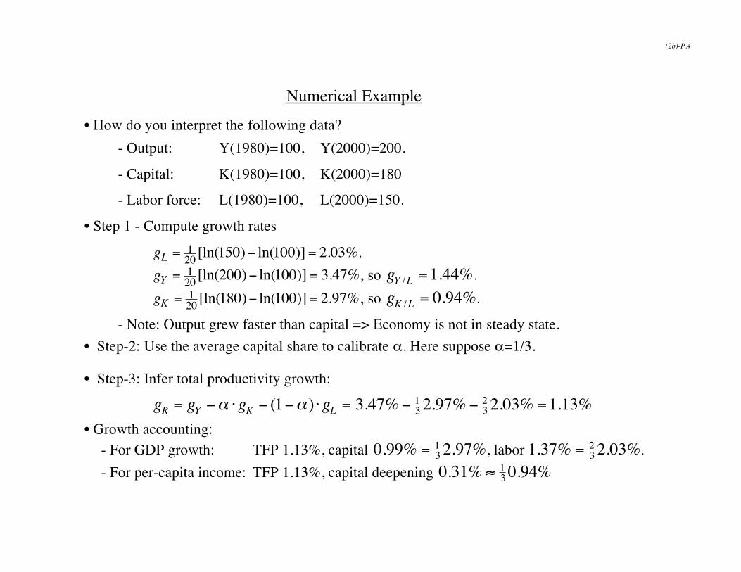
Numerical Example

- Output: Y(1980)=100, Y(2000)=200.

- Capital: K(1980)=100, K(2000)=180

- Labor force: L(1980)=100, L(2000)=150.

- Compute growth rates

gL = 120 [ln(150)− ln(100)] = 2.03%

gY = 120 [ln(200)− ln(100)] = 3.47%

gY /L =1.44%.

gK = 120 [ln(180)− ln(100)] = 2.97%

gK /L = 0.94%.

- Note: Output grew faster than capital => Economy is not in steady state. -2: Use the average capital share to calibrate α α=1/3.

-3: Infer total productivity growth:

gR = gY −α ⋅gK − (1−α ) ⋅gL = 3.47% − 13 2.97% − 2

3 2.03% =1.13%

- For GDP growth: TFP 1.13%, capital

0.99% = 13 2.97%, labor

1.37% = 23 2.03%.

- For per-capita income: TFP 1.13%, capital deepening

0.31% ≈ 13 0.94%

(2b)-P.5

-

Y = f (k) ⋅AL = f (ex ) ⋅AL with

x = ln(k) = ln(K AL)

=>

lnY = ln f (ex ) + lnA + lnL

Note that

ddt ln f (e

x )[ ] =f '(ex )f (ex )

⋅ex =f '(k)f (k) ⋅ k =αk (k)

=>

ddt lnY =αk (k)

d ln kdt + d

dt lnA + ddt lnL

=αk (k)ddt lnK + (1−αk (k))(

ddt lnA + d

dt lnL)

Conclude: Growth accounting relationships always hold for instantaneous growth rates. -

- Cobb-Douglas approximates

α k (k) ≈α ,

(2b)-P.6

- .- s I/Y-

Growth Accounting: Compare TFP levels and growth rates across countries.

Specific questions – separate field: Development (Also miracles & disasters)

(2b)-P.7

R = f '(k) −δ =αk−(1−α ) −δ- -

-

k = K /LA .

If

Ai < Aw , then

(K /L)i < (K /L)w is consistent with

ki = kw .

=> Observed cross-country differences in

(2b)-P.8

δ

.

.

a -

--

[Optional: Acemoglu 3.3.]

- -c-

-

(2b)-P.9

- -

-

-

-

-

-

[

(2b)-P.10

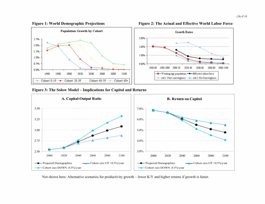
Figure 1: World Demographic Projections Figure 2: The Actual and Effective World Labor Force

Figure 3: The Solow Model – Implications for Capital and Returns

A. Capital-Output Ratio

2.50

2.75

3.00

3.25

3.50

2000 2020 2040 2060 2080 2100

Projected Demographics Cohort size UP +0.5%/year

Cohort size DOWN -0.5%/year

B. Return on Capital

3.0%

4.0%

5.0%

6.0%

7.0%

2000 2020 2040 2060 2080 2100

Projected Demographics Cohort size UP +0.5%/year

Cohort size DOWN -0.5%/year

–

(2b)-P.11

Application III: Natural Resources

-Douglas approach (Romer 1.8, here modified)

- Land T (fixed) and energy E (exhaustible resources) as factor of production, weights β and γ:

Y = Kα ⋅ (AL)1−α −β − γ ⋅T β ⋅Eγ

R(t) = Resource stock at time t, starting with fixed value R(0)

- Resource use: RdtdRE −=−= / = Rate at which the resource is extracted - Define sE = E /R = Share of the resource used in the current period, assumed constant

=> R and E are declining over time: EsEERR −== // [Differs from Romer: here E is productive. But R and E proportional -> same qualitative implications as Romer]

for per-capita income:

y=Y /(AL) = kα ⋅ (T /AL)β ⋅ (E /AL)γ

- Growth accounting =>

gy =α ⋅gk + β ⋅ (−n− g)+ γ ⋅ (gE −n− g)

- On a balanced growth path

gy = gk ,gE = −sE implies

gY /L = gy + g =1−α −β −γ1−α

g− γ1−α

⋅ sE −γ + β1−α

⋅n

1. Fixed resources and land reduce output growth. 2. Per-capita income growth is still possible if g is high enough - Nordhaus: 0.2-0.3% growth reduction - Caveat: Share of energy in factor income has been declining

(2b)-P.12

Learning Objectives

- –-- –Problem sets for practice.

-