applications of laplace transforms instructor: chia-ming tsai electronics engineering national chiao...
TRANSCRIPT

Applications of Laplace Transforms
Instructor: Chia-Ming TsaiElectronics Engineering
National Chiao Tung UniversityHsinchu, Taiwan, R.O.C.

Contents• Introduction
• Circuit Element Models
• Circuit Analysis
• Transfer Functions
• State Variables
• Network Stability
• Summary

Introduction• To learn how easy it is to work with circuits i
n the s domain
• To learn the concept of modeling circuits in the s domain
• To learn the concept of transfer function in the s domain
• To learn how to apply the state variable method for analyzing linear systems with multiple inputs and multiple outputs
• To learn how the Laplace transform can be used in stability analysis
Circuit Element Models
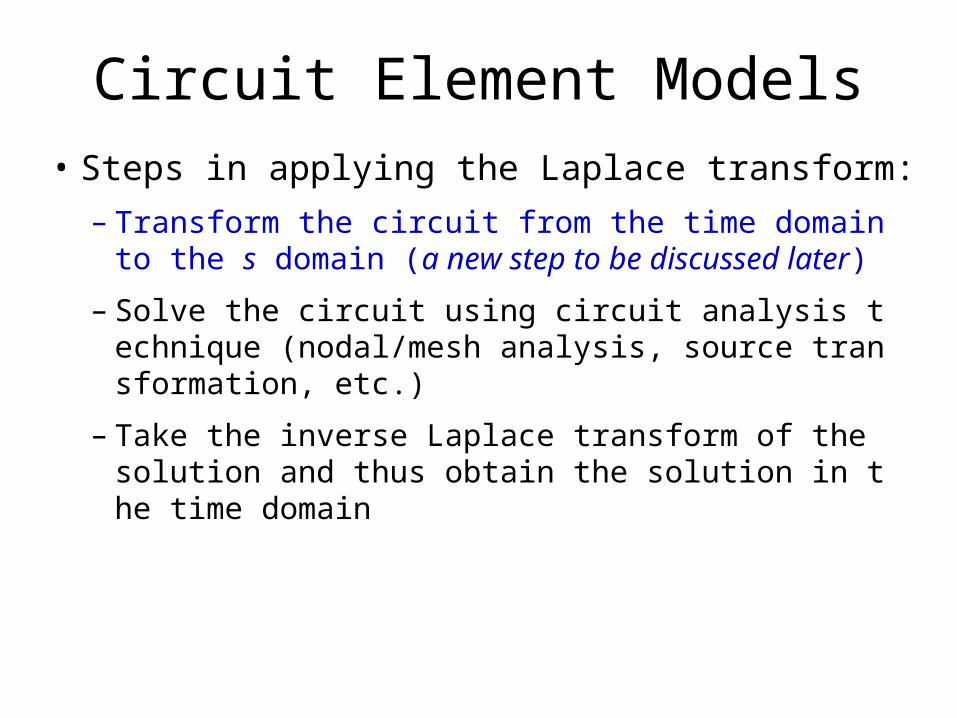
• Steps in applying the Laplace transform:
– Transform the circuit from the time domain to the s domain (a new step to be discussed later)
– Solve the circuit using circuit analysis technique (nodal/mesh analysis, source transformation, etc.)
– Take the inverse Laplace transform of the solution and thus obtain the solution in the time domain

s-Domain Models for R and L
)()(
)()(
)()(
resistor, aFor
sRIsV
tRiLtvL
tRitv
s
isV
sLsI
LissLIissILsV
dt
tdiLtv
)0()(
1)(or
)0()()0()()(
)()(
inductor,an For
Time domain s domain s domain
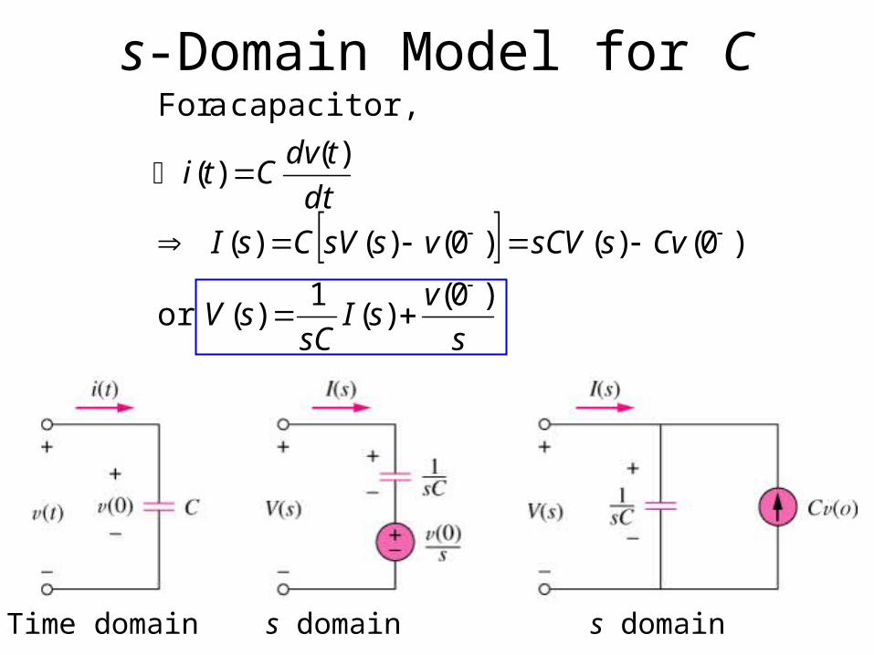
s-Domain Model for C
s
vsI
sCsV
CvssCVvssVCsI
dt
tdvCti
)0()(
1)(or
)0()()0()()(
)()(
capacitor, aFor
Time domain s domain s domain

Summary
s
isV
sLsI
LissLIsV
)0()(
1)(
)0()()(
s
vsI
sCsV
CvssCVsI
)0()(
1)(
)0()()(
For inductor: For capacitor:

Summary
Element Z(s)
Resistor R
Inductor sL
Capacitor 1/sC
*Assuming zero initial conditions
• Impedance in the s domain– Z(s)=V(s)/I(s)
• Admittance in the s domain– Y(s)=1/Z(s)=V(s)/I(s)

Example 1
0 2sin2
3)(
)2()4(
2
2
3
188
3)(
188
3
4
22
22
232
ttetv
s
sssIsV
sssI
to
o
03
53
033
11
: analysismesh Applying (2)
31)F
3
1(
)H 1(
1
)(
:domain thetion toTransforma (1)
21
21
Is
sIs
Is
Iss
ssCZ
ssLZs
tu
s

Example 2
V 5)0( ov

Example 2 (Cont’d)
)()1510(
15)()2(
10)()1(
method, residue theApplying
2
2
1
||
tuee(t)v
sVsB
sVsA
tto
so
so
21)2)(1(
3525
10105.02
10
)1(10
: nodeat analysis nodal Applying
s
B
s
A
ss
sV
s
VVVs
a
o
ooo
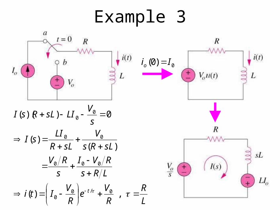
Example 3
0)0( Iio
L
R
R
Ve
R
VIti
LRs
RVI
s
RV
sLRs
V
sLR
LIsI
s
VLIsLRsI
t
, )(
)()(
0))((
0/00
000
00
00

Circuit Analysis
• Operators (derivatives and integrals) into simple multipliers of s and 1/s
• Use algebra to solve the circuit equations
• All of the circuit theorems and relationships developed for dc circuits are perfectly valid in the s domain

Example 1
)(3035)(
2
30
1
35
)2)(1(
540
0)1.0(1
)0()0(
5
0
310
21
1
111
tueetv
ssss
sV
s
svV
s
i
s
VVV
tt
s
V 5)0(
A 1)0(
10
v
is
Vs

Example 2
)(3035
)()101030()51030(
)()()()(
)(105)(
2
10
1
5
)2)(1(
5
)(1010)(
2
10
1
10
)2)(1(
10
)(3030)(
2
30
1
30
)2)(1(
30
:ionsuperposit usingby 1 example Solved
2
2
321
23
3
22
2
21
1
tuee
tuee
tvtvtvtv
tueetv
ssss
sV
tueetv
ssssV
tueetv
ssssV
tt
tt
tt
tt
tt

Example 3Assume that no initial energy is stored.(a)Find Vo(s) using Thevenin’s theorem.(b)Find vo(0+) and vo() by apply the initial- and final-value theorems.(c) Determine vo(t).
=10u(t)

Example 3: (a)
)4(
12550
325
5
5
5
32)32(50
50
)32(
50
2 ,
32
1002
and
02
0
5
0)2(10
:analysis nodal Applying
use , find To
50105
11
1
11
ssssV
ZV
sss
s
I
VZ
sss
VI
sV
s
VI
s
VIV
s
IVZZ
ssVV
ThTh
o
sc
ocTh
x
x
x
scocThTh
Thoc

Example 3: (b), (c)
4
125
4
125lim)(lim)(
gives theoremvalue-final The
04
125lim)(lim)0(
gives theoremvalue-initial The
)4(
125)(
:(b)Solution
00
sssVv
sssVv
sssV
so
so
so
so
o
)()1(25.31)(
25314
125)()4(
25314
125)(
method, residue theApplying
4)4(
125)(
:(c)Solution
4
4
0
tuetv
.sVsB
.ssVA
s
B
s
A
sssV
to
so
so
o
|
|

Transfer Functions• The transfer function H(s) is the ratio of the out
put response Y(s) to the input excitation X(s), assuming all initial conditions are zero.
)( of transformLaplace the:)(
network theof response impulseunit the: )(
impliesIt
)()(or )()( Thus
1)( , )()( If
thsH
th
thtysHsY
sXttx
)()()( , )(
)()( sHsXsY
sX
sYsH

Transfer Functions (Cont’d)• Two ways to find H(s)
– Assume an input and find the output
– Assume an output and find the input (the ladder method: Ohm’s law + KCL)
• Four kinds of transfer functions
)(
)(Admittance)( ,
)(
)(Impedance)(
)(
)(gainCurrent )( ,
)(
)(gain Voltage)(
sV
sIsH
sI
sVsH
sI
sIsH
sV
sVsH
i
o
i
o

Example 1
)( 4sin40)(10)(
4)1(
44010
4)1(
)1(10
)(
)()(
4)1(
)1(10)( ,
1
1)(
:Solution
response. impulse its andfunction transfer theFind
).()( when )( 4cos10)( If
2222
2
22
tutetth
ss
s
sX
sYsH
s
ssY
ssX
tuetxtutety
t
tt

Example 2
)212()4(
)4(
division,current By
:Solution
02 ss
IsI
1122
)4(4
)(
)()(
216
)4(22
20
0
020
ss
ss
sI
sVsH
ss
IsIV
FindH(s)=V0(s)/I0(s).

Example 2 (The Ladder Method)
1122
)4(41)(
)4(4
1122
gives KCL Applying
)4(4
14
4
4
14
4
11
2
12
212 law, sOhm'By
V, 1Let
200
0
2
210
11
21
02
0
ss
ss
II
VsH
ss
ssIII
ss
s
s
VI
s
s
ssIV
VI
V

Example 3Find(a) H(s) = Vo/Vi,(b) the impulse response,(c) the response when vi(t) = u(t) V,(d) the response when vi(t) = 8cos2t V.

Example 3: (a), (b)
i
i
iab
abo
Vs
s
Vss
ss
Vs
sV
Vs
V
32
1
)2()1(1
)2()1(
)1(||11
)1(||11
1
division, By voltage
:Solution
)(5.0)(
23
1
2
1
32
1)(
3232
1
1
1
23 tueth
ssV
VsH
s
VV
s
s
sV
t
i
o
iio

Example 3: (c), (d)
V )(13
1)(
3
1 ,
3
1
23
23
2
1
)()()(
1)()()(
(c):Sol
23 tuetv
BA
s
B
s
A
ss
sVsHsVs
sVtutv
to
io
ii
V )(2sin3
42cos
25
24)(
4
2
3
4
423
1
25
24)(
25
64 ,
25
24 ,
25
24
423
423
4
)()()(4
8)(2cos8)(
(d): Sol
23
22
22
2
tuttetv
ss
s
ssV
CBA
s
CBs
s
A
ss
s
sVsHsVs
ssVttv
to
o
io
ii

State Variables• The state variables are those variables which,
if known, allow all other system parameters to be determined by using only algebraic equations.
• In an electric circuit, the state variables are the inductor current and the capacitor voltage since they collectively describe the energy state of the system.

State Variable Method
s variablestate
ngrepresenti
vectorstate the
)(
)(
)(
)(x
where
BzAxx
as arranged becan equation state The
2
1
n
tx
tx
tx
t
n
DzCxy
BzAxx
)(
)(
)(
)(
)(
)(
x 2
1
2
1
tx
tx
tx
dttdx
dttdx
dttdx
nn
)(
)(
)(
)(z 2
1
tz
tz
tz
t
m
)(
)(
)(
)(y 2
1
ty
ty
ty
t
p

State Variable Method (Cont’d)
DZ(s))BZ(A)IC(
DZ(s))CX()Y(
matrixidentity the:I
)BZ(A)I()X(
)BZ()A)X(I(
)BZ()AX()X(
, transformLaplace theapplying and
conditions initial zero Assuming
DzCxy
BzAxx
1
1
ss
ss
sss
sss
ssss
BAsICsH
sH
sH
D
D
C
B
A
DBAsICsZ
sYsH
1
1
)( )(
.)( ofr denominato
theof degree than theless is )(
ofnumerator theof degree theSo
. 0 cases,most In
matrix feedforwad
matrix output
matrix couplinginput
matrix system
where
)()(
)()(

How to Apply State Variable Method• Steps to apply the state variable method to circ
uit analysis:
– Select the inductor current i and capacitor voltage v as the state variables (define vector x, z)
– Apply KCL and KVL to obtain a set of first-order differential equations (find matrix A, B)
– Obtain the output equation and put the final result in state-space representaion (find matrix C)
– H(s)=C(sI-A)-1B

Network Stability• A circuit is stable if its impulse response h(t) is
bounded as t approaches ; it is unstable if h(t) grows without bound as t approaches .
• Two requirements for stability
– Degree of N(s) < Degree of D(s)
– All the poles must lie in the left half of the s plane
1n if )(lim
)(
)(
)(
)()( If 01
11
th
sD
sRksksksk
sD
sNsH
t
nn
nn
0 ifonly 0)( i
ttjtp iiii eee

Network Stability (Cont’d)• A circuit is stable when all the poles of its tr
ansfer function H(s) lie in the left half of the s plane.
• Circuits composed of passive elements (R, L, and C) and independent sources either are stable or have poles with zero real parts.
• Active circuits or passive circuits with controlled sources can supply energy, and can be unstable.

Example 1
LC
L
R
p
LCLRss
L
sCsLR
sC
V
VsH
s
o
12 where
1
1
1
1)(
0
20
22,1
2
(unstable) 0
:0For
(stable) 0
:0 , ,For
R
CLR

Example 2
sC
kRCsR
sCk
sCsCR
I
I
sCR
sCk
sCsCR
V
kIsC
II
sCR
sC
II
sCRV
i
i
2
111
ist determinan The
11
11
0
01
01
gives analysismesh Applying
2
2
2
1
11
2
21
RkCR
Rkp
CR
Rkp
2
02
operation, stableFor
2
asgiven is pole single the
, 0Let
2
2
Find k for a stable circuit.

Summary• The methodology of circuit analysis using Lapl
ace transform– Convert each element to its s-domain model– Obtain the s-domin solution– Apply the inverse Laplace transform to obtain the
t-domain solution

Summary• The transfer function H(s) of a network is the Lap
lace transform of the impulse response h(t)
• A circuit is stable when all the poles of its transfer function H(s) lie in the left half of the s plane.
)()()( , )(
)()( sHsXsY
sX
sYsH