applications of modified f-expansion method for · pdf fileapplications of modified...

ISSN (e): 2250 – 3005 || Vol, 04 || Issue, 6 || June– 2014 ||

International Journal of Computational Engineering Research (IJCER)

www.ijceronline.com Open Access Journal 5

Applications of Modified F-Expansion Method for Nonlinear

Partial Differential Equations with Variable Coefficients

1,Priyanka M. Patel ,

2,Vikas H. Pradhan

1,2,Department of Applied Mathematics & Humanities, S. V. National Institute of Technology, Surat-395007,

India

I. INTRODUCTION Many phenomena arising in many fields of sciences and engineering have been modeled in modern

times in terms of nonlinear partial differential equations (NLPDEs). As mathematical models of the phenomena,

the study of exact solutions of NLPDEs will help us to understand the underlying mechanism that governs these

phenomena or to provide better knowledge of its physical content and possible applications. Recently, the study

of variable coefficients nonlinear partial differential equations (VC-NLPDEs) has become more and more

attractive. This is because of the fact that a large number of important physical phenomena can be described by

these equations. To find exact solutions of VC-NLPDEs, many powerful methods have been developed such as

the tanh function method [3,10], exp-function method [3,6,13], F-expansion method [9,15], adomain

decomposition method [1], sine-cosine [3] method, extended mapping transformation method [12], '

G G

expansion method [4,5,11] and so on. In the present study, the modified F-expansion method is used to construct

the exact solutions of VC-NLPDEs. As applications of the method, we will consider Burgers’ equation [2] and

BBM equation [14] with variable coefficients.

The plan of the paper is as follows: in section 2, we describe the modified F-expansion method. In section 3, we

construct the exact solutions of Burgers’ equation and BBM equation with variable coefficients. Some

conclusions are given in the last section.

II. INTRODUCTION TO MODIFIED F-EXPANSION METHOD Introduction of modified F-expansion method with constant coefficients is shown in [7,8]. In this study,

we introduce modified F-expansion method with variable coefficients.

Consider a given nonlinear partial differential equation with variable coefficients as:

, , , , , ... 0t x x x x x x

P u u t u t u t u (1)

where ,u x t is the solution of the eq.(1).

The main points of the modified F-expansion method for solving eq.(1) are as follows:

[1]. Using the transformation,

,u x t u where k x v t d t (2)

where 0k is a constant and v t is an integrable function of t .

Substituting eq.(2) into eq.(1) yields an ordinary differential equation for u

' ' 2 '' 3 '''

, , , , , ... 0P u v t u k t u k t u k t u (3)

where prime denotes the derivative with respect to .

ABSTRACT The modified F-expansion method is used to obtain the new exact travelling wave solutions of Burger

equation and Benjamin-Bona-Mahony (BBM) equation with variable coefficients. The obtained solutions

include solitary wave solutions, trigonometric function solutions and rational solutions. In addition some

figures are provided for direct viewing analysis.

KEYWORDS: modified F-expansion method, Burgers’ equation and BBM equation with variable

coefficients, solitary wave solutions, trigonometric function solutions, rational solutions

Applications Of Modified F-Expansion Method…

www.ijceronline.com Open Access Journal Page 16

[2]. Suppose that u can be expressed as

N

i

i

i N

u a F

where 0N

a (4)

where , . . . , 1, 0 ,1, . . . . ,i

a i N N are constants, N is a positive integer which can be determined by

considering the homogeneous balance between the governing nonlinear term(s) and highest order derivatives of

u in eq.(3) and F is a solution of following Riccati equation,

' 2

F A B F C F (5)

where , ,A B C are constants.

[3]. Substitute eq.(4) into eq.(3) and using eq.(5) then left-hand side of eq.(3) can be converted into a finite

series in p

F , , . . . . , 1, 0 ,1, . . . ,p N N . Equating each coefficient of p

F to zero yields a system of

algebraic equations.

[4]. Solve the system of algebraic equations probably with the aid of Mathematica, we obtain the values of

,i

a v t . Substituting these values into eq.(4), we can obtain the travelling wave solutions to eq.(3).

[5]. From the general form of travelling wave solutions listed in appendix, we can give a series of soliton-like solutions, trigonometric function solutions and rational solutions of eq.(1).

III. APPLICATIONS OF THE METHOD 3.1 Variable coefficient Burgers’ equation We consider the variable coefficient Burgers’ equation in the form,

0t x x x

u t u u t u (6)

where t and t are arbitrary functions of t .

Using the transformation,


where 0k is a constant and v is a function of t which is determined later.

Substituting eq.(7) into eq.(6), we get following ordinary differential equation

' ' 2 ''

0v t u k t u u k t u (8)

Now, balancing the orders of '

u u and ''u , we get integer 1N . So we can write solution of eq.(6) in the form,

,u x t u where 1

0 1 1u a a F a F

(9)

where 0 1 1

, ,a a a

are constants and F is a solution of eq.(5).

Inserting eq.(9) together with eq.(5) into eq.(8), the left hand side of eq.(8) can be converted into a finite series

in p

F ,( 3 , 2 , 1, 0 ,1, 2 , 3p ). Equating each coefficient of p

F to zero, we get system of algebraic

equations for 0 1 1, , , ,a a a k v t

.

3 2 2 2

1 1

2 2 2

1 0 1 1 1

1 2 2 2

1 0 1 1 1

2

1

0 2

1 1 0 1 0 1 1

2

1

1

1 0 1

: 2 0

: 3 0

:

2 0

:

0

:

F A k a t A k a t

F A a v t A k a a t B k a t A B k a t

F B a v t B k a a t C k a t B k a t

A C k a t

F C a v t A a v t C k a a t A k a a t B C k a t

A B k a t

F B a v t B k a a t

2 2 2

1 1

2

1

2 2 2

1 0 1 1 1

3 2 2 2

1 1

2 0

: 3 0

: 2 0

A k a t B k a t

A C k a t

F C a v t C k a a t B k a t B C k a t

F C k a t C k a t

(10)

Solving the above algebraic equations with the help of Mathematica, we get the following results

for 0 1 1, , ,a a a v t

.



Case 1: 0A , we have

2

0 1

0 0 1 1 1

1 1

2 2, 0 , , ,

k C a B a t C k ta a a a a v t t

a a

(11)

Case 2: 0B , we have

2

0

0 0 1 1 1

1 1

2 2, 0 , , ,

C k a t C k ta a a a a v t t

a a

(12)

2

01

0 0 1 1 1

1 1

2 2, , , ,

C k a t C k tA aa a a a a v t t

C a a

(13)

Case 3: 0A B , we have

2

0

0 0 1 1 1

1 1

2 2, 0 , , ,

C k a t C k ta a a a a v t

a a

(14)

Substituting these results into eq.(9) and using appendix, we obtain the following travelling wave solutions of

eq.(6).

(1) Select 0 , 1, 1A B C and 1 1

ta n h2 2 2

F

from appendix and using eq.(11), we get

2

0 1

1 0 1

1

21 1 1, ta n h

2 2 2

k a a t d t

u x t a a k xa

(15)

(2) Select 0 , 1, 1A B C and 1 1

c o th2 2 2

F


2

0 1

2 0 1

1

21 1 1, c o th

2 2 2

k a a t d t

u x t a a k xa

(16)

(3) Select 1 1

, 0 ,2 2

A B C and c o th c s c ,F h

ta n h s e ci h from appendix and using eq.(12) and eq.(13) respectively, we get

2 2

0 0

3 0 1

1 1

, c o th c s c

k a t d t k a t d t

u x t a a k x h k xa a

(17)

12 2

0 0

4 0 1

1 1

2 2

0 0

1

1 1

, c o th c s c

c o th c s c

k a t d t k a t d t

u x t a a k x h k xa a

k a t d t k a t d t

a k x h k xa a

(18)

2 2

0 0

5 0 1

1 1

, ta n h s e c

k a t d t k a t d t

u x t a a k x i h k xa a

(19)

12 2

0 0

6 0 1

1 1

2 2

0 0

1

1 1

, ta n h s e c

ta n h s e c

k a t d t k a t d t

u x t a a k x i h k xa a

k a t d t k a t d t

a k x i h k xa a

(20)

(4) Select 1, 0 , 1A B C and ta n h , c o thF from appendix and using eq.(12), eq.(13)

respectively, we get



2

0

7 0 1

1

2

, ta n h

k a t d t

u x t a a k xa

(21)

12

0

8 0 1

1

2

0

1

1

2

, ta n h

2

ta n h

k a t d t

u x t a a k xa

k a t d t

a k xa

(22)

2

0

9 0 1

1

2

, c o th

k a t d t

u x t a a k xa

(23)

12

0

1 0 0 1

1

2

0

1

1

2

, c o th

2

c o th

k a t d t

u x t a a k xa

k a t d t

a k xa

(24)

(5) Select 1 1

, 0 ,2 2

A B C and s e c ta n , c s c c o tF from appendix and using eq.(12),

eq.(13) respectively, we get

2 2

0 0

1 1 0 1

1 1

, s e c ta n

k a t d t k a t d t

u x t a a k x k xa a

(25)

12 2

0 0

1 2 0 1

1 1

2 2

0 0

1

1 1

, s e c ta n

s e c ta n

k a t d t k a t d t


k a t d t k a t d t

a k x k xa a

(26)

2 2

0 0

1 3 0 1

1 1

, c s c c o t

k a t d t k a t d t


(27)

12 2

0 0

1 4 0 1

1 1

2 2

0 0

1

1 1

, c s c c o t

c s c c o t

k a t d t k a t d t


k a t d t k a t d t

a k x k xa a

(28)

(6) Select 1 1

, 0 ,2 2

A B C and s e c ta n , c s c c o tF from appendix and using

eq.(12), eq.(13) respectively, we get

2 2

0 0

1 5 0 1

1 1

, s e c ta n

k a t d t k a t d t


(29)



12 2

0 0

1 6 0 1

1 1

2 2

0 0

1

1 1

, s e c ta n

s e c ta n

k a t d t k a t d t


k a t d t k a t d t

a k x k xa a

(30)

2 2

0 0

1 7 0 1

1 1

, c s c c o t

k a t d t k a t d t


(31)

12 2

0 0

1 8 0 1

1 1

2 2

0 0

1

1 1

, c s c c o t

c s c c o t

k a t d t k a t d t


k a t d t k a t d t

a k x k xa a

(32)

(7) Select 1, 0 , 1A B C and ta nF from appendix and using eq.(12), eq.(13) respectively, we get

2

0

1 9 0 1

1

2

, tan

k a t d t

u x t a a k xa

(33)

12

0

2 0 0 1

1

2

0

1

1

2

, ta n

2

ta n

k a t d t

u x t a a k xa

k a t d t

a k xa

(34)

(8) Select 1, 0 , 1A B C and c o tF from appendix and using eq.(12), eq.(13) respectively, we

get

2

0

2 1 0 1

1

2

, co t

k a t d t

u x t a a k xa

(35)

12

0

2 2 0 1

1

2

0

1

1

2

, c o t

2

c o t

k a t d t

u x t a a k xa

k a t d t

a k xa

(36)

(9) Select 0 , 0 , 0A B C and 1

FC m


2

1

2 3 0 2 2

1 0 1

,

2

au x t a

C k a x C k a t d t a m

(37)

where m is an arbitrary constant.

Graphical presentation:

For the graphical presentation, we taking solution 1,u x t given by eq.(15) as an example. For simplicity we set

0 11, 1a a and

1

2k . Here we plot solution 1

,u x t for different values

of , s in , ta n ht

t a e b t c t .



(a)

tt e

(b) s int t

(c) ta n ht t

Figure 1. Solution of Burgers’ equation with variable coefficients in different form

3.2 Variable coefficient BBM equation

We consider following variable coefficient BBM equation

0p

t x x x x tu a t u b t u u u (38)

where 0p and a t , b t are arbitrary functions of t .

For simplicity here we consider 1p

0t x x x x t

u a t u b t u u u (39)

Taking the transformation,


where 0k and v is a function of t which is determined later.

Substituting eq.(40) into eq.(39), we get ordinary differential equation

' ' ' 2 '''

0v t u k a t u k b t u u k v t u (41)

Balancing the orders of '

u u and '''u , we get integer 2N . So we can write solution of eq.(39) in the form,

2 1 2

0 2 1 1 2u a a F a F a F a F

(42)

Substituting eq.(42) together with eq.(5) into eq.(41), the left hand side of eq.(41) can be converted into a finite

series in p

F ,( 5 , 4 , 3 , 2 , 1, 0 ,1, 2 , 3 , 4 , 5p ). Equating each coefficient of p

F to zero, we get

system of algebraic equations for 0 2 1 1 2, , , , , ,a a a a a k v t

.



5 2 3 2

2 2

4 2 2 2 3 2

2 2 1 2 1

3 2

2 0 2 2 2 1

2 2 2 2 2

1 2 2 2

2 2

1

2

2

: 2 2 4 0

: 2 3 5 4 6 0

: 2 2 2 3

2 3 8 4 0

1 2 0

: 2

F A b t k a A k a v

F b t B k a A b t k a a A B k a v t A k a v t

F a t A k a A b t k a a b t C k a b t B k a a

A b t k a A a v t A B k a v t A C k a v t

A B k a v t

F a t B k a

0 2 1 0 1 2 1

2 3 2 2

1 2 1 2 2 2

2 2 2 2

1 1 1

1 2

2 0 2 1 0 1 1

2

2 1 2

2 3

2 8 5 2

7 8 0

: 2 2

2 1 4

b t B k a a a t A k a A b t k a a b t C k a a

b t B k a A b t k a a B a v t B k a v t A B C k a v t

A a v t A B k a v t A C k a v t

F a t C k a b t C k a a a t B k a B b t k a a b t C k a

b t B k a a C a v t B

2 2 2

2 2 1

3 2 2

1 1

0 2 2

1 0 1 1 0 1 2 1 2

2 2 2 2 2 2 2 2

1 1 1 1 1 1

2 2

1 2 2

1

1 6

8 0

: 6

2 2

6 0

:

C k a v t A C k a v t B a v t

B k a v t A B C k a v t

F a t C k a b t C k a a a t A k a A b t k a a b t C k a a B C k a v t

C a v t B C k a v t A C k a v t A a v t A B k a v t A C k a v t

A b t k a a A B k v t a

F a t B k

2 3 2 2

1 0 1 1 1 1 1 2

2 2 2 2

0 2 1 2 2 2 2

2 2 2 2 2 2

1 0 1 1 1 1 1

2 0 2 1 2 1 2

8 2

2 2 1 4 1 6 0

: 7 8

2 2 3

a B b t k a a A b t k a B a v t B k a v t A B C k a v t a t A k a

A b t k a a b t B k a a A v t a A B k a v t A C k a v t

F a t C k a C b t k a a B b t k a C a v t B C k a v t A C k a v t

a t B k a b t B k a a b t C k a a A b t k a a

3 2

2 2

2

2

3 2 2 2

1 1 2 0 2 1 2 2

2 2 2 2 2

2 2 2

4 3 2 2 2 2

1 1 2 2 2

5 3 2 2

2 2

2 8

5 2 0

: 1 2 2 2 3 2

3 8 4 0 2 0

: 6 3 5 4 2 0

: 2 4 2 0

B v t a B k v t a

A B C k v t a

F b t C k a B C k a v t a t C k a b t C k a a b t B k a a C v t a

B C k v t a A C k v t a A b t k a

F C k a v t b t C k a a B C k a v t b t B k a

F C k a v t b t C k a

(43) Solving above algebraic equations with the help of Mathematica, we obtain following results:

Case 1: 0A , we have

11

0 0 2 1 1 1 2

2 2 2

0 1 1

2

, 0 , 0 , , , ,1 2

1 2

1 2

b t aC aa a a a a a a v t

B B C k

b t B C k a b t a b t B k aa t

B C k

(44)

Case 2: 0B , we have

2

0 0 2 1 1 2 2 2

2 2 2

0 2 2

2 2

, 0 , 0 , 0 , , ,1 2

1 2 8

1 2

b t aa a a a a a a v t

C k

b t C k a b t a b t A C k aa t

C k

(45)

2

22

0 0 2 1 1 2 22 2

2 2 2

0 2 2

2 2

, , 0 , 0 , , ,1 2

1 2 8

1 2

b t aA aa a a a a a a v t

C C k

b t C k a b t a b t A C k aa t

C k

(46)

Case 3: 0A B , we have



2

0 0 2 1 1 2 2 2

2 2

0 2

2 2

, 0 , 0 , 0 , , ,1 2

1 2

1 2

b t aa a a a a a a v t

C k

b t C k a b t aa t

C k

(47)

Substituting these results into eq.(42) and using appendix, we obtain the travelling wave solutions of eq.(39) as

follows:

(1) Select 0 , 1, 1A B C and 1 1

ta n h2 2 2

F


2

11

1 0,

4 2 2 4

a b t d ta k xu x t a s e c h

k

(48)

(2) Select 0 , 1, 1A B C and 1 1

c o th2 2 2

F


2

11

2 0, c s c

4 2 2 4

a b t d ta k xu x t a h

k

(49)

(3) Select 1 1

, 0 ,2 2

A B C and c o th c s c ,F h

ta n h s e ci h from appendix and using eq.(45) and eq.(46) respectively, we get

2

2 2

3 0 2, c sc c o th

3 3

b t a b t au x t a a h k x d t k x d t

k k

(50)

2

2 2

4 0 2

2

2 2

2

, c s c c o th3 3

c sc c o th3 3

b t a b t au x t a a h k x d t k x d t

k k

b t a b t aa h k x d t k x d t

k k

(51)

2

2 2

5 0 2, ta n h se c h

3 3

b t a b t au x t a a h k x d t i k x d t

k k

(52)

2

2 2

6 0 2

2

2 2

2

, ta n h se c h3 3

ta n h se c h3 3

b t a b t au x t a a h k x d t i k x d t

k k

b t a b t aa h k x d t i k x d t

k k

(53)

(4) Select 1, 0 , 1A B C and ta n h , c o thF from appendix and using eq.(45) and eq.(46)


2

2

7 0 2, ta n h

1 2

b t au x t a a k x d t

k

(54)

2

2

8 0 2

2

2

2

, ta n h1 2

ta n h1 2


k

b t aa k x d t

k

(55)

2

2

9 0 2, c o th

1 2


k

(56)



2

2

1 0 0 2

2

2

2

, c o th1 2

c o th1 2


k

b t aa k x d t

k

(57)

(5) Select 1 1

, 0 ,2 2

A B C and s e c ta n , c s c c o tF from appendix and using eq.(45)

and eq.(46) respectively, we get

2

2 2

1 1 0 2, s e c ta n

3 3

b t a b t au x t a a k x d t k x d t

k k

(58)

2

2 2

1 2 0 2

2

2 2

2

, s e c ta n3 3

se c ta n3 3


k k

b t a b t aa k x d t k x d t

k k

(59)

2

2 2

1 3 0 2, c sc c o t

3 3


k k

(60)

2

2 2

1 4 0 2

2

2 2

2

, c s c c o t3 3

c sc c o t3 3


k k


k k

(61)

(6) Select 1 1

, 0 ,2 2

A B C and s e c ta n , c s c c o tF from appendix and using

eq.(45) and eq.(46) respectively, we get

2

2 2

1 5 0 2, s e c ta n

3 3


k k

(62)

2

2 2

1 6 0 2

2

2 2

2

, s e c ta n3 3

se c ta n3 3


k k


k k

(63)

2

2 2

1 7 0 2, c sc c o t

3 3


k k

(64)

2

2 2

1 8 0 2

2

2 2

2

, c s c c o t3 3

c sc c o t3 3


k k


k k

(65)

(6) Select 1 1 , 0 , 1 1A B C and ta n , c o tF from appendix and using eq.(45) and eq.(46)


2

2

1 9 0 2, ta n

1 2

b t au x t a a k x

k

(66)

2 2

2 2

2 0 0 2 2, ta n ta n

1 2 1 2

b t a b t au x t a a k x a k x

k k

(67)



2

2

2 1 0 2, c o t

1 2

b t au x t a a k x

k

(68)

2 2

2 2

2 2 0 2 2, c o t c o t

1 2 1 2

b t a b t au x t a a k x a k x

k k

(69)

(7) Select 0 , 0A B C and 1

FC m


2

2 3 0 2

2

2

1,

1 2

u x t a ab t a

C k x d t mC k

(70)

where m is an arbitrary constant.

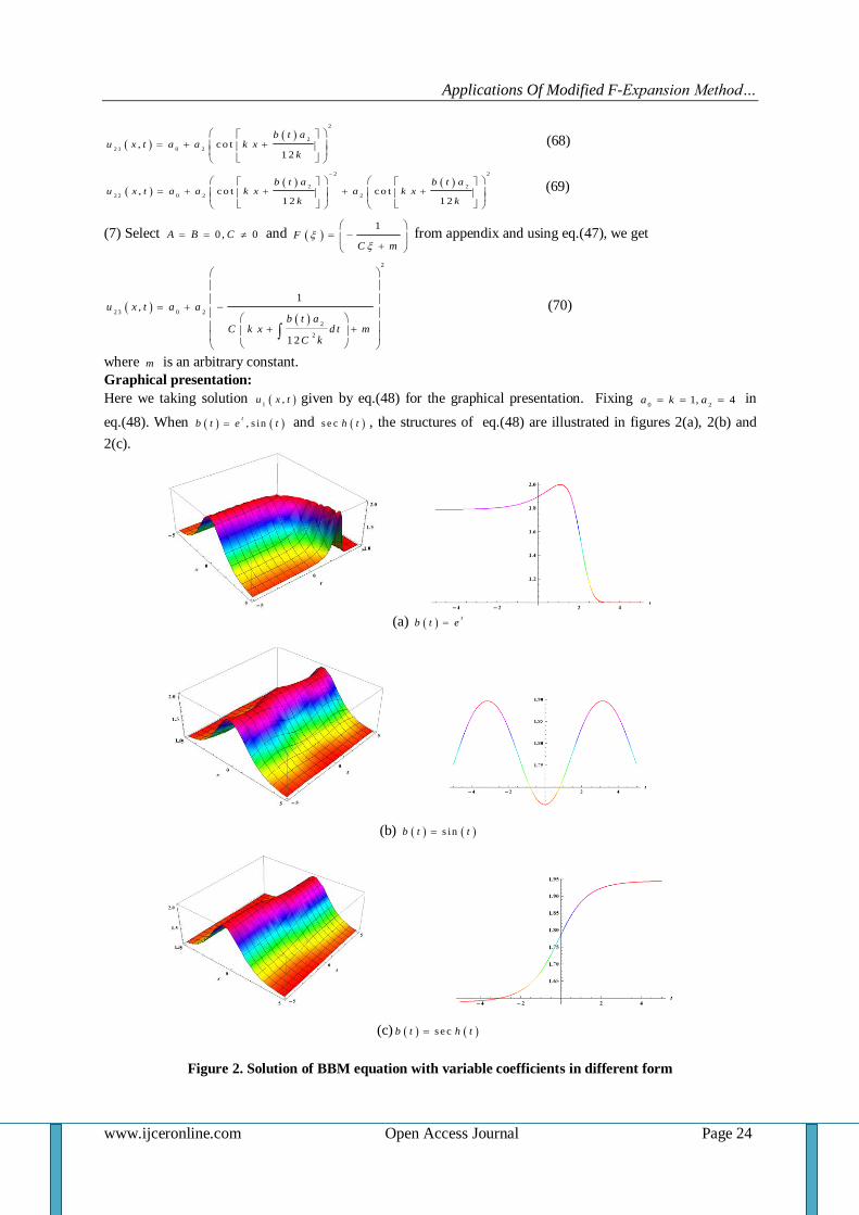
Graphical presentation:

Here we taking solution 1,u x t given by eq.(48) for the graphical presentation. Fixing

0 21, 4a k a in

eq.(48). When , s int

b t e t and s e c h t , the structures of eq.(48) are illustrated in figures 2(a), 2(b) and

2(c).

(a)

tb t e

(b) s inb t t

(c) s e cb t h t

Figure 2. Solution of BBM equation with variable coefficients in different form



IV. CONCLUSION In this paper, exact travelling wave solutions of the Burgers’ equation and BBM equation with variable

coefficients have been obtained using the modified F-expansion method. These solutions are expressed in terms

of hyperbolic, trigonometric and rational functions with arbitrary parameters. The obtained solutions may be useful to further understand the variable coefficients Burger equation and BBM equation and mechanism of the

physical phenomena. The modified F-expansion method is promising and powerful method for handling other

nonlinear partial differential equations with variable coefficients arising in mathematical physics.

Appendix: Relations between values of ( , ,A B C ) and corresponding F in Riccati equation

' 2

F A B F C F

A B C F

0 1 1 1 1

ta n h2 2 2

0 1 1 1 1

c o th2 2 2

1

2 0

1

2 c o th c s c , ta n h s e ch i h

1 0 1 ta n h , c o th

1

2 0

1

2 s e c ta n , c s c c o t

1

2 0

1

2 s e c ta n , c s c c o t

1 1 0 1 1 ta n , c o t

0

0 0

1

m is a n a rb i tra ry c o n s ta n tC m

REFERENCES

[1] A-M. Wawaz, A. Gorguis, “Exact solutions for heat-like and wave-like equations with variable

coefficients”, Applied mathematics and computation, 149(1), pp.15-29, 2004

[2] B. A. Malomed, V. I. Shrira, “Soliton caustics”, Physica D: nonlinear phenomena, 53(1), pp.1-12, 1991

[3] E. M. E. Zayed and M. A. M. Abdelaziz, “Exact solutions for the nonlinear Schrödinger equation with

variable coefficients using the generalized extended tanh-function, the sine-cosine and the exp-function

methods”, Applied mathematics and computation, 218, pp. 2259-2268, 2011

[4] E. M. E. Zayed and M. A. M. Abdelaziz, “Exact travelling wave solutions of nonlinear variable-

coefficients evolution equations with forced terms using the generalized '

G G expansion method”,

Computational mathematics and modeling, 24(1), pp. 103-113, 2013

[5] E. M. E. Zayed, “Exact travelling wave solutions for a variable-coefficient generalized dispersive water-

wave system using the generalized '

G G -expansion method”, Mathematical science letters-an

international journal, 3(1), pp. 9-15, 2014

[6] F. Khani, S. Hamedi-Nezhad, “Some new exact solutions of the (2+1)-dimensional variable coefficient

Broer-Kaup system using the exp-function method”, Computers and mathematics with applications, 58,

pp.2325-2329, 2009

[7] G. Cai and Q. Wang, “ A modified F-expansion method for solving nonlinear pdes”, Journal of

information and computing science, 2(1), pp. 3-16, 2007

[8] G. Cai et al., “A modified F-expansion method for solving breaking soliton equation”, international

Journal of nonlinear science, 2(2), pp. 122-128, 2006

[9] J-F Zhang et al., “Variable coefficient F-expansion method and its application to nonlinear Schrödinger equation”, Optics communications, 252(4-6), pp. 408-421, 2005



[10] L. Wei, “New exact solutions to some variable coefficients problems”, Applied mathematics and

computation, 217(4), pp.1632-1638, 2010

[11] M. A. Abdou et al., “New exact travelling wave solutions of nonlinear evolution equations with variable

coefficients”, Studies in nonlinear sciences, 1(4), pp. 133-139, 2010

[12] M. S. Abdel Latif, “Some exact solutions of kdv equation with variable coefficients”, Communications in

nonlinear science and numerical simulation, 16(4), pp. 1783-1786, 2011

[13] S. Zhang, “Application of exp-function method to a kdv equation with variable coefficients”, physics letters A, 365(5-6), pp.448-453, 2007

[14] V. Bisognin, G. Perla Menzala, “Asymptotic behaviour of nonlinear dispersive models with variable

coefficients ”, Annali di matematica pure ed applicata, 168(1), pp. 219-235, 1995

[15] Y. Zhou et al., “Periodic wave solutions to a coupled kdv equations with variable coefficients”, Physics

letters A, 308(1), pp. 31-36, 2003

applications of modified f-expansion method for · pdf fileapplications of modified...

Documents