applications of multibeam water column imaging for ... of multibeam water column imaging for...

Hughes Clarke 1 Multibeam water column imaging

Applications of multibeam water column imaging for hydrographic survey.

John E. Hughes Clarke Ocean Mapping Group

Dept. Geodesy and Geomatics Engineering University of New Brunswick

P.O. Box 4400, Fredericton, NB, E3B 5A3, Canada [email protected]

Abstract Water column imaging multibeam sonars are just now becoming widely available to the hydrographic community. Whilst originally developed to serve the fisheries community, this added functionality provides several significant advantages to the hydrographer in quality control. In order to interpret the spatial patterns of echoes within the approximately two-dimensional cross-section for each ping, a complete understanding of the role of sidelobes, sectors and seabed angular response is needed. This paper reviews the imaging geometry, provides synthetic examples of the echo character of typical seafloors, and then goes on to examine real examples of mid water returns that impact on the quality of hydrographic data. Examples include interference from other sonars, propeller and engine noise, bubble wash-down, bottom detection failures, false tracking on wreck-like targets, and natural thermocline and fish targets. Each example is explained to show how, with proper interpretation, increased confidence in the validity of spurious soundings or echoes may be obtained. It is predicted that, in the near future, these data types will be routinely incorporated in the hydrographic quality control data stream. They provide both increased confidence in the sounding data quality as well as timely indicators of the imminent decline in image quality. Furthermore, the data can provide a value-added product for the fisheries and oceanographic imaging community. Introduction Acoustic imaging of the water mass and its contents using angle-discriminating sonars is not new. Multibeam sonars, adapted for mid-water imaging, have been available to the fishing community for many years. The Simrad SM600, SR240, SP270 and SA950 sonars were all designed to image within the hemisphere below the vessel using steered beams with beam widths of about 12°. Examples of their use for scientific applications include: Misund and Aglen, (1992), Misund, (1993), Hafsteinsson and O. A. Misund, (1995). Forward-looking imaging multibeams that use a broad transmit (20+°) but with narrow 1.5° beams were also adapted for water column imaging. These included the RESON

The Hydrographic Journal 1 April, 2006

mailto:[email protected]


6012 (455 kHz, a version of which, with a 1.5° transit, became the well known 9001) and the Mesotech SM2000 (which also has an option of a 1.5° transmit for narrower beam applications). Examples of their use for imaging include: Gerlotto et al.(1994, 1999), Soria et al.,(1996), Nøttestad and B. E. Axelsen (1999), Axelsen et al., (2001) and Benoit-Bird and W. Au, 2003. Once the potential of imaging multibeams had been demonstrated, research turned toward improved visualization techniques (Mayer et al., 2002) and most recently calibrating the return to attempt biomass quantification (Cochrane et al. 2003, Foote et al., 2005). Applications beyond fisheries imaging have been attempted including imaging bubble populations (Weber et al., 2003, using a RESON 8101), measuring suspended particulate density (Jones, 2003, using an SM2000), and military mid-water target hunting (Gallaudet and deMoustier, 2003). Almost all the applications described above used data at ranges shorter than the distance of closest approach to the seafloor. Thus bottom related echoes did not contaminate the water column imagery. In contrast, multibeam sonars used in the hydrographic industry are primarily adapted to extracting echoes about the bottom. This makes the imagery much harder to interpret, yet provides new information about the bottom and near bottom targets. Principles of Water Column Imaging Water Column imaging can be achieved from a wide range of multibeam-like geometries. The ones used as examples herein (the Kongsberg EM710 and EM3002 sonars) are optimized for seabed interaction. Specifically the dynamic range of the receivers and the gain settings are designed not to saturate with typical bottom backscattered intensities. In addition beam widths are narrow to best attempt spatial resolution of bottom morphology. It should be noted that the water column imaging method described herein can only be applied to systems using narrow receive beams. Differential phase bathymetric systems (often referred to as interferometric) cannot generate a meaningful water column image because there are no methods to discriminate the angle relationship of multiple echoes that occur at a fixed time. The usual methodology relies on assuming a single angle solution at a given slant range. Even refinements to the interferometric method, such as the SARA/CAATI algorithm (Krautner and Bird, 1995) still only allow up to 3 solutions at a given slant range. All the images shown are presented in one of two ways : Time-Angle Space (Fig. 1, top left): fundamentally, multibeam sonars are angle-time discriminating systems. For conventional beamforming, a series of preformed beams listen along intended sonar-referenced or vertically-referenced angles. For FFT beamformers the reverse is true: for a given time, a series of angle bins are examined. For either approach, the echo intensities can be mapped in a two-dimensional image space



with angle on one axis and time on the other. Under this representation, a flat seafloor appears as a parabolic trace. Depth-Across Track Space (Fig. 1 bottom): Ultimately, for topographic imaging, the echo intensity field has to be remapped into the approximately two-dimensional near-vertical plane under the vessel. This involves a transformation from polar coordinates to cartesian. Complications in this transformation can occur due to irregular or uneven beam spacing. Refracted ray paths and the along track distortion of the transmit beam pattern due to pitch and pitch steering must also be taken into account. This plot is familiar to users of the RESON Seabat family of sonars. A real-time, sonar-referenced display of the polar intensity plot has always been available as an intuitive source of quality control. The advances in imaging, described herein, reflect proper registration of those images and most significantly, the ability to retain the information for post-acquisition analysis. One should note also that the RESON displays were generally colour or greyscale coded by linear intensity. Herein, the greyscale in the images corresponds to logarithmic intensity. Linear intensity displays are better for looking at the peak intensities normally associated with just the mainlobe bottom interaction. The logarithmic images will show better the weaker echoes associated with water column scatterers and sidelobe contributions.



Fig. 1: Illustrating the alternate modes of presenting acoustic intensity information from a multibeam sonar. Top-left: Time-Angle representation. Top-right : conceptual imaging geometry. Bottom: Depth –

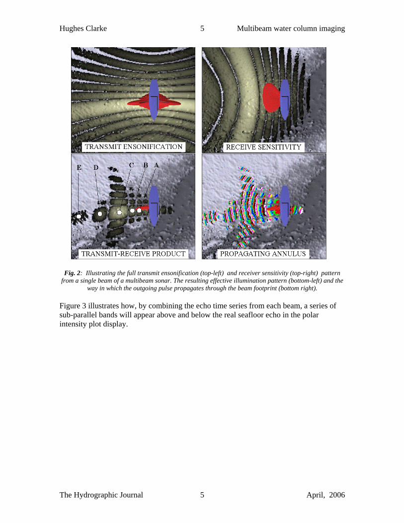
Across Track distance representation (polar plot). It is important to appreciate that intensities are mapped to the angle of the principal response axis of any particular beam. Depending on the level of sidelobe suppression for that beam, the echoes received may or may not actually lie at that angle. Before looking at the images, it is important to understand the imaging geometry, the effect of sidelobes, sectors and angular responses on the water column imagery. Receiver Sidelobe Contributions The most fundamental issue to realize is that the plot is constructed radially of time series along each intended beam azimuth. Any beam, of course, has some sensitivity outside its maximum response axis (the beam boresite). The pattern of sidelobes for conventional Mills Cross beams is a result of the interaction of the main and side lobes of the transmit beam (Fig. 2, top-left) and those of the receiver channel (Fig. 2, top-right) for that beam. When the transmit and receive beam patterns are multiplied together, the projected product, represents a series of semi-elliptical footprints lying primarily along the axes of the two main lobes (Fig. 2, bottom left) The strongest seabed echo should normally be received from the central mainlobe-mainlobe intersection (Fig. 2 bottom left, C). However, as the pulse annulus propagates through this ensonification pattern (Fig. 2 bottom right), a series of echoes will be received both before and after the main echo. These are usually unimportant for the purposes of tracking a low-relief seafloor. But when looking for mid-water scatterers or in the presences of rapid changes in slope, they have a great potential to cause confusion. All beams away from nadir will pick up a sequences of echoes inboard of the boresite, including the near specular first arrival. All of this must be accounted for in interpreting the polar intensity plots.



Fig. 2: Illustrating the full transmit ensonification (top-left) and receiver sensitivity (top-right) pattern from a single beam of a multibeam sonar. The resulting effective illumination pattern (bottom-left) and the

way in which the outgoing pulse propagates through the beam footprint (bottom right). Figure 3 illustrates how, by combining the echo time series from each beam, a series of sub-parallel bands will appear above and below the real seafloor echo in the polar intensity plot display.



Fig. 3: Subset of the polar plot display with receiver beam pattern superimposed. The location of the bottom strike of each of the main and side lobes is indicated by the white arrowed line and the black dot.

Each dot is indicated by a letter that corresponds to the illumination maxima indicated in Figure 2 (lower left). Because, within a single beam, one cannot tell which lobe is responding, all intensity information reported for that beam is plotted along the beam boresite direction. The end result is a series of bottom

near-parallel bands that lie above and below the real seafloor mainlobe echo. As a result of the presence of the sidelobes, seabed echoes will contaminate the water column data at any slant range beyond that of the closest distance of approach to the seabed. As a result, water column echoes are best viewed within a semi-circle of radius equal to the minimum slant range to the seafloor (Fig. 3). How severe the contamination of the water column signature is will depend on the level of sidelobe suppression and the nature of the bottom backscatter strength of the seafloor. A particularly important component is the way in which the seabed backscatter strength varies with grazing angle, herein termed the angular response. Angular Response Signature If the seabed backscatter strength did not vary with grazing angle, the echo from the first arrival (which is normally specular) would not be nearly so noticeable. The echo would still be stronger than for oblique angles because the ensonified area (controlled by the projected pulse length) is locally a maximum at nadir. For typical multibeam hardware, sidelobe suppression of about 25 dB is normally achieved. However, vertical incidence



backscatter strength of typical seafloors usually is 5 to 20 dB stronger than for oblique echoes. As a result the first arrival is normally almost as strong as the echo from the main lobe seafloor intersection. Echoes in the water column beyond the first arrival, are contaminated by seabed sidelobe echoes whose contribution will depend on the bottom backscatter strength at that slant range. Despite this contamination, water-column target detection beyond the minimum slant range to the seafloor may still be achieved on low backscatter strength seabeds. Local fluctuations in the apparent scattering in the water column will however, be in part controlled by variations in the seabed backscatter strength and grazing angle at that equivalent slant range. Thus we need to understand the influence of off-track topography. Effect of Off-Track Topography. For benign seafloors, the bottom backscatter strength will decrease markedly at ranges away from normal incidence. However, more dynamic topography may present inward facing slopes, where, in extreme geometries (e.g.: man-made structures or consolidated seabeds such as bedrock outcrop or coral reefs), a near-specular echo can be achieved, thereby strongly contaminating the water column imaging. To illustrate this, a synthetic polar intensity image has been generated (Fig. 4) that shows the effect of a periodic undulation in the seafloor. The seafloor model has a strong angular response signature, and thus, as the undulations slope in toward the receiver, the echo intensity rises. The importance of this depends on the beam angle. At angles close to nadir, small undulations in the seafloor can produce specular signatures. At angles further out, it is harder to achieve specular echoes, but easier to cast shadows. In figure 4, one can observe that, each time a specular echo is generated, a fixed range arc of high intensity appears in the image, potentially contaminating the water column imagery.



Fig.4: Synthetic water column image generated for the case of a gently undulating seafloor. Indicating the resulting water-column image (polar plot) with the location of specular echoes and shadows shown.

Point scatterers and local specular facets, such as are common on wreck-like objects, will produce an arcuate series of false echoes in the water column at the equivalent slant range. Under these circumstances it is far harder to confidently pick out other weaker water column scatterers at the same slant range but different elevation angles. This is very common in the presence of boulder-like targets. The synthetic model presented in figure 5 illustrates the effect. The inward facing slope of the boulders will tend to be specular and generate a range arc of high intensity echoes that can potentially distort the bottom tracking, providing solutions both above and below the true boulder position.



Fig. 5: Synthetic water-column image generated for the case of a flat seafloor with intersperse 2m radius hemispheres. Indicating the resulting water-column image (polar plot) with the location of specular echoes

and shadows shown. WMT – weighted mean time bottom detection. In the models shown, only the two-dimensional, across track slope is considered and only the main lobe of the transmitter is considered. In reality, the full three dimensional seafloor slope must be accounted for. If the seafloor slopes along track as well, there may be no true specular echo in the recorded time series. As well as the main lobe of the transmit beam pattern, however, one needs to be aware that significant contributions can also come from sidelobes of the transmitter. Transmit Sidelobe Contributions. Should there be a specular geometry ahead or behind the vessel, or a region of particularly strong scattering that lies within the transmit sidelobes (Fig. 2 top_left), a ghost-like echo will appear in the water-column imaging before the main lobe reaches the target of interest. To illustrate this phenomena, three water-column images from an EM3002 are presented as one steams obliquely across a wreck (Fig. 6). As well as the main-lobe tracking on the wreck itself, one clearly sees a ghost-like echo indicating the upcoming wreck (top figure) and the wreck after it has been passed over (lower figure). The ghost is a result of the wreck lying within the transmit sidelobe footprint. At those times, the seabed echo is still very clear as it lies under the main lobe. As will be explained later, echoes from



small proud objects around and above the wreck such as masts are of great concern. If the bottom track algorithm is altered to track these weaker echoes, one runs the risk of locking on to these ghost echoes as well.

Fig. 6: Three water column images generated using an EM3002 over a wreck. The wreck is traversed

obliquely(steaming from SW to NE) so that not all the wreck ever lies in the transmit main lobe at any one time. The imagery, however, clearly indicates that a contribution from the wreck is still visible from energy

transmitted from the sidelobes of the transmitter. Data from CSL Heron. Multiple Transmit Sectors As described above, for single-ping-ensonification systems (such as the EM3002), the first arrival echo, received through the sidelobes will practically limit the maximum slant range within which confident mid-water target recognition can be achieved. One way to get around the problem of the first arrival is to break up the sector into 3 or more discrete pings using non-overlapping frequency ranges. In this manner, the outer sector transmit beams patterns can be designed to have a null close to vertical incidence, so that the near-specular echo is suppressed through lack of significant energy transmitted at that angle. This approach has long been adopted by the EM12 (Pohner and Hammerstad, 1991) and the EM1002 (Simrad, 1998) for the purpose of removing the multiple of the first specular echo from echoes arriving at 60 degrees.



The same approach is used in the EM300 and the EM120 (Hammerstad, 1998) for the additional advantage of transmit steering (the 3 or more sectors being independently pitch-steered). This approach has now also been adopted by the EM710 multibeam which is the first multi-sector multibeam to routinely log the water column (KSM, 2005). In this case, as well as suppressing interference from multiples, the first specular arrival signature in the water column is now markedly reduced.

Fig. 7: Illustrating the principles of multi-sector imaging. The transmit beam patterns of the three sectors

are shown (centre) and the resulting seabed polar intensity plot (left). By combining the three angular sectors (bottom), the specular echo at the minimum slant range is suppressed in the outer two sectors.

Exact beam pattern widths, sector boundaries and steering angles are for illustration and do not exactly match those of the EM710.

Figure 7 illustrates the method. The outer two sectors have transmit beam widths which are specifically narrowed and steered to the side, to avoid transmitting significant energy in the near specular direction. As a result, the receiver beams experience little scattering from the nadir direction at the corresponding frequency. To image the central sector, an unsteered third frequency is used. This generates a lot of scattered energy from the specular direction, but it is outside the bandwidth of the receivers of the outer sectors. By combining the bottom tracking from the three sectors, a complete swath is achieved. All



three sectors fire within a few milliseconds of each other, so the full profile is obtained simultaneously. The advantage of the method becomes apparent when one examines the polar intensity plots (Fig. 8). Whilst the same seabed intensity in the mainlobe intersection is always achieved, the near-specular signature in the sidelobes of the outer sector beams is far reduced. As will be shown later, this, for the first time, makes it feasible to track mid-water targets outside the cylindrical volume defined by the minimum slant range (Fig. 9).

Fig. 8: comparing the resultant pattern of water column echoes due to bottom interacting sidelobes. Top –

the result of using single ping ensonification, Middle – using three sector ensonification, Bottom – a zoomed view of each, comparing the strength of the specular echo, as seen by the outboard sector beams

Instrumentation Used. Herein, examples presented will be from the EM3002 and the EM710 multibeam sonars. The EM3002 (KSM, 2004) is a single sector multibeam operating at ~ 300 kHz. The transmit beam width is 1.5°, and the receive beam width is 1.5° at broadside (growing with steering angle to be 3° at 60° off nadir). The EM3002 forms 164 physical beams. In the usual mode of beam forming, (termed, High Definition (HD)), the beams are spaced in an equi-angular geometry. The HD beamforming provides more bottom detection solutions (256) than physical beams. Such an approach however, cannot be used for the water column imaging and thus only 164 radial channels are recorded for that purpose,



irrespective of bottom detection approach. The data herein is collected using a roll –stabilized 130° sector with the beams spaced at ~ 0.8°. The EM710 (Kongsberg, 2005) model used was the 2° transmit, 2+ ° receive (beam width again growing with steering angle) version. The exact beam widths depend on the centre frequency of the sector used, being slightly wider for the lower frequency sectors. The three sectors are at 97kHz (centre), 71kHz (port) and 83 kHz (starboard). As with the EM3002, more bottom detection solutions than physical beams can be achieved. But for water column imaging purposes there are only 135 receiver channels (for the 2° version). In the HD mode the physical beams are spaced in an equi-angular mode. Bottom detection cannot usually be achieved past ~ 70°, but the water column data can be acquired out to the full roll-stabilized +/-75°.Under this geometry, the beams are spaced at 1.1°. One should be aware though, that the receiver beams are approximately 4 times wider than the nadir receive beams at that steering angle. Unlike the older EM300 and EM1002 systems, the sector boundaries on the EM710 are not fixed relative to the vertical. In general, the sector boundaries are adjusted to cover approximately one third of the used angular sector. For each receiver channel, the frequency used is logged in the data telegram. The sectors are fired in order, a few milliseconds apart. For some EM3002 models (particularly those where the transducer has been upgraded from a 3000), 5 distinct radial noise patterns are seen in the water column data (e.g. Fig. 6). This is apparently due to digitizer noise. The radial noise pattern is fixed with respect to the physical orientation of the array. The EM3002 uses a 0.15ms pulse for all operations and the EM710 uses a 0.167 ms pulse for the water depths from which these examples are taken. The beam forming channels on the EM3002 are sampled at a 14.9 kHz and on the EM710, they are sampled at a 15.1 kHz . To handle this water-column data, a new suite of software tools are gradually emerging. Currently the only commercial tool kit is available from SonarData (Australia). Herein, all processing and manipulation is being done using SwathEd, the proprietary swath sonar processing suite of tools developed at UNB, primarily by the author.

Data Presentation In order to visualize the triangular plane beneath the vessel, it is common to reproject the time series into a radial plot with axis of depth and across-track distance. When doing so, the sampling steps in time and angle become apparent. Whilst radial range resolution maybe at the decimeter level, the projected width of the beam spacing will very quickly exceed this. A suitable compromise between the spatial resolution achieved in range and angle has to be made. For the systems considered, the beam spacing is significantly less



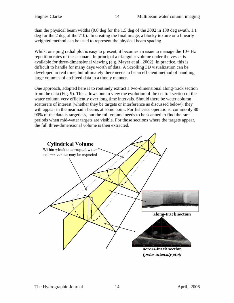
than the physical beam widths (0.8 deg for the 1.5 deg of the 3002 in 130 deg swath, 1.1 deg for the 2 deg of the 710). In creating the final image, a blocky texture or a linearly weighted method can be used to represent the physical beam spacing. Whilst one ping radial plot is easy to present, it becomes an issue to manage the 10+ Hz repetition rates of these sonars. In principal a triangular volume under the vessel is available for three-dimensional viewing (e.g. Mayer et al., 2002). In practice, this is difficult to handle for many days worth of data. A Scrolling 3D visualization can be developed in real time, but ultimately there needs to be an efficient method of handling large volumes of archived data in a timely manner. One approach, adopted here is to routinely extract a two-dimensional along-track section from the data (Fig. 9). This allows one to view the evolution of the central section of the water column very efficiently over long time intervals. Should there be water column scatterers of interest (whether they be targets or interference as discussed below), they will appear in the near nadir beams at some point. For fisheries operations, commonly 80-90% of the data is targetless, but the full volume needs to be scanned to find the rare periods when mid-water targets are visible. For those sections where the targets appear, the full three-dimensional volume is then extracted.



Fig. 9: Illustrating the method of extracting a vertical profile image, nearly equivalent to that produced by a single beam sounder. The across-track triangular sections are always available for viewing but are only

generated when water-column targets of interest are suspected. It is important to realize that the along-track section is significantly different to that of a broad beam echo sounder. Unlike a broad beam (typically 10+°) echo-sounder trace, this section reflects a fore-aft beam width of only ~ 2°. And in the across-track section you can choose to integrate a constant cross-sectional width, for example +/-10m, rather than a small angular sector. Alternately the full section within the minimum slant range can be integrated to better ensure detection of rare targets. Including data outside that semi-circle risks contaminating the water column image with bottom related variations in bottom scattering strength. Using this approach, a number of common water column echo types are illustrated and explained. Third Party Sonar Interference The performance of any mapping sonar is inherently limited by the local acoustic environment. Signal-to-noise ratios will be affected by reverberation and scattering from sources or targets other than the ones of interest. The presence of unwanted reverberation and sources is usually recognized from distinctive signatures in conventional scrolling displays of received echo intensity. Single beam echo sounders that have interference from other unsynchronized sonars are characterized by a step like periodic pattern in the echo trace map (Fig. 14, centre right).



Fig. 10: Synthetic image illustrating the geometry of direct and bottom-bounced echoes from third party sonars. In the model, due to the fact that the first arrival (the only one seen in the single beam) will occur

within a quarter of the time that the outermost beam of a 150° swath will return, the single beam is firing at a higher rate.

There are two principal methods by which a third party sonar will appear: either by direct arrival from source to receiver (or electrically through inter-cable interference), or via a bottom bounce. For a conventional single channel echo sounder which only discriminates in time, the two methods cannot easily be differentiated. For a multibeam system, where the two types of interferences are viewed in both time and angle, they look significantly different (Fig. 10). A direct path, or electrical interference will appear as a single time line in the time-angle plot (Fig. 10, top) or a single range arc in the depth-across-track plot (Fig. 10, bottom). A bottom bounce on the other hand will appear at differing times for each of the channels, looking similar, but not identical to the main bottom echo. If the two sonars have a synchronous transmit, the two echoes would be impossible to separate. But for an unsynchronized sonar, the transmit time of the interfering sonar can occur anytime (e.g. in the previous receiver cycle). The time-angle pattern is an identical arc to the real bottom echo, but bulk time-shifted. The arc tends to be less clear for two reasons: the signal is leaking through only via the relative bandwidth overlap; and the fact that the transmit is not constrained fore-aft.



As an aside, for multi-sector sonar systems, the direct arrival will not exactly correspond to the same radial distance as the three sectors fire at different times. This can be seen in the examples in Fig. 11 (top) which are derived from an EM710.

Fig. 11: Practical examples of direct arrivals in the water column (top), bottom bounced echoes (centre) and direct arrivals that intersect the seabed (bottom). EM710, HMS Endurance, EA600 12/38 kHz

interfering. When this time-shifted arc in time-angle space is converted to a depth-across-track representation, it will appear as one of a series of distinctive shapes, demonstrated in Fig 12. For the purpose of bottom detection this is less of an issue, as it should never intersect the real bottom echo. But it will show up in the water column imaging. As well as the peaked section, one will see a faint range arc at a common slant range of the first arrival (see Fig. 11 centre) corresponding to the specular single-beam echo being picked up in the multibeam receiver sidelobes. From the point of view of bottom tracking, the direct arrival is the larger issue for interference. The problem occurs when the range arc intersects the true bottom solutions (Fig. 11 bottom). Under these conditions, one will get a pair of bottom mistracks at the same radial distance on either side of the swath. As the interfering sonar will not be synchronized, those pairs of bottom tracking failures will plot as successive inboard or outboard shifting bottom-track-failure pairs.



For the purpose of water column imaging, the direct path interference occurring before the first arrival will most corrupt the water column image. For the purposes of biomass calculation (normally done through echo integration) these echoes can grossly corrupt the estimates. Vessel Engine and Propeller Noise The signal to noise ratio often is dominated by self radiated noise from the platform. The noise tends to be broad band, and strongly related to vessel speed through the water and engine revolutions. The source may be the radiated vibration of motors in the hull, or hydrodynamic noise of flow past the hull, or propeller-related turbulence. Just as with the third-party sonar interference, the noise may leak into the multibeam time series through direct transmission or through a bottom bounce. Figure 12 illustrates the appearance of bottom bounced external noise sources. As the echo is picked up from the across-track spread of receiver beam footprints, the echo will appears as a secondary parabolic arc of solutions in the time-angle projection (Fig.12 upper). This parabolic arc is offset however, depending on the time shift between the multibeam transmit and the time of the noise event. When these offset bottom echoes are reprojected from time-angle space to depth- across track space, they appear as a symmetric series of peaked sections across the image (Fig. 12 bottom). The peakedness increases as the echo appears higher in the water column.



Fig. 12: Synthetic Image modeling the mapping of unsynchronized bottom-reflected echoes. In figure 13, two polar intensity plots (Fig. 13 top) illustrate real examples of these secondary bottom bounces. As expected they are peaked. They are also prolonged compared to the seabed echo. There are two reasons for this: firstly, the arrival occurs over the full fore-aft width of the receiver beam pattern; and secondly the source function (the engine or propeller noise) need not normally be of short duration. Notably, these secondary reverberations are close to parallel to the main seabed echoes rather than intersecting like the direct arrival (Figs. 11 and 12). Unless the noise level is comparable to the bottom return, this is not normally an issue for the bottom tracking capability of the sonar. But such a reverberation may dominate over the natural mid water scattering, providing a false impression of increased density of biomass. When viewed in an along-track section (Fig. 13 lower), the water column scattering will appear to increase with depth. This is an artifact of the time–varying gain (TVG) applied to the receivers. The TVG is only appropriate for echoes whose source was at the time of the multibeam transmit. As the asynchronous echo approaches the time of transmit, it appears attenuated as it benefits from less of the TVG.



Fig. 13: Examples of ship-generated noise such as propeller or engines. Top- polar intensity plots showing the peaked secondary cross-sections due to bottom scattering of un-synchronised external noise events.

Centre- seabed backscatter strip image showing alternating mud ponds and bedrock. Bottom – Along-track water column scattering cross-section for the corresponding time of the image above. EM710 – CCGS

Matthew, Scotian Shelf. In along-track cross-section (Fig. 13 lower) one can also observe abrupt along track fluctuations in this mid-water noise. These fluctuations are directly correlated with the bottom backscatter strength. For the same time period, the seabed backscatter image is plotted (Fig.13 middle). It is clear that the abrupt drop in water column noise correlates exactly with the presence of mud-ponds. The engine noise is dominantly appearing through the bottom bounce, rather than direct arrival and therefore influenced by local bottom backscatter strength. Thus biomass estimates, which will be corrupted by bottom bounced noise, may spuriously vary due to changing bottom type. Bubble Wash Down A major limitation of any hull-mounted array is the likelyhood of bubbles being mixed into the near surface waters which may then get swept in front of the array face. The high impedance contrast between air and water results in heavy attenuation of both the outgoing energy and returned echo.



In marginal bubble wash down conditions, the result is not immediately apparent in the bottom tracking. As long as the correct range is measured, the higher background noise level is not critical. For the same echo, however, the received intensity may be attenuated by 5-10 dB. This shows up as striping in the bottom backscatter strength (Fig. 14), degrading the backscatter mosaic.

Fig. 14: Top – showing presence and absence (a few pings later) of a bubble wash down layer.. Centre- vertical section of near nadir water-column scattering showing intermittent near-surface scattering events

corresponding to bubble wash down. For the second half of the time series, the ship’s 12/38 kHz echo sounder is turned on illustrating the appearance of unsynchronized sonars (Figs. 10 and 11). Bottom –

equivalent sidescan strip image corresponding to the water column image, showing how the high bubble wash-down tends to correlate with across-track striping in the sidescan. EM710, HMS Endurance.

As the bubble wash-down increases, the bottom tracking will get noisier and ultimately mistracks will result. The obvious solution to this problem is to avoid bubble wash down at all, either by retrimming the vessel, adjusting the vessel speed or azimuth, mounting the array on a gondola or simply not surveying until sea state conditions improve. The onset of bubble wash-down is a critical issue that has huge financial consequences for the cost of survey. To be able to monitor the bubble sweep mechanism would be highly advantageous. Such an approach is now possible using the early part of the multibeam water column data. From the point of view of the water column data, bubble wash down primarily masks echoes (note lower water column echo intensity in Figure 14



centre). For the very first part of the time series, however, it should be possible to see the scattering from the bubble later. Figure 14 (top) illustrates the appearance of bubble wash-down in the polar- intensity plots. Note that the apparent depth of the layer may be larger than the real depth due to internal multiple bounces from within the bubble layer. When viewed in a vertical along-track cross-section (Fig. 14 centre) the bubble wash down appears as periodic, near-surface bright spots. These bright spots tend to be correlated with pitching and show up as attenuated pings (lower backscatter) in the corresponding seabed backscatter strip (Fig. 14 lower). One has to realize that, whilst the received time series is produced from times immediately after transmit to the maximum two-way travel time, the data in the bubble wash down region is always in the near field. Without focusing this would be an issue. The EM3002 and EM710, however, are focused on receive. The EM710 also focuses on transmit (something that is not practical for a single sector system as the required focal length varies so greatly). Bottom Tracking Issues Ideally, with sufficient sidelobe suppression, the intended section of the seafloor within the main lobe of the transmit-receive product should be tracked. Under conditions of benign seafloor geometry and locally invariant distribution of seabed bottom backscatter strength, side lobe suppression is normally sufficient to guarantee a correct bottom lock. However under complex seafloor geometries, often a combination of optimal grazing angle (providing near specular echoes) and extreme variations in bottom backscatter strength (providing anomalously strong echoes outside the mainlobe footprint) can conspire to produce a bottom mistrack.



Fig. 15: Example showing bottom mis-tracking under extreme geometry (drowned terrestrial canyon). Without recourse to the full intensity time series, the relationship of the mis-tracks to the peg-leg multiple

could not be established. EM3002, Wahweap Canyon, Lake Powell AZ. A particularly extreme example is presented of imaging a drowned canyon system (Fig. 15). In this image, the true shape of the canyon walls can be clearly seen in the polar intensity plot. But as the canyon walls are very smooth and normally not specular, other echoes can dominate. These can include peg-leg multiples that are actually logged by the receiver main lobe, but whose ensonification came about by a specular bounce off the other sidewall of the canyon (the false bottom tracking has locked onto the peg-leg echo on the right side of the image in figure 15). Alternately, sidelobe echoes from planar specular facets such as the flat canyon floor below, or even inward facing rock surfaces on the flanks of the canyon (Fig. 15), can produce echoes stronger than the true terrain in the beam mainlobe. Such a geometry can exist, even with more benign seafloors. In the synthetic example in Figure 4, one sees that inward facing slopes which are near specular can produce potential false solutions up arc and down arc of the true seafloor. A similar phenomena is commonly noted in boulder strewn terrains (modeled in Figure 5) where the specular inward facing surface of the boulder produces an arc of high intensity at that slant range centred on the face of the boulder. False tracking often occurs along this arc, providing



false deeper solutions inboard, and a misleadingly false minimum depth over the top of the boulder. Wreck Delineation One of the prime concerns with multibeam topographic resolution is the adequate delineation of the minimum clearance over man-made objects such as wrecks. At this time, several agencies still require wreck sweeping to ensure physical evidence for minimum clearance. This normally involves wire or bar sweeping that is extremely expensive in ship time, but unambiguous. Two examples are presented of wrecks with proud mast-like features using an EM3002 (Fig. 6)) and an EM710 (Figs. 16 and 17). In both cases, small green dots are superimposed showing the bottom track solutions. In both cases, the bottom tracks never lock onto the shallowest echoes. The reasons for these are speculated to be two-fold:

- firstly the echoes identified are neither the strongest, nor the only significant ones at that beam azimuth.

- secondly the bottom tracking involves using gates, which have not been able to respond to the abrupt appearance (and subsequent disappearance ) of the shallower targets.

In both cases, by using the water column image and hindsight (knowing that a wreck is present) one is able to infer that a shallower target really exists. Care has to be taken in interpretation, as there are many other reasons why false mid-water targets may appear. This is especially true in the case of a wreck where there are many corner scatterers, and planar flat surfaces (e.g. decks). A confident interpretation requires a full understanding of likely sidelobe echo geometry and its resulting appearance in the polar intensity plots. For example, in Figure 6 (centre), the echo from the deck surface, picked up in sidelobes produces a range arc of moderate intensity backscatter, apparently in the water-column on either side of the wreck, which extends right out to the edges of the swath (as the EM3002 is a single sector transmit system). It would be near-impossible to examine whether fish are schooling in this region. And in Figure 16, the deck surface again produces a misleading arc of moderate intensity scattering in the water column. Only in this case (a multi-sector EM710), the arc terminates at the sector boundary as the outer sector transmit beam pattern does not ensonify the deck surface. In Figure 6 (centre left image), the clear signature of a raised feature (probably a partially collapsed mast) is seen, but does not mask the echo from the deck below. There are probably three reasons that the mast does not fully occlude the beam:

• firstly the subtended solid angle of the beam, at the slant range of the mast, is larger than the mast cross-section and thus significant energy makes it past the mast;



• secondly the deck is also illuminated by the transmit sidelobes both ahead and behind the mast;

• and thirdly the deck echo, being planar is likely to produce a far stronger echo. In this case it is clear that the trained hydrographer can infer the true shallowest point on a wreck far more confidently from the polar intensity plot than from the real-time automated bottom detection algorithm. The algorithm could be adjusted to pick up the echo in question, but by doing so, the algorithm would become unreasonably sensitive to mid-water anomalies elsewhere providing an unmanageable level of false tracking in otherwise benign seafloors. For example, if a threshold exceeding criteria were used instead of a peak echo strength, the system would likely lock onto sidelobe echoes from out-of-beam specular echoes.

Fig. 16: Intensity image showing clear target proud of the wreck deck. The intensity of the target echo, is

however weaker than the echo from the deck surface beyond (and hence the bottom track solution does not track the real feature). This implies that the target does not fully occlude the deck, i.e. that the object

(probably a mast) is smaller than the projected cross-section of the beam. Whilst polar intensity plots provide an second opportunity to detect mast-like targets, physical limitations in the geometry and angular resolution will restrict the method. In Figure 17, for example, the same wreck is ensonified at much lower grazing angles. In this case the broader beamwidths and the presence of sidelobe contributions from the inboard seafloor make it harder to subjectively pick out the mast top. It would be prudent to have a strategy of undertaking a dedicated pass directly over wreck targets. Even then, this would be cheaper than a wire sweep. It should be noted that the examples used here



involve 1.5° to 2°+ beams. With the availability of narrower beamed systems, the likelyhood of the mast-like target completely occluding the wreck behind would be improved. An alternate strategy of re-shading the beams to reduce sidelobes could also be beneficial.

Fig. 17: Polar intensity image over exactly the same cross section of the wreck as figure 16. In this case,

the wreck has been shifted out into the low grazing angle region. The ship’s deck and the proud target now lie at or beyond the slant range of the first seafloor arrival. Also the steered beams are now almost twice as

wide. The proud target (probably a gantry or mast stub) is still clearly present (in hindsight). By combining the polar intensity plot from multiple passes, small, potentially weak, but repeatable targets

can be identified with confidence. Oceanographic Imaging It has long been recognized that patterns seen in water column scattering profiles are often a good indicator of the distribution of watermasses (Munk and Garrett 1973, Proni and Appel, 1975). Strong variations in salinity (haloclines) and temperature (thermoclines) show up particularly well. The acoustic signature of watermasses (or more specifically their boundaries) is often defined by variations in density and sound speed (Thorpe and Brubaker, 1983), zones of turbulence (Oakey and Cochrane, 1998) and the presence of zooplankton species (Stanton et al., 1994, 1998). Spatial variability in the location and intensity of the thermocline is of direct interest to the hydrographic surveyor (Hughes Clarke and Parrot, 2001). In the open ocean, sound speed variability is primarily controlled by temperature. Inshore, in estuarine



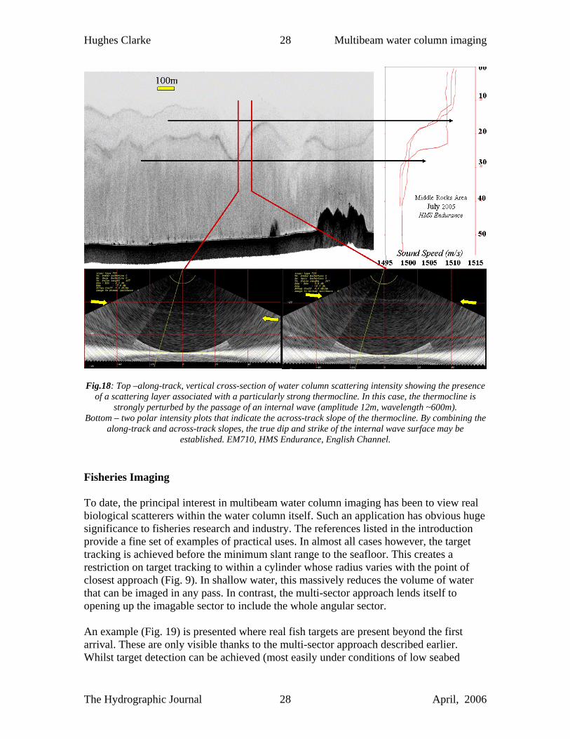
environments the halocline is of more interest (Hughes Clarke and Haigh, 2005). The presence, intensity and depth of the principal velocline will strongly control the refracted ray path. Usually, the depth of the principal thermocline varies slowly in an area of interest. Sound speed profiles at time intervals of several hours should suffice to capture the temporal and spatial variability of its location. Under strongly stratified summer conditions however, the density contrasts can be extreme and internal tides can develop strong internal wave fields on the interface. Such internal waves can have amplitudes of several 10’s of metres over wavelengths less than a kilometre. Such short wavelength variability is hard to capture, even with the latest underway mechanical profiling equipment (Furlong et al., 2000, de Silva et al., 2000, Hughes Clarke et al. 2000). Acoustic imaging, whilst strictly only a qualitative indicator, updates as often as the sonar fires, providing a means of monitoring the likely location of thermocline over shorter spatial distances. The example below (fig. 18) illustrates the imaging of a particularly strong thermocline in the English Channel during the summer. The vertical along track profile (nearly equivalent to the output of a single beam echosounder) clearly recognizes a primary strong scattering layer that corresponds closely to the depth of the main thermocline (identified from 6 hourly CTD casts). The depth and sharpness of the scattering layer were found to vary widely over the survey area. From an oceanographic point of view, the propagation direction of the internal wave is of great interest. A single two-dimensional cross-section provides only a projected image of the wave. Two or more offset profiles are required to establish a strike. And even then, as the wave will have propagated in the time it takes for the second profile to be acquired, the true orientation is hard to establish. Using the across track image within the polar intensity plot (Fig. 18 lower), one can establish if there is an across-track slope to the scattering layer. This allows one to calculate the strike and dip of the internal wave surface, thereby providing an instantaneous propagation direction. That the layer is visible at oblique incidence indicates that the source of the returned acoustic energy is a scattering phenomenon (most likely related to turbulence or biomass) rather than coherent reflection related to the impedance contrast at the interface.



Fig.18: Top –along-track, vertical cross-section of water column scattering intensity showing the presence

of a scattering layer associated with a particularly strong thermocline. In this case, the thermocline is strongly perturbed by the passage of an internal wave (amplitude 12m, wavelength ~600m).

Bottom – two polar intensity plots that indicate the across-track slope of the thermocline. By combining the along-track and across-track slopes, the true dip and strike of the internal wave surface may be

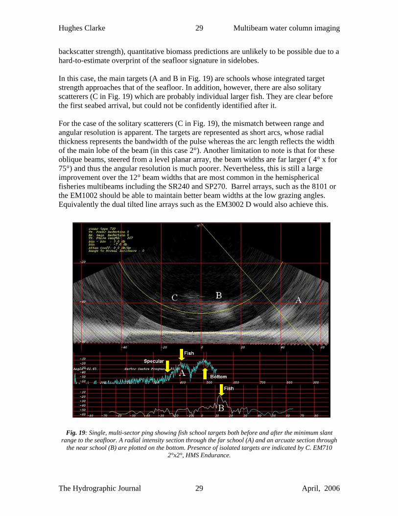
established. EM710, HMS Endurance, English Channel. Fisheries Imaging To date, the principal interest in multibeam water column imaging has been to view real biological scatterers within the water column itself. Such an application has obvious huge significance to fisheries research and industry. The references listed in the introduction provide a fine set of examples of practical uses. In almost all cases however, the target tracking is achieved before the minimum slant range to the seafloor. This creates a restriction on target tracking to within a cylinder whose radius varies with the point of closest approach (Fig. 9). In shallow water, this massively reduces the volume of water that can be imaged in any pass. In contrast, the multi-sector approach lends itself to opening up the imagable sector to include the whole angular sector. An example (Fig. 19) is presented where real fish targets are present beyond the first arrival. These are only visible thanks to the multi-sector approach described earlier. Whilst target detection can be achieved (most easily under conditions of low seabed



backscatter strength), quantitative biomass predictions are unlikely to be possible due to a hard-to-estimate overprint of the seafloor signature in sidelobes. In this case, the main targets (A and B in Fig. 19) are schools whose integrated target strength approaches that of the seafloor. In addition, however, there are also solitary scatterers (C in Fig. 19) which are probably individual larger fish. They are clear before the first seabed arrival, but could not be confidently identified after it. For the case of the solitary scatterers (C in Fig. 19), the mismatch between range and angular resolution is apparent. The targets are represented as short arcs, whose radial thickness represents the bandwidth of the pulse whereas the arc length reflects the width of the main lobe of the beam (in this case 2°). Another limitation to note is that for these oblique beams, steered from a level planar array, the beam widths are far larger ( 4° x for 75°) and thus the angular resolution is much poorer. Nevertheless, this is still a large improvement over the 12° beam widths that are most common in the hemispherical fisheries multibeams including the SR240 and SP270. Barrel arrays, such as the 8101 or the EM1002 should be able to maintain better beam widths at the low grazing angles. Equivalently the dual tilted line arrays such as the EM3002 D would also achieve this.

Fig. 19: Single, multi-sector ping showing fish school targets both before and after the minimum slant

range to the seafloor. A radial intensity section through the far school (A) and an arcuate section through the near school (B) are plotted on the bottom. Presence of isolated targets are indicated by C. EM710

2°x2°, HMS Endurance.



Conclusions The recent availability of water column imaging from hydrographic-grade multibeam echo-sounders provides the hydrographic surveyor with a new suite of tools to better implement quality control on survey data. The principal advantages include:

• Better identification and recognition of stray noise sources including: o 3rd party interfering sonars. o Ship generated noise such as machinery, flow or propeller. o Bubble wash down

• Improved confidence in bottom tracking in abrupt geometries. • Greater ability to estimate the minimum clearance over wrecks (possibly to the

point that wire sweeping would not be necessary) • The ability to image thermocline structure and thus predict variability in the sound

speed field. The same data also provide a new market for hydrographic data by imaging the spatial distribution of biological scatterers in the water column. Whilst still meeting the prime needs of bathymetric survey, a whole new market of clients is opening up. Acknowledgements This work has greatly benefited from the open availability of water column data from the Canadian Hydrographic Service (Mike Lamplugh) and the Royal Navy (Commander Bungy Williams). The officers and crew of CCGS Matthew and HMS Endurance ably supported the data collection programs. EM3002 data was obtained using hardware loaned by Kongsberg Seattle (Lake Powell) and from CSL Heron. The Powell data were acquired by the author and Jonathan Beaudoin, and the Heron data were acquired by Steve Brucker and Jason Bartlett. Support for salaries and hardware used as part of this research has come from the sponsors of the Chair in Ocean Mapping at UNB. These currently include the Canadian Hydrographic Service, Kongsberg Maritime, the US Geological Survey, the Centre for Coastal and Ocean Mapping, Fugro Pelagos, the Royal Navy and the UK Hydrographic Office, Rijkswaterstaat and the Route Survey Office of the Canadian Navy. References Axelsen, B.E., T. Anker-Nilssen, P. Fossum, C. Kvamme, and L. Nøttestad, 2001, Pretty patterns but a simple strategy: predator-prey interactions between juvenile herring and Atlantic puffins observed with multibeam sonar: Can. J. Zool. 79, 1586–1596



Benoit-Bird K., and W. Au, 2003, Hawaiian spinner dolphins aggregate midwater food resources through cooperative foraging: J. Acoust. Soc. Am. 114, 2300 Cochrane, N.A., Y. Li, and G. D. Melvin, 2003, Quantification of a multibeam sonar for fisheries assessment applications: J. Acoust. Soc. Am. 114, 745–758 DaSilva, J.L., Bridges, W., Grady,J., Aucoin, B., Pastor, C. and Reed, 2000, Multibeam hydrography: Improving error budget estimates and efficiency: Canadian Hydrographic Conference 2000, CDROM. Foote, K.G., D. Chu, T. R. Hammar K. C. Baldwin, L. A. Mayer L. C. Hufnagle, Jr.and J. M. Jech, 2005, Protocols for calibrating multibeam sonar: J. Acoust. Soc. Am., Vol. 117, No. 4, Pt. 1, p. 2013–2027 Furlong, A., Hazen,D., and Bugden, G., 2000, Near vertical water column profiling using a Moving Vessel Profiler (MVP): Oceanology 2000, Conference Proceeding, CDROM, paper # 51. Gallaudet, T.C., and C. P. de Moustier, 2003, High-frequency volume and boundary acoustic backscatter fluctuations in shallow water,’’ J. Acoust. Soc. Am. 114, 707–725. Gerlotto, F., P. Fre´on, M. Soria, P. H. Cottais, and L. Ronzier, 1994, Exhaustive observations of the 3D schools structure using multibeam sidescan sonar: potential use for school classification, biomass estimation, and behavior studies: Council Meeting of the Int. Council Explor. Sea 1994/B:26 Gerlotto, F., M. Soria, and P. Fre´on, 1999, From two dimensions to three: the use of multibeam sonar for a new approach in fisheries acoustics: Can. J. Fish. Aquat. Sci. 56, 6–12 Hafsteinsson, M.T., and O. A. Misund, 1995, Recording the migration behavior of fish schools by multibeam sonar during conventional acoustic surveys: ICES J. Mar. Sci. 52, 915–924 Hammerstad, E., 1997, Multibeam echo sounder for EEZ mapping. Proceedings of OCEANS '97, 2(787). Hughes Clarke, J.E., Lamplugh, M. and Kammerer, E., 2000, Integration of near-continuous sound speed profile information: Canadian Hydrographic conference 2000, Proceedings CDROM. Hughes Clarke, J.E. and Parrot, R., 2001, Integration of dense, time-varying water column information with high-resolution swath bathymetric data : United States Hydrographic Conference Proceedings, CDROM. 9pp.



Hughes Clarke, J.E. and Haigh, S.P. (2005), Observations and interpretation of mixing and exchange over a sill at the mouth of the Saint John river estuary. Proceedings of the 2nd CSCE Specialty Conference on Coastal, Estuary and Offshore Engineering, Toronto, Canada, June 2-4. Jones, C.D., 2003, Water-column measurements of hydrothermal vent flow and particulate concentration using multibeam sonar: J. Acoust. Soc. Am. 114, 2300–2301 Kongsberg Simrad A/S 1998, EM1002 Multibeam Sonar Operators Manual, Horten, Norway. Kongsberg Simrad Maritime, 2004, EM3002 Multibeam Sonar Operators Manual, Horten Norway Kongsberg Maritime, 2005, EM710 Multibeam Sonar Operators Manual, Horten Norway. Kraeutner, P. H., & J. S. Bird, 1995, Seafloor scatter induced angle of arrival errors in swath bathymetry sidescan sonar. Proceedings IEEE OCEANS '95: MTS/IEEE, New York, NY, 2: 975-980. Mayer, L.A., Y. Li, and G. Melvin, 2002, 3-D visualization for pelagic fisheries assessment and research, ICES, v.59, no.1, p.216-225 Misund, O.A., and A. Aglen, 1992, Swimming behavior of fish schools in the North Sea during acoustic surveying and pelagic trawl sampling,’’ ICES J. Mar. Sci. 49, 325–334 Misund, O.A., 1993, Dynamics of moving masses: variability in packing density, shape, and size among herring, sprat and saithe schools,’’ ICES J. Mar. Sci. 50, 145–160. Munk, W.H. and J.C.R. Garrett, 1973. "Internal wave breaking and microstructure (The chicken and the egg)." Boundary Layer Meteorol. 4, 37-45. Nøttestad, L., and B. E. Axelsen, 1999, Herring schooling manoeuvres in response to killer whale attacks,’’ Can. J. Zool. 77, 1540–1546 Oakey, N.S. and Cochrane, N.A., 1998, Turbulent Mixing in Solitons: IOS/WHOI/ONR Internal Solitary Wave Workshop Papers. 6th Edition, WHOI Technical Report number WHOI-99-07. http://www.whoi.edu/science/AOPE/people/tduda/isww/text/index.html Poehner, F., & E. Hammerstad, 1991, Combining bathymetric mapping, seabed imaging. Sea Technology 32(6): 17-25. Proni, J.R. and J.R. Apel, 1975. "On the use of high-frequency acoustics for the study of internal waves and microstructure," J. Geophys. Res. 80, 1147-1151.



Soria, M., P. Fre´on, and F. Gerlotto, 1996, Analysis of vessel influence on spatial behaviour of fish schools using a multi-beam sonar and consequences for biomass estimates by echo-sounder: ICES J. Mar. Sci. 53, 453–458 Stanton, T.K., P.H. Wiebe, D. Chu, and L. Goodman, 1994. "Acoustic characterization and discrimination of marine zooplankton and turbulence," ICES J. Mar. Sci., 51, 469-479. Stanton, T.K., Warren, J.D., Wiebe, P.H., Benfield M.C. and Greene, C.H., 1998, Contributions of the Turbulence Field and Zooplankton to Acoustic Backscattering by an Internal Wave: IOS/WHOI/ONR Internal Solitary Wave Workshop Papers. 6th Edition, WHOI Technical Report number WHOI-99-07. http://www.whoi.edu/science/AOPE/people/tduda/isww/text/index.html Thorpe, S.A. and J.M. Brubaker, 1983: Observations of Sound Reflection by Temperature Microstructure: Limnology and Oceanography, 28, 601-613. Weber, T., D. Bradley, R. L. Culver, and A. Lyons, 2003, Inferring the vertical turbulent diffusion coefficient from backscatter measurements with a multibeam sonar: J. Acoust. Soc. Am. 114, 2300


applications of multibeam water column imaging for ... of multibeam water column imaging for...

Documents