applications of the probabilistic method to random …moore/vishalthesis.pdfapplications of the...
TRANSCRIPT
Applications of the Probabilistic Method toRandom Graphs
by
Vishal Sanwalani
B.A., Finance, Economics, and Biology, Washington University, 1997
DISSERTATION
Submitted in Partial Fulfillment of the
Requirements for the Degree of
Doctor of PhilosophyComputer Science
The University of New Mexico
Albuquerque, New Mexico
July, 2005

c©2005, Vishal Sanwalani
iii

Acknowledgments
I would like to thank my advisor, Professor Cristopher Moore, for giving me the freedom to learn.I would like to thank Professor Jared Saia for exposing me to new areas in Computer Science.I would like to thank my committee members Professor Shuang Luan and Professor VladimirKoltchinskii for their helpful comments and suggestions. I would like to thank Professor JosepDiaz for all the valuable advice and help he has given me. Finally, I would like to thank all mycoauthors, much of the work in this thesis was done jointly with their help.
iv
Applications of the Probabilistic Method toRandom Graphs
by
Vishal Sanwalani
ABSTRACT OF DISSERTATION
Submitted in Partial Fulfillment of the
Requirements for the Degree of
Doctor of PhilosophyComputer Science
The University of New Mexico
Albuquerque, New Mexico
July, 2005

Applications of the Probabilistic Method toRandom Graphs
by
Vishal Sanwalani
B.A., Finance, Economics, and Biology, Washington University, 1997Ph.D., Computer Science, University of New Mexico, 2005
Abstract
We discuss three problems. Although the problems themselves are distinct, two basic themes
underly each of them. First, each problem is either directly, or can be viewed as a random
graph problem. Second, all the problems can be solved by using elementary techniques from
the probabilistic method. We first discuss the Leader Election problem. In the leader election
problem, there are n processors, βn of which are bad (or corrupt), and (1 − β)n of which are
good, for some fixed β. For β < 1/3, we present an algorithm which elects a leader from the set
of all processors such that, with constant probability, this leader is good, and a 1− o(1) fraction
of the good processors know the election result. Further the algorithm only requires each good
processor to send and process a number of bits which is polylogarithmic in n.
Next we discuss the chromatic number of a random scaled sector graph. In the random scaled
sector graph model, vertices are placed uniformly at random into the [0, 1]2 unit square. Each
vertex i is assigned a uniformly at random sector Si, of central angle αi, in a circle of radius ri
(with vertex i as the origin). An arc is present from vertex i to any vertex j, if j falls in Si. We
study the value of the chromatic number χ(Gn), for random scaled sector graphs with n vertices,
vi

where each vertex spans a sector of α degrees with radius rn =√
ln nn
. We prove that for values
α < π, as n → ∞ w.h.p., χ(Gn) is Θ( ln nln ln n
). For α > π w.h.p. (with high probability), χ(Gn)
is Θ(ln n).
Finally, we discuss the probability a sparse random graph or hypergraph is connected. While
it is exponentially unlikely that a sparse random graph or hypergraph is connected, with probabil-
ity 1−o(1) such a graph has a “giant component” that, given its numbers of edges and vertices, is
a uniformly distributed connected graph. This simple observation allows us to estimate the num-
ber of connected graphs, and more generally the number of connected d-uniform hypergraphs,
on n vertices with ((d− 1)−1 + Ω(1))n ≤ m = o(n ln n) edges.
vii

Contents
List of Figures xii
1 Scalable Leader Election 1
1.1 Acknowledgements . . . . . . . . . . . . . . . . . . . . . . . . . . . . . . . . . 1
1.2 Introduction . . . . . . . . . . . . . . . . . . . . . . . . . . . . . . . . . . . . . 1
1.2.1 Problem Statement . . . . . . . . . . . . . . . . . . . . . . . . . . . . . 2
1.2.2 Our Results . . . . . . . . . . . . . . . . . . . . . . . . . . . . . . . . . 3
1.2.3 Related Work . . . . . . . . . . . . . . . . . . . . . . . . . . . . . . . . 4
1.2.4 Roadmap . . . . . . . . . . . . . . . . . . . . . . . . . . . . . . . . . . 5
1.3 Preliminaries . . . . . . . . . . . . . . . . . . . . . . . . . . . . . . . . . . . . 5
1.4 The Layered Network . . . . . . . . . . . . . . . . . . . . . . . . . . . . . . . . 9
1.5 Communication and validation . . . . . . . . . . . . . . . . . . . . . . . . . . . 10
1.5.1 Monitoring sets . . . . . . . . . . . . . . . . . . . . . . . . . . . . . . . 10
1.5.2 Validation between monitoring sets . . . . . . . . . . . . . . . . . . . . 11
viii

Contents
1.5.3 Downward communication tree . . . . . . . . . . . . . . . . . . . . . . 13
1.5.4 The Communications Protocol . . . . . . . . . . . . . . . . . . . . . . . 13
1.6 The Leader Election Algorithm . . . . . . . . . . . . . . . . . . . . . . . . . . . 14
1.7 Proof of Theorem 1 . . . . . . . . . . . . . . . . . . . . . . . . . . . . . . . . . 15
2 The chromatic number of random scaled sector graphs 21
2.1 Acknowledgements . . . . . . . . . . . . . . . . . . . . . . . . . . . . . . . . . 21
2.2 Introduction . . . . . . . . . . . . . . . . . . . . . . . . . . . . . . . . . . . . . 21
2.3 Results . . . . . . . . . . . . . . . . . . . . . . . . . . . . . . . . . . . . . . . . 23
2.4 Basic constructions and lemmas . . . . . . . . . . . . . . . . . . . . . . . . . . 24
2.5 Proof of Theorem 1 . . . . . . . . . . . . . . . . . . . . . . . . . . . . . . . . . 27
2.5.1 α < π − ε . . . . . . . . . . . . . . . . . . . . . . . . . . . . . . . . . . 27
2.5.2 α > π + ε . . . . . . . . . . . . . . . . . . . . . . . . . . . . . . . . . 27
2.5.3 α = 2π . . . . . . . . . . . . . . . . . . . . . . . . . . . . . . . . . . . 32
2.6 Proof of Theorem 2 . . . . . . . . . . . . . . . . . . . . . . . . . . . . . . . . . 32
2.6.1 α > π + ε . . . . . . . . . . . . . . . . . . . . . . . . . . . . . . . . . . 32
2.6.2 ε < α < π − ε . . . . . . . . . . . . . . . . . . . . . . . . . . . . . . . 33
2.7 Proof of Theorem 3 . . . . . . . . . . . . . . . . . . . . . . . . . . . . . . . . . 36
2.7.1 α > π + ε . . . . . . . . . . . . . . . . . . . . . . . . . . . . . . . . . 36
2.7.2 α < π − ε . . . . . . . . . . . . . . . . . . . . . . . . . . . . . . . . . 37
2.8 Conclusions and open problems . . . . . . . . . . . . . . . . . . . . . . . . . . 37
ix

Contents
3 Counting Connected Graphs and Hypergraphs via the Probabilistic Method 42
3.1 Acknowledgements . . . . . . . . . . . . . . . . . . . . . . . . . . . . . . . . . 42
3.2 Introduction and Results . . . . . . . . . . . . . . . . . . . . . . . . . . . . . . 42
3.2.1 Results . . . . . . . . . . . . . . . . . . . . . . . . . . . . . . . . . . . 43
3.2.2 Techniques and Overview . . . . . . . . . . . . . . . . . . . . . . . . . 47
3.2.3 Related Work . . . . . . . . . . . . . . . . . . . . . . . . . . . . . . . . 49
3.3 Preliminaries . . . . . . . . . . . . . . . . . . . . . . . . . . . . . . . . . . . . 51
3.4 The Number of Connected Hypergraphs . . . . . . . . . . . . . . . . . . . . . . 53
3.4.1 Outline . . . . . . . . . . . . . . . . . . . . . . . . . . . . . . . . . . . 53
3.4.2 Proof of Lemma 2 . . . . . . . . . . . . . . . . . . . . . . . . . . . . . 58
3.4.3 Proof of Lemma 3 . . . . . . . . . . . . . . . . . . . . . . . . . . . . . 58
3.4.4 Proof of Lemma 4 . . . . . . . . . . . . . . . . . . . . . . . . . . . . . 60
3.5 The Probability of Getting a Giant Component of a Given Order and Size . . . . 61
3.5.1 Outline . . . . . . . . . . . . . . . . . . . . . . . . . . . . . . . . . . . 61
3.5.2 Proof of Lemma 7 . . . . . . . . . . . . . . . . . . . . . . . . . . . . . 66
3.5.3 Proof of Lemma 8 . . . . . . . . . . . . . . . . . . . . . . . . . . . . . 67
3.5.4 Proof of Lemma 9 . . . . . . . . . . . . . . . . . . . . . . . . . . . . . 68
3.6 The Expected Number of Edges Given that Hd(n, p) is Connected . . . . . . . . 70
3.7 Branching Processes and The Giant Component of Hd(n, p) . . . . . . . . . . . 71
3.7.1 Preliminaries on Branching Processes . . . . . . . . . . . . . . . . . . . 72
x

Contents
3.7.2 Exploring the Components of Hd(n, p) . . . . . . . . . . . . . . . . . . 76
3.7.3 Large Deviations of N (Hd(n, p)) and the Number of Isolated Vertices . . 83
3.7.4 The Variance of N (Hd(n, p)) . . . . . . . . . . . . . . . . . . . . . . . 85
3.7.5 The Variance of the Number of Edges Outside the Giant . . . . . . . . . 88
3.7.6 Proof of Lemma 14 . . . . . . . . . . . . . . . . . . . . . . . . . . . . . 93
References 95
xi
List of Figures
2.1 The sector of a sensor i and the communication between motes . . . . . . . . . 23
2.2 Angle partition for α > π + ε (a) classes B (b) directions associated to a class Bj 25
2.3 The basic dissections of [0, 1]2 (a) S (b) horizontal subdivision (c) vertical sub-
division . . . . . . . . . . . . . . . . . . . . . . . . . . . . . . . . . . . . . . . 26
2.4 Proof of lower bound . . . . . . . . . . . . . . . . . . . . . . . . . . . . . . . 39
2.5 Partition of S by strips . . . . . . . . . . . . . . . . . . . . . . . . . . . . . . . 40
2.6 Sector Si and complementary sector S∗i . . . . . . . . . . . . . . . . . . . . . . 40
2.7 Figure for the proof of 5.2 . . . . . . . . . . . . . . . . . . . . . . . . . . . . . 41
2.8 Partition of S in the prove 5.2 . . . . . . . . . . . . . . . . . . . . . . . . . . . 41
xii

Chapter 1
Scalable Leader Election
1.1 Acknowledgements
I would like to thank Valerie King, Jared Saia, and Erik Vee. The work in this chapter was done
jointly with them.
1.2 Introduction
Leader election is a fundamental problem in distributed computing. We consider this problem in
the setting where there are n processors, βn of which are bad (or corrupt), and (1−β)n of which
are good, for some fixed β. We assume that an omniscient and computationally unbounded
adversary picks which processors will be bad before the algorithm begins and this adversary
controls the actions of all bad processors so as to maximize the chance of getting a bad processor
elected. Our goal is to design an algorithm which ensures a good processor will be elected
with constant probability, no matter which set of βn processors are bad. This problem was first
formally described and addressed by Ben-Or and Linial [4, 5] about twenty years ago. Since then,
1

Chapter 1. Scalable Leader Election
many papers have been published giving leader election algorithms that successively improve on
the number of rounds required and on the fraction β of bad processors that can be tolerated [18,
1, 2, 7, 6, 9, 15, 17, 12] (see also surveys by Ben-Or, Linial and Saks [3] and Linial [14]).
In this chapter, we describe a leader election algorithm which is scalable, in the sense it
requires each good processor to send and process a number of bits which is polylogarithmic in
n.
1.2.1 Problem Statement
The standard model for communication in the leader election problem is the full information
model1 [4, 5]. In this model, all communication occurs by broadcast and is known publicly
to all processors. Every processor has a unique name known to everyone and the name of the
sender of any message is explicitly known by all processors. Communication occurs in rounds.
In each round, every processor may communicate with all other processors. The bad processors
are assumed to have received the messages of all the good processors before they broadcast their
own messages. The processors are synchronized between rounds so that all messages in round i
are assumed to be received before any messages in round i + 1 are sent out. Since the adversary
is computationally unbounded, this disallows the use of cryptographic assumptions.
The full information model rules out from the very start any possibility of designing an al-
gorithm where each processor sends a sublinear number of bits. In particular, since all commu-
nication is by broadcast, every time a node communicates in this model, it sends out Ω(n) bits.
To get around this problem, we use the point-to-point full information model. In this model, all
communication occurs between a single sender and a single receiver. The bad processors see all
messages but the good processors only see messages that are sent directly to them. Everything
else is the same as in the full information model. In particular, each processor has a unique name
which is known explicitly to anyone to whom it sends messages. Further, communication occurs
1This is sometimes also referred to as the perfect information model.
2

Chapter 1. Scalable Leader Election
in rounds and the bad processors see all messages before they need to send their own. This new
model is strictly harder than the standard full information model in the following sense. In the
standard model, in a single round, a bad processor is forced to send the same message to all
processors (since communication is by broadcast). However, in the new model, a bad processor
can send different messages to different processors.
Our goal is to minimize the number of bits sent and processed by every good processor. We
assume that a processor can choose to ignore (not process), without cost, messages received from
any other processor during any round of the algorithm.
1.2.2 Our Results
We conjecture, if a constant fraction of the processors are bad, then any algorithm which insures
with positive probability a good leader is elected and all good processors know the leader, will
require each processor to send and process Ω(n) bits. Thus, we relax the requirement that all
good processors know the leader at the end of the protocol to the requirement that a 1 − o(1)
fraction of good processors know the leader. Our main result is stated as Theorem 1 below.
To the best of our knowledge, this is the first result for the leader election problem where each
processor is required to send and process a sub-linear number of bits.
Theorem 1 Assume there are n processors and strictly less than a 1/3 fraction of these proces-
sors are bad. Then there exists an algorithm that elects, with constant probability, a leader from
the set of good processors and has the following properties.
• Exactly one good processor considers itself the leader.
• A 1− o(1) fraction of the good processors know this leader.
• Every good processor sends and processes only a polylogarithmic (in n) number of bits.
• The number of rounds required is polylogarithmic in n.
3
Chapter 1. Scalable Leader Election
1.2.3 Related Work
The first results for leader election in the full information model are due to Ben-Or and Linial [4,
5]. They give a one round protocol which is robust to up to a 1/ ln n fraction of bad processors.
Kahn, Kalai and Linial [13] show that if each good processor is restricted to providing one
random bit, then 1/ ln n is the largest fraction of bad processors that can be tolerated for any one
round protocol. Saks [18] and Ajtai and Linial [1] designed “baton-passing” protocols which
are robust to a 1/ ln n fraction of bad processors. Saks [18] also showed that no protocol can
be robust against dn/2e bad processors. Alon and Naor [2] designed a modified baton-passing
protocol which they showed to be robust to βn bad processors for any β < 1/3. Further analysis
of Alon and Naor’s protocol by Boppana and Narayanan [7, 6] showed that the protocol was
robust to βn bad processors for all β < 1/2− ε and positive ε.
The protocol due to Alon and Naor has optimal resilience but requires a linear number of
rounds. Several subsequent papers focused on reducing the number of rounds [9, 15, 19, 17].
Russell and Zuckerman [17] designed a protocol which is resilient against (1 − ε)n/2 bad pro-
cessors and takes only ln∗ n rounds. Russell, Saks and Zuckerman [16] further showed that
Ω(ln∗ n) rounds are necessary if in every round the good processors each send one unbiased ran-
dom bit. Finally, Feige [12] designed a much simpler protocol which requires O(ln∗ n) rounds
and in the situation where there are (1 + δ)n/2 good processors, elects a good processor with
probability Ω(δ1.65). All previous protocols had success probability which was exponentially
small in δ. 2 All of these algorithms require each processor to send and process Ω(n) bits, yet
it is difficult to directly compare our result with previous algorithms. First, the previous algo-
rithms assumed messages were sent via broadcast, hence the focus was on reducing the number
of rounds required. Second, we have relaxed the assumption every good processor knows the
leader (if messages are broadcast this assumption is trivially satisfied).
2The success probability was still constant provided that δ was constant.
4

Chapter 1. Scalable Leader Election
1.2.4 Roadmap
In section 1.3 we detail the lemmas, definitions, and previous results which will be used in the
remainder of the chapter. In sections 1.4 and 1.5 we describe the constructions and protocols
which will be used in the algorithm. In section 1.6 we described the Leader Election Algorithm.
Our proof of Theorem 1 is presented in section 1.7.
1.3 Preliminaries
We will use the phrase with high probability (or simply w.h.p.) to mean that an event happens
with probability at least 1− o(n−c) for some c > 2. For readability, we treat ln n as an integer.
We adapt an algorithm by Feige [12] to the point-to-point full information model to get what
we will call the heavy weight leadership election protocol. This algorithm gives a heavy weight
method for electing a good leader with constant probability from among a set of n processors,
among which a fraction greater than 2/3 are good. Feige’s result shows that this can be done
in ln∗ n expected rounds, with each processor broadcasting at most once per round. To adapt
Feige’s result to the point-to-point full information, we replace each broadcast operation with a
call to a Byzantine Agreement algorithm such as [10] (the algorithm presented in [10] requires
O(n) rounds and O(n3) bits when there are n processors, and less than n/3 are bad). This results
in an algorithm which requires O(n4 ln∗ n) bits.
Lemma 1 [12] In the point-to-point full information model, there is a heavy weight leadership
election protocol with the following properties. On a set of n processors, with (2/3 + ε)n good
processors, it returns a good leader with probability at least Ω((1/3 + 2ε)1.65) and requires
O(n4 ln∗ n) bits and O(n2 ln∗ n) rounds.
Next, we describe a method for electing a subcommittee of processors, with desired prop-
erties, from a committee of processors using what we call the subcommittee election protocol.
5
Chapter 1. Scalable Leader Election
This protocol is also a simple adaptation of an algorithm in [12]:
1. Given a committee of processors pi in S, where for some constant C1, |S| = C1 ln8 n. For
i = 1, ..., |S|, do the following:
(a) Processor pi randomly selects one of ln5 n “bins” and writes the other processors in
its committee with the bin it has selected
(b) The other processors in S do Byzantine Agreement to come to consensus on which
bin pi has selected
2. Let B be the bin with the least number of processors in it and let SB be the set of processors
in that bin. Pad the set of leaders selected in the set SB with enough additional arbitrary
processors added to ensure |SB| = C1 ln3 n. The processors in SB represent the elected
subcommittee.
Lemma 2 Let S be a committee of processors, where the fraction, fS , of good processors is
> 2/3. Then for any constant c ≥ 2, there exists a constant C1, such that with probability at
least 1 − 1/nc, the subcommittee election protocol elects a subset Z of S with the following
property. |Z| = C1 ln3 n and the fraction of good processors in Z is greater than (1−1/ ln n)fS .
Further, this algorithm uses a polylogarithmic number of bits and polylogarithmic number of
rounds.
Proof Let X be the smallest number of good processors in any bin. Define P1 to equal Pr[X <
(1−1/ ln n)fSC1 ln3 n]. The number of good processors in any one bin is a binomially distributed
random variable, with mean µ = fSC1 ln3 n. Thus using Boole’s inequality and the Chernoff
bound on the binomial distribution, P1 < n · exp(−fSC1 ln n/3).
Where in the above equation we have (generously) bounded the number of bins by n. Since
fS > 1/2, setting C1 = 6(c + 1), we have P1 < 1/nc. Since by construction |SB| = C1 ln3 n,
we have established the first part of Lemma 2.
6
Chapter 1. Scalable Leader Election
We now establish a polylogarithmic bound on the number of bits and rounds used in sub-
committee election protocol. We first note the message and round cost of the algorithm are both
polynomial in the number of processors participating in the algorithm. We finally note that by
assumption, |S|, the number of processors participating in the algorithm, is Θ(ln8 n). 2
Next, we present a result similar to one used in [9]. Let X be a set of processors. For a family
F of subsets of X , a parameter δ = 1/ ln n, and a subset X ′ ⊆ X , let F (X ′, δ) be the family of
all F ′ ∈ F for which
|F ′⋂X ′||F ′| <
|X ′||X| + δ.
Let Γ(r) denote the neighbors of node r in a graph.
Lemma 3 For some constant c, we can create a family of bipartite graphs G(Li, Ri), i =
0, 1, 2, . . . , ln n/ ln ln n− c where for all i, |Li| = n/ lni n; |Ri| = n/(C1 lni+4 n), the degree of
all nodes in Ri is C1 ln8 n; such that, if we set X = Li and F = Γ(r) | r ∈ Ri, then:
• For any subset X ′ ⊆ X , F (X ′, δ) < |X|/ ln6 n.
• No node l ∈ Li have multiple edges with any node r ∈ Ri.
• Each node l ∈ Li has degree at most 2 ln4 n.
Proof Consider a bipartite graph G(L,R) where there is a node in L for each element of X
and |X|/(C1 ln4 n) nodes in R, one for each element of F . An edge between a node l ∈ L and
a node r ∈ R corresponds to the element represented by l appearing in the set represented by
r; each node in R has degree C1 ln8 n. We will show, if for each r ∈ R its neighbors in L are
selected independently and uniformly at random without replacement, then w.h.p., G(L,R) has
the properties specified in the lemma. We note, since the neighbors for each r ∈ R are selected
without replacement, the second property of the lemma is trivially satisfied.
7
Chapter 1. Scalable Leader Election
Now we prove G(L,R) will have the first property described in the lemma with probability
greater than 1− 1/n. Let G(L,R) be a random bipartite graph as specified above, let L′ be some
fixed subset of L and let R′ be some fixed subset of R where |R′| = |X|/ ln6 n. Let ξ(L′, R′)
be the event that every node in R′ has more than a |L′|/|L| + δ fraction of its edges incident to
nodes in L′. We now show that the probability of this event is very small.
Let N(L′, R′) be the number of edges between L′ and R′. Note that the number of edges
incident (from L) to nodes in R′ is (C1 ln8 n)|R′|. Thus for ξ(L′, R′) to occur, it must be the case
that N(L′, R′) > (|L′|/|L| + δ)((C1 ln8 n)|R′|). By linearity of expectation, E(N(L′, R′)) =
(|L′|/|L|)((C1 ln8 n)|R′|). Since the edges incident to R′ are chosen via (C1 ln8 n)|R′| trials, and
if any one trial is altered, the expected effect on N(L′, R′) is bounded above by 2; by Azuma’s
inequality, Pr(ξ(L′, R′)) ≤ exp(−δ2(C1 ln8 n)|R′|/8).
Now let P2 be the probability that there exists any L′ ⊆ L and any R′ ⊆ R such that
|R′| = |X|/ ln6 n = |L|/ ln6 n and the event ξ(L′, R′) occurs. By Boole’s inequality:
P2 = Pr(⋃
L′⊆L,R′⊆R
ξ(L′, R′) ≤∑
L′⊆L,R′⊆R
Pr(ξ(L′, R′));
≤ 2|L|2|R|exp(−δ2(C1 ln8 n)|R′|/8);
≤ exp(|L|+ |R| − C1|X|/8);
≤ 1/nC1/8−2.
Where the second to last line follows since δ2|R′| ≥ |X|/ ln8 n; and the last line follows since
|R| < |L| = |X|, and |X| ≥ ln8 n. Setting C1 = 24, shows, for sufficiently large n, P2 < 1/n
Finally, we prove G(L,R) will have the third property described in the lemma with proba-
bility greater than 1 − 1/n. Let P3 be the probability the degree of any node l ∈ L is greater
than 2 ln4 n. By linearity of expectation, the average degree of each node l ∈ L is ln4 n. Since
8
Chapter 1. Scalable Leader Election
the neighbors for every node r ∈ R are chosen independently of each other, by applying the
Chernoff bound and Boole’s inequality, P3 < n · e− ln4 n/3 < 1/n, for n sufficiently large.
Noting P2 + P3 < 2/n, and the total number of bipartite graphs is O(ln n) completes the
proof. 2
1.4 The Layered Network
We construct a layered network. The index i∗ of the top layer is the minimum integer i∗ such
that n/ lni∗ n < ln10 n The nodes in the layered network will correspond to committees. Where
a committee is a collection of processors. In order to avoid confusion we will refer to the nodes
in the network as committee nodes. All committee nodes, excluding the committee node on
the top layer, consist of C1 ln8 n processors. Initially, in order to assign the n processors to
committee nodes on layer 0 we use the bipartite graph G(L0, R0) described in Lemma 3. Each
node r ∈ R0 represents a committee node on layer 0, and each of the n processors is represented
by a node l ∈ L0. The layer 0 committee node represented by a node r ∈ R0 consists of the set
of processors represented by its neighbors in G(L0, R0).
Processors are assigned to the committee nodes on layer i + 1 as follows. In parallel, the
processors in each layer i committee node, l, hold an election using the subcommittee election
protocol to elect a subcommittee of processors. When a processor is elected to a subcommittee
on layer i, we will refer to the processor as being elected on layer i. In the the bipartite graph
G(Li+1, Ri+1) described in Lemma 3; each node r ∈ Ri+1 represents a committee node on layer
i + 1, and each of the elected processors on layer i is represented by a node l ∈ Li+1. The
layer i + 1 committee node represented by a node r ∈ Ri+1 consists of the set of processors
represented by its neighbors in G(Li+1, Ri+1). If a processor elected in a committee node A
on layer i is assigned to a committee node B on layer i + 1 we will represent this by an edge
between committee nodes A and B in the layered network. Further we will say that A is a child
9

Chapter 1. Scalable Leader Election
of B. When the number of elected processors elected on layer i is less than ln10 n all the elected
processors are assigned to the single committee node on layer i∗, and these processors hold a
leader election using the heavy weight leader election protocol referred to in Lemma 1.
Observation 1 At each layer i < i∗, there are n/(C1 lni+4 n) committee nodes, and n/ lni n
processors. The number of layers, i∗ + 1, in the network is O(ln n/ ln ln n).
1.5 Communication and validation
As processors move up the layered network, the results of an election are not necessarily known
to the other nonparticipating processors. We provide such information on a need-to-know basis,
by establishing monitoring sets, one for each committee node election, and a communication tree
to communicate the election results to the monitoring sets.
One interesting aspect of this problem is that straightforward polling can be defeated by
flooding. That is, suppose a majority of processors in a monitoring set are good and correctly
know an election result. The strategy of requesting the result from a random subset of that
set may be thwarted because the bad processors may swamp the good processors with similar
requests. The good processors, having a limit on the number of bits they may send, need to know
which requests to ignore.
1.5.1 Monitoring sets
We create a monitoring set for each committee node election. The assignment of processors to
monitoring sets is predetermined at the start of the algorithm. The monitoring sets for the elec-
tions on layer 0 are the processors in the committee nodes involved in those elections. Let z be
the number of committee nodes (i.e. elections) on layer i. For each layer i > 0, the monitoring
sets for the committee node elections on layer i are determined by an arbitrary partition of the
10

Chapter 1. Scalable Leader Election
n/(C1 ln4 n) layer 0 committee nodes into z classes of equal size. So, for example, order the
committee nodes (1 through z) on layer i. Then the processors in committee nodes 1 through
n/(zC1 ln4 n) on layer 0, monitor the election of committee node 1 on layer i, etc. Thus pro-
cessors in a monitoring set know the identities of the processors in the subcommittee elected on
layer i, and hence those processors sent to the committee nodes on layer i + 1.
1.5.2 Validation between monitoring sets
In the course of the algorithm the processors elected in committee node A, may need to know the
identities of the processors elected in committee node B, and we represent this by the pair (A,B).
For example if some of the elected processors in both A and B are assigned to the same the
committee node (one layer above them), then we have (A,B) and (B,A), since the processors
elected to both subcommittees need to know the identities of each other. In our algorithm we
will insure all such pairs (A,B) are predetermined by the layered network and committee nodes
A and B are separated by at most one layer in the network. Let m(A) and m(B) denote the
monitoring sets for A and B respectively. As noted previously, the processors in m(B) need
to know the processors elected in A, otherwise the adversary can flood m(B). Thus before the
set m(B) is polled its processors must validate the elected subcommittee of A by polling m(A).
Thus each polling step will take place over two rounds, the first round being a validation phase.
Since the monitoring sets are growing as processors move up the network, each processor
in m(B) can only poll a subset of m(A). Recalling each monitoring set consists of layer 0
committee nodes, we define |m(A)| and |m(B)| to be the number of committee nodes in m(A)
and m(B) respectively. Let x = |m(A)|, and y = |m(B)|; without loss of generality assume
x ≥ y. We partition the committee nodes in m(A) into y classes3 of equal size, and map
each committee node in m(B) to a class yv via a one to one mapping. The partitioning and
mapping are predetermined before the algorithm is run. Each processor v ∈ m(B) will poll
3If y > x, we partition the committee nodes in |m(B)| into x classes and map each committee nodein m(A) to a class.
11

Chapter 1. Scalable Leader Election
every processor in yv, where yv is the class v’s committee node was mapped to.
Thus every elected processor u ∈ A determines the identity of the subcommittee elected in
B by the following protocol, which we call V (A,B).
V(A,B)
1. Each processor v ∈ m(B) validates the subcommittee elected in A, by first polling m(A)
according to the predetermined mapping described above, and second taking the majority
to determine the subcommittee elected in A.
2. Every elected processor u ∈ A randomly selects a set of C2 ln n processors in m(B) to
poll and takes the majority to determine the subcommittee elected in B.
In the course of the algorithm it will also be the case, every processor in committee node A,
will need to know the identity of every processor in committee node B, again we represent this
by the pair (A,B). Let C(A) and C(B) represent the children of committee nodes A and B,
respectively, in the layered network. Every processor u ∈ A determines the identity of every
processor in B by the following protocol, which we call P (A,B).
P(A,B)
For all pairs (J,K), where J ∈ C(A) and K ∈ C(B) do the following:
1. Each processor v ∈ m(K) validates the subcommittee elected in J , by first polling m(J)
according to the predetermined mapping described above, and second taking the majority
to determine the subcommittee elected in J .
2. Every elected processor u ∈ J randomly selects a set of C2 ln n processors in m(K) to
poll and takes the majority to determine the subcommittee elected in K.
12

Chapter 1. Scalable Leader Election
Note in this section and throughout the chapter we implicitly assume processors ignore re-
quests from other processors which have not been validated.
1.5.3 Downward communication tree
We construct a rooted ln n-ary tree T whose node set N is the set of committee nodes in the
layered network. The tree is rooted at the single committee node in level i∗. If there are z
committee nodes at level k in the tree, we assign children to these nodes by partitioning the
committee nodes of level k − 1 into z classes and arbitrarily mapping one class to each level k
committee node. For any committee node A ∈ T , we let T (A) denote its children in T .
To avoid confusion, we use the term level, when we are discussing the tree T , and the term
layer, when we are discussing the layered network.
1.5.4 The Communications Protocol
Assume the most recent elections have taken place on layer i in the layered network. If a com-
mittee node J ∈ T is a descendant of a level i committee node A ∈ T , we say J’s processors
are responsible for communicating A’s election result. Initially the processors at level i in T ,
are responsible for communicating their committee node’s election result. The election results
of layer i are communicated down the tree T , to the monitoring sets by the following protocol,
which we call E(i).
E(i)
1. k ←− i
2. whilek > 0
13

Chapter 1. Scalable Leader Election
(a) For every committee node A at level k in T , and all J ∈ T (A), do P (A, J) and
P (J,A).
(b) The processors in every committee node A at level k, communicate the layer i elec-
tion results they are responsible for to every processor in a child of A.
(c) Each processor in a child of A takes the majority to determine the election result.
(d) k ←− k − 1
Note step 2a in the while loop will have been executed previously for all k < i, when the
results of previous layers are communicated down the tree. Thus in a practical implementation,
step 2a would only be executed for k = i.
1.6 The Leader Election Algorithm
In this section we detail the Leader Election Algorithm, which we call Leader.
Leader
1. k ←− 0
2. whilek ≤ i∗
(a) For all committee nodes A on layer k, each processor v ∈ A determines the other
members of A by doing the following. For all pairs (J,K), where J 6= K and J,K ∈C(A), do V (J,K) and V (K, J). Note, if k = 0, the members of the committee nodes
are predetermined.
(b) If k < i∗, each committee node A on layer k, elects a subcommittee by running the
subcommittee election protocol. If k = i∗, the processors elect a leader using the
14

Chapter 1. Scalable Leader Election
heavy weight leader election protocol. If a good processor is elected to more than
one subcommittee on layer k, it stops participating in any future elections on layers
i > k.
(c) The election results are communicated to the monitoring sets by running E(k). Note
the monitoring set for the election on layer i∗ consists of all the layer 0 committee
nodes.
(d) k ←− k + 1
In order for the processors to determine the leader elected in the final election on layer i∗, the
n processors are partitioned into n/(C1 ln4 n) classes. Each class is mapped to a layer 0 com-
mittee node via a one to one mapping (note both the partitioning and mapping are predetermined
before the algorithm is run). The processors who did not participate in the final election, query
all the processors in the layer 0 committee node they were mapped to, and take the majority to
determine the leader.
We note in passing, we can simulate broadcast from the elected leader on layer i∗ by using
the tree T and the polling step described above. Thus in order to send a bit from the elected
leader to a 1− o(1) fraction of the processors, every processor (including the leader) only sends
a polylogarithmic number of bits.
1.7 Proof of Theorem 1
Since the number of layers in the network is O(ln n/ ln ln n), and each processor by Lemma 3
participates in O(ln4 n) elections per layer; it is easy to see, once Leader has completed, no good
processor sends or processes more than a polylogarithmic number of bits. To complete the proof
of Theorem 1 we will prove the following lemma:
15

Chapter 1. Scalable Leader Election
Lemma 4 Let the fraction of bad processors, β, be less than 1/3. Let α = 1 − β denote the
fraction of good processors. W.h.p., in Leader, a (1−O(1/ ln ln n))α fraction of the processors
on layer i∗ are good. In other words, the fraction of good processors on layer i∗ is greater than
2/3.
The remainder of this section will be devoted to proving Lemma 4 and showing that Theo-
rem 1 follows from it. First we introduce the following definitions.
• Call a committee node on layer i inherently good if at least a 2/3+ ε fraction of its proces-
sors are good. Else call it inherently bad.
• As in Lemma 2, let fS denote the fraction of good processors in committee node A. Call
the subcommittee elected in A inherently good, if fS > 2/3, and the fraction of good
processors in the subcommittee is greater than (1− 1/ ln n)fS . Else call it inherently bad.
• Call a monitoring set which monitors an election J , inherently good, if at least a 9/10 + ε
fraction of the committee nodes in the monitoring set are both inherently good and their
good processors correctly know the result of election J . Else call it inherently bad.
• Call a monitoring set which monitors an election J , inherently good with respect to a good
polling processor v, if at least a 8/15 + ε fraction of the processors in the set satisfy all of
the following three conditions. Else call it inherently bad.
– The processors are good.
– The processors correctly know the result of election J .
– The processors are able to correctly validate the identity of v.
Observation 2 Let the set m(A) be an inherently good monitoring set with respect to election
A. Let sA be the subcommittee elected in A. Let the set m(B) be an inherently good monitoring
set with respect to election B, where m(B) will be polled by the members of sA. For every good
processor v ∈ sA, m(B) is inherently good with respect to v.
16

Chapter 1. Scalable Leader Election
Let P4 be the probability a good processor v, correctly determines an election result by polling
a monitoring set inherently good with respect to v.
Lemma 5 For any fixed c, the constant C2, in the protocol V (A,B) can be chosen such that
P4 ≥ 1− n−c. Hence w.h.p., every such poll succeeds during the course of Leader.
Proof By definition, at least a 8/15 fraction of the processors in the monitoring set, are good,
correctly know the election result, and will respond to v. The lemma now directly follows from
an application of the Chernoff bound and Boole’s inequality. 2
For the remainder of the proof we treat every processor in an inherently bad subcommittee
as being bad. Additionally, if an elected subcommittee is not monitored by an inherently good
monitoring set, we will treat the subcommittee as being inherently bad. Also, if a good processor
is elected to more than one subcommittee on layer i, in all layers k > i, we will treat the processor
as being bad4.
Lemma 6 If all the good processors in an inherently good committee node J correctly know the
result of election A, w.h.p, for each inherently good committee node K ∈ T (J), all the good
processors in K correctly know the result of election A.
Proof This follows from the definition of an inherently good committee and Lemma 5. 2
Lemma 7 Let z be the number of committee nodes on layer i. Note z is also the number of
monitoring sets which monitor a layer i election. If for every layer k ≤ i, a 1 − O(1/ ln2 n)
fraction of committee nodes on layer k are inherently good, w.h.p, the number of monitoring sets
for the layer i elections which are inherently bad, is O(z/ ln n).
Proof Since the number of layers in the network is O(ln n/ ln ln n), by the assumptions of
the lemma and repeated application of Lemma 6, w.h.p., a 1− O(1/ ln n) fraction of the layer 0
4Since the processor does not participate in any elections on layers k > i.
17

Chapter 1. Scalable Leader Election
committee nodes are both inherently good and correctly know the result of the election monitored
by their monitoring set. Since, for the monitoring set to be inherently bad, at least a 1/10 fraction
of the committee nodes in any monitoring set must not satisfy the above criteria, the lemma
follows. 2
Lemma 8 Assume a 1−O(1/ ln2 n) fraction of committee nodes on layer i are inherently good.
Let fL be the fraction of good processors on layer i. W.h.p, a O(fL/ ln n) fraction of the good
processors elected on layer i become bad by assuming processors elected to multiple subcom-
mittees on the same layer are bad.
Proof Let X be the total number of processors participating in elections on layer i. The
number of processors elected on layer i, counting multiplicity, is X/ ln n. We show that w.h.p.,
the number of good processors elected more than once, counting multiplicity, is O(X/ ln2 n).
By construction, the number of elections on layer i is X/(C1 ln4 n), where each election
employs ln5 n bins, and no processor participates in more than 2 ln4 n elections. Assume for
each election the adversary is able to choose which bin is elected. For a fixed sequence of
X/(C1 ln4 n) bin choices, let pk be the probability that a given (good) processor is elected k or
more times. Since the good processors make their bin choices independent of each other, for a
fixed bin sequence, the probability that at least δX processors are elected k or more times is
≤(
X
δX
)pδX
k ≤(epk
δ
)δX
.
Since the total number of possible bin sequences is at most (ln5 n)X/ ln4 n, the probability that
any bin sequence causes at least δX processors to be elected k or more times is
≤(epk
δ
)δX
· (ln5 n)X/ ln4 n. (1.1)
Recalling that no processor participates in more than 2 ln4 n elections,
pk ≤(
2 ln4 n
k
)·(
1
ln5 n
)k
≤(
2e
k ln n
)k
.
18

Chapter 1. Scalable Leader Election
For 2 ≤ k ≤ 16, we set δ = 18k/ ln2 n, for 16 < k ≤ 2 ln4 n, we set δ = 12/(k ln4 n). For
these choices of δ, since X ≥ ln10 n, we see from (1.1) that the probability that more than δX
processors are elected k or more times is o(n−3). Hence, w.h.p., the number of good processors
elected more than once, counting multiplicities, is at most
2 ·
16∑
k=2
18k/ ln2 n +2 ln4 n∑
k=17
12/(k ln4 n)
= O(X/ ln2 n).
Since a 1−O(1/ ln2 n) fraction of committee nodes on layer i are inherently good, by Lemma 2
the number of good processors elected on layer i, counting multiplicity, is (fLX/ ln n)(1 −O(1/ ln n)). Thus the lemma follows. 2
Lemma 9 Assume a 1− O(1/ ln2 n) fraction of committee nodes on all layers k ≤ i are inher-
ently good. As in the previous lemma let fL be the fraction of good processors on layer i. W.h.p.,
the fraction of good processors elected on layer i, is (1−O(1/ ln n))fL.
Proof By Lemma 3 in a 1−O(1/ ln2 n) fraction of the committees nodes, the fraction of good
processors is (1−O(1/ ln n))fL. By Lemma 2, w.h.p., no inherently good committee node elects
an inherently bad subcommittee. By Lemma 7, w.h.p., a O(1/ ln n) fraction of the elections on
layer i are monitored by inherently bad monitoring sets. By Lemma 8, w.h.p, a O(fL/ ln n)
fraction of the good elected processors become bad by treating processors which win multiple
elections on the same layer as bad. The lemma now readily follows. 2
Lemma 10 Assume β < 1/3. As in the previous lemmas, let fL be the fraction of good proces-
sors on layer i. For every layer i, w.h.p., the fraction of good processors elected on layer i, is
(1−O(1/ ln n))fL.
Proof We prove the lemma inductively. Since β < 1/3, by Lemma 3, initially a 1−O(1/ ln2 n)
fraction of the layer 0 committee nodes are inherently good, and the fraction of good proces-
sors in those committee nodes is (1 − O(1/ ln n))α. Thus Lemma 9 holds. Hence for layer 0,
19

Chapter 1. Scalable Leader Election
Lemma 10 is true. Assume Lemma 10 is true for all layers k ≤ i. Since the number of lay-
ers is O(ln n/ ln ln n); by the inductive hypothesis, and Lemmas 3 and 5, w.h.p., for all layers
k ≤ i + 1, a 1 − O(1/ ln2 n) fraction of layer k’s committee nodes are inherently good, and
the fraction of good processors in those committee nodes is (1− O(1/ ln n))iα. Thus Lemma 9
holds for layer i + 1. Hence Lemma 10 holds for layer i + 1. 2
Since the number of levels is O(ln n/ ln ln n), Lemma 4 follows by the repeated application
of Lemma 10.
We now complete the proof of Theorem 1. By Lemmas 3, 5, and 10, w.h.p, a 1−O(1/ ln2 n)
fraction of the committee nodes on every layer k < i∗ are inherently good. Also by Lemma 4,
w.h.p., the committee node on layer i∗ is inherently good. Thus by repeated application of
Lemma 6, w.h.p, a 1 − O(1/ ln n) fraction of the layer 0 committee nodes are both inherently
good and know the leader elected on layer i∗. Since in the final polling step (after the while
loop in Leader has terminated) the n processors are partitioned among the layer 0 committee
nodes, w.h.p., a 1− O(1/ ln n) fraction of the good processors know the leader elected on layer
i∗. Finally, by Lemmas 1 and 4, with constant probability a good leader is elected on layer i∗.
Theorem 1 now follows by taking a union bound.
20
Chapter 2
The chromatic number of random scaled
sector graphs
2.1 Acknowledgements
I would like to thank Josep Diaz, Maria Serna, and Paul Spirakis. The work in this chapter was
done jointly with them, a preliminary version of which appeared in [25].
2.2 Introduction
Massive networks of wireless sensors are known to play an important role in monitoring and
disseminating information [21, 20]. The general setting of such a network is to have a large
collection of wireless motes (sensors) randomly scattered in a remote or hazardous terrain, per-
forming tasks of distributed sensing. The sensing information gathered by the motes is relayed to
a base station. To communicate, either among themselves or with a monitoring base station, the
motes use radio-frequency (RF) or optical communication. In the RF communication model, the
21

Chapter 2. The chromatic number of random scaled sector graphs
motes either use an omnidirectional antenna, which spreads the signal in a spherical region cen-
tered at the antenna, or a directional antenna, which has a focused beam spanning a sector of α
degrees. In sensor networks, directional antennas have multiple advantages over omnidirectional
antennas: less energy consumption, less fading area, and furthermore as the transmission area
is smaller the channel interference may have less influence [22]. In the optical communication
model motes can send information using an orientable laser beam embedded with an optical re-
ceiver. In this model motes can receive information from any mote within a prescribed distance
whose transmitting laser is orientated towards them [26].
In recent times, there has been an effort to provide a theoretical framework to study networks
of sensors. For the omnidirectional RF communication network, a suitable model is the random
geometric graph, also denoted random scaled disk graph. These graphs are the random scaled
version of the unit disk graphs described in [23]. The model considers the network as a graph
scaled into [0, 1]2, where the n random deployed motes are the vertices of a random graph in
[0, 1]2, and two vertices are connected if they are a within Euclidean distance rn, corresponding
to the broadcast range of the motes. Many results are known about the properties of random
scaled disk graphs. For instance, when rn =√
ln nn
, it is known the chromatic number χ and the
clique number ω are asymptotically Θ(ln n)(see [29]).
The natural model for the case of directional RF and optical networks seems to be the random
scaled sector graph, a generalization of the random geometric graph, introduced in [24]. In the
setting under consideration, each vertex i is assigned an uniformly at random sector βi, of fixed
central angle α (0 < α ≤ 2π), defining a sector of transmission. We represent the beam emitted
by i as the sector Si, centered at i, with radius r, amplitude α and orientation angle βi. Every
other sensor which falls inside of Si can potentially receive the signal emitted by i (see Fig. 1).
The random scaled sector graph is the graph with vertices as the sensors, in which there is an arc
from i to j if j falls inside Si, (see formal definition in Section 2). Some of the graph parameters
for sector graphs coincide with the ones for geometric graphs, for instance in both graphs the
threshold for connectivity, in terms of the distance r is rn = Θ(√
ln nn
)(see [24]). It should
22

Chapter 2. The chromatic number of random scaled sector graphs
xi
bi
αSi
r
x1
x2x3
x4x5
12
3
45
Figure 2.1: The sector of a sensor i and the communication between motes
be noted, that in practical applications, the values of α are small,typically from π/20 to π/4,
depending on the type of communication (RF or optical).
In this chapter we study the value of the chromatic number χ(Gn), directed clique number
ω(Gn), and undirected clique number ω2(Gn) for random scaled sector graphs with n vertices
and radius rn =√
ln nn
. Asymptotically, we prove that for values α < π, as n → ∞ w.h.p.,
χ(Gn) is Θ(
ln nln ln n
), showing a clear difference with the random geometric graph model. For
α > π, w.h.p. the value of χ(Gn) is Θ(ln n) for both random sector and geometric graphs.
2.3 Results
A random scaled sector graph is defined in the following way,
Definition 1 ([24]) Assume that α is a fixed parameter of the sensors. Let X = (xi)i≥1 be a
sequence of independently and uniformly distributed (i.u.d.) random points in [0, 1]2, let B =
(βi)i≥1 be a sequence of i.u.d. angles and let R = (ri)i≥1 be a sequence of numbers in [0, 1]. We
write Xn = x1, . . . , xn and Bn = β1, . . . , βn. We call the digraphs Gn = Gα(Xn, Bn, rn)
the random scaled sector graph on n nodes, where V (Gn) = Xn and the arcs are defined by:
23
Chapter 2. The chromatic number of random scaled sector graphs
(xi, xj) ∈ E(Gn) iff xj ∈ Si.
We use the letter H to denote a subgraph of Gn. ∆, denotes the maximum degree of Gn.
Given Gn, as usual the chromatic number, and the size of the maximum directed clique, are
represented by χ(Gn) and ω(Gn), respectively. Since we are dealing with directed graphs, we
introduce a new variable ω2, which represents the size of the maximum undirected clique, where
for any two vertices u, v ∈ V (Gn), to be members of the same undirected clique, only one of the
two possible arcs, ~(u, v) or ~(v, u), need be present in the graph Gn. Thus, ω(Gn) ≤ ω2(Gn) ≤χ(Gn), and for α = 2π, ω(Gn) = ω2(Gn).
We say Gn has a property T, with high probability (w.h.p), if as n → ∞, we expect Gn to
have property T, with probability 1−O(1/nc), for some c > 0. For other concepts and results in
probability theory, look for example [29].
In the remainder of the chapter we prove the following results for rn =√
ln nn
,
Theorem 1 Let ε > 0. For ε < α < π − ε, the size of the maximum directed clique, ω(Gn) is
Θ(1). For π + ε < α < 2π − ε, w.h.p., ω(Gn) is Θ(
ln nln ln n
).
Theorem 2 Let ε > 0. For ε < α < π − ε, w.h.p., the chromatic number, χ(Gn) is Θ(
ln nln ln n
).
For π + ε < α, w.h.p., χ(Gn) is Θ(ln n).
Theorem 3 Let ε > 0. For ε < α < π − ε, w.h.p., the size of the maximum undirected clique,
ω2(Gn) is Θ(
ln nln ln n
). For π + ε < α, w.h.p., ω2(Gn) is Θ(ln n).
2.4 Basic constructions and lemmas
In this section, we present some tools and lemmas, which are needed to prove Theorems 1, 2,
and 3. In order to lighten the notation we define the following variables,
an =ln n
ln ln nand bn =
√n ln n.
24
Chapter 2. The chromatic number of random scaled sector graphs
ε− 2ε∗
(a)
α
Bj
(b)
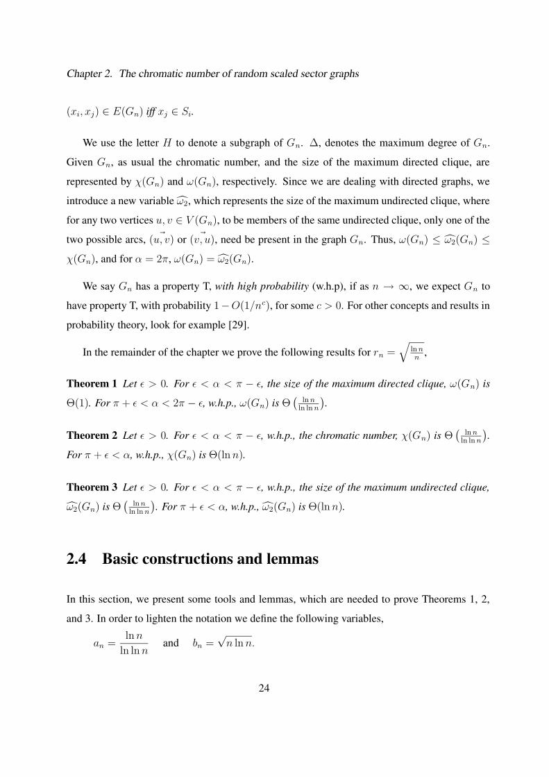
Figure 2.2: Angle partition for α > π + ε (a) classes B (b) directions associated to a class Bj
Recall, the orientation angle, βi, of every mote i is drawn uniformly at random (u.a.r) from
(0, 2π]. Many of the proofs in this chapter require partitioning the orientation angle into classes.
Thus we define a partition B of the orientation angle as follows.
Definition 2 Let ε be a constant (depending on α), such that α = π + ε, for 0 < ε < π. A Bpartition, is a partition of the region 2π into B classes, each of length ε− 2ε∗, with ε∗ a constant
chosen such that ε > 2ε∗ (see Figure 2.2). All motes i such that βi fall whose the same range will
belong to the same class. More specifically, for any 1 < j ≤ B, the class Bj is defined as the
class of motes whose bisectrix falls between (− 32+ j)ε− (2j− 3)ε∗ and (−1
2+ j)ε− (2j− 1)ε∗.
Notice B = d 2πε−2ε∗e, so B ∈ Z.
Throughout this chapter, when we refer to the dissection S of [0, 1]2, we mean a partition
of [0, 1]2 into nln n
squares, each one of size rn × rn. Also, in this chapter we make use of the
following three lemmas.
Lemma 1 ([24]) If n motes are distributed u.a.r. on [0, 1]2, w.h.p. each of the squares in the
dissection S will contain Θ(ln n) motes.
Lemma 2 If n motes are distributed u.a.r. on [0, 1]2, w.h.p. every square in the dissection S will
contain at most 3 ln n motes.
25
Chapter 2. The chromatic number of random scaled sector graphs
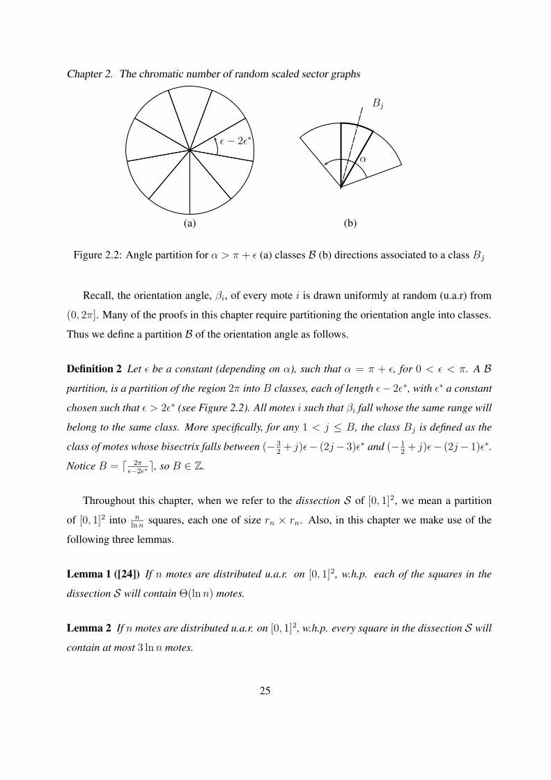
(a) (b) (c)
Figure 2.3: The basic dissections of [0, 1]2 (a) S (b) horizontal subdivision (c) vertical subdivision
Lemma 3 Given the dissection S of [0, 1]2, divide each square of S into ln n rectangular regions
of size rn
ln n× rn (see Figure 2.3). Then, w.h.p. there exists at least one region Ri, which contains
(1− o(1))an
Bmotes from every class Bj ∈ B.
The first two lemmas can be established via Chernoff bounds and Boole’s inequality. In order
to prove the third lemma, we use an implication of Talagrand’s inequality, given in [28]:
Talagrand’s Inequality Let X be a non-negative random variable, not identically 0, which is
determined by n independent trials L1, ...., Lm, and satisfying the following for some b,r > 0:
1. Changing the outcome of any one trial can affect X by at most b,
2. for any s, if X ≥ s there is a set of < rs trials whose outcomes certify that X ≥ s.
Then, for any 0 ≤ l ≤ E [X], P(|X − E [X]| > l + 60b
√rE [X]
)≤ 4e−l2/8b2rE[X].
Proof of Lemma 3 In order to prove Lemma 3 we make use of the following fact. If n balls
are dropped into n bins, w.h.p. at least one bin contains an = ln n/ ln ln n balls. Notice by
construction the number of regions in [0, 1]2is nln n
ln n = n, since the n motes are distributed
u.a.r. on [0, 1]2, by a balls-and-bins argument, there is a region Ri, which w.h.p. contains
an = ln n/ ln ln n motes. Let Xj be a random variable counting the number of motes in Ri
26

Chapter 2. The chromatic number of random scaled sector graphs
which are in class Bj . Then E [Xj] = an/B. To complete the proof of Lemma 3 we show via
Talagrand’s inequality the random variable Xj is concentrated around its expectation. First note,
Xj is determined by the m = (1 − o(1))an/B trials specifying β1, . . . , βm. Also changing
the outcome of any one βl, 1 ≤ l ≤ m, can affect Xj by at most one, and in order to certify
Xj ≥ s, only the outcomes of s trials (the s βl’s which fall in that class) are required. Thus the
conditions of Talagrand’s inequality are satisfied with b, r = 1. Hence by Talagrand’s inequality
and Boole’s inequality, w.h.p. every class contains (1− o(1))an/B motes. 2
2.5 Proof of Theorem 1
2.5.1 α < π − ε
Proof When α < π − ε the vertices of any clique must form a convex polygon. This can be
proved by first noting that in every clique of size three, the three points cannot be collinear, and
proceeding inductively. Let |V | represent the number of vertices in any clique. Since the sum of
the angles of a convex polygon is (|V |−2)π, we have |V |α ≥ (|V |−2)π, thus ω(Gn) ≤⌊
2ππ−α
⌋.
2
2.5.2 α > π + ε
Proof • First we establish the lower bound, by proving a certain sufficient configuration of
motes exists (w.h.p.). Consider the S partition of [0, 1]2. Subdivide each small square into ln n
equal (in terms of area) vertical regions (one can imagine drawing ln n equally spaced vertical
lines). By Lemma 3, there is a vertical region Ri w.h.p. containing (1− o(1)) an
Bmotes who are
members of the class B1, i.e. the bisectrix of these motes is between − 12ε + ε∗ and 1
2ε − ε∗ .
Let M1 be the set of these motes (in class B1) in Ri. Further subdivide the region Ri into an/B
cells, each cell a rectangle of width 1bn
and height Brn
an, see Fig. 2.4. Let Y be a random variable
27
Chapter 2. The chromatic number of random scaled sector graphs
counting the number of cells containing at least one vertex from M1, then E [Y ] = (1− 1e)an/B as
n→∞, and as in the proof of Lemma 3, one can show Y is concentrated around its expectation
by applying Talagrand’s inequality. Thus w.h.p there are at least (1 − ( 1e
+ o(1)))an/B cells
containing at least one mote from M1. Consider a mote m from the set M1, due to its orientation
angle, it will have an arc with any mote m′ which is an cell more than a specific distance, l,
and within distance rn in either direction, up or down from itself. Where l depends on the exact
orientation angle of the mote m, and the location of the two motes, m and m′ in their respective
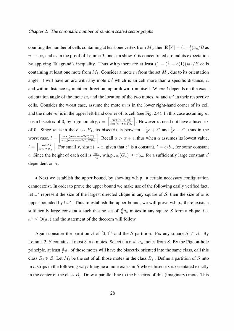
cells. Consider the worst case, assume the mote m is in the lower right-hand corner of its cell
and the mote m′ is in the upper left-hand corner of its cell (see Fig. 2.4). In this case assuming m
has a bisectrix of 0, by trigonometry, l =⌈
cos((α−π)/2)sin((α−π)/2)bn
⌉. However m need not have a bisectrix
of 0. Since m is in the class B1, its bisectrix is between − 12ε + ε∗ and 1
2ε − ε∗, thus in the
worst case, l =⌈
cos((α−π−ε+2ε∗)/2)sin((α−π−ε+2ε∗)/2)bn
⌉. Recall α > π + ε, thus when α assumes its lowest value,
l =⌈
cos(ε∗)sin(ε∗)bn
⌉. For small x, sin(x) ∼ x, given that ε∗ is a constant, l = c/bn, for some constant
c. Since the height of each cell is Brn
an, w.h.p., ω(Gn) ≥ c′an, for a sufficiently large constant c′
dependent on α.
• Next we establish the upper bound, by showing w.h.p., a certain necessary configuration
cannot exist. In order to prove the upper bound we make use of the following easily verified fact,
let ω∗ represent the size of the largest directed clique in any square of S , then the size of ω is
upper-bounded by 9ω∗. Thus to establish the upper bound, we will prove w.h.p., there exists a
sufficiently large constant d such that no set of dB
an motes in any square S form a clique, i.e.
ω∗ ≤ Θ(an) and the statement of the theorem will follow.
Again consider the partition S of [0, 1]2 and the B-partition. Fix any square S ∈ S . By
Lemma 2, S contains at most 3 ln n motes. Select u.a.r. d · an motes from S. By the Pigeon-hole
principle, at least dB
an of those motes will have the bisectrix oriented into the same class, call this
class Bj ∈ B. Let Mj be the set of all those motes in the class Bj . Define a partition of S into
ln n strips in the following way: Imagine a mote exists in S whose bisectrix is orientated exactly
in the center of the class Bj . Draw a parallel line to the bisectrix of this (imaginary) mote. This
28

Chapter 2. The chromatic number of random scaled sector graphs
(parallel) line will be the orientation of the strips. Cover S with ln n rectangular strips parallel to
the orientation (see Figure 2.5). For example, in the case where these motes belong to the class
B1, the rectangular strips will be parallel to the sides of S. Note by construction, in this partition
of S, the optical sensors of all the motes in the class Mj look in the same approximate direction.
Thus for these motes to be a part of the same clique every mote must see all the other motes
along some specified direction, and we will show w.h.p. this will not be the case.
Before we continue with the remainder of the proof we need to establish the following lemma.
Lemma 4 For a sufficiently large but constant d, any set of dB
an motes, will (w.h.p.) occupy at
least (ln n)9/10 strips.
Proof First we upperbound the area of any strip. The maximum length any strip can have is
rn
√2 since we are considering a [rn × rn] square S. The maximum width any strip can have is
√2rn/ ln n (this occurs when the orientation of strips is parallel to the diagonal of S). Thus the
area of the largest strip is bounded above by
√2rn/ ln n× rn
√2 =
2
n.
Now we upperbound the probability that any set of (ln n)9/10 of the strips will contain dB
an
motes in S.
Any set of (ln n)9/10 strips by the above upperbound have total area at most 2 ln n9/10
n. Thus
the area of any set of (ln n)9/10 strips divided by the area of S is at most 2(ln n)1/10 , which is the
probability that any given mote in S falls in the (ln n)9/10 strips.
Let p1 be the probability that in any small square, a set of least dB
an motes falls in at most
(ln n)9/10 strips. W.h.p. no small square has more than 3 ln n motes, thus the number of ways to
choose a set of dB
an motes from 3 ln n motes is(
3 ln ndB
an
)< n3.
29
Chapter 2. The chromatic number of random scaled sector graphs
Moreover, as there are n/ ln n small squares and at most n ways to choose (ln n)9/10 strips out
of ln n strips, by Boole’s inequality,
p1 ≤ n5
(2
(ln n)1/10
) d ln nB ln ln n
≤ n6
(1
eln(ln n)
10danB
)= n6e−
d ln n10B .
Therefore, as n→∞, a sufficiently large constant d can be chosen such that p1 → 0.
2
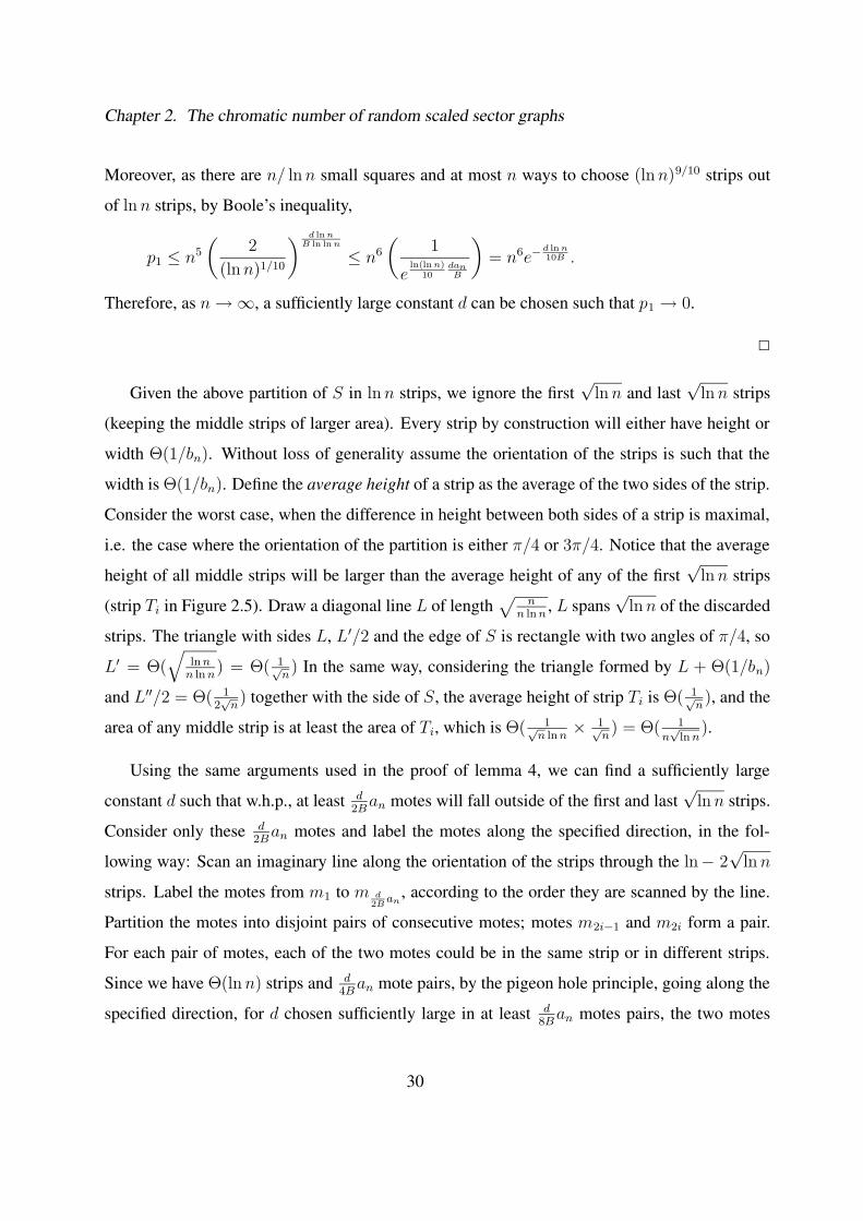
Given the above partition of S in ln n strips, we ignore the first√
ln n and last√
ln n strips
(keeping the middle strips of larger area). Every strip by construction will either have height or
width Θ(1/bn). Without loss of generality assume the orientation of the strips is such that the
width is Θ(1/bn). Define the average height of a strip as the average of the two sides of the strip.
Consider the worst case, when the difference in height between both sides of a strip is maximal,
i.e. the case where the orientation of the partition is either π/4 or 3π/4. Notice that the average
height of all middle strips will be larger than the average height of any of the first√
ln n strips
(strip Ti in Figure 2.5). Draw a diagonal line L of length√
nn ln n
, L spans√
ln n of the discarded
strips. The triangle with sides L, L′/2 and the edge of S is rectangle with two angles of π/4, so
L′ = Θ(√
ln nn ln n
) = Θ( 1√n) In the same way, considering the triangle formed by L + Θ(1/bn)
and L′′/2 = Θ( 12√
n) together with the side of S, the average height of strip Ti is Θ( 1√
n), and the
area of any middle strip is at least the area of Ti, which is Θ( 1√n ln n
× 1√n) = Θ( 1
n√
ln n).
Using the same arguments used in the proof of lemma 4, we can find a sufficiently large
constant d such that w.h.p., at least d2B
an motes will fall outside of the first and last√
ln n strips.
Consider only these d2B
an motes and label the motes along the specified direction, in the fol-
lowing way: Scan an imaginary line along the orientation of the strips through the ln− 2√
ln n
strips. Label the motes from m1 to m d2B
an, according to the order they are scanned by the line.
Partition the motes into disjoint pairs of consecutive motes; motes m2i−1 and m2i form a pair.
For each pair of motes, each of the two motes could be in the same strip or in different strips.
Since we have Θ(ln n) strips and d4B
an mote pairs, by the pigeon hole principle, going along the
specified direction, for d chosen sufficiently large in at least d8B
an motes pairs, the two motes
30

Chapter 2. The chromatic number of random scaled sector graphs
in the pair, will be within 2 ln ln n strips of each other. Now in order for these motes to be part
of the same clique, in each pair both motes must see each other. Without loss of the generality
assume the orientation of the strips is parallel to the side of S, such that every mote can see every
other mote to its right. Thus at least one of the necessary arcs is present. For the other arc to
be present the right-most mote (in the mote pair) must see the mote to its left. Since the strips
in question have a width of at least Θ(
1√n
), the horizontal coordinates of both points are drawn
u.a.r. from(0, Θ
(1√n
)]. Thus in order to compute the probability of this event we will consider
two disjoint cases.
Case one, the horizontal coordinates of at least one mote is in the interval(0, 1
(ln n)1/10√
n
]. In
that case we will assume with probability one, the right mote see’s the left mote. The probability
of case one occurring is Θ(
1(ln n)1/10
).
Case two, the horizontal coordinates of both motes is > 1(ln n)1/10
√n
. In this case since ε∗ is
a constant, the maximum area a mote see’s of any strip which is within 2 ln ln n strips of it (in
a specified direction) is at most Θ(1/(nan)). This follows, since the region of any one strip the
mote see’s has at most a width of Θ(rn/an) and height Θ(1/bn) (given the strip in question is
within 2 ln ln n strips of the mote). Now the left-most mote (in the pair) must fall in a strip. Also
(since we are conditioning on being in case two), its horizontal coordinate is drawn u.a.r. from
an interval of length > 1(ln n)1/10
√n
. Thus since every strip has height of Θ(1/bn), conditioning
on the particular strip the left-most mote falls into, the left-most mote falls u.a.r. into an area
> Θ(
1n(ln n)6/10
). Thus the probability the right mote see’s the left mote, conditioned on case
two occurring, is at most Θ(
1(ln n)4/10
). Thus the probability the right mote see’s the left mote is
at most,
Θ
(1
(ln n)1/10
)+ Θ
(1
(ln n)4/10
)= Θ
(1
(ln n)1/10
).
Since for every pair of motes these events are independent of each other (because only disjoint
pairs are being considered), the probability for every pair of motes, both motes see each other is
31

Chapter 2. The chromatic number of random scaled sector graphs
≤ Θ
(1
(ln n)1/10
) d ln n8B ln ln n
.
Let p2 denote the probability in any square S in S , there is a clique of size d · an or greater.
Since (w.h.p.) in any square S we have at most n3 sets of size d·an or greater, and n/ ln n squares
in S , by Boole’s inequality
p2 ≤ n4Θ
(1
(ln n)1/10
) d ln n8B ln ln n
≈ n4e−d ln n80B .
Therefore, there is a sufficiently large constant d such that p2 → 0, and thus w.h.p., ω∗ ≤ Θ(an).
2
2.5.3 α = 2π
For α = 2π, a random sector graph is equivalent to a random disk graph. For a random disk graph
it is already known w.h.p., ω(Gn) is Θ(ln n) [29]. However, this fact can be directly verified, as
above, by partitioning the [0, 1]2 unit square into c nln n
regions, and bounding (w.h.p.) the number
of motes in any region. Thus the value of ω(Gn), for the particular value of rn considered in this
chapter, exhibits two transitions, one at π + ε, the other at 2π.
2.6 Proof of Theorem 2
2.6.1 α > π + ε
Proof Partition the unit square into 2n/ ln n,[
rn√2× rn√
2
]small squares, call this a S∗ partition.
Observe that all the motes in any small square are at most a distance of rn apart. Since there
are 2n/ ln n squares and n motes, by the pigeon hole principle at least one of the small squares
32
Chapter 2. The chromatic number of random scaled sector graphs
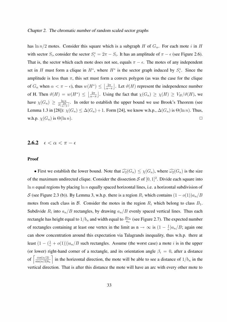
has ln n/2 motes. Consider this square which is a subgraph H of Gn. For each mote i in H
with sector Si, consider the sector S∗i = 2π − Si. It has an amplitude of π − ε (see Figure 2.6).
That is, the sector which each mote does not see, equals π − ε. The motes of any independent
set in H must form a clique in H∗, where H∗ is the sector graph induced by S∗i . Since the
amplitude is less than π, this set must form a convex polygon (as was the case for the clique
of Gn when α < π − ε), thus w(H∗) ≤⌊
2πα−π
⌋. Let ϑ(H) represent the independence number
of H. Then ϑ(H) = w(H∗) ≤⌊
2πα−π
⌋. Using the fact that χ(Gn) ≥ χ(H) ≥ VH/ϑ(H), we
have χ(Gn) ≥ ln n2b 2π
α−πc . In order to establish the upper bound we use Brook’s Theorem (see
Lemma 1.3 in [28]): χ(Gn) ≤ ∆(Gn) + 1. Form [24], we know w.h.p., ∆(Gn) is Θ(ln n). Thus,
w.h.p. χ(Gn) is Θ(ln n). 2
2.6.2 ε < α < π − ε
Proof
• First we establish the lower bound. Note that ω2(Gn) ≤ χ(Gn), where ω2(Gn) is the size
of the maximum undirected clique. Consider the dissection S of [0, 1]2. Divide each square into
ln n equal regions by placing ln n equally spaced horizontal lines, i.e. a horizontal subdivision of
S (see Figure 2.3 (b)). By Lemma 3, w.h.p. there is a region Ri which contains (1− o(1))an/B
motes from each class in B. Consider the motes in the region Ri which belong to class B1.
Subdivide Ri into an/B rectangles, by drawing an/B evenly spaced vertical lines. Thus each
rectangle has height equal to 1/bn and width equal to Brn
an(see Figure 2.7). The expected number
of rectangles containing at least one vertex in the limit as n → ∞ is (1 − 1e)an/B; again one
can show concentration around this expectation via Talagrands inequality, thus w.h.p. there at
least (1 − (1e
+ o(1)))an/B such rectangles. Assume (the worst case) a mote i is in the upper
(or lower) right-hand corner of a rectangle, and its orientation angle βi = 0, after a distance
of⌈
cos(α/2)sin(α/2)bn
⌉in the horizontal direction, the mote will be able to see a distance of 1/bn in the
vertical direction. That is after this distance the mote will have an arc with every other mote to
33

Chapter 2. The chromatic number of random scaled sector graphs
its right within a distance of rn in the rectangle in question. Repeating the same arguments as in
the case of ω(Gn) (which we omit in the interest of space), one can establish, w.h.p., ω2(Gn) is
at least d · an, where d is some constant dependent on α.
• Next we establish the upper bound. Consider the dissection S on [0, 1]2. Let χ∗ represent
the largest chromatic number of any square S in S , then it is easily verifiable χ(Gn) is upper-
bounded by 9χ∗, thus in order to upperbound χ(Gn), we upperbound χ∗.
Again fix a square S in S and consider the partition B. By the Pigeon hole principle, at least
one class Bj will contain dB
an motes in S all them oriented in almost the same direction. Let
Mj be the set of all such motes. Define a partition of S into ln n strips in the following way.
Imagine there exists a mote in S, whose bisectrix falls exactly in the center of the class Bj . Draw
a line perpendicular to the bisectrix of this (imaginary) mote. This perpendicular line will be
the orientation of the strips (note in the case of ω(Gn), Theorem 1, a different orientation was
used). Partition S into ln n strips parallel to the orientation (see Figure 2.8), in this partition
of S, all the motes in Mj look in the same approximate direction. We wish to prove that for a
sufficiently large constant d, w.h.p. every set of dB
an motes contains an independent set of size
at least 1/3 ln ln n.
Using similar arguments as in Section 1, one can show w.h.p. at least d2B
an motes fall into
a strip having average height > Θ(
1√n
). Thus we only consider motes falling into the strips
having average height > Θ(
1√n
). Next, we will order these motes going along the specified
direction. For example assume the specified direction is going left to right. Then we label the
leftmost mote, 1, the second leftmost mote, 2, and so on. Next we partition the d2B
an motes intod·an
2B ln ln nclasses. Each class C will contain ln ln n motes. Again imagine that we are going from
left to right, then class one will contain mote1 to moteln ln n, and class two will contain the next
ln ln n motes. Now again by the pigeon hole principle at least one half of these classes occupy
at most 2 ln n2B ln ln nd·an
strips. For d sufficiently large this means at least d·an
4B ln ln nclasses occupy at
most 2 ln ln n strips.
34
Chapter 2. The chromatic number of random scaled sector graphs
Now we consider one class of these motes, say class one. We define two edges to be inde-
pendent of each other if they have no endpoints in common. Thus the edges a-b and b-c are not
independent, whereas the edges a-b and c-d are independent (where a, b, c, and d are vertices).
Lemma 5 For any class C of ln ln n motes, if the largest independent edge set is less than
1/3 ln ln n, then there exits an independent set of size 1/3 ln ln n or greater.
Proof This follows from the fact that the size of the vertex cover is at most 2 times the size
of the maximal independent edge set with minimum cardinality. More specifically, assume the
largest set of independent edges in C is ≤ 1/3 ln ln n. Remove all the endpoints (along with
any of their edges) from the graph. Since this was the largest independent set of edges (i.e. it is
trivially maximal), any other edge not in this set must be dependent relative to some edge in this
set (otherwise we would have included it in the set). Thus by removing all the endpoints in this
set (the one with the most independent edges) we have deleted all the edges in this subgraph (i.e.
in the class in question). Each independent edge has two endpoints. The largest such set is by
assumption at most 1/3 ln ln n. Thus we have removed at most 2/3 ln ln n motes (i.e. vertices).
The class to begin with had ln ln n motes. Thus we are left with at least 1/3 ln ln n motes. And
all the edges have been removed, hence these 1/3 ln ln n motes form an independent set and the
lemma is proved. 2
Define p3 to be the probability in any one particular class an independent edge set of size
1/3 ln ln n or greater exists. First we will restrict ourselves to classes C ′ which occupy 2 ln ln n
strips or less (at least half of the classes are of this type). Thus every mote is within 2 ln ln n
strips of any other mote in the class. In order for two motes to share an edge, one mote must
see the other going along the specified (in our case going from left to right) direction. There are(ln ln n
2
)< (ln ln n)2 possible total edges in the class. Recalling the strips have average height of
at least Θ(
1√n
), the probability any one edge is present is < Θ
(ln ln n
(ln n)1/2
). The probability any
edge exists is independent of any other edge existing (since we are considering independent edge
sets). The cardinality of the largest independent edge set is ≤ 1/2 ln ln n, thus the total number
35

Chapter 2. The chromatic number of random scaled sector graphs
of ways to chose an independent set greater than 1/3 ln ln n is < ln ln nln ln n. Hence by Boole’
inequality for d sufficiently large,
p3 ≤ Θ
(ln ln nln ln n
(ln ln n
(ln n)1/2
)1/3 ln ln n)≤ 1
(ln n)4/10
1/4 ln ln n
≡ e−d ln n40B .
Let p4 denote the probability in any small square a set with d · an motes does not have an inde-
pendent set of size 1/3 ln ln n or greater. There are at most (w.h.p.) n3 ways to choose a set of
d · an motes in any small square. We are considering d·an
4B ln ln nclasses of motes, i.e. all the classes
which occupy at most 2 ln ln n strips. No two classes have any motes in common, thus they are
independent of each other. And we have n/ ln n small squares, so for d sufficiently large, by
Boole’s inequality
p4 ≤ n4e−(1/10(ln ln n)2)
(d ln n
4B(ln ln n)2
)
≡ n4e−d ln n40B .
Therefore, there exists a sufficiently large constant d such that p4 → 0.
Thus w.h.p., in every small square any set of d · an motes, has an independent set of size
at least 1/3 ln ln n. Now take any small square, and keep on choosing independent sets of size
1/3 ln ln n. Assign all the motes in the same independent set the same color. When there are less
than d · an motes left, assign all the remaining motes a different color. Thus we have colored all
the motes in any small square (w.h.p.) with at most 3 ln n−d·an
1/3 ln ln n+d ·an colors. Since the chromatic
number of the graph (χ(Gn)), is at most a constant times this amount, w.h.p. χ(Gn) = O(
ln nln ln n
).
Combining with our lower bound, we have χ(Gn) is, w.h.p., Θ(
ln nln ln n
). 2
2.7 Proof of Theorem 3
2.7.1 α > π + ε
Proof First we prove for α > π + ε, w.h.p., ω2 ≥ Θ(ln n). Again, consider the dissection Sof [0, 1]2. By the pigeon hole principle at least one of the squares has ln n/2 motes. Further all
36
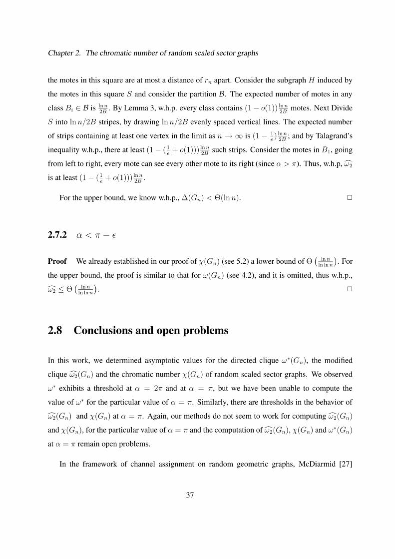
Chapter 2. The chromatic number of random scaled sector graphs
the motes in this square are at most a distance of rn apart. Consider the subgraph H induced by
the motes in this square S and consider the partition B. The expected number of motes in any
class Bi ∈ B is ln n2B
. By Lemma 3, w.h.p. every class contains (1− o(1)) ln n2B
motes. Next Divide
S into ln n/2B stripes, by drawing ln n/2B evenly spaced vertical lines. The expected number
of strips containing at least one vertex in the limit as n → ∞ is (1 − 1e) ln n
2B; and by Talagrand’s
inequality w.h.p., there at least (1− ( 1e+ o(1))) ln n
2Bsuch strips. Consider the motes in B1, going
from left to right, every mote can see every other mote to its right (since α > π). Thus, w.h.p, ω2
is at least (1− ( 1e
+ o(1))) ln n2B
.
For the upper bound, we know w.h.p., ∆(Gn) < Θ(ln n). 2
2.7.2 α < π − ε
Proof We already established in our proof of χ(Gn) (see 5.2) a lower bound of Θ(
ln nln ln n
). For
the upper bound, the proof is similar to that for ω(Gn) (see 4.2), and it is omitted, thus w.h.p.,
ω2 ≤ Θ(
ln nln ln n
). 2
2.8 Conclusions and open problems
In this work, we determined asymptotic values for the directed clique ω∗(Gn), the modified
clique ω2(Gn) and the chromatic number χ(Gn) of random scaled sector graphs. We observed
ω∗ exhibits a threshold at α = 2π and at α = π, but we have been unable to compute the
value of ω∗ for the particular value of α = π. Similarly, there are thresholds in the behavior of
ω2(Gn) and χ(Gn) at α = π. Again, our methods do not seem to work for computing ω2(Gn)
and χ(Gn), for the particular value of α = π and the computation of ω2(Gn), χ(Gn) and ω∗(Gn)
at α = π remain open problems.
In the framework of channel assignment on random geometric graphs, McDiarmid [27]
37
Chapter 2. The chromatic number of random scaled sector graphs
studied the value of the chromatic number for two types of random geometric graphs. In the
case of sparse graphs, defined as r2nn/ ln n → 0, (i.e. the average degree is o(ln n)), in prob-
ability χ/ω → 1. In the case of dense graphs, defined as r2nn/ ln n → ∞, in probability
χ/ω → 2√
3/π ∼ 1.103. McDiarmid leaves as open the problem of computing the chromatic
number of random geometric graphs for which r2nn/ ln n tends to a constant c as n → ∞. No-
tice this radii is the one considered in this chapter for random scaled sector graphs. Thus the
work of McDiarmid suggests two lines for further investigation; the asymptotic evaluation of
χ(Gn)/ω2(Gn) when r2nn/ ln n tends to a constant c, and the study of χ(Gn) and ω2(Gn) for the
particular cases of sparse and dense random scaled sector graphs.
38
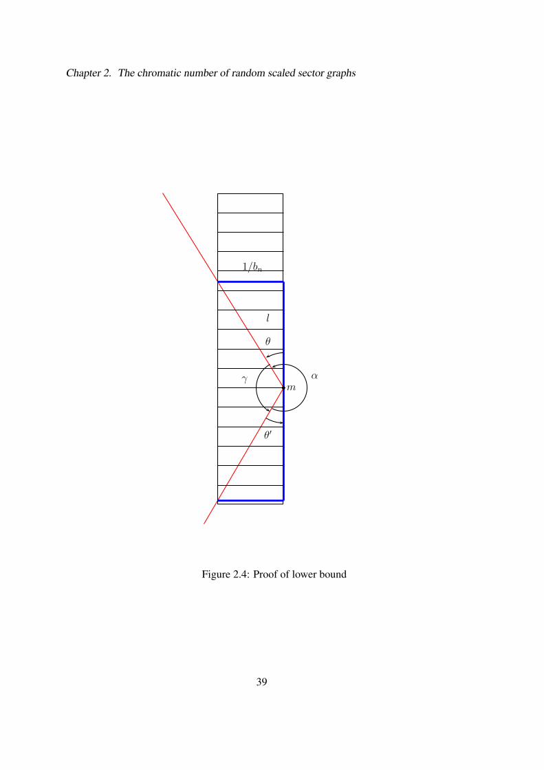
Chapter 2. The chromatic number of random scaled sector graphs
θ
θ′
αγ
1/bn
l
m
Figure 2.4: Proof of lower bound
39

Chapter 2. The chromatic number of random scaled sector graphs
L ′L ′′
Ti 2/bn
L
L
L′/2
Figure 2.5: Partition of S by strips
S∗i
Si
Figure 2.6: Sector Si and complementary sector S∗i
40

Chapter 2. The chromatic number of random scaled sector graphs
α1/bn
m
Figure 2.7: Figure for the proof of 5.2
L ′L ′′
Ti 2/bn
L
Figure 2.8: Partition of S in the prove 5.2
41
Chapter 3
Counting Connected Graphs and
Hypergraphs via the Probabilistic Method
3.1 Acknowledgements
I would like to thank Amin Coja-Oghlan and Cristopher Moore. The work in this chapter was
done jointly with them, a preliminary version of which appeared in [35].
3.2 Introduction and Results
A d-uniform hypergraph H consists of a set V of vertices and a set E of edges, which are subsets
of V of cardinality d. For instance, a 2-uniform hypergraph is just a graph. A vertex w is
reachable in H from a vertex v if either v = w or there is a sequence e1, . . . , ek of edges such
that v ∈ e1, w ∈ ek, and ei ∩ ei+1 6= ∅ for i = 1, . . . , k − 1. Of course, reachability in H is an
equivalence relation. The equivalence classes are the components of H , and H is connected if
there is only one component.
42

Chapter 3. Counting Connected Graphs and Hypergraphs via the Probabilistic Method
Connectedness is perhaps the most basic property of graphs and hypergraphs, and therefore
estimating the number of connected graphs or hypergraphs with a given number of vertices and
edges is a fundamental combinatorial problem. In most applications, one is interested in asymp-
totic results, where the number of vertices/edges tends to infinity. The main result in this chapter
is a formula for the asymptotic number of connected d-uniform hypergraphs; or, equivalently, an
estimate of the probability that a random d-uniform hypergraph is connected. Our results hold
up to a constant multiplicative factor. We study both a model Hd(n,m) in which the number of
vertices and edges is fixed, and a binomial model Hd(n, p) in which each possible edge appears
with probability p independently. In the latter case we also calculate the expected number of
edges given that the hypergraph is connected. Furthermore, we obtain a simple algorithm for
generating a connected hypergraph uniformly at random.
For the special case of graphs, i.e., for d = 2, the results we present in this chapter (and, in
some cases, stronger results) are already known. By contrast, little has previously been known
about d-uniform hypergraphs where d ≥ 3, although a few papers deal with the component
structure of random hypergraphs. We will discuss related work in Section 3.2.3 after presenting
our main results.
We obtain our results using a new probabilistic approach. Rather than using powerful tech-
niques of enumerative combinatorics such as generating functions, our calculations are for the
most part elementary, and just rely on the fact that each connected (hyper)graph of a given order
and size is equally likely to occur as the “giant component” of a larger one. We believe that
this approach is of interest in its own right, and that similar ideas can be applied to a number of
further problems in combinatorics and random (hyper)graph theory.
3.2.1 Results
Throughout, we will consider d-uniform hypergraphs where d ≥ 2 is a fixed integer. Given a
hypergraph H = (V,E), its order is its number of vertices |V |, and its size is its number of edges
43
Chapter 3. Counting Connected Graphs and Hypergraphs via the Probabilistic Method
|E|. The degree of a vertex v ∈ V is the number of edges e ∈ E such that v ∈ e. Hence, if H
is d-uniform, its average degree is d|E|/n, Observe that if a d-uniform hypergraph is connected,
then its average degree is at least (1− n−1) dd−1
.
Two natural random models of hypergraphs present themselves. In Hd(n,m), we select one
of the((n
d)m
)sets of m possible edges uniformly at random. In Hd(n, p), each of the
(nd
)edges
appears independently with probability 0 ≤ p ≤ 1, in which case the expected number of edges
is(
nd
)p and the expected average degree is
(n−1d−1
)p. Thus we will compare Hd(n,m) where
m = cn/d with Hd(n, p) where p = c/(
n−1d−1
). While these two models are interchangeable in
many respects, we will show that their probabilities of connectedness differ by an exponential
factor if the average degree is constant. We say that Hd(n,m) or Hd(n, p) has a certain property
with high probability (w.h.p.) if the probability that the property holds tends to 1 as n→∞.
The following theorem determines the asymptotic probability of connectedness of Hd(n,m),
or equivalently the number of connected d-uniform hypergraphs, up to a constant factor in the
regime where the average degree is d/(d− 1) + Ω(1) < c = o(ln n). We let cd(n,m) signify the
probability that the random hypergraph Hd(n,m) is connected, and in addition Cd(n,m) denotes
the number of connected d-uniform hypergraphs of order n and size m.
Theorem 1 Let c0 > d/(d − 1) be a number independent of n. Then there exist numbers C0,
C ′0 that depend only on c0 such that for all c0 ≤ c = c(n) = o(ln n) the following holds. The
equation
1− a = exp
(−ca · 1− (1− a)d−1
1− (1− a)d
)(3.1)
has a unique solution a = a(c) in the interval (0, 1). Set m = cn/d. Then for all sufficiently
large n
C0Φd(c)n ≤ cd(n,m) = Cd(n,m)
((nd
)
m
)−1
≤ C ′0Φd(c)
n, where
Φd(c) = a1−c (1− a)(1/a)−1(1− (1− a)d
)c/d.
44

Chapter 3. Counting Connected Graphs and Hypergraphs via the Probabilistic Method
The next theorem gives an analogous result for Hd(n, p). We let cd(n, p) signify the proba-
bility that Hd(n, p) is connected.
Theorem 2 For each constant c0 > 0 there exists numbers C1, C′1 depending only on c0 such
that for all c0 ≤ c = c(n) = o(ln n) the following holds. Let p = c/(
n−1d−1
). Then the equation
1− a = exp
(−c · 1− (1− a)d−1
ad−1
)(3.2)
has a unique solution a in the interval (0, 1). For all sufficiently large n we have
C1Ψd(c)n ≤ cd(n, p) ≤ C ′
1cd(n, p), where Ψd(c) = a (1−a)(1/a)−1 exp
(c
d· 1− ad − (1− a)d
ad
).
For d = 2 the formula simplifies to Ψ2(c) = 1− exp(−c).
Note Hd(n, p) is exponentially more likely to be connected than Hd(n,m) if m =(
nd
)p.
The reason for this is that in Hd(n, p) the number of edges is a random variable: we can
think of Hd(n, p) as first choosing a number of edges m′ according to the binomial distribu-
tion Bin((
nd
), p), and then choosing a Hd(n,m′). Thus Hd(n, p) can boost its probability of
being connected by including a larger number m′ >(
nd
)p of edges. Indeed, given that Hd(n, p)
is connected, the conditional expectation of the number of edges will be significantly larger than(
nd
)p. Our next theorem quantifies this observation.
Theorem 3 Let c, a, and p be as in Theorem 2. Set γd(c) = c[1− (1− a)d
]a−d . Then the
expected number of edges of Hd(n, p) given that that Hd(n, p) is connected is nγd(c)/d + o(n),
so the expected average degree is γd(c) + o(1). For d=2, the formula simplifies to γ2(c) =
c · coth(c/2).
As c→∞, γd(c) ∼ c, since connectedness becomes a less unusual condition as c increases. As
c→ 0, γd(c)→ d/(d− 1), the minimum average degree required for connectivity.
Theorem 1 addresses the combinatorial problem of estimating the number of connected hy-
pergraphs. But there is also a corresponding algorithmic problem: can we sample a connected
45

Chapter 3. Counting Connected Graphs and Hypergraphs via the Probabilistic Method
hypergraph of a given order and size efficiently uniformly at random? We answer this question
in the affirmative.
Theorem 4 Let c0 > d/(d − 1) be fixed, let c0 ≤ c = o(ln n), and let m = cn/d. There is a
randomized algorithm that samples a connected hypergraph of order n and size m uniformly at
random in expected time O(n1/2m3/2).
One ingredient of the proofs of Theorems 1–4 is a result on the component structure of
random hypergraphs Hd(n,m) and Hd(n, p). Suppose that the average degree c = dm/n (resp.
c =(
n−1d−1
)p) is a constant greater than 1/(d − 1). Then, just as for graphs (cf. [34, 39]), w.h.p.
there is a unique giant component of order Ω(n) in Hd(n, p), while all other components are of
order O(ln n). To prove Theorems 1–4, it is crucial to have a rather tight estimate on the order
and size of the giant component. Since these considerations may be of independent interest, we
state the result as a theorem. For a hypergraph H we let N (H) (resp.M(H)) denote the largest
order (size) of a component of H .
Theorem 5 Let p = c(
n−1d−1
)−1and m =
(nd
)p = cn/d.
1. If there is a constant c0 < (d− 1)−1 such that c ≤ c0, then w.h.p. we have N (Hd(n, p)) =
O((1− (d− 1)c0)−2 ln n).
2. Suppose that c0 > (d − 1)−1 is a constant, and that c0 ≤ c = o(ln n). There is a unique
number 0 < a = a(c) < 1 such that 1 − a = exp[c((1− a)d−1 − 1)
]. Set b = b(c) =
1− (1− a)d. Then we have
1− a = exp(−Θ(c)), (3.3)
E [N (Hd(n, p))] = an + no(1), E [M(Hd(n, p))] = bm + no(1), (3.4)
Var(N (Hd(n, p))) ∼a(1− a)
[1 + ((d− 1)c− 1)
∑d−2i=1 (1− a)j
]
(1− c(d− 1)(1− a)d−1)2· n. (3.5)
46
Chapter 3. Counting Connected Graphs and Hypergraphs via the Probabilistic Method
Furthermore, with probability ≥ 1− n−10 there is precisely one component of order (1 +
o(1))an in Hd(n,m), while all other components have order O(c((d− 1)c− 1)−2 ln n). In
addition, with probability 1− exp(−nΩ(1)) the number of isolated vertices is n exp(−c) +
o(n9/10). Finally, for each ε > 0 there is a constant Cε > 0 such that
P[|M(Hd(n, p))− bm| ≤ Cεn
d/2p1/2]≥ 1− ε. (3.6)
3.2.2 Techniques and Overview
While most of the previous work on counting connected (hyper)graphs relies on rather heavy ma-
chinery from enumerative combinatorics, our approach is quite different and employs only rela-
tively simple probabilistic techniques. For instance, the basic idea behind the proof of Theorem 1
is as follows. Suppose that p = c/(
n−1d−1
)for some c > 1/(d− 1), and let a, b be as in Theorem 5.
Then, by Theorem 5, w.h.p. there is a unique giant component in Hd(n, p), which—conditioned
on its order and size—is a uniformly random connected hypergraph. To prove Theorem 1, we
derive an explicit formula that expresses the number Cd(ν, µ) of connected hypergraphs of order
ν = an and size µ = bm in terms of the probability χ(ν, µ) that the giant component of Hd(n, p)
has precisely order ν and size µ. Then, we prove that χ(ν, µ) = Θ((1− a)bm)−1/2 to obtain the
estimate of Cd(ν, µ) stated in Theorem 1.
To compute χ(ν, µ), we expose the edges of Hd(n, p) in two rounds. In the first round we
include edges with probability p1 = (1 − ε)p independently, where ε > 0 is a sufficiently small
constant. In the second round we add further edges with probability p2, where p1+p2−p1p2 = p,
so that the resulting hypergraph is distributed as Hd(n, p). As Theorem 5 yields the approximate
order and size of the giant component of the random hypergraph H1 = Hd(n, p1) generated in
the first round, to compute χ(an, bm) we just need to study the growth of the giant of H1 when
further edges are added with probability p2, i.e, with a fairly small probability.
The (somewhat technical) proof of Theorem 5 is based on the analogy between exploring
the components of a random hypergraph Hd(n, p) and a Galton-Watson branching process. This
47
Chapter 3. Counting Connected Graphs and Hypergraphs via the Probabilistic Method
analogy is well known for graphs, cf. [30, Chapter 10] and [39, Chapter 5]. While the basic
approach we use is the same as in [30, 39], we need to modify the previous techniques in three
respects.
• We generalize the branching processes considered in [30, 39] so that they describe explor-
ing the components of d-uniform hypergraphs rather than graphs.
• In [30, 39] it is shown via the branching process that the expected order and size of the
giant component of H2(n, p) is (1 + o(1))an (resp. (1 + o(1))bm). By comparison, (3.4)
gives the order/size of the giant up to an additive error of no(1). To obtain these more
precise statements, more involved technical estimates are necessary.
• Additionally, we also use the branching process to determine the variance of the number of
vertices in the giant component and the variance of the number of edges outside the giant
component.
In Theorems 1–5 we assume that c = o(ln n). Although our arguments also apply if c =
Ω(ln n), the assumption c = o(ln n) is convenient in order to avoid technical case distinctions.
Moreover, if c > (1+ε) ln n for an arbitrarily small but constant ε > 0, then w.h.p. both Hd(n, p)
and Hd(n,m) are connected, i.e., cd(n,m) = cd(n, p) = 1 (the proof given in for the case d = 2
in [34, Section 7.1] carries over to larger d without essential modifications).
The chapter is organized as follows. In Section 3.3 we introduce some notation and make a
few preliminary remarks. Then, in Section 3.4 we derive the formula for Cd(ν, µ) in terms of
χ(ν, µ). In addition, we also obtain a similar formula for cd(ν, p) to prove Theorem 2, and we
prove Theorem 4. Furthermore, in Section 3.5, we determine χ(ν, µ). Thus, Sections 3.4–3.5
present the main ideas of this chapter. Then, in Section 3.6 we show how Theorem 1 implies
Theorem 3. Finally, Section 3.7 deals with the proof of Theorem 5.
48

Chapter 3. Counting Connected Graphs and Hypergraphs via the Probabilistic Method
3.2.3 Related Work
The asymptotic number of connected graphs with a given number of edges and vertices was
determined by Bender, Canfield, and McKay [32]. Their proof is based on generating functions,
and gives a stronger result than Theorem 1 in that it determines the number of connected graphs
up to a multiplicative factor 1 + o(1) instead of a constant. The same authors determined the
probability that a random graph G(n, p) = H2(n, p) is connected as well as the expected number
of edges of G(n, p) conditioned on connectedness [33], corresponding to the case d = 2 of
Theorems 2 and 3. Indeed, they even give the asymptotic distribution of the number of edges
conditioned on connectedness, not just its expectation. An algorithm for generating random
connected graphs (the case d = 2 of Theorem 4) immediately follows from the results in [32,
33]. Pittel and Wormald [45] presented an alternative approach based on enumerating graphs of
minimum degree 2 to derive improved versions of some of the results in [32, 33].
The basic idea of this chapter—expressing Cd(ν, µ) in terms of χ(ν, µ) and computing the
latter via probabilistic methods, cf. Section 3.2.2—is related to the work of Łuczak [42] on
bounding C2(ν, µ) with µ = (1 + o(1))ν. To bound C2(ν, µ) from above, Łuczak expresses the
expected number of components of G(n, p) = H2(n, p) of order ν and size µ in terms of C2(ν, µ).
Then, he points out that the expected number of such components is trivially bounded by n/ν,
thereby obtaining an upper bound on C2(ν, µ). The difference between Łuczak’s approach and
ours is that we actually determine the probability that Hd(n, p) has a component of order ν = an
and size µ = bm up to a constant factor, rather than using the trivial upper bound n/ν on the
number of such components. Moreover, we use the probabilistic argument to get both an upper
and a lower bound on Cd(ν, µ), while the lower bound given in [42] relies on different techniques
(e.g., on an explicit formula for the asymptotic number of 3-regular graphs).
O’Connell [43] showed that the probability c2(ν, p) that G(ν, p) is connected is Ψ2(νp)ν+o(ν)
(cf. the d = 2 case of Theorem 2). The proof relies on the fact that w.h.p. the giant component
of G(n, p) has order an + o(n) where 1− a = exp(−ac), 0 < a < 1 (cf. Theorem 5). However,
49

Chapter 3. Counting Connected Graphs and Hypergraphs via the Probabilistic Method
since O’Connell avoids computing the probability that the order of the giant component actually
equals ν = an, he only obtains the value of c2(ν, p) up to a factor of exp(o(ν)) (rather than a
constant factor as in Theorem 2).
Independently of us and simultaneously, van der Hofstad and Spencer [37] determined the
number C2(n,m) of connected graphs via probabilistic methods up to a factor 1 + o(1). The
basic ingredient to their analysis is a novel point of view of the branching process argument for
exploring the components of G(n, p). However, there seems to be no direct way to extend the
approach of [37] to hypergraphs.
The asymptotic order and size of the giant component of random graphs (the case d = 2
of Theorem 5) has been known since the pioneering work of Erdos and Renyi, cf. [34, 39] for
unified treatments. The distribution of the giant component was further investigated by several
researchers, cf. [31, 38, 44] and the monographs [34, 39].
In comparison to the case of graphs (d = 2), little is known for d-uniform hypergraphs with
d ≥ 3. Karonski and Łuczak [41] determined the number of connected hypergraphs of order n
and size m = n/(d − 1) + k where k = o(ln n/ ln ln n) (i.e., just above the number of edges
necessary for connectedness) up to a factor of 1 + o(1) via purely combinatorial techniques.
Since Theorem 1 addresses the case m = cn/d for c ≥ d/(d− 1) + Ω(1), our results and those
of [41] are incomparable.
Moreover, Schmidt-Pruzan and Shamir [46] showed that in a very general model of random
hypergraphs a phase transition phenomenon occurs: there is a certain average degree c∗ such
that for all c < (1− ε)c∗ the largest component of Hd(n, p) with(
n−1d−1
)p = c has order O(ln n),
whereas for c > (1 + ε)c∗ there is a unique giant component of order Ω(n) w.h.p.; here ε > 0
denotes an arbitrarily small constant. In the case of d-uniform hypergraphs, the critical average
degree is c∗ = 1/(d−1). Karonski and Łuczak [40] studied this phase transition in greater detail,
considering also the case that c ∼ c∗. To the best of our knowledge, the expected order and size
of the giant component as given in Theorem 5 have not been stated explicitly before.
50
Chapter 3. Counting Connected Graphs and Hypergraphs via the Probabilistic Method
3.3 Preliminaries
Notation.
For a real number x and an integer r ≥ 1, we let (x)r =∏r−1
j=0 x − j denote the r’th falling
factorial.
Throughout, we let V = 1, . . . , n be a set of n labeled vertices. If H is a hypergraph, then
V (H) denotes the vertex set and E(H) the edge set of H .
We investigate d-uniform hypergraphs, where the number d ≥ 2 is constant, i.e., independent
of n. Further, we let p = c/(
n−1d−1
), so that the average degree of a random hypergraph Hd(n, p) is
c. We always assume that c = o(ln n). Unless otherwise specified, a = a(c) and b = b(c) signify
the numbers defined in Theorem 5 (if c > (d− 1)−1).
Asymptotics.
As we are interested in asymptotic results that hold as n → ∞, in our computations we may
always assume that n is large enough. If f(c, n), g(c, n) are functions, then we use the common
notation f = O(g), f = Ω(g), and f = Θ(g) in the sense that the constants hidden in the O, Ω,
or Θ are independent of c. For example, f = O(g) means that there is a constant C such that for
all c and all sufficiently large n we have |f(c, n)| ≤ Cg(c, n). We use the symbol f = O(g) if
there is a constant K > 0 such that |f(c, n)| ≤ g(c, n) lnK n for all c and all sufficiently large n.
In addition, the symbols Oc, Ωc, and Θc to indicate asymptotics as n → ∞ so that the
constants hidden in the Oc, Ωc, or Θc symbol depend on |c − (d − 1)−1|. For instance, we
write f = Θc(g) if for each ε > 0 there are constants C(ε), C ′(ε) such that for all c satisfying
|c − c0| > ε and all sufficiently large n we have C ′(ε)g(c, n) ≤ f(c, n) ≤ C(ε)g(c, n). The
symbols f = Oc(g) and f = Ωc(g) are defined similarly.
We shall frequently encounter terms of the type (1 + x)y, where x = x(n) and y = y(n) are
51
Chapter 3. Counting Connected Graphs and Hypergraphs via the Probabilistic Method
functions of n. To estimate such these terms, the following two elementary estimates are useful:
1 + x = exp(x + x2/2 + O(x3)) = exp(x + O(x2)) as x→ 0. (3.7)
Hence, if x2y → 0 as n → ∞, then (3.7) yields (1 + x)y ∼ exp(xy). Moreover, if x3y → 0,
then (1 + x)y ∼ exp(xy + x2y/2).
Probability distributions.
By Bin(ν, q) we denote a binomially distributed random variable with parameters ν and q. More-
over, Po(c) signifies a Poisson random variable with mean c. We will apply the following Cher-
noff bound on the tails of a binomial or Poisson random variable X with mean µ several times
(cf. [39, p. 27] for a proof):
P [X ≤ µ− t] ≤ exp
[− t2
2µ
], P [X ≥ µ + t] ≤ exp
[− t2
2(µ + t/3)
](t > 0). (3.8)
Moreover, the following estimate on the binomial distribution is an important ingredient to
the proofs of Theorems 1 and 2.
Lemma 1 For any constant C > 0 there exist numbers c0, c1, c2 such that the following holds.
Let X = Bin(ν, q), µ = E(X) = νq, and σ2 = Var(X) = νq(1− q), and suppose that σ > c0.
Then for all integers t such that µ− Cσ ≤ t ≤ µ + Cσ we have c1σ−1 ≤ P [X = t] ≤ c2σ
−1.
Proof This follows from a direct evaluation of the term P [X = t] =(
νt
)pt(1 − p)ν−t using
Stirling’s formula. 2
Loosely speaking, Lemma 1 states that for any binomially distributed X with sufficiently
large standard deviation σ each value that deviates from µ = E(X) by at most Cσ occurs with
“approximately” uniform probability Θ(σ−1). Let us also recall the following simple estimate
for X = Bin(ν, q), which easily follows from Stirling’s formula:
∀0 ≤ t ≤ ν : P [X = t] = O(σ−1), where σ2 = νq(1− q). (3.9)
52
Chapter 3. Counting Connected Graphs and Hypergraphs via the Probabilistic Method
Finally, we let Bin≥1(ν, q) be a binomially distributed random variable X with parameters ν
and q, given that X ≥ 1. That is, P [X = j] = [1− (1− q)ν ]−1 (νj
)qj(1 − q)ν−j for 1 ≤ j ≤ ν.
The mean and the variance of X are easily computed:
E [X] =νq
1− (1− q)ν, Var [X] =
nq(1− q)
1− (1− q)ν+
(1− q)νn2q2
(1− (1− q)ν)2. (3.10)
Recall that a random variable X dominates another random variable Y if for all real t we
have P [X ≤ t] ≤ P [Y ≤ t]. In particular, if X dominates Y then E(X) ≥ E(Y ).
3.4 The Number of Connected Hypergraphs
3.4.1 Outline
Throughout, we assume that c0 ≤ c = o(ln n) for some constant c0 > (d − 1)−1. We set
p = c/(
n−1d−1
), m = cn/d, and let a, b be as in Theorem 5. In this section we prove Theorems 1–2
and 4, assuming Theorem 5. More precisely, we reduce the problem of estimating the probability
that Hd(n,m) or Hd(n, p) is connected to the problem of computing the probability that the giant
component of Hd(n, p) has exactly order an and size bm, where a, b are as in Theorem 5. Let us
first outline the proofs, deferring most of the technical details to Sections 3.4.2–3.4.4.
Proof of Theorem 1.
Let χ(an, bm) = P [N (Hd(n, p)) = an ∧M(Hd(n, p)) = bm] be the probability that in a ran-
dom hypergraph Hd(n, p) the order and the size of the giant component equal exactly an and bm.
In order to prove Theorem 1, we shall establish that
χ(an, bm) ∼(
n
an
)Cd(an, bm)pbm(1− p)(
nd)−((1−a)n
d )−bm. (3.11)
Then, we will compute χ(an, bm), so that finally we can just solve (3.11) for Cd(an, bm) to
obtain the formula stated in Theorem 1.
53
Chapter 3. Counting Connected Graphs and Hypergraphs via the Probabilistic Method
To bound χ(an, bm) from above, let us first consider the expected number of components of
order an and bm occurring in Hd(n, p). There are(
nan
)ways to choose a set S of an vertices
where to place a component of order an. Then, there are Cd(an, bm) ways to choose a connected
hypergraph H of order an and size bm, and the probability that the subhypergraph of Hd(n, p)
induced on S isH equals pbm(1− p)(and )−bm, because each of the
(and
)possible edges inside of S
is present with probability p independently. Finally, if S is a component of Hd(n, p), then none
of the(
nd
)−(
and
)−((1−a)n
d
)possible S-V \ S edges is present in Hd(n, p). As each of these
edges occurs with probability p independently, the expected number of components of order an
and size bm is
(n
an
)Cd(an, bm)pbm(1− p)(
nd)−((1−a)n
d )−bm ≥ χ(an, bm). (3.12)
Furthermore, χ(an, bm) is bounded from below by the probability that Hd(n, p) contains
precisely one component of order an and size bm. Hence, adding to (3.12) a further factor to
ensure that Hd(n, p)− S has no large component, we get
(n
an
)Cd(an, bm)pbm(1−p)(
nd)−((1−a)n
d )−bm ·P [N (Hd((1− a)n, p)) = Oc(ln n)] ≤ χ(an, bm).
(3.13)
In Section 3.4.2 we shall prove that the additional factor is indeed negligible.
Lemma 2 We have P [N (Hd((1− a)n, p)) = Oc(ln n)] ∼ 1.
Combining (3.12), (3.13), and Lemma 2, we obtain (3.11).
In the light of (3.11), the crucial step in the proof of Theorem 1 is to estimate χ(an, bm). We
shall carry out this estimate in Section 3.5, proving the following proposition.
Proposition 1 We have χ(an, bm) = Θc((1− a)bnm)−1/2.
54
Chapter 3. Counting Connected Graphs and Hypergraphs via the Probabilistic Method
Combining (3.12) and Proposition 1 and invoking Stirling’s formula, we obtain
Θc [(1− a)bnm]−1/2 =
(n
an
)((and
)
bm
)cd(an, bm)pbm(1− p)(
nd)−((1−a)n
d )−bm
= cd(an, bm) ·Θ [a(1− a)bnm]−1/2 a−an(1− a)−(1−a)n
[(an
d
)p (bm)−1
]bm
×[(
an
d
)[(an
d
)− bm
]−1](an
d )−bm
(1− p)(nd)−((1−a)n
d )−bm. (3.14)
To estimate the terms occurring in (3.14), some tedious computations are needed, which we will
carry out in Section 3.4.3. The following lemma summarizes the results.
Lemma 3 1. We have[(
and
)p (bm)−1]bm = Θ(1) ·
(ad
b
)bm
.
2. Moreover,[(
and
) [(and
)− bm
]−1](an
d )−bm
(1− p)(nd)−((1−a)n
d )−bm = Θc(1).
Plugging the estimates from Lemma 3 into (3.14) and solving for cd(an, bm), we get
cd(an, bm) = Θ(1) ·[a(1− a)(1−a)/a
]an [a−db
]bm. (3.15)
Further, setting ν = an, µ = bm, and ζ = dµ/ν = bc/a and recalling that b = 1− (1− a)d, we
can rewrite (3.15) as
cd(ν, µ) = Θ(1) ·[a1−ζ(1− a)(1−a)/a
[1− (1− a)d
]ζ/d]ν
. (3.16)
Here 0 < a < 1 is the unique solution to the equation
1− a = exp[c(1− (1− a)d−1)
]= exp
[−ζa · 1− (1− a)d−1
1− (1− a)d
], (3.17)
where the last expression is obtained by plugging in c = ζa/b and b = 1− (1− a)d. Now, (3.16)
and (3.17) yield the desired formula for cd(ν, µ), so that we have established Theorem 1.
55

Chapter 3. Counting Connected Graphs and Hypergraphs via the Probabilistic Method
Proof of Theorem 2.
The proof of Theorem 2 relies on a similar idea as the proof of Theorem 1, but is a little simpler.
Let κ(an) signify the probability that N (Hd(n, p)) = an. We shall establish that
κ(an) ∼(
n
an
)cd(an, p)(1− p)(
nd)−(an
d )−((1−a)nd ). (3.18)
Then, we will estimate κ(an) and solve (3.18) for cd(an, p) to obtain the formula stated in The-
orem 2.
To prove (3.18), note that the term on the right hand side is just the expected number of
components of order an that occur in Hd(n, p), and thus provides an upper bound on κ(an). For
there are(
nan
)ways to choose a set S of an vertices where to place such a component, and as
each edge contained in S is present with probability p independently, cd(an, p) is the probability
that the subhypergraph of Hd(n, p) induced on S is connected. Moreover, this subhypergraph
is a component iff none of the(
nd
)−(
and
)−((1−a)n
d
)possible edges connecting S with V \ S
is present in Hd(n, p), and each of these edges occurs with probability p independently. On the
other hand, we have
κ(an) ≥(
n
an
)cd(an, p)(1− p)(
nd)−(an
d )−((1−a)nd )P [N (Hd((1− a)n, p) < an] , (3.19)
because the term on the right hand side equals the probability that there is precisely one compo-
nent of order an. As P [N (Hd((1− a)n, p) < an] ∼ 1 by Lemma 2, (3.18) follows from (3.19).
The next proposition, which we shall prove in Section 3.5, yields the desired estimate on
κ(an).
Proposition 2 We have κ(an) = Θc((1− a)n)−1/2.
Combining Proposition 2 and (3.18) and estimating(
nan
)via Stirling’s formula, we get
cd(an, p) = Θc(1) ·[a(1− a)(1−a)/a
]an(1− p)(
(1−a)nd )+(an
d )−(nd). (3.20)
56

Chapter 3. Counting Connected Graphs and Hypergraphs via the Probabilistic Method
To further evaluate the term on the right hand side, we need the following auxiliary lemma,
whose proof can be found in Section 3.4.4.
Lemma 4 We have (1− p)((1−a)n
d )+(and )−(n
d) = Θc(1) · exp[
cd(1− ad − (1− a)d)n
].
Combining Lemma 4 with (3.20) and setting ν = an and ζ = ad−1c, we obtain
cd(ν, p) = Θc(1) ·[a(1− a)(1−a)/a exp
(ζ(1− ad − (1− a)d)
dad
)]ν
,
where 0 < a < 1 is the solution of the equation 1−a = exp[c((1− a)d−1 − 1)
]= exp
[ζ((1−a)d−1−1)
ad−1
].
Thus, we have established Theorem 2.
Proof of Theorem 4.
Consider the following simple procedure for sampling a connected hypergraph of order ν and
size µ.
Let ζ = dµ/ν, compute the solution 0 < a < 1 of (3.17), let b = 1 − (1 − a)d,
and set n = a−1ν, µ = b−1µ. Then, sample a random hypergraph Hd(n,m) and
determine its largest connected component C. If C has order ν and size µ, then
output C; otherwise, sample another Hd(n,m) independently, and so on.
By Proposition 1, the expected number of samples of Hd(n,m) needed until C has order ν and
size µ is O(√
nm). Since the largest component of Hd(n,m) can be deterimened in time O(m),
the expected running time of the sampling procedure is O(n1/2m3/2) = O(ν1/2µ3/2). Moreover,
given that C has order ν and size µ, C is a uniformly distributed connected hypergraph with these
parameters. Finally, it is easily seen that given ν and µ, the solution 0 < a < 1 of (3.17) can be
found in time O(ν) (e.g., via binary search). Thus, we have established that this simple algorithm
samples a uniformly distributed connected hypergraph of order ν and size µ in expected time
O(ν1/2µ3/2).
57
Chapter 3. Counting Connected Graphs and Hypergraphs via the Probabilistic Method
3.4.2 Proof of Lemma 2
The expected average degree of Hd((1 − a)n, p) is c′ =((1−a)n−1
d−1
)p ∼ (1 − a)d−1c. Therefore,
by the first part of Theorem 5, it suffices to show that
c′ ∼ (1− a)d−1c < (d− 1)−1 if c > (d− 1)−1. (3.21)
Let x0 = (c(d − 1))−1/(d−1), and set f(x) = exp(c(xd−1 − 1)). Then 1 − a is the unique
fixed point of f in the interval (0, 1). Moreover, since f(0) > 0 and f(1) = 1, the function
f lies above the identity x 7→ x in the interval (0, 1 − a), and below x 7→ x in the interval
(1 − a, 1). Therefore, in order to prove (3.21) it suffices to show that f(x0) < x0, i.e., that
c(d − 1) exp(1 − c(d − 1)) < 1 for all c > 1/(d − 1). Letting z = (d − 1)c, we obtain the
equivalent condition
h(z) = z exp(1− z) < 1 for all z > 1. (3.22)
Since ∂∂z
ln h(z) = 1z− 1, h is strictly decreasing for z > 1, so that (3.22) follows form the fact
that h(1) = 1.
3.4.3 Proof of Lemma 3
To prove 1., we first compare ad(
nd
)and
(and
):
ad
(n
d
)(an
d
)−1
=ad(n)d
(an)d
=d−1∏
j=0
a(n− j)
an− j=
d−1∏
j=0
1 +(1− a)j
an− j
(3.7)= exp
[d−1∑
j=0
(1− a)j
an+ Oc(n
−2)
]= exp
[(d
2
)1− a
an+ Oc(n
−2)
]. (3.23)
Hence, as bm = o(n2), we obtain
[(an
d
)p(bm)−1
]bm
=
[ad
(n
d
)p(bm)−1
]bm
exp
[−(
d
2
)(1− a)bm
n+ o(1)
]
∼(
ad
b
)bm
exp
[−(d− 1)(1− a)bc
2
]. (3.24)
58
Chapter 3. Counting Connected Graphs and Hypergraphs via the Probabilistic Method
As 0 ≤ b ≤ 1 and 1 − a = exp(−Ω(c)) by (3.3), the last factor in (3.24) is Θ(1), so that 1.
follows.
With respect to 2., we have
ξ =
[((an
d
)− bm
)(an
d
)−1](an
d )−bm
=
[1− bm
(an
d
)−1](an
d )−bm
(3.7)∼ exp
[−((
an
d
)− bm
)(bm(and
) +b2m2
2(
and
)2
)]
= exp
[−bm +
b2m2
2(
and
) − b3m3
(and
)2
]∼ exp
[−bm +
b2m2
2(
and
)]
, (3.25)
because (bm)3(
and
)−2= o(1). Furthermore,
η = (1− p)−[(nd)−((1−a)n
d )−bm] (3.7)∼ exp
[(p +
p2
2
)((n
d
)−(
(1− a)n
d
)− bm
)]
∼ exp
[m−
((1− a)n
d
)p− bmp +
mp
2− p2
2
((1− a)n
d
)]. (3.26)
As (1−a)−1 = exp(Θ(c)) = no(1) by (3.3) and our assumption that c = o(ln n), we can compare
(1− a)d(
nd
)and
((1−a)n
d
)as follows:
((1−a)n
d
)
(1− a)d(
nd
) =((1− a)n)d
(1− a)d(n)d
=d−1∏
j=0
1− aj
(1− a)(n− j)
(3.7)= exp
[−
d−1∑
j=0
aj
(1− a)n+ O(no(1)−2)
]
= exp
[−(
d
2
)a
(1− a)n+ O(no(1)−2)
]= 1−
(d
2
)a
(1− a)n+ O(no(1)−2). (3.27)
Plugging (3.27) into (3.26) and recalling that b = 1− (1− a)d, we get
η ∼ exp
[(1− (1− a)d)m +
(d
2
)a(1− a)dm
(1− a)n+
mp
2(1− (1− a)d − 2b)
]
= exp
[bm +
(d
2
)a(1− a)d−1m
n− bmp
2
]. (3.28)
59

Chapter 3. Counting Connected Graphs and Hypergraphs via the Probabilistic Method
Combining (3.25) and (3.28), we obtain
ξ · η ∼ exp
[(d
2
)a(1− a)d−1m
n− bmp
2+
b2m2
2(
and
)]
(3.23)∼ exp
[(d
2
)a(1− a)d−1m
n+
bm
2
[bm
ad(
nd
) − p
]]
= exp
[(d− 1)a(1− a)d−1c
2+
bmp
2· 1− ad − (1− a)d
ad
]. (3.29)
By (3.3), we have
(d− 1)a(1− a)d−1c = O(1). (3.30)
Further, as bmp = O(n2−dc2), we have bmp = o(1) if d > 2. Moreover, if d = 2, then (3.3)
entails that
bmp · 1− a2 − (1− a)2
a2= Oc(c
2) · 2(1− a)
a= Oc
[c2 · exp(−Ω(c))
]= Oc(1). (3.31)
Thus, plugging (3.30) and (3.31) into (3.29), we get ξ · η = Θc(1), thereby completing the proof.
3.4.4 Proof of Lemma 4
By (3.23) and (3.27), we have
(1− p)((1−a)n
d )+(and )−(n
d) (3.7)∼ exp
[(p +
p2
2
)[(n
d
)−(
(1− a)n
d
)−(
an
d
)]]
∼ exp
[(n
d
)p[1− ad − (1− a)d
]]× exp
[p2
2
(n
d
)[1− ad − (1− a)d
]]
× exp
[(n
d
)(d
2
)n−1
(p +
p2
2
)[a(1− a)d−1 + (1− a)ad−1
]]. (3.32)
With respect to the third factor, (3.3) entails that
(n
d
)(d
2
)n−1
(p +
p2
2
)[a(1− a)d−1 + (1− a)ad−1
]= O(c(1− a)) = O(1). (3.33)
60
Chapter 3. Counting Connected Graphs and Hypergraphs via the Probabilistic Method
Furthermore, as(
nd
)p2 = o(1) if d ≥ 2, we only need to consider the second factor in (3.32) for
d = 2. In this case, we have 1− a2 − (1− a)2 = 2(1− a), so that (3.3) implies
p2
(n
d
)(1− a) = O(c2(1− a)) = O(1). (3.34)
Plugging (3.33) and (3.34) into (3.32), we obtain the desired estimate.
3.5 The Probability of Getting a Giant Component of a Given
Order and Size
3.5.1 Outline
Throughout Section 3.5, we assume that c0 ≤ c = o(ln n) for some constant c0 > (d− 1)−1. We
set m = cn/d and let a, b be as in Theorem 5. The goal of this section is to prove Propositions 1
and 2. For instance, Propositions 1 claims that the probability that both the order and the size
of the largest component of Hd(n, p) equal exactly their expectations an and bm is Θc((1 −a)bmn)−1/2. By comparison, Theorem 5 states that the variance of N (Hd(n, p)) is Oc((1 −a)n), so that by Chebyshev’s inequality N (Hd(n, p)) is concentrated in width Oc(
√(1− a)n)
about an. Similarly, M(Hd(n, p)) is concentrated in width Oc(√
bm) about bm. Therefore, it
seems reasonable that indeed χ(an, bm) = Θc((1− a)bmn)−1/2. However, this estimate cannot
be derived directly from Theorem 5, because there is no a priori reason why N (Hd(n, p)) (or
M(Hd(n, p))) should be “approximately uniformly” distributed in the interval in which it is
concentrated.
In order to prove Propositions 1 and 2, we expose the edges of the random hypergraph
Hd(n, p) in two rounds. In the first round, we choose a random hypergraph H1 = Hd(n, p1),
where p1 = (1 − ε)p for some sufficiently small constant ε > 0. Then, in the second round
we select every edge that is not present in H1 with probability p2 independently, where p2 is
defined by the equation p1 +p2−p1p2 = p. Let F signify the set of all edges selected the second
61
Chapter 3. Counting Connected Graphs and Hypergraphs via the Probabilistic Method
round. By the choice of p1 and p2, in the hypergraph H1 + F each possible edge is present with
probability p independently, so that H1 + F = Hd(n, p).
Choosing ε = ε(c0) sufficiently small, we can ensure that(
n−1d−1
)p1 > (d−1)−1+Ω(1). Hence,
by Theorem 5 H1 has a unique giant component C w.h.p. Let N = |V (C)| and M = |E(C)|.When we add the edges F to H1, further vertices and edges get attached to the component
C. To estimate the probability that N (H1 + F ) equals an, we study the number of vertices in
components of order ≥ 2 of H1 that get attached to C via F . In addition, we show that the
number of isolated vertices of H1 that get connected with C via F is binomially distributed.
Then, we can apply Lemma 1 to estimate the probability thatN (H1 +F ) = an. Furthermore, to
studyM(H1 + F ), we observe that the number of edges in F that lie completely inside of C is
binomially distributed, so that we can apply Lemma 1 once more to get the probability that also
M(H1 + F ) = bm.
Let us now implement this approach in detail. In order to keep track of the growth of C, we
do not add all the edges in F at once, but we partition F into five sets F0, . . . , F4 and add these
sets one by one. First, we let F0 = e ∈ F : e ⊂ V (C), F1 = e ∈ F : e ⊂ V \ V (C),and H2 = H1 + F1; that is, H2 is obtained from H1 by adding all edges in F that lie completely
outside of C. Hence, C is still a connected component of H2. Observe that
|F0| = Bin
[(N
d
)−M, p2
]. (3.35)
The following lemma bounds the mean of |F0|.
Lemma 5 There is a number K0 = Ωc(1) such that P[(
Nd
)−M ≥ K0
(nd
)]≥ 1− n−9.
Proof Theorem 5 shows that with probability≥ 1−n−10 we have N = Ωc(n). Furthermore, M
is bounded from above by the total number of edges of Hd(n, p1), which is binomially distributed
with mean(
nd
)p1 = O(n ln n). Hence, the Chernoff bound (3.8) entails that M = o(nd) with
probability≥ 1−n−10. Hence, with probability≥ 1−n−9 we have(
Nd
)−M =
(Ωc(n)
d
)−o(nd) =
Ωc
(nd
). 2
62

Chapter 3. Counting Connected Graphs and Hypergraphs via the Probabilistic Method
Furthermore, let F2 be the set of all e ∈ F such that either 1 ≤ |e ∩ V (C)| < d − 1, or
e connects C with a component of H2 − C of order ≥ 2. In addition, let F3 be the set of all
e ∈ F \ (F1 ∪ F2) such that there is an e′ ∈ F2 satisfying e ∩ e′ \ V (C) 6= ∅. Then F3 consists
of all edges e in F \ F2 that connect an isolated vertex v of H2 with C so that v is also connected
with C via an edge in F2. Let H3 = H2 + F2 + F3. Moreover, let C ′ be the component of H3 that
contains C, and set N ′ = |V (C ′)|, M ′ = |E(C ′)|.
Finally, let F4 = e ∈ F : |e ∩ V (C)| = d − 1 and e contains an isolated vertex of H3. Let
Y denote the number of isolated vertices of H3, and let Z be the total number of isolated vertices
that the edges in F4 connect with C ′. Clearly, Z ≤ |F4|. Moreover, observe that each isolated
vertex v of H3 is contained in(
Nd−1
)possible edges that have d−1 vertices in C. As each of these
(N
d−1
)edges is present in F with probability p2 independently, the probability that v gets attached
to C via an edge in F4 is
r = 1− (1− p2)( N
d−1), so thatZ = Bin [Y, r] , and |F4| = Bin
[Y ·(
N
d− 1
), p2
].
(3.36)
Let H4 = H3 + F0 + F4, let C ′′ denote the component of H5 that contains C, and let N ′′ =
|V (C ′′)|, M ′′ = |E(C ′′)|. Then
N ′′ = N ′ + Z, M ′′ = |F0|+ |F4|+ M ′. (3.37)
Moreover, as F =⋃4
i=0 Fi, we have H4 = H1 + F , so that H4 is distributed as Hd(n, p).
Let us point out that C ′′ is the unique component of H4 that has order Ωc(n) w.h.p.
Lemma 6 With probability ≥ 1 − n−9 we have N ′′ = N (H4) and M ′′ = M(H4). Moreover,
there exists a number K1 = Oc(1) such that
α0 = P
[|N ′′ − an| ≥ K1
2
√(1− a)n
]≤ 0.001. (3.38)
β0 = P
[|M ′′ − bm| ≥ K1
3nd/2p1/2
]≤ 0.001. (3.39)
63
Chapter 3. Counting Connected Graphs and Hypergraphs via the Probabilistic Method
Proof By Theorem 5, with probability ≥ 1− n−10 C is the unique component of order Ωc(n)
of H1 = Hd(n, p1), because(
n−1d−1
)p1 is bounded away from (d− 1)−1 by our choice of ε. Thus,
as C is contained in C ′′, with probability ≥ 1 − n−10 the component C ′′ of H4 has order Ωc(n).
Furthermore, since H4 is distributed as Hd(n, p), Theorem 5 entails that with probability ≥1 − n−10 H4 has precisely one component of order Ωc(n), so that N ′′ = |V (C ′′)| = N (H4)
and M ′′ = |E(C ′′)| = M(H4). Hence, with probability ≥ 1 − 2n−10 ≥ 1 − n−9 we have
N ′′ = N (H4), M ′′ =M(H4).
As a consequence, the estimate of the variance ofN (Hd(n, p)) given in Theorem 5 applies to
the random variable N ′′. Note that the expression on the right hand side of (3.5) is Oc((1− a)n).
Hence, Var(N ′′) = Oc((1− a)n), so that the bound on α0 follows from Chebyshev’s inequality
(provided that K1 is chosen large enough). Moreover, the bound on β0 is a direct consequence
of (3.6). 2
Lemma 6 implies that in order to compute χ(an, bm), we just need to estimate the probability
that N ′′ = an and M ′′ = bm. To achieve this goal, we shall first derive the probable value of Y ,
thereby determining the distribution of |F4| and Z (cf. Lemma 7 below). Then, we use Theorem 5
to estimate N ′ and M ′ (cf. Lemma 8). Finally, since Z and |F0| are binomially distributed
by (3.36), we can apply Lemma 1 in order to estimate the probability that Z = an − N ′ and
|F0| = bm − |F4| − M ′ (cf. Lemma 9); by (3.37), this yields precisely the probability that
N ′′ = an and M ′′ = bm.
With respect to the probable value of Y , we shall prove the following in Section 3.5.2.
Lemma 7 There exist constants K2, K3 > 0 such that P [K2(1− a)n ≤ rY ≤ K3(1− a)n] ≥1− exp(−nΩ(1)).
To determine the relation between Y , |F0|, |F4|, N ′, and M ′, let
∆ = |N ′ + rY − an| , Γ =
∣∣∣∣M ′ + Y
(N
d− 1
)p2 +
[(N
d
)−M
]p2 − bm
∣∣∣∣ . (3.40)
64

Chapter 3. Counting Connected Graphs and Hypergraphs via the Probabilistic Method
Recall that Z is binomially distributed with mean rY (cf. (3.36)). Hence, if ∆ is “small” –
say, of the same order of magnitude as the standard deviation√
r(1− r)Y of Z – then we can
apply Lemma 1 to compute the probability that Z attains precisely the value an − N ′, so that
N ′′ = N ′+Z = an. Similarly, if Γ is “small”, then Lemma 1 yields an estimate of the probability
that |F0| = bm−M ′ − |F4|, i.e., M ′′ = |F0| + |F4| + M ′ = bm. The next lemma shows that it
is in fact rather likely that Γ and ∆ are small. We shall prove Lemma 8 in Section 3.5.3.
Lemma 8 There is a number K4 = Oc(1) so that P[∆ ≤ K4((1− a)n)1/2, Γ ≤ K4n
d/2p1/2]≥
0.99.
Furthermore, in Section 3.5.4 we combine Lemmas 1, 7 and 8 to prove the following lower
bound on the probability that Z = an−N ′ and |F0| = bm− |F4| −M ′.
Lemma 9 Let E be the event that the following conditions are satisfied:
E1. C ′′ is the unique component of H1 + F of order Ωc(n),
E2. K2(1− a)n ≤ rY ≤ K3(1− a)n.
E3.(
Nd
)−M ≥ K0
(nd
),
E4. ∆ ≤ K4
√(1− a)n and Γ ≤ K4n
d/2p1/2.
Then
P [Z = an−N ′ ∧ |F0| = bm− |F4| −M ′ | E ] = Ωc
([(1− a)bnm]−1/2
),
P [Z = an−N ′ | E ] = Ωc
([(1− a)n]−1/2
).
Proof of Propositions 1 and 2. Combining Lemmas 5–8, we conclude that P [E ] ≥ 0.98. Thus,
Lemma 9 and (3.37) entail that
κ(an) ≥ P [Z = an−N ′ | E ] P [E ] = Ωc
([(1− a)n]−
12
). (3.41)
65
Chapter 3. Counting Connected Graphs and Hypergraphs via the Probabilistic Method
χ(an, bm) ≥ P [Z = an−N ′ ∧ |F0| = bm− |F4| −M ′ | E ] P [E ] = Ωc
[[(1− a)bnm]−
12
].
(3.42)
On the other hand, (3.9) yields in combination with (3.36) that
P [Z = an−N ′ |K2(1− a)n ≤ rY ] = O([(1− a)n]−1/2
). (3.43)
Similarly, as |F0| and Z are independent, combining (3.9) and (3.35), we obtain
P
[|F0| = bm− |F4| −M ′ |Z = an−N ′,
(N
d
)−M ≥ K0
(n
d
)]= Oc
[[bm]−
12
].
(3.44)
Hence, invoking Lemmas 5 and 7, we get
χ(an, bm)(3.37)= P [|F0| = bm− |F4| −M ′ |Z = an−N ′] P [Z = an−N ′]
(3.43), (3.44)≤ Oc
([(1− a)bmn]−1/2
)+ P [Y < K2(1− a)n] + P
[(N
d
)−M < K0
(n
d
)]
= Oc
([(1− a)bmn]−1/2
). (3.45)
Finally, combining (3.42) and (3.45), we obtain χ(an, bm) = Θc((1 − a)bmn)−1/2. Similarly,
combining (3.41) and (3.43), we get κ(an) = Θc((1− a)n)−1/2.
3.5.2 Proof of Lemma 7
Define Y =y : |(1− r)y − n exp(−c)| > 2n9/10
. Then (3.3) and the definition 1 − a =
exp(c((1−a)d−1−1)) of a yield 1−aexp(−c)
= exp(c[(1− a)d−1
])= Θ(1). Hence, if Y 6∈ Y , then
rY = Θ ((1− a)n).
To bound the probability that Y ∈ Y , let I = Y − Z signify the number of isolated vertices
of H1 + F . Then on the one hand
P[|I − n exp(−c)| ≤ n9/10 |Y ∈ Y
]≤ P
[|Z − rY | > n9/10 |Y ∈ Y
]
(3.36)= P
[|Bin [Y, r]− rY | > n9/10 |Y ∈ Y
] (3.8)= o(1). (3.46)
66

Chapter 3. Counting Connected Graphs and Hypergraphs via the Probabilistic Method
On the other hand, as H1 + F = Hd(n, p), the statement on the number of isolated vertices of
Hd(n, p) in Theorem 5 shows that P[|I − n exp(−c)| ≤ n9/10
]= 1 − exp(−nΩ(1)). Therefore,
(3.46) implies that P [Y ∈ Y ] = exp[−nΩ(1)
].
3.5.3 Proof of Lemma 8
In order to bound ∆ = |N ′ + rY − an| we have to show that N ′ is concentrated about an− rY .
Basically this follows from the fact that N ′′ = N ′ +Z is concentrated about an by Lemma 6 and
that Z = Bin(Y, r) is concentrated about rY by Chernoff bounds. To give a precise argument,
we let C ≥ K1 be a sufficiently large number such that (3.38) in Lemma 6 is satisfied. Let α0 be
as in (3.38). By Lemma 7, there is a constant K3 > 0 such that
P [rY ≤ K3(1− a)n] = 1− o(1). (3.47)
Since by (3.36) Z is binomially distributed with mean rY , we obtain
α1 = P
[|Z − rY | ≥ C
2
√(1− a)n
]≤ P
[|Z − rY | ≥ C
2
√(1− a)n | rY ≤ C ′(1− a)n
]
+P[Y > K3(1− a)r−1n
] (3.8), (3.47)≤ 0.001, (3.48)
provided that C is chosen large enough. As N ′′ = N ′ + Z, combining (3.38) and (3.48) yields
P[∆ ≥ C
√(1− a)n
]≤ α0 + α1 ≤ 0.002. (3.49)
To bound the probability that Γ = |M ′ +Y(
Nd−1
)p2 +(
(Nd
)−M)p2− bm| is large, we have to
show that M ′ is concentrated about bm−Y(
Nd−1
)p2−(
(Nd
)−M)p2. This essentially follows from
the fact that M ′′ = M ′ + |F0|+ |F4| is concentrated about bm by Lemma 6, while the binomially
distributed variables |F0|, |F4| are concentrated about their means ((
Nd
)−M)p2 and Y
(N
d−1
)p2 by
Chernoff bounds. To be precise, let β0 be as in (3.38). As |F0| and |F4| are binomially distributed
67
Chapter 3. Counting Connected Graphs and Hypergraphs via the Probabilistic Method
by (3.35) and (3.36), the Chernoff bound (3.8) yields
β1 = P
[∣∣∣∣|F0| −[(
N
d
)−M
]p2
∣∣∣∣ ≥C
3nd/2p1/2
]≤ 0.001, (3.50)
β2 = P
[∣∣∣∣|F4| − Y
(N
d− 1
)p2
∣∣∣∣ ≥C
3nd/2p1/2
]≤ 0.001, (3.51)
provided that C is large enough. As M ′′ = M ′+ |F0|+ |F4|, the definition (3.40) of Γ and (3.39),
(3.50), and (3.51) entail that
P[Γ ≥ Cnd/2p1/2
]= P
[∣∣∣∣M ′ + Y
(N
d− 1
)p2 +
[(N
d
)−M
]p2 − bm
∣∣∣∣ ≥ Cnd/2p1/2
]
≤ β0 + β1 + β2 ≤ 0.003. (3.52)
Thus, the assertion follows from (3.49) and (3.52).
3.5.4 Proof of Lemma 9
By condition E2 and (3.36), given that E occurs Z is binomially distributed with mean rY =
Ω((1 − a)n). Furthermore, by E4 the desired value an − N ′ of Z satisfies |an−N ′ − rY | =∆ ≤ K4
√(1− a)n, where K4 = Oc(1). In other words, an − N ′ is “close” to the expectation
rY of Z. Hence, as the variance of Z is (1− r)rY = Ω((1− a)n), Lemma 1 entails that
P [N ′′ = an | E ] (3.37)= P [Z = an−N ′ | E ] = Ωc
([(1− a)n]−1/2
). (3.53)
In order to estimate P [M ′′ = bm | E ], we need the following observation.
Lemma 10 Let z = rY + O(√
(1− a)n). Then P[|F4| = Y
(N
d−1
)p2 + O(
√n) |Z = z, E
]≥
0.99.
Proof Suppose that Z = z, and let v1, . . . , vz signify the isolated vertices of H3 that get
connected with C via the edges in F4. Then the number of edges in F4 that are incident with vi
68

Chapter 3. Counting Connected Graphs and Hypergraphs via the Probabilistic Method
is distributed as Bin≥1((
Nd−1
), p2) (cf. Section 3.3), and these numbers are mutually independent
for i = 1, . . . , z. Hence,
E(|F4| |Z = z) = z · E[Bin≥1
((N
d− 1
), p2
)](3.10)=
z
r
(N
d− 1
)p2
= Y
(N
d− 1
)p2 + O(
√(1− a)c2n)
(3.3)= Y
(N
d− 1
)p2 + O(
√n),
Var(|F4| |Z = z) = z · Var
[Bin≥1
((N
d− 1
), p2
)](3.10)= O(cz)
E2= O((1− a)cn)
(3.3)= O(n).
Thus, the assertion follows from Chebyshev’s inequality. 2
Now, set z = an−N ′. Let E ′ be the following event:
E occurs, Z = z, and |F4| = Y
(N
d− 1
)p2 + O(
√n). (3.54)
We are going to estimate the probability that |F0| = ϕ = bm−M ′ − |F4|, given that E ′ occurs.
If E ′ occurs, then by the definition (3.40) of Γ we have
∣∣∣∣ϕ−[(
N
d
)−M
]p2
∣∣∣∣ ≤ Γ +
∣∣∣∣Y(
N
d− 1
)p2 − |F4|
∣∣∣∣E4, (3.54)≤ O(nd/2p1/2). (3.55)
Therefore, again the desired value ϕ of |F0| is “close” to the mean ((
Nd
)−M)p2 of |F0|. Since
|F0| is binomially distributed with mean ((
Nd
)− M)p2 and variance (1 + o(1))(
(Nd
)− M)p2
by (3.35), and because given E we have ((
Nd
)−M)p2 = Ωc(n
dp), Lemma 1 and (3.55) entail
that
P [|F0| = ϕ | E ′] = Ωc(n−d/2p−1/2) = Ωc([bm]−1/2). (3.56)
Finally, Lemma 10 yields P [Z = z ∧ |F0| = ϕ | E ] = P [Z = z | E ] · P [M ′′ = bm | E , Z = z] ≥0.99 · P [N ′′ = an | E ] · P [|F0| = ϕ | E ′], so that the assertion follows from (3.53) and (3.56).
69

Chapter 3. Counting Connected Graphs and Hypergraphs via the Probabilistic Method
3.6 The Expected Number of Edges Given that Hd(n, p) is Con-
nected
In this section, we prove Theorem 3. Let c0 > (d − 1)−1 be a constant, and suppose that
c0 ≤ c = o(ln n). Let p = c/(
n−1d−1
). For a number 0 ≤ m ≤
(nd
)we let
y(m) = P [|E(Hd(n, p))| = m] =
((nd
)
m
)pm(1− p)(
nd)−m.
Then the expected number of edges given that Hd(n, p) is connected is T = cd(n, p)−1 ·∑(nd)
m=0 m·y(m)cd(n,m). The term y(m)cd(n,m) = exp(−Θ(n)) is exponentially small, and we are inter-
ested in the behavior of the exponent, i.e., the number hidden in the Θ-sign. To determine this
number, we let m = ζn/d and consider
f(ζ) = limn→∞
n−1 ln y(ζn/d) = d−1 [ζ − c + ζ ln(c/ζ)] (3.57)
(the last equation is due to Stirling’s formula). Further, recall that limn→∞ n−1 ln cd(n, ζn/d) =
ln Φd(ζ), where Φd is the function defined in Theorem 1. Thus,
h(ζ) = limn→∞
n−1 ln[d−1ζn · y(m)cd(n,m)
]= f(ζ) + ln Φd(ζ).
Lemma 11 The function h(ζ) has a unique global maximum at the point ζ0 = cα−d0 (1 − (1 −
α0)d), where 0 < α0 = α0(c) < 1 is the solution of (3.2).
Proof The function ln Φd(ζ) increases strictly to 0 as ζ →∞, whereas f(ζ) is peaked around
ζ = c and f(ζ) → −∞ as ζ → ∞. Therefore, all global maxima of the function h(ζ) lie in
a compact interval ζ ′ = c − ε ≤ ζ ≤ ζ ′′, where ε > 0 is a sufficiently small constant. As we
shall prove below that the derivative ∂∂ζ
h(ζ) has a unique zero ζ ′ ≤ ζ0 ≤ ζ ′′, this ζ0 is the unique
global maximum of h(ζ).
Thus, let us compute ∂∂ζ
h(ζ) = ∂∂ζ
f(ζ) + ∂∂ζ
ln Φd(ζ). To compute ∂∂ζ
ln Φd(ζ), let α = α(ζ)
be the unique solution of the equation 1 − α = exp(−ζα · 1−(1−α)d−1
1−(1−α)d ) in the interval (0, 1)
70
Chapter 3. Counting Connected Graphs and Hypergraphs via the Probabilistic Method
(cf. Theorem 1). Then
ζ = ζ(α) = − ln(1− α)
α· 1− (1− α)d
1− (1− α)d−1, so that (3.58)
∂ζ
∂α=
1− (1− α)d
α(1− α− (1− α)d)+
(1− (1− α)d)2 + α(α− 2 + (1− α)d((d− 1)α + 2))
α2(1− α− (1− α)d)2ln(1− α).
Thus, using that ∂α∂ζ
=[
∂ζ∂α
]−1and performing a tedious computation, we obtain
∂
∂ζln Φd(ζ) = d−1 ln(1− (1− α)d)− ln α, (3.59)
∂
∂ζf(ζ) = d−1 ln(c/ζ)
(3.58)= d−1 ln
[− cα(1− (1− α)d−1)
(1− (1− α)d) ln(1− α)
]. (3.60)
Hence, if ζ0 is a zero of ∂∂ζ
h(ζ) = ∂∂ζ
ln Φd(ζ) + ∂∂ζ
f(ζ), then combining (3.59) and (3.60) and
solving for α in terms of c, we obtain that 0 < α0 = α(ζ0) < 1 satisfies (3.2). Therefore, as the
solution α0 of (3.2) in the interval (0, 1) is unique, we conclude that ∂∂ζ
h(ζ) has a unique zero
ζ0 = ζ(α0). Finally, simplifying (3.58) using the relation (3.2) satisfied by α0 yields the formula
for ζ0 stated in Lemma 11. 2
Lemma 11 implies that T ∼ ζ0n/d. For as the global maximum ζ0 is unique, for any fixed
number δ > 0 we have
∑
|m−ζ0n/d|>δ
m · y(m)cd(n,m) ≤ exp(−Ω(δn)) ·∑
|m−ζ0n/d|≤δ
m · y(m)cd(n,m).
In other words, the only values of m that contribute to T are those that satisfy m ∼ ζ0n/d. Thus,
we have established the formula stated in Theorem 3.
3.7 Branching Processes and The Giant Component of Hd(n, p)
In this section we prove Theorem 5 by establishing an analogy between a Galton-Watson branch-
ing process with a suitable successor distribution and exploring the components of a random
71

Chapter 3. Counting Connected Graphs and Hypergraphs via the Probabilistic Method
hypergraph. First we introduce the branching process in Section 3.7.1. In Section 3.7.2 prove
the first part of Theorem 5 and investigate the expected order and size of the giant component
for c > (d − 1)−1. Then, in Section 3.7.3 we show that indeed with probability ≥ 1 − n−10 the
order of the giant is close to its expectation. Here we also bound the probable number of iso-
lated vertices. Moreover, in Section 3.7.4 we compute Var(N (Hd(n, p))), and in Section 3.7.5
we prove (3.6). Finally, in Section 3.7.6 we carry out a technical computation needed in Sec-
tion 3.7.1. The material in this section builds on the work on random graphs [30, Ch. 10] and [39,
Ch. 5].
3.7.1 Preliminaries on Branching Processes
During the branching process there are two kinds of “organisms”: living and dead ones. In the
beginning, there is only one organism, which is alive. In the i’th epoch, a living organism is
chosen, produces a number Zi of children, and dies. Here the Zi’s are mutually independent
random variables. We say that the process dies out if at some epoch i the last living organism
dies without producing any offspring. We will mainly be interested in the probability that the
process dies out, and in the total number of organisms generated throughout the process before
its extinction.
We shall consider three types of branching processes. In the first process Pd(c), the mutually
independent random variables Zi are distributed as multiples (d−1) ·Po(c) of a Poisson variable.
Thus, the process can be described formally as follows: we let Y0 = 1, and Yi = Yi−1 + Zi − 1
for i ≥ 1. Hence, Yi is the number of living organisms at epoch i. Additionally, we let T be the
least integer i ≥ 1 such that Yi = 0 if such a number i exists, and T = ∞ otherwise. Then T
equals the total number of organisms that occur before the process dies out.
In addition to Pd(c), we will deal with two further types of branching processes. In the
process Pd(n, p), the number Z ′i of offspring generated at epoch i is distributed as a multiple
(d−1)Bin((
n−1d−1
), p) of a binomially distributed random variable; as before, the Z ′
i’s are mutually
72

Chapter 3. Counting Connected Graphs and Hypergraphs via the Probabilistic Method
independent. Moreover, the number of living organisms at epoch i is Y ′0 = 1, and Y ′
i = Y ′i−1 +
Z ′i − 1 for i ≥ 1. We let T ′ be the least i such that Y ′
i = 0 if such and i exists, and T ′ = ∞otherwise.
To define the third type of branching process, let 0 ≤ α0, α1, α2 ≤ 1 be such that α0 + α1 +
α2 = 1, and α1 = O(n−1), α2 = O(n−2). Let 1 ≤ l ≤ n. We define a probability distribution
Bd(n, l, p) as follows:
P [Bd(n, l, p) = 0] = α0 · P[Bin
[(n− l
d− 1
), p
]= 0
]+ α1 · P
[Bin
[(n− l
d− 1
), p
]≤ 1
]+ α2, (3.61)
P [Bd(n, l, p) = j] = α0 · P[Bin
[(n− l
d− 1
), p
]= j
]+ α1 · P
[Bin
[(n− l
d− 1
), p
]= l + 1
](j ≥ 1).
In other words, Bd(n, p) is Bin((
n−O(1)d−1
), p) with probability α0, Bd(n, p) is maxBin(
(n−O(1)
d−1
)−
1, 0with probability α1, andBd(n, p) equals the constant 0 with probability α2. Let (Z ′′1 , Z ′′
2 , . . .)
be a sequence of mutually independent random variables with distribution Bd(n, p). Then we de-
fine the branching process Pd(n, l, p) similarly as before: we let Y ′′0 = 1, Y ′′
i = Y ′′i−1 + Z ′′
i − 1
(i ≥ 1), and we let T ′′ be the number of organisms generated before extinction.
We shall compare Pd(n, p) and Pd(n, l, p) for p = c/(
n−1d−1
)with Pd(c). To this end, we first
derive the relevant results for Pd(c). Then, we show that these results carry over to the other two
processes.
In the sequel, we assume that (d − 1)−1 + Ω(1) < c = o(ln n). To study Pd(c), let qi =
P [T = i], and set q(X) =∑
1≤i<∞ qiXi. In addition, let
r(X) =∑
0≤i<∞P [(d− 1) · Po(c) = i] X i =
∑
0≤i<∞
ci
i!exp(−c)X(d−1)i = exp
[c(Xd−1 − 1)
]
be the generating function of the successor distribution (d−1) ·Po(c). If in the process Pd(c) the
first organism has i successors, then the number total of organisms is one (the first organism) plus
the total number of organisms in i mutually independent processes Pd(c) (the processes initiated
73

Chapter 3. Counting Connected Graphs and Hypergraphs via the Probabilistic Method
by the i successors of the first organism). Therefore, q(X) satisfies the equation
q(X) =∑
0≤i<∞P [(d− 1) · Po(c) = i] Xq(X)i = X · r(q(X)) = X · exp
[c(q(X)d−1 − 1)
].
(3.62)
Proposition 3 Let 1 − a = P [T <∞] be the probability that the branching process dies out.
Then 1−a is the unique solution of the equation X = exp[c(Xd−1 − 1)
]that lies strictly between
0 and 1.
Proof As 1 − a = q(1), the fact that 1 − a satisfies 1 − a = exp[c((1− a)d−1 − 1)
]follows
immediately from (3.62). Furthermore, the general theory of branching processes shows that
0 < 1 − a < 1, because E [(d− 1) · Po(c)] = (d − 1)c > 1, and that the equation X =
exp[c(Xd−1 − 1)
]has only one solution in this range (cf. [36, p. 297]). 2
Let µ =∑
1≤i<∞ iqi. Then (1−a)−1µ is the expected number of organisms that occur during
the process given that the process dies out.
Proposition 4 We have µ =∑
1≤i<∞ iqi = (1− a)(1− c(d− 1)(1− a)d−1)−1.
Proof Consider the derivative q′(X) =∑
1≤i<∞ iqiXi−1. Differentiating both sides of (3.62),
we get q′(X) = q(X)+ (d− 1)cq(X)d−1q′(X). Hence, q′(X) = q(X)(1− c(d− 1)q(X)d−1)−1.
As µ = q′(1) and 1− a = q(1), we obtain the desired formula. 2
Lemma 12 There is a number βc = Ωc(1) such that for all sufficiently large N we have P [N < T <∞] ≤exp(−βcN).
Proof We can bound P [N < T <∞] as follows: if N < T < ∞, then either the number∑N
i=1 Zi − N of living organisms at epoch N + 1 is less than 12N [(d− 1)c− 1], or there are
74
Chapter 3. Counting Connected Graphs and Hypergraphs via the Probabilistic Method
at least 12N [(d− 1)c− 1] living organisms, but all the branching processes initiated by these
organisms will die out. Hence,
P [N < T <∞] ≤ P
[N∑
i=1
Zi ≤N [(d− 1)c + 1]
2
]+ (1− a)N [(d−1)c−1]/2. (3.63)
Furthermore, (d− 1)−1∑N
i=1 Zi has Poisson distribution with mean Nc. Therefore, letting λ =
((d− 1)c− 1)(2(d− 1)c)−1 and applying Chernoff bounds, we obtain
P
[N∑
i=1
Zi ≤N [(d− 1)c + 1]
2
]≤ P
[(d− 1)−1
N∑
i=1
Zi ≤ (1− λ)Nc
]≤ exp
[−λ2cN
2
].
(3.64)
Combining (3.63) and (3.64) completes the proof. 2
Lemma 13 We have 1− a = exp(−Θ(c)).
Proof Of course, P [T <∞] ≥ P [Z1 = 0] = exp(−c). On the other hand, suppose that c ≥3(d−1)−1. Then the Chernoff bound (3.8) yields P [T <∞] ≤ P
[Z1 ≤ c
2
]+P
[T <∞|Z1 ≥ c
2
]
≤ exp(−Ω(c))+(1−a)c/2. As 1−a is bounded away from 1, we have (1−a)c/2 ≤ exp(−Ω(c)).
2
Now, we shall compare Pd(c) with Pd(n, p) and Pd(n, l, p), where p = c/(
n−1d−1
)and l =
O(1).
Proposition 5 Let ln2 n ≤ N = O(1). Set µ′ =∑
1≤i≤N i · P [T ′ = i] , µ′′ =∑
1≤i≤N i ·P [T ′′ = i] . Then µ′, µ′′ ∼ µ and P [T ′ ≤ N ] = P [T <∞]+O(n−1), P [T ′′ ≤ N ] = P [T <∞]+
O(n−1).
To prove Proposition 5, we employ the following lemma.
75

Chapter 3. Counting Connected Graphs and Hypergraphs via the Probabilistic Method
Lemma 14 Suppose that k = O(1). Then
P(T ′ = k) = (1 + O(n−1)) · P(T = k), (3.65)
P(T ′′ = k) = (1 + O(n−1)) · P(T = k). (3.66)
The proof of Lemma 14 is just a tedious computation, which we defer to Section 3.7.6.
Proof of Proposition 5. Lemma 14 immediately yields that P [T ′ ≤ N ] = (1+O(n−1))P [T ≤ N ] .
Further, by Lemma 12 we have P [N < T <∞] = O(n−1). Hence, P [T ′ ≤ N ] = (1 +
O(n−1))P [T <∞] . To prove that µ′ ∼ µ, note that µ′ = (1 + O(n−1))∑
1≤i≤N i · P [T = i].
Moreover, by Lemma 12 we have
µ−∑
1≤i≤N
i · P [T = i] =∑
N<i<∞i · P [T = i] ≤
∑
N<i<∞i · exp(−βci) = exp(−Ωc(N)),
so that µ ∼ µ′. Similar arguments applies to T ′′ and µ′′.
3.7.2 Exploring the Components of Hd(n, p)
Throughout, we set p = c/(
n−1d−1
), m = cn/d, and we suppose that c = o(ln n). We use the
branching processes from Section 3.7.1 to investigate the order of the largest component of
Hd(n, p). More precisely, we shall employ the branching processes to approximate the following
search process, which explores the connected component of a vertex v in H = Hd(n, p). During
the search process, the vertices of H are either dead, alive, or neutral. Initially, only v is alive,
and all other vertices are neutral. In each step, a living vertex w is chosen arbitrarily. We investi-
gate all edges e of H that contain w, at least one neutral vertex, but no dead vertex (since a dead
vertex indicates that the edge has already been explored). All neutral vertices contained in such
edges are made live, and w dies. When there are no living vertices left, the set of dead vertices is
precisely the component of v.
76
Chapter 3. Counting Connected Graphs and Hypergraphs via the Probabilistic Method
Let Z∗i signify the number of vertices made live in the i’th epoch of the search process, and
let Y ∗i be the number of living vertices at epoch i. Moreover, let T ∗ = mini ≥ 1 : Y ∗
i = 0 be
the order of the component of v. The following proposition relates the search process with the
branching processes from the previous section.
Proposition 6 For all epochs i of the search process Z∗i is dominated by Z ′
i = (d−1)Bin((
n−1d−1
), p).
Furthermore, if n − l is the number of neutral vertices at epoch i, then Z∗i dominates Z ′′
i =
Bd(n, l, p) (where Bd(n, l, p) is defined in (3.61)).
We call a vertex v x-cyclic if v has at most (d−1)dH(v)−x neighbors (recall that the degree
dH(v) of v is the number of edges that are contain v). To prove Proposition 6, we need the
following observation.
Lemma 15 1. With probability ≥ 1− n−10 the maximal degree of Hd(n, p) is O(ln n).
2. The probability that a fixed vertex is x-cyclic is ≤ O(n−x) (x = 1, 2).
Proof As the expected average degree is c = o(ln n), the first claim follows immediately from
the Chernoff bound (3.8). Furthermore, the probability that a vertex v of degree g = O(ln n) is
x-cyclic is ≤(
g(d−1)x+1
)n−x = O(n−x). 2
Proof of Proposition 6. Let w be the vertex whose neighbors are explored at the i’th epoch. Since
the number of edges of Hd(n, p) that contain w is distributed as Bin((
n−1d−1
), p), the total number
of neighbors of w is dominated by Z ′i = (d− 1)Bin(
(n−1d−1
), p). Consequently, Z ′
i also dominates
the number Z∗i of neighbors of w that are neutral at epoch i.
Further, let αx be the probability that w is x-cyclic (x = 1, 2), and let α0 = 1 − α1 − α2.
The number of edges that contain w and d − 1 neutral vertices is distributed as Bin((
n−ld−1
), p).
Moreover, if w is not cyclic, then every such edge contributes d− 1 to Z ∗i , so that Z∗
i dominates
(d− 1)Bin((
n−kd−1
), p). Moreover, if w is 1-cyclic but not 2-cyclic, then Z∗
i dominates max(d−
77

Chapter 3. Counting Connected Graphs and Hypergraphs via the Probabilistic Method
1)Bin((
n−kd−1
), p)− 1, 0. Finally, if w is 2-cyclic, then at least Z∗
i dominates the constant random
variable 0. Thus, by the estimates on α1 and α2 given in Lemma 15 and the definition (3.61) of
Bd(n, l, p), Z∗i dominates Z ′′
i = Bd(n, l, p).
By Proposition 6, the number Y ∗i of living vertices at the i’th epoch of the search process is
inbetween the numbers Y ′′i and Y ′
i of living organisms in the processes Pd(n, p) and Pd(n, l, p).
Hence, T ∗ dominates the random variable T ′′, and T ∗ is dominated by T ′.
Lemma 16 If c < (d− 1)−1 − Ω(1), then N (Hd(n, p)) ≤ k = 3(d−1)2
(1−(d−1)c)2ln n w.h.p.
Proof Let v be a starting vertex. We explore the component of v via the search process. If
the component of v has order ≥ k, then∑k
i=1 Z∗i ≥ k − 1. Let (Z ′
i)i≥1 be a family of mutually
independent random variables with distribution (d− 1)Bin((
n−1d−1
), p). Then by Proposition 6 we
have
P
[k∑
i=1
Z∗i ≥ k − 1
]≤ P
[k∑
i=1
Z ′i ≥ k − 1
]= P
[Bin
[k
(n− 1
d− 1
), p
]≥ k − 1
d− 1
]. (3.67)
The mean of the above binomial distribution is λ = k(
n−1d−1
)p = kc, so that t = k−1
d−1− λ =
k(1−(d−1)c)−1d−1
. Hence, the Chernoff bound (3.8) and the choice of k entail that
P
[Bin
[k
(n− 1
d− 1
), p
]≥ k − 1
d− 1
]≤ exp
[− t2
2(λ + t/3)
]≤ exp
[− 9 ln n
2 + o(1)
]≤ n−4. (3.68)
Combining (3.67) and (3.68), we conclude that for each vertex v the probability that v lies in a
component of order > k is ≤ n−4. Thus, by the union bound all vertices lie in components of
order ≤ k w.h.p. 2
Let us now consider the case c > (d−1)−1+Ω(1). Let a, b be as in Theorem 5. The following
lemma states that if we start the search process from a vertex v, then either the process will die
out after inspecting only k− = Oc(ln n) vertices, or for all “intermediate” epochs k− ≤ k ≤ n2/3
there will be plenty of living vertices.
78
Chapter 3. Counting Connected Graphs and Hypergraphs via the Probabilistic Method
Lemma 17 Suppose that c > (d− 1)−1 + Ω(1). Let k− = 1000(d−1)2c(1−(d−1)c)2
ln n and k+ = n2/3. Then
P
[∀k− ≤ k ≤ k+ : Y ∗
k ≥1
2((d− 1)c− 1)k |T ∗ ≥ k−
]≥ 1− n−20.
Proof Consider the random variable T ∗∗ = mink ≥ k− : Y ∗k < 1
2((d − 1)c − 1)k. Then
T ∗∗ ≤ maxT ∗, k−, and the assertion can be restated as
P[T ∗∗ ≤ k+ |T ∗ ≥ k−
]≤ n−20. (3.69)
Now, for all k− ≤ k ≤ k+ we have
P [T ∗∗ = k |T ∗ ≥ k−] ≤ P
[k∑
i=1
Z∗i <
((d− 1)c + 1)k
2|T ∗ ≥ k
]. (3.70)
Let (Z ′′i )i≥1 be a family of mutually independent Bd(n, k+, p)-distributed random variables. Then
by Proposition 6, Z∗i dominates Z ′′
i for all 1 ≤ i ≤ k, so that (3.70) yields
P [T ∗∗ = k |T ∗ ≥ k−] ≤ P
[k∑
i=1
Z ′′i <
((d− 1)c + 1)k
2
]. (3.71)
By the definition (3.61) of the distributionBd(n, k+, p), each Z ′′i is distributed as (d−1)Bin(
(n−k+
d−1
), p)
with probability α0 = 1 − O(n−1), and with probability 1 − α0 Z ′′i has some other distribution
but dominates the constant random variable 0. Hence,
P
[there are ≥ 100 indices i such that Z ′′
i 6= (d− 1)Bin(
(n− k+
d− 1
), p)
]≤(
k+
100
)α100
0 ≤ n−30.
(3.72)
Moreover, if Z ′′i is distributed as (d−1)Bin(
(n−k+
d−1
), p) for at least k−100 indices i, then
∑ki=1 Z ′′
i
dominates (d− 1)Bin((k − 100)(
n−k+
d−1
), p). Hence, combining (3.71) and (3.72), we get
P [T ∗∗ = k |T ∗ ≥ k−] ≤ P
[Bin
[(k − 100)
(n− k+
d− 1
), p
]<
((d− 1)c + 1)k
2(d− 1)
]+ n−30.
(3.73)
79

Chapter 3. Counting Connected Graphs and Hypergraphs via the Probabilistic Method
Further, the mean of the above binomial distribution satisfies λ = (k − 100)(
n−k+
d−1
)p = c(k +
o(1)), so that t = λ− ((d−1)c+1)k2(d−1)
= (d−1)c−1−o(1)2(d−1)
· k. Therefore, the Chernoff bound (3.8) entails
that
P
[Bin
[(k − 100)
(n− k+
d− 1
), p
]<
((d− 1)c + 1)k
2(d− 1)
]≤ exp
[− t2
2λ
]
≤ exp
[− [(d− 1)c− 1− o(1)]2 k
(8 + o(1))(d− 1)2c
].
(3.74)
The term on the right hand side of (3.74) is maximized for k = k−, so that our choice of k−
ensures that
((d− 1)c− 1− o(1))2k
(8 + o(1))(d− 1)2c≥ 30 ln n. (3.75)
Combining (3.73)–(3.75), we get P [T ∗∗ = k |T ∗ ≥ k−] ≤ 2n−30. Thus, (3.69) follows from the
union bound: P [T ∗∗ ≤ k+ |T ∗ ≥ k−] ≤ ∑k+
k=k−
P [T ∗∗ = k |T ∗ ≥ k−] ≤ n2/3 · 2n−30 ≤ n−20.
2
Corollary 1 If c > (d− 1)−1 + Ω(1), then with probability ≥ 1− n−19 the random hypergraph
Hd(n, p) has no component of order k− ≤ k ≤ k+.
Proof Start the search process at a vertex v. If the process explores at least k− vertices, then
Lemma 17 entails that with probability≥ 1−n−20 the process will indeed explore more than k+
vertices. Hence, with probability ≥ 1− n−19 there is no vertex v that belongs to a component of
order k− ≤ k ≤ k+. 2
Corollary 2 If c > (d − 1)−1 + Ω(1), then with probability ≥ 1 − n−16 in Hd(n, p) there is at
most one component of order ≥ n2/3.
Proof Start the search process at two vertices v′, v′′, and assume that the process runs for at
least k+ epochs in both cases. Let V ′, V ′′ be the encountered vertex sets up to epoch k+. If
80
Chapter 3. Counting Connected Graphs and Hypergraphs via the Probabilistic Method
V ′ ∩ V ′′ 6= ∅, then the components of v and v′ coincide. Otherwise, consider the sets U ′ ⊂ V ′
and U ′′ ⊂ V ′′ of living vertices. Let u′ = |U ′| and u′′ = |U ′′|. Then Lemma 17 entails that
with probability ≥ 1 − n−19 we have u′, u′′ ≥ Ωc(n2/3). Moreover, let ν be the number of all
possible edges that contain vertices in both U ′ and U ′′. Then the probability that in Hd(n, p)
there is no edge joining U ′ and U ′′ is (1 − p)ν . If u′, u′′ = Ωc(n2/3), then ν = Ωc(n
d−2/3), so
that (1− p)ν ≤ exp[−Ωc(cn
1/3)]
< n−20. Hence, the probability that v′, v′′ belong to different
components of order ≥ n2/3 is ≤ n−18. Consequently, applying the union bound to all possible
pairs of start vertices (v, v′), we conclude that with probability ≥ 1 − n−16 there is at most one
component of order ≥ n2/3. 2
We call a vertex big if it lies in a component of order ≥ n2/3, and small if it lies in a compo-
nent with ≤ ln4 n vertices. Let a = a(c) be the probability that the branching process Pd(c) dies
out (cf. Proposition 3).
Corollary 3 Suppose that c > (d− 1)−1 + Ω(1). Then the expected number of small vertices is
(1− a)n + O(1).
Proof Let r be the probability that a fixed vertex v is small. Then by Proposition 6, r is
bounded from above by the probability ρ′′ that the branching process with successor distribution
Bd(n, p, ln4 n) dies out. On the other hand, once more by Proposition 6, r is bounded from below
by the probability ρ′ that the branching process with distribution (d− 1)Bin((
n−1d−1
), p) dies after
at most N = ln4 n steps. By Proposition 5, |(1 − a) − ρ′|, |(1 − a) − ρ′′| ≤ O(1/n), whence
|r − (1− a)| ≤ O(1/n). 2
Finally, we determine the expected number of edges outside the giant of Hd(n, p). Let m =(
nd
)p.
Lemma 18 Suppose that c > (d− 1)−1 + Ω(1). Then the expected number of edges outside the
largest component is (1− a)dm + no(1).
81
Chapter 3. Counting Connected Graphs and Hypergraphs via the Probabilistic Method
Proof To determine the expected number of edges outside the giant, we may assume that
H = Hd(n, p) is such that all vertex degrees are O(ln n) (by Lemma 15), and that the largest
component of H is the unique component that has order > N = ln4 n (by Corollaries 1 and 2).
Our goal is to estimate the probability ρg that the search process starting from a vertex v dies
after ≤ N steps, given that the degree of v is g = O(ln n). Let v1, . . . , vg be the neighbors of v.
On the one hand, Proposition 6 entails that the probability σg that g independent branching
processes Pd(n, p) die after generating at most N organisms in total provides a lower bound on
ρg. Indeed, let σ be the probability that Pd(n, p) dies after generating at most N/g organisms.
Then σg ≥ σg. Hence, Proposition 5 entails that
ρg ≥ σg ≥ σg ≥ (1− a)g − O(n−1). (3.76)
On the other hand, once more by Proposition 6, the probability τg that g independent runs of
a Pd(n,N, p) branching processes die after producing ≤ N organisms in total yields an upper
bound on ρg. Let τ signify the probability that one Pd(n,N, p) dies out after producing ≤ N
organisms. Then τg ≤ τ g, so that Proposition 5 implies that
ρg ≤ τg ≤ τ g ≤ (1− a)g + O(n−1). (3.77)
Now, suppose that g = (d− 1)j is a multiple of d− 1. Then by Lemma 15
P [v has g neigbors] =
(n− 1
d− 1
)pg(1−p)(
n−1d−1)−g + O(n−1) =
cj
j!exp(−c)+ O(n−1). (3.78)
Combining (3.76)–(3.78), we get P [v is small and has g neighbors] = (1 − a)g cj!
exp(−c) +
O(n−1). Further, since the expected number of edges outside the largest component is (1 −a)n + O(1) and 1 − a = exp(−Θ(c)) = n−o(1) by Lemma 13 and our assumption c = o(ln n),
Lemma 15 implies that
P [v has degree j|v is small] =P [v is small and has g neighbors] + O(n−1)
P [v is small]
= (1− a)g−1 c
j!exp(−c) + no(1)−1.
82

Chapter 3. Counting Connected Graphs and Hypergraphs via the Probabilistic Method
Consequently, the expected average degree outside the giant is
ln4 n∑
j=0
jP [v has degree j|v is small] = no(1)−1 +ln4 n∑
j=0
j(1− a)(d−1)j−1 cj
j!exp(−c)
= no(1)−1 + (1− a)d−2c
∞∑
j=1
(1− a)(d−1)(j−1) cj−1
(j − 1)!exp(−c) = (1− a)d−1c + no(1)−1,
where the last step follows from the equation 1− a = exp(c((1− a)d−1 − 1)) that defines a. 2
In summary, Lemma 16 establishes the first part of Theorem 5, Lemma 13 shows (3.3), (3.4)
follows from Corollary 3 and Lemma 18. Finally, the assertion concerning the second largest
component of Hd(n, p) follows from Corollaries 1 and 2.
3.7.3 Large Deviations ofN (Hd(n, p)) and the Number of Isolated Vertices
We assume that (d−1)−1+Ω(1) < c = o(ln n) and let a be as in Theorem 5. We set p = c/(
n−1d−1
).
Let N = ln4 n. In this section we prove the following.
Proposition 7 With probability ≥ 1 − exp(−nΩ(1)) the random hypergraph Hd(n, p) has n ·exp(−c) + o(n9/10) isolated vertices. Moreover, with probability ≥ 1 − n−10 the number of
vertices in components of order ≤ N is (1 + o(1))(1− a)n.
To prove the lemma, we replace Hd(n, p) by the following closely related probability space.
Let M = n1.1, and let T = (e1, . . . , eM) be a random M -tuple of edges chosen uniformly at
random among all(
nd
)M possible tuples. Let X = |e1, . . . , eM| be the number of distinct
edges occurring in T . Moreover, let Y = Bin((
nd
), p) be independent of T . Then, we define
a hypergraph H(T, Y ) with vertex set V as follows: H(T, Y ) consists of the first Y distinct
edges of the tuple T if Y ≤ X , and H(T, Y ) consist of all edges e1, . . . , eM otherwise.
Thus, H(T, Y ) has minX,Y edges. Furthermore, given its number of edges, H(T, Y ) is
83
Chapter 3. Counting Connected Graphs and Hypergraphs via the Probabilistic Method
uniformly distributed. As the number of edges of Hd(n, p) is Bin((
nd
), p), we have the following
observation:
the conditional distribution of H(T, Y ) given that Y ≤ M2≤ X coincides
with the conditional distribution of Hd(n, p) given that the number of edges
is ≤ M2
.
(3.79)
The benefit of the H(T, Y ) model is that we can easily prove the following concentration
result.
Lemma 19 Suppose that R is a function from the set of all hypergraphs with vertex set V to the
interval[0, nd
]that satisfies the following Lipschitz condition: if a hypergraph H ′ is obtained
from H by adding or deleting one edge, then |R(H)−R(H ′)| ≤ σ = O(1). Then
P[|R(H(T, Y ))− E [R(H(T, Y ))] | ≥ n3/4
]≤ exp(−nΩ(1)).
Proof As Y = Bin((
nd
), p), the Chernoff bound (3.8) yields that
P[|Y − E(Y )| > n2/3
]≤ exp(−nΩ(1)). (3.80)
Moreover, the Lipschitz condition ensures that for all numbers y such that |y−E(Y )| ≤ n2/3 we
have
|E [R(H(T, y))]− E [R(H(T, Y ))] | ≤ (1 + o(1))n2/3σ; (3.81)
for by (3.80) with probability 1 − exp(−nΩ(1)) the hypergraph H(T, Y ) can be obtained from
H(T, y) by adding or deleting at most n2/3 edges, so that |R(H(T, Y ))−R(H(T, y))| ≤ σn2/3.
Furthermore, since the components of the random M -tuple T are mutually independent, Azuma’s
inequality (cf. [39, Corollary 2.27]) entails that for all such y we have
P[|R(H(T, y))− E [R(H(T, y))] | ≥ n2/3
]| ≤ 2 exp
[− n4/3
2Mσ2
]≤ exp(−nΩ(1)). (3.82)
Thus, the assertion follows from (3.80)–(3.82). 2
The following lemma shows that the conditioning (3.79) is not very restrictive, i.e., that
H(T, Y ) is “essentially the same” as Hd(n, p).
84
Chapter 3. Counting Connected Graphs and Hypergraphs via the Probabilistic Method
Lemma 20 We have P[|E(Hd(n, p))| ≤ M
2
]≥ 1 − exp(−n) and P
[Y ≤ M
2≤ X
]≥ 1 −
exp(−nΩ(1)).
Proof As |E(Hd(n, p))| = Bin((
nd
), p), the first assertion follows immediately from c =
o(ln n) and the Chernoff bound (3.8), which also implies that P[Y > M
2
]= o(exp(−n)). As
E(X) ∼ M and X satisfies the Lipschitz condition in Lemma 19 with σ = 1, Lemma 19 yields
P[X < M
2
]= exp(−nΩ(1)). 2
Proof of Proposition 7. By Lemma 20 and (3.79), it suffices to prove that the desired estimates
hold for H(T, Y ). Let I be the number of isolated vertices in H(T, Y ), and let Z be the number of
vertices in components of order≤ N . Since the degree of each vertex in Hd(n, p) has distribution
Bin((
n−1d−1
), p), the expected number of isolated vertices in Hd(n, p) is (1+o(1))n exp(−c). Thus,
due to (3.79) and Lemma 20 we have E(I) ∼ n exp(−c) as well. Similarly, Corollaries 1–3 entail
that E(Z) ∼ (1− a)n. Now, I (resp. Z) enjoys the Lipschitz condition in Lemma 19 with σ = 2
(resp. σ = 2N = O(1)), so that the assertion follows from Lemma 19.
Proposition 7 implies the assertions about the probability that there exists a component of
order (1 + o(1))an and about the number of isolated vertices of Hd(n, p) in Theorem 5.
3.7.4 The Variance of N (Hd(n, p))
Suppose that (d − 1)−1 + Ω(1) < c = o(ln n), let p = c/(
n−1d−1
), and let a be as in Theorem 5.
In this section, we use the analogy between the search process in Hd(n, p) and the branching
processes established in Sections 3.7.1 and 3.7.2 to compute Var(N (Hd(n, p))). For a vertex v
of Hd(n, p) we let Cv denote the vertex set of the connected component of v, and Nv = |Cv|. As
in Section 3.7.2, we say that a vertex v is small if Nv ≤ N = ln4 n. Let ρ = P [v is small] and
µ∗ =∑N
x=1 xP [Nv = x] . Moreover, let 0 < a < 1 be as in Theorem 5. Then by Propositions 4,
5 and 6 we have
µ∗ ∼ µ, ρ ∼ 1− a. (3.83)
85

Chapter 3. Counting Connected Graphs and Hypergraphs via the Probabilistic Method
Lemma 21 Let v, w ∈ V be distinct vertices. Then
P [both v, w are small]− ρ2 ∼ n−1 [µ(1 + ((d− 1)c− 1)µ)− a(1− a)] .
Proof Since ρ =∑N
x=1 P [Nv = x], we have
P [v, w are small]− ρ2 =
[N∑
x=1
P [w is small|Nv = x] · P [Nv = x]
]− ρ2
=N∑
x=1
(P [w is small, Cv ∩ Cw = ∅|Nv = x] + P [w ∈ Cv|Nv = x]− ρ) P [Nv = x] .
We split the last sum in two terms, corresponding to the cases w 6∈ Cv and w ∈ Cv:
S1 =N∑
x,y=1
(P [Nw = y|w 6∈ Cv, Nv = x]− P [Nw = y])P [w 6∈ Cv|Nv = x] P [Nv = x] ,
S2 = (1− ρ)N∑
x=1
P [w ∈ Cv|Nv = x] P [Nv = x] .
Now, P [v, w are small]− ρ2 = S1 + S2, and we shall compute S1 and S2 separately.
To estimate S2, note that P [w ∈ Cv|Nv = x] =(
n−2x−2
)(n−1x−1
)−1= x−1
n−1; for given that w ∈ Cv,
there are(
n−2x−2
)ways to choose the remaining x − 2 vertices in Cv, while the total number of
ways to choose Cv is(
n−1x−1
). Hence,
S2 ∼ (1− ρ)n−1
N∑
x=1
(x− 1)P [Nv = x] = (1− ρ)n−1 [µ∗ − ρ](3.83)∼ n−1a(µ− (1− a)).
(3.84)
In order to estimate S1, we observe that
P [Nw = y|Nv = x, w 6∈ Cv] = P [Nw = y in Hd(n, p)− Cv] . (3.85)
Given that Nv = x, Hd(n, p)−Cv is distributed as a random hypergraph Hd(n−x, p). Hence, the
probability that Nw = y in Hd(n, p)−Cv equals the probability that a given vertex of Hd(n−x, p)
86

Chapter 3. Counting Connected Graphs and Hypergraphs via the Probabilistic Method
belongs to a component of size y. Therefore, we can compare P [Nw = y in Hd(n, p)− Cv] and
P [Nw = y in Hd(n, p)] as follows: in Hd(n − x, p) there are(
n−x−1y−1
)ways to choose the set
Cw \ y. Moreover, there are(
n−xd
)−(
n−x−yd
)−(
yd
)possible edges connecting the chosen set
Cw with V \ Cw, and as Cw is a component, none of these edges is present. Since each such
edge is present with probability p independently, the probability that there is no Cw-V \Cw edge
equals
(1− p)(n−x
d )−(n−x−yd )−(y
d).
By comparison, in Hd(n, p) there are(
n−1y−1
)ways to choose the vertex set of Cw. Further, there
are(
nd
)−(
n−yd
)−(
yd
)possible edges connecting Cw and V \ Cw, each of which is present with
probability p independently. Thus, letting γ =(
n−xd
)−(
n−x−yd
)−[(
nd
)−(
n−yd
)], we obtain
P [Nw = y in Hd(n, p)− Cv]
P [Nw = y in Hd(n, p)]=
(n− x− 1
y − 1
)(n− 1
y − 1
)−1
(1− p)γ. (3.86)
Concerning the quotient of the binomial coefficients, we have(
n− x− 1
y − 1
)(n− 1
y − 1
)−1
= exp
[−x(y − 1)
n+ O(n−2)
]. (3.87)
Moreover, γ =(
nd
) [(n−x)d+(n−y)d−(n−x−y)d
(n)d− 1]. Expanding the falling factorials, we get
γ =
(n
d
)[(d
2
)n−2(x2 + y2 − (x + y)2) + O(n−3)
]= −
(n
d− 2
)xy + O(nd−3). (3.88)
Plugging (3.87) and (3.88) into (3.86), we obtain
P [Nw = y in Hd(n, p)− Cv]
P [Nw = y in Hd(n, p)]= exp
[−x(y − 1)
n+ O(n−2)
](1− p)−( n
d−2)xy+O(nd−3)
(3.7)= exp
[−x(y − 1)
n+
(n
d− 2
)xyp + O(n−2)
]= 1 + n−1 [((d− 1)c− 1)xy + x] + O(n−2).
Therefore, by (3.85)
P [Nw = y|Nv = x, w 6∈ Cv]− P [Nw = y in Hd(n, p)]
= P [Nw = y in Hd(n, p)][n−1 [((d− 1)c− 1)xy + x] + O(n−2)
].
(3.89)
87

Chapter 3. Counting Connected Graphs and Hypergraphs via the Probabilistic Method
Substituting (3.89) into S1, we get
S1 =N∑
x,y=1
P [Nv = x] P [Nw = y] ·[n−1 [((d− 1)c− 1)xy + x] + O(n−2)
]
(3.83)∼ n−1[((d− 1)c− 1)µ2 + µ(1− a)
]. (3.90)
Combining (3.84) and (3.90) and recalling that P [v, w are small] − ρ2 = S1 + S2 yields the
desired result. 2
Corollary 4 The variance of the number of small vertices is (1 + o(1))nµ(1 + ((d− 1)c− 1)µ).
Proof Let S be the number of small vertices in Hd(n, p). Then by Lemma 21 and (3.83), we
have
Var(S) = E(S2)− E(S)2 =∑
v,w∈V
P [both v, w are small]− P [v is small] P [w is small]
=∑
v,w∈V, v 6=w
(P [both v, w are small]− ρ2
)+∑
v∈V
(P [v is small]− ρ2)
∼ n [µ(1 + ((d− 1)c− 1)µ)− a(1− a)] + n[(1− a)− (1− a)2
]= nµ(1 + ((d− 1)c− 1)µ),
as claimed. 2
By Corollaries 1 and 2 with probability ≥ 1 − n−10 a vertex is either small or belongs to
the unique giant component. Hence, plugging the expression for µ from Proposition 4 into the
formula in Corollary 4, we obtain the expression for Var(N (Hd(n, p))) stated in Theorem 5.
3.7.5 The Variance of the Number of Edges Outside the Giant
We assume that (d − 1)−1 + Ω(1) < c = o(ln n), set p = c/(
n−1d−1
), m = cn/d, and let a, b be
as in Theorem 5. Recall from Section 3.7.2 that a vertex v of Hd(n, p) is small if v lies in a
88
Chapter 3. Counting Connected Graphs and Hypergraphs via the Probabilistic Method
component of order ≤ N = ln4 n. We denote the vertex set of the component of v by Cv. In
this section, by the largest component of a random hypergraph H we mean the lexicographically
first component of H of order N (H). Moreover, we say that a set S of vertices of H is little if
the following holds: S contains no vertex of the largest component of the hypergraph H ′ that is
obtained by adding to H all possible edges e ⊂ S. We let CS =⋃
v∈S Cv, and NS denotes the
number of vertices in CS . If |S| = O(1), then by Corollaries 1 and 2 we have
P [NS ≤ N ] = P [S is little] + O(n−10). (3.91)
Furthermore, let us observe that by definition the following holds:
given that S is little in H = Hd(n, p), each possible edge e ⊂ S is present
with probability p independently.(3.92)
In order to estimate the expected number of edges outside the largest component of Hd(n, p),
we need the following lemma.
Lemma 22 Let S ⊂ V be a set of cardinality s = O(1). Then |P [S is little]−(1−a)s| ≤ n−Ω(1).
Proof Since E(N (Hd(n, p))) = an + no(1) and Var(N (Hd(n, p))) = Oc(n1/2) by (3.4)
and (3.5), Chebyshev’s inequality entails that
P[|N (Hd(n, p))− an| ≤ n2/3
]≥ 1− n−1/4. (3.93)
Moreover, by Corollaries 1 and 2 with probability ≥ 1− n−10 Hd(n, p) has a unique component
of order Ωc(n). Given that this is the case and that y = N (Hd(n, p)) satisfies |y − an| ≤ n2/3,
the vertex set Y of the largest component of Hd(n, p) is a uniformly distributed subset of V of
cardinality y. Hence, the probability that S ∩ Y = ∅ equals(
n− s
y
)(n
y
)= (1− y/n)s + n−Ω(1) = (1− a)s + n−Ω(1). (3.94)
Thus, the assertion follows from (3.93) and (3.94). 2
89
Chapter 3. Counting Connected Graphs and Hypergraphs via the Probabilistic Method
Lemma 23 Let e ⊂ V , |e| = d. Then η =∑N
x=d x · P [Ne = x] ∼ dµ.
Proof Consider d branching processes (P ′i )1≤i≤d of type Pd(n, p) and d processes (P ′′
i )1≤i≤d
of type Pd(n,N, p); these 2d processes are mutually independent. Let T ′i (resp. T ′′
i ) signify the
number of organisms produced in the process P ′i (resp. P ′′
i ). Then Proposition 6 entails that Ne
dominates∑d
i=1 T ′′i , while Ne is dominated by
∑di=1 T ′
i . Consequently,∑N
x=d x · P[∑d
i=1 T ′′i =
x] ≤ η ≤∑Nx=d x · P[
∑di=1 T ′
i = x]. Thus, the assertion follows from Proposition 5. 2
Lemma 24 Let e, f ⊂ V , |e| = |f | = d, e∩ f = ∅. Then P [both e, f are little]− θ2 ∼ ζ , where
θ = P [Ne ≤ N ] and ζ =[a(1− a)d−1d(η − d(1− a)d) +
(((d− 1)c− 1)η + (1− a)d
)η]·
n−1.
Proof The proof is an adaptation of the proof of Lemma 21. By (3.91),
P [both e, f are little]− θ2 ∼ P [f is little and Ne ≤ N ]− θ · P [Ne ≤ N ]
=N∑
x=d
(P [f is little|Ne = x]− θ) P [Ne = x]
(3.91)∼N∑
x=d
(P [Nf ≤ N, f ∩ Ce = ∅|Ne = x] + P [f is little, f ∩ Ce 6= ∅|Ne = x]− θ) P [Ne = x] .
Thus, letting
S1 =N∑
x=d
(P [Nf ≤ N |f ∩ Ce = ∅, Ne = x]− θ)P [f ∩ Ce = ∅|Ne = x] P [Ne = x] ,
S2 =N∑
x=d
(P [f is little|f ∩ Ce 6= ∅, Ne = x]− θ)P [f ∩ Ce 6= ∅|Ne = x] P [Ne = x] ,
we get P [both e, f are little]− θ2 ∼ S1 + S2.
With respect to S1, observe that for any d ≤ x ≤ N = o(n) we have
P [f ∩ Ce 6= ∅|Ne = x] =d∑
j=1
(d
j
)(n− 2d
x− j − d
)(n− d
x− d
)−1
. (3.95)
90

Chapter 3. Counting Connected Graphs and Hypergraphs via the Probabilistic Method
For if 1 ≤ |f |∩Ce = j ≤ d, then there are(
dj
)ways to choose the j elements of f ∩Ce, and then
(n−2d
x−j−d
)ways to choose the x−j−d elements of Ce\(e∪f). In particular, if d ≤ x ≤ N = o(n),
then P [f ∩ Ce = ∅|Ne = x] ∼ 1. Hence,
S1 ∼N∑
x,y=d
(P [Nf = y|Cf ∩ Ce = ∅, Ne = x]− P [Nf = y])P [Ne = x] . (3.96)
Furthermore, given that H = Hd(n, p) is such that Ne = x and Cf ∩ Ce = ∅, the probability
that Nf = y equals the probability that Nf = y in H −Ce, which is distributed as Hd(n− x, d).
Therefore, the same computation as in the proof of Lemma 21 (cf. Equation (3.89)) shows that
P [Nf = y|Cf ∩ Ce = ∅, Ne = x]− P [Nf = y]
= P [Nf = y][n−1 [((d− 1)c− 1)xy + x] + O(n−2)
]. (3.97)
Plugging (3.97) into (3.96), we get
S1 ∼N∑
x,y=d
P [Ne = x] P [Nf = y][n−1 [((d− 1)c− 1)xy + x] + O(n−2)
]
∼ n−1[((d− 1)c− 1)η + (1− a)d
]η, (3.98)
due to Lemma 23 and because θ ∼ (1− a)d by Lemma 22 and (3.91).
Regarding S2, note that (3.95) yields
P [f ∩ Ce 6= ∅|Ne = x] ∼ P [|f | ∩ Ce = 1|Ne = x] ∼ d(x− d)
n(d ≤ x ≤ N = o(n)). (3.99)
Let us now estimate the probability that Cf is little given that |f | ∩ Ce = 1 and Ne = x ≤ N .
By Corollary 2 and Proposition 7, with probability ≥ 1 − n−10 the random hypergraph H =
Hd(n, p) has precisely one component C of order Ωc(n), while all other components have order
O(ln n). Given that this is the case, the probability that f is little equals the probability that the
set S = f \ Ce of cardinality s = d − 1 is little in the hypergraph H − Ce, which is distributed
91

Chapter 3. Counting Connected Graphs and Hypergraphs via the Probabilistic Method
as a random hypergraph Hd(n− x, p). Since x ≤ N = O(1), we can apply Lemma 22 to the set
S in Hd(n− x, p) to obtain that
P [f is little||f | ∩ Ce = 1, Ne = x] = (1− a)d−1 + n−Ω(1). (3.100)
By Lemma 22 and (3.91) we have |θ− (1−a)d| ≤ n−Ω(1). Hence, combining (3.99) and (3.100),
we obtain
S2 ∼N∑
x=d
((1− a)d−1 − (1− a)d
) d(x− d)
nP [Ne = x] ∼ a(1−a)d−1d(η−d(1−a)d) ·n−1.
(3.101)
Finally, as P [both e, f are little] − θ2 ∼ S1 + S2, the assertion follows from (3.98) and (3.101).
2
Lemma 25 Let e, f ⊂ V , |e| = |f | = d, |e ∩ f | = 1. Then P [both e, f are little] ∼ ζ ′, where
ζ ′ = (1− a)2d−1.
Proof Apply Lemma 22 to the set S = e ∪ f of cardinality s = 2d− 1. 2
Corollary 5 Let Z be the number of edges of Hd(n, p) that do not belong to the largest compo-
nent. Then Var(Z) = O(m).
Proof Let e, f be variables that range over all subsets of V of cardinality d. Then (3.92) implies
that
Var(Z) =∑
e,f
P [both e, f are little and e, f ∈ E(Hd(n, p))]− P [e is little, e ∈ E(Hd(n, p))]2
=
[p2∑
e6=f
P [both e, f are little]− P [e is little]
]+ E(Z)−
∑
e
p2P [e is little]2 .
92

Chapter 3. Counting Connected Graphs and Hypergraphs via the Probabilistic Method
Let Sj =∑
e,f :|e∩f |=j P [both e, f are little]−P [e is little] P [f is little] . Then Lemmas 24 and 25
entail that
S0p2 =
(n
d
)(n− d
d
)p2ζ ∼ n2c2
d2ζ, S1p
2 =
(n
d
)d
(n− d
d− 1
)p2ζ ′ ∼ nc2ζ ′.
Moreover, for j ≥ 2 we have Sjp2 = O(1), and similarly
∑e p2P [e is little]2 = O(1). Hence,
Var(Z) ∼ E(Z) + n2c2
d2 ζ + nc2ζ ′. Thus, applying (3.3) to ζ and ζ ′ (cf. Lemmas 24 and 25), we
obtain Var(Z) = O(m). 2
Since |E(Hd(n, p))| is binomially distributed with mean(
nd
)p, the Chernoff bound (3.8)
shows that |E(Hd(n, p))| is concentrated in width O(√
m) about(
nd
)p. In addition, by Cheby-
shev’s inequality and Corollary 5, the number Z of edges outside of the largest component is
concentrated in width O(√
m) as well. Hence, alsoM(Hd(n, p)) = |E(Hd(n, p))| − Z is con-
centrated in width O(√
m) = Oc(√
bm), so that (3.6) follows.
3.7.6 Proof of Lemma 14
To prove Lemma 14, we need the following technical statement.
Lemma 26 Suppose that 1 ≤ l = O(1), and that 0 ≤ z ≤ O(1). Then
1− O(n−1) ≤((n−l
d−1
)
z
)pz(1− p)(
n−1d−1)−z · [cz exp(−c)/z!]−1 ≤ 1 + O(n−1).
Proof Since((n−l
d−1)z
)≤(
n−1d−1
)z/z!, we have
((n−ld−1
)
z
)pz(1− p)(
n−1d−1)−z · [cz exp(−c)/z!]−1 ≤
[(n− 1
d− 1
)p · c−1
]z
· exp
[−(
n− 1
d− 1
)p + pz + c
]
≤ exp(pz + c) = exp(O(n−1)) = 1 + O(n−1).
93

Chapter 3. Counting Connected Graphs and Hypergraphs via the Probabilistic Method
Conversely, estimating((n−l
d−1)z
)≥ ((
n−ld−1
)− z)z/z!, we obtain
[((n−ld−1
)
z
)pz(1− p)(
n−1d−1)−z
]−1
· cz exp(−c)/z!
≤[c−1 ·
(n− 1
d− 1
)p
]−z
·[[(
n− l
d− 1
)− z
]−1
·(
n− 1
d− 1
)]z
exp
[(n− 1
d− 1
)(p + O(p2))− c
]
≤(
(n− 1)d−1
(n− l)d−1 − (d− 1)!z
)z
exp(O(pc)) ≤(
n− 1
n− O(1)
)(d−1)z
exp(O(n−1)) ≤ 1 + O(n−1),
as claimed. 2
To prove (3.65), let Zk signify the set of all sequences (z1, . . . , zk) of non-negative integers
such that the sequence y0 = 1, yi = yi−1 + zi − 1 (i ≥ 1) satisfies yi > 0 for 0 ≤ i < k
and yk = 0. Then T = k iff (Z1, . . . , Zk) ∈ Zk, and similarly T ′ = k iff (Z ′1, . . . , Z
′k) ∈ Zk.
Consequently, it suffices to prove that
∀(z1, . . . , zk) ∈ Zk : P [Zi = zi for i = 1, . . . , k] = (1+O(n−1))·P [Z ′i = zi for i = 1, . . . , k] .
(3.102)
Indeed, in order to establish (3.102) we just need to prove that
P [Zi = z] = (1 + O(n−1)) · P [Z ′i = z] for z = O(1). (3.103)
For if (3.103) holds, then the fact that the random variables Zi and Z ′i are mutually independent
entails that for any sequence (z1, . . . , zk) ∈ Zk we have
P [Zi = zi for i = 1, . . . , k] =k∏
i=1
P [Zi = zi] = (1 + O(n−1))k · P [Z ′i = zi for i = 1, . . . , k] ,
which gives (3.102) if k = O(1). Furthermore, as Zi is distributed as Po(c) and Z ′i is dis-
tributed as Bin((
n−1d−1
), p), (3.103) follows immediately from Lemma 26, so that we have estab-
lished (3.65). The proof of (3.66) is analogous.
94
References
[1] M. Ajtai and N. Linial. The infuence of large coalitions. Technical Report7133(67380),IBM, 1989.
[2] N. Alon and M. Naor. Coin-flipping games immune against linear sized coalitions.In Proceedings of the IEEE Foundations of Computer Science(FOCS), 1990.
[3] M. Ben-Or, N. Linial, and M. Saks. Collective coin fipping and other models ofimperfect randomoness. In Colloq. Math Soc. Janos Bolyai No., 52 Combinatorics,1987.
[4] M. Ben-Or and N. Linial. Collective coin fipping and other models of imperfectrandomoness. In Proceedings of the IEEE Foundations of Computer Science(FOCS),1985.
[5] M. Ben-Or and N. Linial. Collective coin fipping. Advances in Computing Research,pages 91-115, 1989. JAI Press; Silvio Micali, editor.
[6] R. Boppana and B. Narayanan. Collective coin fipping and leader election with op-timal immunity. Manuscript.
[7] R. Boppana and B. Narayanan. The biased coin problem. In Proceedings of the Sym-posium on the Theory of Computing (STOC), 1993.
[8] G. Bracha. An o(logn) expected rounds randomized byzantine generals protocol. InProceedings of the ACM Symposium on the Theory of Computation(STOC), 1985.
[9] J. Cooper and N. Linial. Fast perfect information leader election protocol with linearimmunity. Combinatorica, 15:319-332, 1995.
[10] D. Dolev, M. Fischer, R. Fowler, N. Lynch, and H. Strong. An efficient algorithm forbyzantine agreement without authentication. Information and Control, 1982.
95

References
[11] D. Dolev and R. Reischuk. Bounds on information exchange for byzantine agree-ment. In Proceedings of the First annual ACM symposium on Principles of dis-tributed computing(PODC), 1982.
[12] U. Feige. Noncryptographic selection protocols. In Proceedings of 40th IEEE Foun-dations of Computer Science(FOCS), 1999.
[13] J. Kahn, G. Kalai, and N. Linial. The influence of random variables on booleanfunctions. In Proceedings of 29th IEEE Foundations of Computer Science(FOCS),1988.
[14] N. Linial. Games computers play: Game-theoretic aspects of computing. Technicalreport, Hebrew University of Jerusalem, 1992.
[15] R. Ostrovsky, S. Rajagoplan, and U. Vazirani. Simple and efficient leader electionin the full information model. In Proceedings of the Twenty Sixth Annual ACMSyposium on Theory of Computing, 1994.
[16] A. Russell, M. Saks, and D. Zuckerman. Lower bounds for leader election and collec-tive coin flipping in the perfect information model. In Proceedings of the Symposiumon the Theory of Computing (STOC), 1999.
[17] A. Russell and D. Zuckerman. Perfect information leader election in log*n + o(1)rounds. In Proceedings of 39th Annual Symposium on Foundations of ComputerScience(FOCS), 1998.
[18] M. Saks. A robust noncryptographic protocol for collective coin flipping. SIAMJournal of Discrete Mathematics, pages 240-244, 1989.
[19] D. Zuckerman. Randomness-optimal oblivious sampling. Random Structures andAlgorithms, 11:345-367, 1997.
[20] V. Anand A. Bharathidasas. Sensor networks: An overview. Technical report, Dept.of Computer Science, University of California at Davis, 2002.
[21] I.F. Akyildiz, W. Su, Y. Sankarasubramaniam, and E. Cayirci. Wireless sensor net-works: a survey. Computer Networks, 38:393–422, 2002.
[22] Lichung Bao and J.J. Garcia-Luna. Transmission scheduling in ad hoc networks withdirectional antennas. In ACM Int. Conference on Mobile Computing and Networking,pages 48–58, Atlanta, 2002.
[23] N. B. Clark, C. J. Colbourn, and D. G. Johnson. Unit disk graphs. Discrete Mathe-matics, 89:165–177, 1990.
96
References
[24] J. Dıaz, J. Petit, and M. J. Serna. A random graph model for optical networks ofsensors. IEEE Transactions on Mobile Computing, 2:143–154, 2003.
[25] J. Dıaz, V. Sanwalani, M. J. Serna, and P. Spirakis. Chromatic number of randomscaled sector graphs. To appear in a special issue of Theoretical Computer Sciencedevoted to the 2003 Dagstuhl Seminar on Graph Colorings.
[26] J.M. Kahn, R.H. Katz, and K.S.J. Pister. Mobile networking for smart dust. InACM/IEEE Int. Conf. on Mobile Computing and Networking, pages 176–189, Seat-tle, 1999.
[27] C. McDiarmid. Random channel assignment in the plane. Random Structures andAlgorithms, 22:187–212, 2003.
[28] M Molloy and B. Reed. Graph Coloring and the Probabilistic Method. Springer,2000.
[29] M. Penrose. Random Geometric Graphs. Oxford Studies in Probability, Oxford U.P.,2003.
[30] N. Alon and J. Spencer. The probabilistic method. 2nd edition. Wiley 2000.
[31] D. Barraez, S. Boucheron, and W. Fernandez de la Vega. On the fluctuations of thegiant component. Combinatorics, Probability and Computing 9 (2000) 287–304.
[32] E.A. Bender, E.R. Canfield, and B.D. McKay. The asymptotic number of labeledconnected graphs with a given number of vertices and edges. Random Structuresand Algorithms 1 (1990) 127–169.
[33] E.A. Bender, E.R. Canfield, and B.D. McKay. Asymptotic properties of labeled con-nected graphs. Random Structures and Algorithms 3 (1992) 183–202.
[34] B. Bollobas. Random graphs, 2nd edition, Cambridge University Press 2001.
[35] A. Coja-Oghlan, C. Moore, and V. Sanwalani. Counting Connected Graphs and Hy-pergraphs via the Probabilistic Method. APPROX-RANDOM 2004: pages 322-333.
[36] W. Feller. Introduction to probability theory and its applications. Wiley 1968.
[37] R. van der Hofstad and J. Spencer. Counting connected graphs asymptotically.Preprint (2005).
[38] S. Janson. The minimal spanning tree in a complete graph and a functional limittheorem for trees in a random graph. Random Structures and Algorithms 7 (1995)337–356.
97
References
[39] S. Janson, T. Łuczak, and A. Rucinski. Random Graphs, Wiley 2000.
[40] M. Karonskiand T. Łuczak. The phase transition in a random hypergraph. J. Comput.Appl. Math. 142 (2002) 125–135.
[41] M. Karonskiand T. Łuczak. The number of connected sparsely edged uniform hy-pergraphs. Discrete Math. 171 (1997) 153–168.
[42] T. Łuczak. On the number of sparse connected graphs. Random Structures and Al-gorithms 1 (1990) 171–173.
[43] N. O’Connell. Some large deviation results for sparse random graphs. Prob. Th. Re-lat. Fields 110 (1998) 277–285.
[44] B. Pittel. On tree census and the giant component in sparse random graphs. RandomStructures and Algorithms 1 (1990) 311–342.
[45] B. Pittel and N.C. Wormald. Counting connected graphs inside out. to appear in J.Combinatorial Theory Series B.
[46] J. Schmidt-Pruzan and E. Shamir. Component structure in the evolution of randomhypergraphs. Combinatorica 5 (1985) 81–94.
98