applicationsofbiorthogonaldecompositionsin ﬂuid ... a,*,f.santib ahydrodynamics laboratory,...

www.elsevier.nl/locate/jnlabr/yjflsJournal of Fluids and Structures 17 (2003) 1123–1143

Applications of biorthogonal decompositions influid–structure interactions

P. H!emona,*, F. Santib

aHydrodynamics Laboratory, LadHyX, Ecole Polytechnique-CNRS, F-91128 Palaiseau Cedex, FrancebDepartment of Mathematics, CNAM, 292 rue Saint-Martin, F-75141 Paris Cedex 03, France

Received 14 June 2002; accepted 24 March 2003

Abstract

This paper is dedicated to the study of the orthogonal decomposition of spatially and temporally distributed signals

in fluid–structure interaction problems. First application is concerned with the analysis of wall-pressure distributions

over bluff bodies. The need for such a tool is increasing due to the progress in data-acquisition systems and in

computational fluid dynamics. The classical proper orthogonal decomposition (POD) method is discussed, and it is

shown that heterogeneity of the mean pressure over the structure induces difficulties in the physical interpretation. It is

then proposed to use the biorthogonal decomposition (BOD) technique instead; although it appears similar to POD, it

is more general and fundamentally different since this tool is deterministic rather than statistical. The BOD method is

described and adapted to wall-pressure distribution, with emphasis on aerodynamic load decomposition. The second

application is devoted to the generation of a spatially correlated wind velocity field which can be used for the temporal

calculation of the aeroelastic behaviour of structures such as bridges. In this application, the space–time symmetry of

the BOD method is absolutely necessary. Examples are provided in order to illustrate and show the satisfactory

performance and the interest of the method. Extensions to other fluid–structure problems are suggested.

r 2003 Elsevier Ltd. All rights reserved.

1. Introduction

In the last decade, the large increase in the power of computers and of multiple-channel measurement systems has led

to a very large amount of collected data which have become difficult to analyse. In wind tunnel techniques, it is now

common to encounter models equipped with hundreds of pressure taps. The same issues arise in computational

aerodynamics. In this case, it becomes problematic to analyse physically the results, and it is necessary to process the

data so as to extract physically meaningful information. The spatio-temporal complexity of the data gives rise to a

variety of regimes, from random to periodic, and leads to very different probability density functions, from Gaussian to

convex parabolic.

As pointed out in Holmes et al. (1997), Armitt (1968) was probably the first in wind engineering to use an orthogonal

decomposition for the wall-pressure distribution over a structure. This was performed by seeking the eigenmodes of a

covariance matrix, but the actual term proper orthogonal decomposition (POD) was not employed at that time. The

purpose was not only to analyse the results, but also to create typical shapes associated with typical time histories for

the structure under consideration.

It is interesting to note that more or less at the same time, in 1967, Lumley introduced the POD in order to extract

coherent structures from the velocity field (see, for instance, Holmes et al., 1996). These tools are now used in the field of

ARTICLE IN PRESS

*Corresponding author. Tel.: +33-169-33-36-79 ; fax: +33-169-33-30-30.

E-mail address: [email protected] (P. H!emon).

0889-9746/03/$ - see front matter r 2003 Elsevier Ltd. All rights reserved.

doi:10.1016/S0889-9746(03)00057-4

dynamical systems and applied to aerodynamic flows (Cordier, 1996). Another example is found in the paper by

Delville et al. (1999), where measurements with rakes of hotwires are analysed. The authors complement their two-

component velocity field by using the continuity equation and the Taylor hypothesis in order to rebuild the missing

third component. The analysis is carried out on the two-point spectral tensor which is not different in spirit from the

classical POD.

The problem of jet noise has been studied by Arndt et al. (1997). Since only a few microphones were available, a more

complete acoustic pressure signal was obtained by using hypotheses such as stationarity and geometrical symmetry. The

POD allowed the authors to measure the phase velocity, which is an important parameter in this application.

It must be recalled also that the method is not limited to fluid mechanical problems and it is also widely used in other

communities. For instance, statisticians call the technique the principal component analysis (Lebart et al., 1982;

Marriott, 1974). In structural vibrations, Feeny and Kappagantu (1998) showed that the POD is equivalent to the

modal expansion in terms of the classical linear eigenmodes of a structure.

However, although the POD method is very powerful for analysis of pressure distributions, published work remains

rare and recent discussions have identified some problems in its implementation. The purpose of this paper is to clarify

ARTICLE IN PRESS

Nomenclature

Ai elementary area of node i

Cyw coherence coefficient of w in the lateral direction

Cz global lift coefficient

Cznglobal lift coefficient contribution of order n

Ciz local lift coefficient of node i

Eznrelative contribution of order n of the quadratic mean lift coefficient

f frequency

H in BOD, global entropy

Hz in BOD, entropy based on lift decomposition

K number of time steps

Lxw longitudinal scale of w

M number of modes

N number of pressure taps or nodes

niz z component of the normal vector of node i

Pðx; tÞ wall-pressure distribution, function of space and time

piðtÞ pressure of node i; function of time

R cross-correlation or covariance matrix

Sc spatial correlation matrix

Swiðf Þ power spectral density (PSD) of w at point i

Tc temporal correlation matrix

Uðx; tÞ spatio-temporal signal, function of space and time

WnðxÞ in POD, proper function of order n; function of space

wiðtÞ vertical velocity at point i; function of time

ak in BOD, coefficient of order k; ak ¼ffiffiffiffiffilk

pgi;j

w ðf Þ coherence function of w between nodes i and j

dk;l Kronecker symbol

ln eigenvalue of order n

lrnrelative eigenvalue of order n

mnðtÞ in POD, principal component of order n; function of time

sw standard deviation of w

jkðxÞ in BOD, topos of order k; function of space

f phase angle

ckðtÞ in BOD, chronos of order k; function of time

%s denotes time integration of s

/sS denotes space integration of s

/r; sS denotes the Euclidean scalar product between r and s

P. H!emon, F. Santi / Journal of Fluids and Structures 17 (2003) 1123–11431124

some points, related notably to the inclusion or not of the mean component (Tamura et al., 1999; H!emon and Santi,

2002). When the mean pressure over the surface is heterogeneous, we shall indeed show that it introduces a bias in the

POD analysis, independently of how the calculations are carried out, with or without inclusion of the mean value. It is

also our intention to provide a more rigorous method of analysis, by using the biorthogonal decomposition (BOD) with

application to fluid–structure interaction problems.

It will be proposed additionally to use the specific properties of the BOD technique in order to build a generator of a

spatially correlated wind velocity field, which may be used in the temporal computation of the structural response to

aeroelastic excitation. The application lies for instance in the nonlinear behaviour of large bridges under atmospheric

turbulence excitation.

The paper is organized as follows. In the next section, we briefly present the POD method and we discuss its

application and validity on bluff-body wall-pressure distribution. Section 3 is devoted to the presentation of the BOD of

Aubry et al. (1991) which we think is more appropriate for the problem at hand. Although it seems similar to the POD,

this tool is deterministic instead of statistical. Some of the hypotheses regarding the analysed signal are no longer

necessary. Adaptation to pressure distribution analysis is performed in this section. As pointed out by Dowell et al.

(1999), the decomposition of the aerodynamic loads into eigenmodes contributes a ‘‘friendly way’’ for those who have

to compute the structural response and even for the developers of active control systems. We apply the technique in

Section 4 to two examples linked to the behaviour of bluff bodies. In Section 5, the BOD technique is used to develop a

method for simulating a turbulent wind velocity field which can serve as an input for temporal aeroelastic

computations.

2. The POD

2.1. General presentation of the method

The method is based on the Karhunen–Lo"eve decomposition of a multivariable signal. The main idea is to find a set

of proper orthogonal functions that capture the maximum of the energy of the signal with the minimum number of

proper functions. The mathematical formulation can be found in many references, for instance, in Holmes et al. (1996)

and we present here only a summary. We assume that the data to analyse satisfy the required hypotheses, at least

stationarity and ergodicity.

In this section the discrete wall-pressure distribution Pðx; tÞ around the structure is analysed. N pressure taps

(N nodes) on the surface are to be analysed, each of them being simultaneously measured or computed for a

sufficiently long time. K is the number of time steps. In what follows, /r; sS will be the Euclidean scalar product

between r and s; /sS the space integration of s (over the surface of the structure, for instance), and %s denotes time

integration of s:

2.1.1. Direct method

The direct POD method is formally written as

Pðx; tÞ ¼XN

n¼1

mnðtÞWnðxÞ; ð1Þ

where the proper functions are Wn and the principal components mn: The optimization problem of the Karhunen–Lo"eve

decomposition (1) consists in finding the best proper functions that maximize the mean square of the signal

max /P;WS2=/W ;WSn o

: ð2Þ

By using a Lagrangian formulation, it can be shown that this reduces to the eigenvalue problem

RW ¼ lW ; ð3Þ

where R is the cross-correlation (or covariance) matrix of the pressure distribution. The use of the cross-correlation

matrix including the mean value of the pressure, or the covariance matrix which is carried out on centred signals will be

discussed in the next section.

The eigenvalues ln are representative of the energy levels of each term. The proper functions benefit from the classical

properties of the eigenmodes, mainly orthogonality and normalization.

ARTICLE IN PRESSP. H!emon, F. Santi / Journal of Fluids and Structures 17 (2003) 1123–1143 1125

Since the POD is optimal in energy, it becomes obvious that only the first terms in decomposition (1) will participate

in the dynamics, so that only M modes, with M5N; have to be used. One of the great advantages of the POD is to

reduce considerably the amount of data to be stored.

2.1.2. The snapshot method

The snapshot method was suggested by Sirovich in 1987 (see, for instance, Breuer and Sirovich (1991) and references

therein) in order to decrease the size of the eigenvalue problem (3). Indeed, when the data to analyse are obtained

experimentally, the number of measurement points is generally small in comparison to the number of time steps, i.e.,

N5K. The direct method will be preferred in this case, leading to an eigenvalue problem of dimension N2:However, in the analysis of computational results, the spatial resolution is generally very good and the simulation

time is shorter, leading to NbK : Then, by symmetry, Sirovich introduced the snapshot method in which the role of

space is taken by time and conversely. The associated eigenvalue problem is only of dimension K2: The proper functionsnow have a temporal significance, and the principal components represent the spatial information. The snapshot POD

benefits from the same properties as the classical POD.

The direct and the snapshot methods were found to be very robust with respect to modifications in spatial or

temporal resolution (Breuer and Sirovich, 1991), which means that changes in the data-resolution have little effect on

the accuracy of the proper functions. These authors also found that noise injected in the data does not perturb

significantly the spectrum of the POD, since the eigenvalues are modified at a considerably lower level than the noise

level.

2.2. Problems arising in bluff-body wall-pressure analysis

The use of the POD in wind engineering is now well accepted and some problems have been reported in different

applications. In the paper by Holmes et al. (1997), the direct POD was used for problem involving a low-rise building

with the wind normal to one of the vertical walls, starting from the correlation matrix including an internal pressure.

The authors concluded that the constraints created by the orthogonality requirements were dominating the shape of the

proper functions, so that no physical interpretation could be given to them. The only advantage of the POD was found

to be an economical way of storing the data. The comparison between calculations including or not the vertical walls

was performed and leads to these conclusions.

In another application on domes, Letchford and Sarkar (2000) utilized the POD method including mean

components: they found that the second proper function was following the pressure gradient with respect to the wind

direction, the mean component being given by the first proper mode. The main difference with the application on

prismatic structures is the continuous progressive mean value evolution on domes, instead of steep changes on prismatic

structures.

In our opinion, the problem arises in fact from the heterogeneity of the mean components, and not from their

inclusion or exclusion in the analysis, as discussed by Tamura et al. (1999) and H!emon and Santi (2002).

2.2.1. Geometrical interpretation

For prismatic bluff bodies, the walls normal to the flow are subjected more or less (i) to a stagnation pressure value

for the windward face and (ii) to a complete stalled negative pressure for the downstream face. In 2-D state space, the

clouds of the measured values are then located in different distinct regions, creating different clusters.

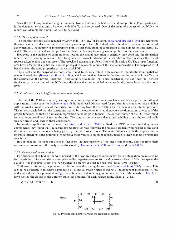
To illustrate this point, the pressure distribution over the rectangular section (H!emon and Santi, 2002) is taken. This

section has a length-to-thickness shape ratio of 2, and alternate vortex shedding is the dominant mechanism. A few

nodes over the surface presented in Fig. 1 have been selected as being good representatives of the signals. In Fig. 2, we

have plotted the clouds of the different state loci obtained for each nearest node, taken 2� 2, i.e.,

pj ¼ f ðpiÞ with j ¼ i þ 1: ð4Þ

ARTICLE IN PRESS

125497397

121

145169 193 217 241

265

289WIND

xz

125497397

121

145169 193 217 241

265

289WIND

xz

Fig. 1. Pressure taps number around the rectangular section.


One can see that the heterogeneous mean components fill the space in distinct parts, creating clusters around each

different mean value encountered. The cluster around (1, 1) is linked to the front face of the rectangle, and the cluster

around (�1, �1) to the lateral and rear sides.

In such a 2-D case, the POD method has usually a simple geometrical interpretation, since the equation

PtRP ¼ c ð5Þ

represents a set of ellipsoids centred on the origin. Then it is well known that seeking the principal components

is equivalent to seeking the principal axes of the ellipsoid, in the order of length, because ‘‘the calculations

involved in finding the principal components are precisely those necessary to find the principal axes of the

ellipsoid’’ (Marriot, 1974). This can easily be shown by developing the quadratic form (17) and searching for the ellipse

axes.

Therefore, it is obvious that the proper functions obtained by analysing the data plotted in Fig. 2 do not have a

simple physical interpretation. Moreover, extracting the mean component leads to the same results because the four

clusters will be centred on the origin and statistically mixed with each other, although their individual shape is very

different. This problem can be reinforced by the nature of the individual pressure signals when a high level of periodicity

is present.

2.2.2. Probability density function analysis

This point is in fact a major difference with some applications involving more or less random signals. In the case of

the rectangular cylinder, the harmonic component is dominant, as shown in Fig. 3 where typical samples have been

selected. The probability density functions are really different from a Gaussian shape which makes the previous

comments not completely applicable: the geometrical interpretation of the POD with ellipsoid and principal axes is

indeed restricted to multivariate normal distributions with common mean, allowing only heterogeneity of variance

(Marriot, 1974). This is probably more or less the case in the application of Tamura et al. (1999), but not at all for the

present rectangular section.

Moreover, it is obvious (in 2-D) that harmonic signals, at the same frequency, generate an ellipse in the state

plane, for which the rotation of the principal axes is directly a function of the phase angle between the two signals:

when it is zero (modulus p), the signals are perfectly correlated and the ellipse reduces to a straight line. One of the

eigenvalues is zero and the signals are linearly dependent. When the phase angle is p=2; it is possible to find the

principal axes only if the mean values have been included in the correlation matrix, because the only extra-diagonal

term consists of their product. If this term is zero, the matrix is already diagonal and the principal axes are the

original axes. Moreover, the correlation matrix obtained with non-Gaussian signals does not generally have such a

dominant diagonal as in the case of normal signals. In the limit, the principal component analysis might become

meaningless.

ARTICLE IN PRESS

−2.0 −1.5 −1.0 −0.5 0.0 0.5 1.0−2.0

−1.5

−1.0

−0.5

0.0

0.5

1.0

pi

p j

Fig. 2. State locus for 2� 2 nearest nodes around the rectangular section of Fig. 1.

P. H!emon, F. Santi / Journal of Fluids and Structures 17 (2003) 1123–1143 1127

Of course, such academic cases do not occur in practice due to the high dimension of the data set including noise: but,

nevertheless, this simple example shows the specific behaviour of harmonic signals by comparison with normally

distributed ones.

For the rectangular cylinder, the POD carried out on all the pressure distribution, including the mean value, can

deliver a physical meaning of the proper functions only by analysing also the time evolution of the principal

components, with Fourier analysis for instance. This was performed by H!emon and Santi (2002). However, it is possible

to extract the mean value of the POD, and the physical analysis needs also to be carried out on both the proper function

and the principal components. The two calculations are in fact similar, since heterogeneity of mean values always

distorts the proper functions.

In order to eliminate the distortion one may carry out the POD by parts, by analysing clusters of data having more or

less the same mean value and the same physical significance: for instance, the POD on the rectangular section could be

performed three times, one for the front side, another for the rear side, and finally for the two lateral sides. However, the

problem of cutting the clusters becomes critical for structures with more complex shapes and a general method of

decomposition is needed to ensure robustness of the technique.

ARTICLE IN PRESS

20 40 60 80 100 120−1.40

−1.20

−1.00

−0.80

−0.60

−0.40

Nod

e 28

9 (r

ear)

20 40 60 80 100 120−1.80

−1.50

−1.20

−0.90

−0.60

−0.30

Nod

e 97

(la

tera

l fro

nt)

20 40 60 80 100 120−1.80

−1.40

−1.00

−0.60

Nod

e 25

(la

tera

l rea

r)

20 40 60 80 100 1200.92

0.94

0.96

0.98

1.00

Nod

e 12

1 (f

ront

)

−1.40 −1.20 −1.00 −0.80 −0.60 −0.400

2

4

6−1.80 −1.50 −1.20 −0.90 −0.60 −0.300

1

2

3−1.80 −1.40 −1.00 −0.600

1

2

30.92 0.94 0.96 0.98 1.000

20

40

60

80

100

Reduced time Pressure coefficient

Fig. 3. Samples of pressure signals around the rectangular section. Left, pressure versus time (dimensionless); Right, corresponding

probability density function.


3. The BOD

3.1. The classical BOD

3.1.1. General presentation

The BOD has been introduced by Aubry et al. (1991) and the rigorous mathematical formulation can be found in that

paper. We present here a brief summary of the main results. The idea is to carry out a deterministic decomposition of a

space–time signal without assuming other properties of this signal beyond its square integrability. In practice, the signal

will be the result of aerodynamic measurements or computations, pressure, velocity or any other quantity, which

guarantees the above property.

The BOD of a signal Uðx; tÞ function of space xAR3 and time tAR; with Uðx; tÞAL2ðX � TÞ; XCR3 and TCR; isformally written as

Uðx; tÞ ¼XNk¼1

akckðtÞjkðxÞ: ð6Þ

The BOD theorem proves that decomposition (6) exists, converges in norm and that

a1Xa2X?X0;

limM-N

aM ¼ 0;

/jk;jlS ¼ ckcl ¼ dk;l : ð7Þ

Aubry et al. have called topos the spatial modes jkðxÞ with jkAL2ðXÞ and chronos the temporal modes ckðtÞ withckAL2ðTÞ: They proved that the topos, associated to the set of the eigenvalues a2k ¼ lk are the eigenmodes of the spatial

correlation operator

Scðx; x0Þ ¼Z

T

Uðx; tÞU � ðx0; tÞ dt; ð8Þ

which is Hermitian and nonnegative definite. The notation U� means the conjugate of U in the general case of a

complex signal. Simultaneously, the chronos associated to the same set of eigenvalues lk are the eigenmodes of the

temporal correlation operator

Tcðt; t0Þ ¼Z

X

Uðx; tÞU � ðx; t0Þ dx: ð9Þ

What is remarkable is the fact that the eigenvalues a2k are common to topos and chronos, which was proved by using

notably the symmetry property of the correlation operators. This means that chronos and topos are intrinsically

coupled because they have the same eigenvalue. However, it is possible to separate the information, spatial and

temporal, by multiplying them by the weight factorffiffiffiffiffiak

p: This remark will be useful for the application of Section 5 on

velocity field generation.

It can be shown that the continuous form of the BOD can be extended to the discrete form, in which case the

correlation operators become the correlation matrices. This assumes, however, that the observation window of the

signal is reasonably sufficient to be analysed, which means that the number of time steps and nodes is large enough.

Aubry et al. (1991) have demonstrated the robustness of the BOD when additional samples (temporal or spatial) are

taken into account in the original signal.

Another useful result in practice is the possibility to truncate decomposition (6) to M spatio-temporal structures and

that the sum of remaining terms, i.e., the truncation error, is smaller than the first neglected eigenvalue.

It has also been shown that the global energy of the signal is equal the sum of the eigenvalues

Z ZX ;T

Uðx; tÞU � ðx; tÞ dx dt ¼XNk¼1

a2k ¼ TrðScÞ ¼ TrðTcÞ: ð10Þ

The global entropy of the signal characterizing its degree of disorder is defined starting from the relative eigenvalues lrk

given by

lrk ¼ lk=XNk¼1

lk: ð11Þ


The expression of the global entropy is

H ¼ � limM-N

1

log M

XM

k¼1

lrk log lrk: ð12Þ

Due to the normalizing factor, the entropy H can be compared for different signals and it characterizes the disorder

level of the signal. When all the energy is concentrated on the first term of the decomposition, the entropy is zero. When

the energy is equally distributed among all the terms, the entropy reaches its maximum, equal to 1. In particular, the

entropy is a useful indicator when studying signals with respect to an external parameter. Aubry et al. (1991) presented

the entropy as a good way to detect the transition to turbulence for instance.

3.1.2. Links between BOD and POD

According to the developers of the BOD themselves, there is no real link between BOD and POD, since they are

based on fundamentally different principles. In fact, BOD can be seen as a time–space symmetric version of the

Karhunen–Lo"eve expansion or, in other words, a combination of the classical POD and the snapshot POD. However,

the main difference of concern for our problem is the assumptions on the analysed signal, which has to be square

integrable only for the BOD, instead of square integrable, ergodic and stationary for the POD. The BOD is a more

general method and the POD method should be considered as a particular case.

Moreover, the BOD is not derived from an optimization problem of the mean-square projection of the signal as in

POD, although the method of calculation of BOD leads also to an eigenvalue problem of a correlation operator. The

geometrical interpretation in state space, especially the principal axes of the ellipsoid vanishes in the case of BOD.

The main consequence of this concerns the discussion regarding the mean value which has to be kept in the

decomposition: there is indeed a problem in choosing among the temporal mean, the spatial mean or even the global

mean. Moreover, Aubry et al. (1991) showed that for instance in the decomposition of the temporally centred signal

Uðx; tÞ � UðxÞ ¼XNk¼1

akðckðtÞ � ckÞjkðxÞ: ð13Þ

The centred chronos ckðtÞ � ck are not orthogonal in L2ðTÞ: In this case the eigenvalues are multiplied by the factorffiffiffiffiffiffiffiffiffiffiffiffiffiffiffiffi1� ck

2q

: The remark applies similarly to a spatially centred signal. To reinforce the discussion, Aubry et al. (1991)

recall that excluding ‘‘the mean of the topos is equivalent to introducing an artificial correlation among them equal to

�/jkS/jlS for all pairs ðjk;jlÞ: Similarly, centring the chronos introduces a correlation �ckcl ’’.

3.2. Application to wall pressures

The method of BOD presented above is general and can be applied to any kind of spatio-temporal signals. In this

section the technique is adapted to wall-pressure distribution and the computation procedure is given. An extension is

then carried out in order to analyse the aerodynamic force decomposition.

In carrying out the BOD, it is first necessary to choose one kind of correlation, spatial or temporal, and to find its

eigenmodes. Secondly, the missing component, i.e., the chronos or the topos respectively, is computed with the help of

the decomposition in Eq. (6) and a suitable normalization. The calculation procedure is in fact very close to the one of

the direct POD or snapshot POD, completed by normalization. The numerical algorithm used here is the subspace

method of Bathe and Wilson but other standard eigenvalue solvers may be used.

In the standard case of pressure distribution decomposition, in relation to aerodynamic force analysis, it is obvious

that the expressions derived for the lift force by H!emon and Santi (2002) are still valid, by letting the topos equal to

the proper functions and the chronos equal to the principal components suitably normalized. However, there is the

possibility to select a priori the aerodynamic component which is involved in the study: for instance, for the rectangular

section which oscillates in a direction normal to the flow, the main interest is in the lift force.

We make the decomposition of the local lift force

CizðtÞ ¼ piðtÞAin

iz ð14Þ

where i refers to the pressure tap number and Ai is the elementary area. In what follows, the other components, drag

and pitching moment, are easily obtained by extension. When the taps are not uniformly distributed, they have not the

same weight and this should be corrected. Jeong et al. (2000) have proposed such a correction based on the weighting by

the area element of the tap, and applied to classical POD. In the present case, a correction is useless, since we just

modify the original pressure signal: the problem of area estimation and its normal vector is supposed to be solved by a

pre-processor of the BOD, depending only on the grid of pressure taps.

ARTICLE IN PRESSP. H!emon, F. Santi / Journal of Fluids and Structures 17 (2003) 1123–11431130

The terms of the spatial correlation matrix are given by

Sci;j ¼ pipjAiAjniznj

z ð15Þ

and leads satisfactorily to a symmetric matrix. However, some terms can be nullified when the wall under consideration

is parallel to the force direction which is under analysis. In practice, it will be impossible to carry out the eigenmode

calculation without restriction of the domain to nonzero terms. Aubry et al. (1991) have verified that for a restricted

domain in L2ðXÞ (or L2ðTÞ), the restricted spatial correlation operator (or temporal) preserves the BOD properties. The

elimination of the useless taps from the decomposition is possible: in practice, it has to be done in order to avoid any

numerical distortion in the eigenvalue problem resolution.

The interesting point is that the resulting force is now directly decomposed in chronos and topos since we have

CzðtÞ ¼ /CizðtÞS; assuming suitable normalization of the reference area. The BOD is now written as

CzðtÞ ¼XM

k¼1Czk

ðtÞ ¼XM

k¼1akckðtÞ/jkS: ð16Þ

It can be shown that the properties of orthogonality are preserved for the quadratic mean values and lead to an

indicator of convergence of the decomposition, in terms of force

Ezk¼ Czk

ðtÞ2=CzðtÞ2; ð17Þ

which is usually given as a percentage. An entropy, specifically dedicated to the lift force, can then be defined by analogy

Hz ¼ �1

log M

XM

k¼1Ezk

log Ezk: ð18Þ

In order to illustrate the application of these tools, we present in the following section two examples on classical bluff

body flows. It should be noted before that the simultaneous analysis of two components, for instance X and Z; ismathematically possible although it has no sense from a mechanical point of view, the two components being already

orthogonal in the physical space. In this case, the phase difference between the two fluctuating forces is fixed by the

chronos of each component independently.

4. Application of the BOD on pressure distributions

4.1. Rectangular prism

This case was presented in detail by H!emon and Santi (2002) and we recall here the main points. The pressure data

are the results from the computations with a Navier–Stokes solver. It solves the 2-D incompressible unsteady equations

without turbulence modelling. The section of the rectangle has a length-to-thickness ratio of 2, and the Reynolds

number is 6000 based on the length. Grid refinement was chosen so as to capture correctly the physics of the large

coherent structures.

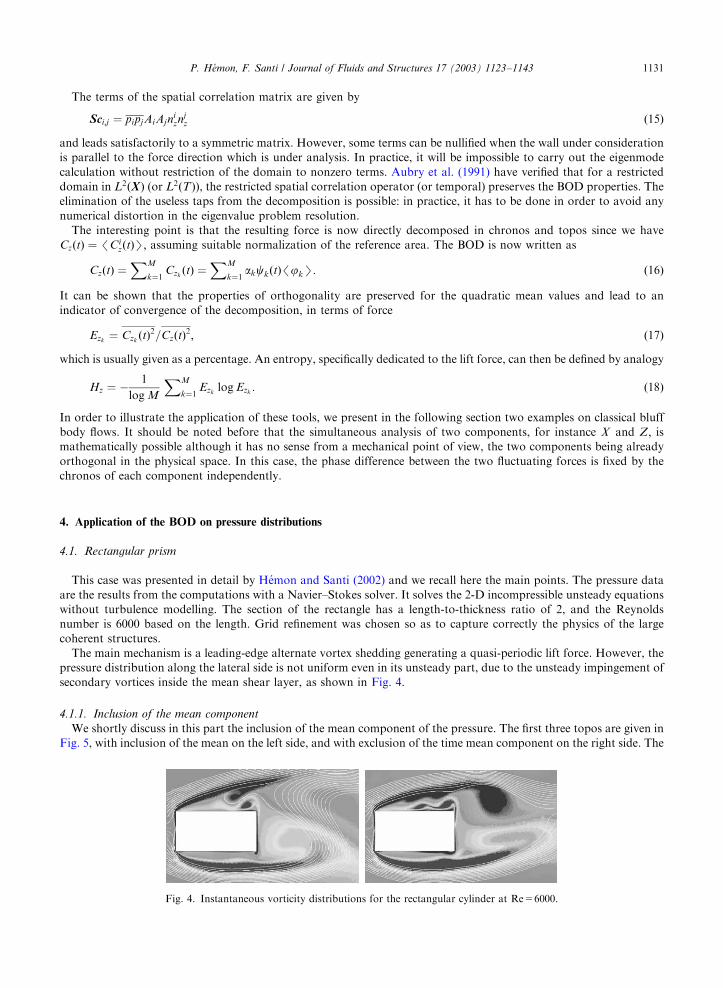
The main mechanism is a leading-edge alternate vortex shedding generating a quasi-periodic lift force. However, the

pressure distribution along the lateral side is not uniform even in its unsteady part, due to the unsteady impingement of

secondary vortices inside the mean shear layer, as shown in Fig. 4.

4.1.1. Inclusion of the mean component

We shortly discuss in this part the inclusion of the mean component of the pressure. The first three topos are given in

Fig. 5, with inclusion of the mean on the left side, and with exclusion of the time mean component on the right side. The

ARTICLE IN PRESS

Fig. 4. Instantaneous vorticity distributions for the rectangular cylinder at Re=6000.


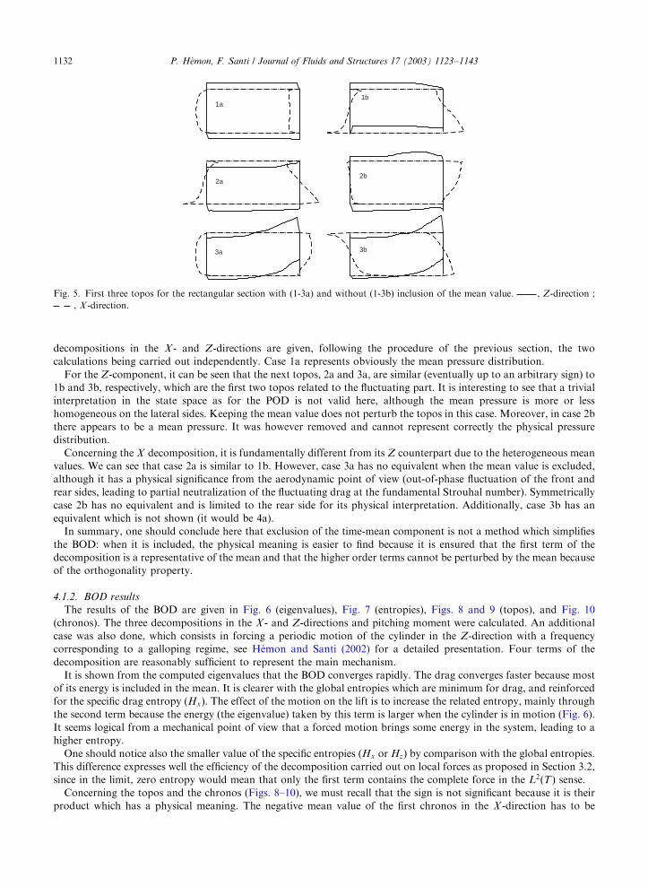
decompositions in the X - and Z-directions are given, following the procedure of the previous section, the two

calculations being carried out independently. Case 1a represents obviously the mean pressure distribution.

For the Z-component, it can be seen that the next topos, 2a and 3a, are similar (eventually up to an arbitrary sign) to

1b and 3b, respectively, which are the first two topos related to the fluctuating part. It is interesting to see that a trivial

interpretation in the state space as for the POD is not valid here, although the mean pressure is more or less

homogeneous on the lateral sides. Keeping the mean value does not perturb the topos in this case. Moreover, in case 2b

there appears to be a mean pressure. It was however removed and cannot represent correctly the physical pressure

distribution.

Concerning the X decomposition, it is fundamentally different from its Z counterpart due to the heterogeneous mean

values. We can see that case 2a is similar to 1b. However, case 3a has no equivalent when the mean value is excluded,

although it has a physical significance from the aerodynamic point of view (out-of-phase fluctuation of the front and

rear sides, leading to partial neutralization of the fluctuating drag at the fundamental Strouhal number). Symmetrically

case 2b has no equivalent and is limited to the rear side for its physical interpretation. Additionally, case 3b has an

equivalent which is not shown (it would be 4a).

In summary, one should conclude here that exclusion of the time-mean component is not a method which simplifies

the BOD: when it is included, the physical meaning is easier to find because it is ensured that the first term of the

decomposition is a representative of the mean and that the higher order terms cannot be perturbed by the mean because

of the orthogonality property.

4.1.2. BOD results

The results of the BOD are given in Fig. 6 (eigenvalues), Fig. 7 (entropies), Figs. 8 and 9 (topos), and Fig. 10

(chronos). The three decompositions in the X - and Z-directions and pitching moment were calculated. An additional

case was also done, which consists in forcing a periodic motion of the cylinder in the Z-direction with a frequency

corresponding to a galloping regime, see H!emon and Santi (2002) for a detailed presentation. Four terms of the

decomposition are reasonably sufficient to represent the main mechanism.

It is shown from the computed eigenvalues that the BOD converges rapidly. The drag converges faster because most

of its energy is included in the mean. It is clearer with the global entropies which are minimum for drag, and reinforced

for the specific drag entropy (Hx). The effect of the motion on the lift is to increase the related entropy, mainly through

the second term because the energy (the eigenvalue) taken by this term is larger when the cylinder is in motion (Fig. 6).

It seems logical from a mechanical point of view that a forced motion brings some energy in the system, leading to a

higher entropy.

One should notice also the smaller value of the specific entropies (Hx or Hz) by comparison with the global entropies.

This difference expresses well the efficiency of the decomposition carried out on local forces as proposed in Section 3.2,

since in the limit, zero entropy would mean that only the first term contains the complete force in the L2ðTÞ sense.Concerning the topos and the chronos (Figs. 8–10), we must recall that the sign is not significant because it is their

product which has a physical meaning. The negative mean value of the first chronos in the X -direction has to be

ARTICLE IN PRESS

1a

2a

3a

1b

2b

3b

Fig. 5. First three topos for the rectangular section with (1-3a) and without (1-3b) inclusion of the mean value. , Z-direction ;

, X -direction.


multiplied by its negative counterpart in the corresponding topos, thereby keeping the product positive as one would

expect for the mean drag coefficient.

The analysis of the Z-component is more significant in this problem. We observe that the second term of the BOD is

the fluctuating force generated by the leading-edge vortex shedding embracing all the lateral sides. The third term,

which creates the main part of the fluctuating pitching moment, is concerned with the periodic impinging of the main

leading-edge vortices. At a smaller scale, the fourth term is the first one related to the secondary vortices inside the shear

layer: this weaker mechanism requires however higher terms to be correctly described.

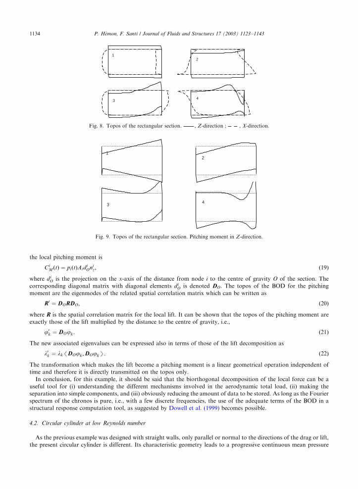
The analysis of the pitching moment with respect to the centre of the cylinder was carried out using only the local

forces in the Z-direction, the contribution of the local drag forces being neglected. The topos are shown in Fig. 9, and

the chronos were found similar to those of the lift force. It is interesting to notice that the topos are in fact exactly

similar also, the difference being due to the product of the local lift by the distance to the centre of the cylinder. Indeed,

ARTICLE IN PRESS

1 2 3 4 5 6Mode number

10−3

10−2

10−1

100

101

102

Eig

enva

lue

(%)

Fig. 6. Eigenvalues for the rectangular section: J, X -direction ; n, Z-direction ; m, Z-direction in forced oscillations.

1 2 3 4 5 6Mode number

0.0

1.0

2.0

3.0

5

10

15

20

25

H(%

)H

xor

Hz

(%)

Fig. 7. Cumulated entropy for the rectangular section: J, X -direction ; n, Z-direction ; m, Z-direction in forced oscillations.


the local pitching moment is

CiM ðtÞ ¼ piðtÞAid

iOni

z; ð19Þ

where diO is the projection on the x-axis of the distance from node i to the centre of gravity O of the section. The

corresponding diagonal matrix with diagonal elements diO is denoted DO: The topos of the BOD for the pitching

moment are the eigenmodes of the related spatial correlation matrix which can be written as

R0 ¼ DORDO; ð20Þ

where R is the spatial correlation matrix for the local lift. It can be shown that the topos of the pitching moment are

exactly those of the lift multiplied by the distance to the centre of gravity, i.e.,

j0k ¼ DOjk: ð21Þ

The new associated eigenvalues can be expressed also in terms of those of the lift decomposition as

l0k ¼ lk/DOjk;DOjkS: ð22Þ

The transformation which makes the lift become a pitching moment is a linear geometrical operation independent of

time and therefore it is directly transmitted on the topos only.

In conclusion, for this example, it should be said that the biorthogonal decomposition of the local force can be a

useful tool for (i) understanding the different mechanisms involved in the aerodynamic total load, (ii) making the

separation into simple components, and (iii) obviously reducing the amount of data to be stored. As long as the Fourier

spectrum of the chronos is pure, i.e., with a few discrete frequencies, the use of the adequate terms of the BOD in a

structural response computation tool, as suggested by Dowell et al. (1999) becomes possible.

4.2. Circular cylinder at low Reynolds number

As the previous example was designed with straight walls, only parallel or normal to the directions of the drag or lift,

the present circular cylinder is different. Its characteristic geometry leads to a progressive continuous mean pressure

ARTICLE IN PRESS

12

3 4

Fig. 8. Topos of the rectangular section. , Z-direction ; , X-direction.

12

3 4

Fig. 9. Topos of the rectangular section. Pitching moment in Z-direction.


distribution which does not create well-formed clusters of data in state space as for the rectangle. This illustration case is

therefore complementary to the previous one.

The 2-D circular cylinder is one of the most documented cases of bluff body flow due to the alternate vortex street

generated for a given range of Reynolds numbers. The purpose of this section is limited to the illustration of the BOD

method: the pressure data are obtained through a numerical simulation of the flow using the same Navier–Stokes solver

as for the rectangular section. The simulated equivalent Reynolds number is 150, leading to a well-established alternate

vortex regime. The data set consists of 100 nodes with 950 time steps, representing 19 periods of the alternate shedding.

Three kinds of BOD have been calculated, with the pressure distribution (scalar) and with the local forces in the

longitudinal (X ) and lateral (Z) directions.

The cumulated entropies are given in Fig. 11. For the BOD on the pressure, the specific entropies obtained by

recombination of drag and lift are given also: they are not equivalent to those obtained by decomposition of local

ARTICLE IN PRESS

40 50 60 70 80 90 100 110Reduced time

−0.050.000.05

−0.050.000.05

−0.050.000.05

−0.050.000.05

40 50 60 70 80 90 100 110Reduced time

−0.050.000.05

−0.050.000.05

−0.050.000.05

−0.050.000.05

Fig. 10. Chronos of the rectangular section. Left, X -direction; Right, Z-direction.

1 2 3 4 5Mode number

10−2

10−1

100

101

2

4

6

8

10

Hx

orH

z(%

)H

(%)

Fig. 11. Cumulated entropy for the circular cylinder. Filled symbols, pressure analysis; Open symbols, local force analysis ; J, K, X -

direction ; n, m, Z-direction.


forces. The specific entropies show the large difference between the X - and Z-directions: the method based on the X - or

Z decomposition of the local force is seen to be much sensitive to the selected direction than the corresponding

decomposition of the pressure. This demonstrates objectively that the spatio-temporal complexity is much larger for the

lift component (two orders of magnitude) than for the drag component. One must recall however that this criterion is

based on mean-square values.

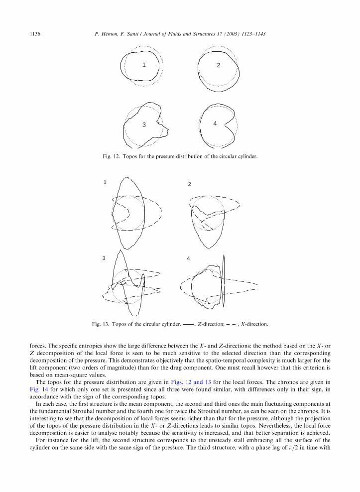
The topos for the pressure distribution are given in Figs. 12 and 13 for the local forces. The chronos are given in

Fig. 14 for which only one set is presented since all three were found similar, with differences only in their sign, in

accordance with the sign of the corresponding topos.

In each case, the first structure is the mean component, the second and third ones the main fluctuating components at

the fundamental Strouhal number and the fourth one for twice the Strouhal number, as can be seen on the chronos. It is

interesting to see that the decomposition of local forces seems richer than that for the pressure, although the projection

of the topos of the pressure distribution in the X - or Z-directions leads to similar topos. Nevertheless, the local force

decomposition is easier to analyse notably because the sensitivity is increased, and that better separation is achieved.

For instance for the lift, the second structure corresponds to the unsteady stall embracing all the surface of the

cylinder on the same side with the same sign of the pressure. The third structure, with a phase lag of p=2 in time with

ARTICLE IN PRESS

1 2

3 4

Fig. 12. Topos for the pressure distribution of the circular cylinder.

1 2

3 4

Fig. 13. Topos of the circular cylinder. , Z-direction; , X -direction.


respect to the second, corresponds to a local force distribution which expresses the out-of-phase behaviour between the

front and rear part of one side of the cylinder.

Considering only structures 2 and 3, one could object here that the orthogonality requirements should obviously lead

to such topos and chronos. This has to be tempered (i) by the fact that the physics can lead here to such results because

the signals are relatively close to being harmonic, and (ii) by the small eigenvalue affected in the third structure which

makes it not so important in amplitude.

In summary, this simple example confirms the previous conclusions obtained with the rectangular cylinder and adds a

complementary remark concerning the separation a priori of the force components, or a posteriori by recombination

with the BOD of the pressure: in such a simple case, the geometry does not lead to clusters in state space, and separation

of components a priori is not so efficient. This is reinforced by the fact that the chronos were found identical in the three

BOD. Nevertheless, for complex structures, involving sharp angles for instance, the spatial complexity is such that the

separation a priori of the components will lead to better efficiency of the decomposition.

5. Simulation of a spatially correlated velocity field

We present in this section an application of the BOD to the modelling of a velocity field. The purpose is very different

from the previous sections where the BOD was used as an analysis tool for already available signals: the objective here is

to generate the signal by using the specific properties of the BOD.

In the field of wind-excited structures, temporal simulations are increasingly important, due to the large size of the

structures as, for instance, in modern suspended bridges (AFGC, 2002). As a consequence, there is a need for more

accurate computations which can include the nonlinear behaviour of the structure. However, the classical techniques

for solving the dynamical problem are generally based on spectral methods in which the nonlinear part, structural and

even aeroelastic, is difficult to introduce.

The temporal simulation of the aeroelastic coupled problem, including atmospheric turbulence excitation, requires

considerable input data in terms of a velocity field: this field has to be close to the real turbulent wind, one essential

characteristic of which is the spatial correlation. There exist a number of methods for generating a turbulent velocity

field as presented in the review by Guillin and Cr!emona (1997) and Di Paola (1998).

One of them is derived from the method proposed by Yamazaki and Shinozuka (1990) for application in earthquake

engineering. Their approach which is called statistical preconditioning, is based on the modal decomposition of the

spatial covariance matrix and the temporal part of the signal is generated by using a Fourier decomposition. Recently,

Carassale and Solari (2002) similarly used the direct POD to generate a turbulent wind velocity field and to compute the

wind loads acting on the eigenmodes of a structure.

ARTICLE IN PRESS

75 100 125 150 175 200Reduced time

−0.050.000.05

−0.050.000.05

−0.050.000.05

−0.050.000.05

Fig. 14. Chronos of the circular cylinder.


The method can be improved by exploiting the space-time symmetry of the BOD, as outlined below. We emphasize

that our objective is to illustrate the use of the BOD technique. We will not enter into the details of the physical

modelling of the wind: more information can be found in the related literature, as in AFGC (2002) and references

therein.

5.1. Initial data

In the civil engineering community, the turbulent wind is usually described by a few statistical parameters which

constitute the targets for the simulated wind field. We derive in this section the expressions related to the vertical

velocity component w of the turbulence which is applied to an elongated horizontal structure, such as a bridge deck.

The formulation can readily be extended to the other components.

The target parameters describing the atmospheric turbulent wind are (i) the horizontal mean velocity %UðzÞ; which maybe a function of the altitude z; (ii) the standard deviation of the vertical velocity sw; (iii) the power spectral density(PSD) of the vertical velocity Swðf Þ versus frequency f ; and (iv) the coherence function of the vertical velocity in the

lateral direction gywðf Þ:

The PSD function and the coherence function may come from different sources and we have chosen here the most

common modelling, i.e., the von K!arm!an spectrum

Swðf Þs2w

¼4Lx

w

%UðzÞ1þ 188:4 2fLx

w= %UðzÞ� 2

1þ 70:7 2fLxw= %UðzÞ

� 2 �11=6 ð23Þ

and an exponential coherence function between points i and j given by

gi;jw ðf Þ ¼ exp

�Cywjyi � yj jf%UðzÞ

� ; ð24Þ

where Lxw is the longitudinal scale of the vertical velocity component and Cy

w the coherence coefficient of the vertical

velocity in the lateral y direction. It should be noted that the PSD is normalized by definition with the square of the

standard deviation.

All the parameters appearing in the target characteristics are usually extracted from literature data or from in situ

measurements and meteorological studies, especially when the site effect can be significant, as for instance in a

mountainous area.

It should be noted that a complete 2-D field cannot be built due to the lack of modelling for the cross-spectral density

function; for instance, for a horizontal and vertical structure, such as a suspended bridge including the deck and the

pylons, the cross-spectrum between lateral and vertical turbulence is needed. Unfortunately, there is actually no

generally accepted modelling. Therefore, we give in the following a single-component application that may be extended

to two components, provided the cross-spectrum is known.

5.2. Development of the method with BOD

The idea is to generate a wind velocity field which is given by a BOD as

Uðy; tÞ ¼XM

m¼1

ffiffiffiffiffiffiat

m

pcmðtÞ

ffiffiffiffiffiffiay

m

pjmðyÞ; ð25Þ

where the chronos are associated with the set of eigenvalues ðatmÞ

2 and the topos with ðaymÞ

2: The main point is to find thetopos and the chronos separately by solving twice the corresponding eigenvalue problem.

By assuming a suitable discretization in time and space, which will be discussed below, the spatial correlation matrix

is built starting from the spectral density functions between nodes i and j as

Sci;j ¼X

l

ffiffiffiffiffiffiffiffiffiffiffiffiffiffiffiffiffiffiffiffiffiffiffiffiffiffiSwi

ðflÞSwjðflÞ

qgi;j

w ðflÞ; ð26Þ

where the index l refers to the frequency. The integration over the frequency band has to be compatible with the time

discretization.

For the chronos, we assume that the individual signals at point i and time tk are built with Fourier series as

wiðtkÞ ¼X

l

ffiffiffiffiffiffiffiffiffiffiffiffiffiffiffi2Swi

ðflÞp

cos ð2pfl tk þ fi;lÞ; ð27Þ

where the phase angles fi;l are randomly uniformly distributed in ½0; 2p�: The temporal correlation matrix is given by

Tck;n ¼X

twiðtkÞwiðtnÞ: ð28Þ

ARTICLE IN PRESSP. H!emon, F. Santi / Journal of Fluids and Structures 17 (2003) 1123–11431138

From the definitions given above, it can be shown that the total energy of the signal given by the trace of each

correlation matrix is

TrðTcÞ ¼ Ks2w; TrðScÞ ¼ Ns2w; ð29Þ

where K and N are the number of time steps and the number of nodes, respectively. It becomes therefore obvious that

these numbers have to be equal, a constraint which did not appear clearly in the previous section. The time–space

symmetry of the BOD was not really employed for the analysis of existing available signals, and the dimensions of each

set, temporal or spatial, were implicitly assumed to be equal. In the present case, the explicit equality is necessary and

the following application will illustrate the constraints that result from this equality.

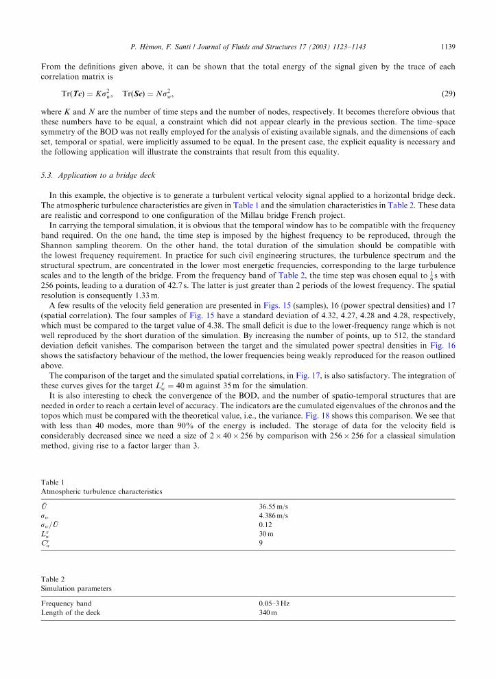
5.3. Application to a bridge deck

In this example, the objective is to generate a turbulent vertical velocity signal applied to a horizontal bridge deck.

The atmospheric turbulence characteristics are given in Table 1 and the simulation characteristics in Table 2. These data

are realistic and correspond to one configuration of the Millau bridge French project.

In carrying the temporal simulation, it is obvious that the temporal window has to be compatible with the frequency

band required. On the one hand, the time step is imposed by the highest frequency to be reproduced, through the

Shannon sampling theorem. On the other hand, the total duration of the simulation should be compatible with

the lowest frequency requirement. In practice for such civil engineering structures, the turbulence spectrum and the

structural spectrum, are concentrated in the lower most energetic frequencies, corresponding to the large turbulence

scales and to the length of the bridge. From the frequency band of Table 2, the time step was chosen equal to 16s with

256 points, leading to a duration of 42.7 s. The latter is just greater than 2 periods of the lowest frequency. The spatial

resolution is consequently 1.33m.

A few results of the velocity field generation are presented in Figs. 15 (samples), 16 (power spectral densities) and 17

(spatial correlation). The four samples of Fig. 15 have a standard deviation of 4.32, 4.27, 4.28 and 4.28, respectively,

which must be compared to the target value of 4.38. The small deficit is due to the lower-frequency range which is not

well reproduced by the short duration of the simulation. By increasing the number of points, up to 512, the standard

deviation deficit vanishes. The comparison between the target and the simulated power spectral densities in Fig. 16

shows the satisfactory behaviour of the method, the lower frequencies being weakly reproduced for the reason outlined

above.

The comparison of the target and the simulated spatial correlations, in Fig. 17, is also satisfactory. The integration of

these curves gives for the target Lyw ¼ 40 m against 35m for the simulation.

It is also interesting to check the convergence of the BOD, and the number of spatio-temporal structures that are

needed in order to reach a certain level of accuracy. The indicators are the cumulated eigenvalues of the chronos and the

topos which must be compared with the theoretical value, i.e., the variance. Fig. 18 shows this comparison. We see that

with less than 40 modes, more than 90% of the energy is included. The storage of data for the velocity field is

considerably decreased since we need a size of 2� 40� 256 by comparison with 256� 256 for a classical simulation

method, giving rise to a factor larger than 3.

ARTICLE IN PRESS

Table 1

Atmospheric turbulence characteristics

%U 36.55m/s

sw 4.386m/s

sw= %U 0.12

Lxw 30m

Cyw 9

Table 2

Simulation parameters

Frequency band 0.05–3Hz

Length of the deck 340m


It should be said also, from a physical point of view, that the higher frequencies are spatially less correlated, which is

a characteristic of the turbulence. Due to this, the convergence of the BOD is always better in the low-frequency range.

The last remark concerns the signal construction by Eq. (25), with the help of topos and chronos that are computed

independently. This is the central point of the technique. It implies that for a given chronos, the associated topos (i.e., of

same order) is fixed and reciprocally. This assumption is not ensured a priori and should require further mathematical

investigations. The results show however that the behaviour is very satisfactory because the two sets of eigenvalues

(topos and chronos) have a very close convergence evolution, as seen in Fig. 18.

Another point is the determinism of the method, although there is apparently a stochastic part in Eq. (27) for the

chronos estimation. Complete determinism is obtained through the truncation of the decomposition by retaining the

first M chronos and topos. We give in Fig. 19 the first four chronos and topos. We see that the topos have a wavelength

which decreases as their order increases. Consequently, the associated chronos have a main frequency which increases

simultaneously. It is consistent with the mechanical point of view and explains the good behaviour of the decomposition

given by Eq. (25).

In conclusion, it should be said that the BOD is a very convenient, even elegant, technique for generating

spatially correlated fields, such as atmospheric wind. It can be used also for earthquake engineering. Moreover, the

ARTICLE IN PRESS

0 10 20 30 40

−10

0

10

(m/s

)

−10

0

10(m

/s)

−10

0

10

(m/s

)

−10

0

10

(m/s

)

Time (s)

Fig. 15. Samples of generated time histories of wðtÞ:

0.1 1.0

Frequency (Hz)

10−4

10−3

10−2

10−1

100

S w

Fig. 16. Comparison of power spectral densities. , target function ; , samples of Fig. 15.


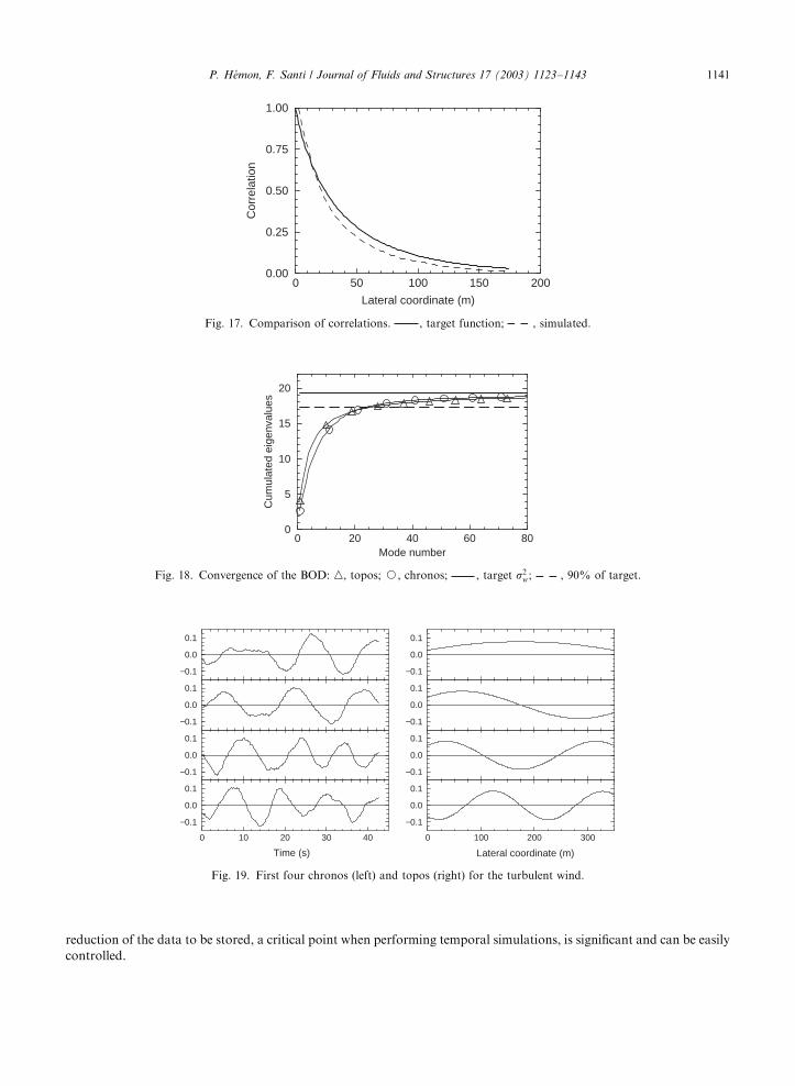
reduction of the data to be stored, a critical point when performing temporal simulations, is significant and can be easily

controlled.

ARTICLE IN PRESS

0 50 100 150 200

Lateral coordinate (m)

0.00

0.25

0.50

0.75

1.00

Cor

rela

tion

Fig. 17. Comparison of correlations. , target function; , simulated.

0 20 40 60 80Mode number

0

5

10

15

20

Cum

ulat

ed e

igen

valu

es

Fig. 18. Convergence of the BOD: n, topos; J, chronos; , target s2w; , 90% of target.

0 10 20 30 40

−0.1

0.0

0.1

−0.1

0.0

0.1

−0.1

0.0

0.1

−0.1

0.0

0.1

0 100 200 300

−0.1

0.0

0.1

−0.1

0.0

0.1

−0.1

0.0

0.1

−0.1

0.0

0.1

Time (s) Lateral coordinate (m)

Fig. 19. First four chronos (left) and topos (right) for the turbulent wind.


6. Conclusion and further applications

We have presented the biorthogonal decomposition of spatio-temporal signals proposed by Aubry et al. (1991) in the

context of fluid–structure interaction problems. This tool generalizes the so-called POD in the sense that the signal is

not necessarily ergodic and stationary. In most cases, the biorthogonal decomposition should replace the classical POD

and it should be applicable to a wider variety of situations.

For instance, we have adapted the method to the analysis of the wall-pressure distribution and discussed the problem

of the inclusion of the mean values, especially when heterogeneities are present. In such a case, we have shown that the

POD is submitted to distortions because it is employed arbitrarily with signals which do not satisfy the fundamental

assumptions.

We have also proposed to use the BOD in order to generate a turbulent velocity field: the method is based on the

space-time symmetry of the BOD which is imperative for this application and not possible with POD. A test-case was

presented and shows that the reduction of the amount of stored data is considerable by comparison with other methods

based, for instance, on Fourier transform.

Various extensions can be done on the decomposed signals, for instance if the data are available, the decomposition

onto local flutter derivatives could be performed, so that the different coherent structures detected could be associated

to a specific structural action, such as aerodynamic damping. Amandol"ese (2001) has partially initiated the process with

POD. By using BOD instead, the specific entropy would be a very sensitive indicator in aeroelastic stability by reference

to a control parameter such as the reduced velocity.

Still in the fluid–structure interactions domain, the BOD can be seen as a powerful method of filtering

experimental data in order to make them more comprehensive and ready for suitable processing. A simple example is

given by the problem of vortex-induced waves along cables currently studied at LadHyX (Facchinetti et al., 2002).

In this application, a long flexible cable is submitted to vortex-shedding excitation and the question is to detect

the presence of travelling waves rather than standing ones. The experiments are carried out in a water tank at low

Reynolds numbers, of the order of 100. The measurement technique involves a numerical video camera, which

provides a numerical movie. After processing, the lateral displacement of a given length of the cable is obtained versus

time.

The BOD is carried out on this signal where the space dimension is reduced to a single vertical coordinate. The results

show that only the first two terms are sufficient to recover correctly the original signal at 90% in energy, the first term

having roughly an eigenvalue twice the second. The topos and chronos are given in Fig. 20. The main frequency visible

on the chronos allows to recover the Strouhal number. From these results, it is possible to demonstrate objectively the

presence of travelling waves and also to quantify the incident and reflexive part by a quantitative use of the eigenvalues

and of the phase lag between the chronos.

ARTICLE IN PRESS

0 1 2 3 4 5 6−0.20

−0.10

0.00

0.10

0.20

−0.15 0 0.15−75

−25

25

75

125

Chr

onos

Ver

tical

coo

rdin

ate

(mm

)

ToposTime (s)

Fig. 20. First two chronos and topos of a vortex-excited cable: , first; , second.


References

AFGC, 2002. In: Cr!emona, C., Foucriat, J.-C., (Eds.), Comportement au vent des ponts. Presses de l’Ecole Nationale des Ponts et

Chauss!ees, Paris.

Amandol"ese, X., 2001. Contribution "a l’!etude des chargements fluides sur des obstacles non profil!es fixes ou mobiles. Ph.D. Thesis,

Ecole Nationale des Ponts et Chauss!ees, Paris, France.

Armitt, J., 1968. Eigenvector analysis of pressure fluctuations on the West Burton instrumented cooling tower. Internal Report

RD/L/N 114/68, Central Electricity Research Laboratories (UK), unpublished.

Arndt, R.E.A., Long, D.F., Glauser, M.N., 1997. The proper orthogonal decomposition of pressure fluctuations surrounding a

turbulent jet. Journal of Fluid Mechanics 340, 1–33.

Aubry, N., Guyonnet, R., Lima, R., 1991. Spatiotemporal analysis of complex signals: theory and applications. Journal of Statistical

Physics 64, 683–739.

Breuer, K.S., Sirovich, L., 1991. The use of Karhunen-Lo!eve procedure for the calculation of linear eigenfunctions. Journal of

Computational Physics 96, 277–296.

Carassale, L., Solari, G., 2002. Wind modes for structural dynamics: a continuous approach. Probabilistic Engineering Mechanics 17,

157–166.

Cordier, L., 1996. Etude de syst"emes dynamiques bas!es sur la decomposition orthogonale aux valeurs propres. Application "a la couche

de m!elange turbulente et "a l’!ecoulement entre deux disques contra-rotatifs. Ph. D. Thesis, Universit!e de Poitiers, Poitiers, France.

Delville, J., Ukeiley, L., Cordier, L., Bonnet, J.P., Glauser, M., 1999. Examination of large scale structures in a turbulent plane mixing

layer. Part 1. Proper orthogonal decomposition. Journal of Fluid Mechanics 391, 91–122.

Di Paola, M., 1998. Digital simulation of wind field velocity. Journal of Wind Engineering and Industrial Aerodynamics 74–76,

91–109.

Dowell, E.H., Hall, C., Thomas, J.P., Florea, R., Epureanu, B.I., Heeg, J., 1999. Reduced order models in unsteady aerodynamics.

Proceedings of Third International Conference on Aero-Hydroelasticity, Vol. 3, Prague, August 30–September, pp. 20–35.

Facchinetti, M., de Langre, E., Biolley, F., 2002. Vortex-induced waves along cables. ASME Paper IMECE2002-32161, Fifth

symposium on FSI, AE & FIV+N, November 17–22, New Orleans, USA.

Feeny, B.F., Kappagantu, R., 1998. On the physical interpretation of proper orthogonal modes in vibrations. Journal of Sound and

Vibration 211, 607–616.

Guillin, A., Cr!emona, C., 1997. D!eveloppement d’algorithmes de simulation de champs de vitesse de vent. Report of Laboratoire

Central des Ponts et Chauss!ees, section Ouvrages d’Art, OA27, Paris, France.

H!emon, P., Santi, F., 2002. On the aeroelastic behaviour of rectangular cylinders in cross-flow. Journal of Fluids and Structures 16,

855–889.

Holmes, P., Lumley, J.L., Berkooz, G., 1996. Turbulence, Coherent Structures and Symmetry. Cambridge University Press,

Cambridge.

Holmes, J.D., Sankaran, R., Kwok, K.C.S., Syme, M.J., 1997. Eigenvector mode of fluctuating pressures on low-rise building models.

Journal of Wind Engineering and Industrial Aerodynamics 69–71, 697–707.

Jeong, S.H., Bienkiewicz, B., Ham, H.J., 2000. Proper orthogonal decomposition of building wind pressure specified at non-uniformly

distributed pressure taps. Journal of Wind Engineering and Industrial Aerodynamics 87, 1–14.

Lebart, L., Morineau, A., Fenelon, J.-P., 1982. Traitement des donn!ees statistique. 2"eme !edition. Dunod, Paris.

Letchford, C.W., Sarkar, P.P., 2000. Mean and fluctuating wind loads on rough and smooth parabolic domes. Journal of Wind

Engineering and Industrial Aerodynamics 88, 101–117.

Marriott, F.H.C., 1974. The Interpretation of Multiple Observations. Academic Press, London.

Tamura, Y., Suganuma, S., Kikuchi, H., Hibi, K., 1999. Proper orthogonal decomposition of random wind pressure field. Journal of

Fluids and Structures 13, 1069–1095.

Yamazaki, F., Shinozuka, M., 1990. Simulation of stochastic fields by statistical preconditioning. ASCE Journal of Engineering

Mechanics 116, 268–287.


applicationsofbiorthogonaldecompositionsin ﬂuid ... a,*,f.santib ahydrodynamics laboratory,...

Documents