applied math 205 -...
TRANSCRIPT

Applied Math 205
I Full office hour schedule:I Yue: Monday 5pm–6:30pm, IACS lounge1
I Nick: Tuesday 9am–10:30am, IACS loungeI Chris: Tuesday 1pm–3pm, Pierce Hall, Room 305I Dan: Thursday 2:30pm–4:30pm, IACS lounge
1If you are in the Maxwell–Dworkin lobby facing the lecture hall, then theIACS lounge is off to the left.

Bernstein interpolation
The Bernstein polynomials on [0, 1] are
bm,n(x) =
(nm
)xm(1− x)n−m.
For a function f on the [0, 1], the approximating polynomial is
Bn(f )(x) =n∑
m=0
f(mn
)bm,n(x).
Bernstein interpolation is impractical for normal use, and convergesextremely slowly. However, it has robust convergence properties,which can be used to prove the Weierstraß approximation theorem.See a textbook on real analysis for a full discussion.2
2e.g. Elementary Analysis by Kenneth A. Ross

Bernstein interpolation
-1
-0.5
0
0.5
1
0 0.2 0.4 0.6 0.8 1
x
Bernstein polynomialsf(x)

Bernstein interpolation
-0.2
-0.1
0
0.1
0.2
0.3
0.4
0.5
0.6
0.7
0 0.2 0.4 0.6 0.8 1
x
Bernstein polynomialsg(x)

Lebesgue Constant
Then, we can relate interpolation error to ‖f − p∗n‖∞ as follows:
‖f − In(f )‖∞ ≤ ‖f − p∗n‖∞ + ‖p∗n − In(f )‖∞= ‖f − p∗n‖∞ + ‖In(p∗n)− In(f )‖∞= ‖f − p∗n‖∞ + ‖In(p∗n − f )‖∞
= ‖f − p∗n‖∞ +‖In(p∗n − f )‖∞‖p∗n − f ‖∞
‖f − p∗n‖∞
≤ ‖f − p∗n‖∞ + Λn(X )‖f − p∗n‖∞= (1 + Λn(X ))‖f − p∗n‖∞

Lebesgue Constant
Small Lebesgue constant means that our interpolation can’t bemuch worse that the best possible polynomial approximation!
[lsum.py ] Now let’s compare Lebesgue constants for equispaced(Xequi) and Chebyshev points (Xcheb)

Lebesgue Constant
Plot of∑10
k=0 |Lk(x)| for Xequi and Xcheb (11 pts in [−1, 1])
−1 −0.5 0 0.5 10
5
10
15
20
25
30
−1 −0.5 0 0.5 11
1.5
2
2.5
Λ10(Xequi) ≈ 29.9 Λ10(Xcheb) ≈ 2.49
Lebesgue Constant
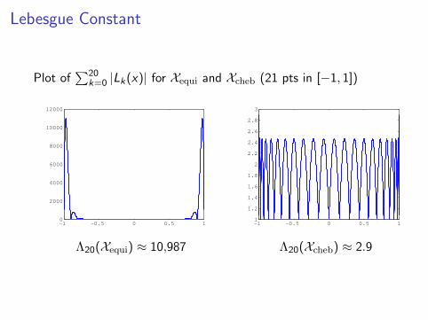
Plot of∑20
k=0 |Lk(x)| for Xequi and Xcheb (21 pts in [−1, 1])
−1 −0.5 0 0.5 10
2000
4000
6000
8000
10000
12000
−1 −0.5 0 0.5 11
1.2
1.4
1.6
1.8
2
2.2
2.4
2.6
2.8
3
Λ20(Xequi) ≈ 10,987 Λ20(Xcheb) ≈ 2.9

Lebesgue Constant
Plot of∑30
k=0 |Lk(x)| for Xequi and Xcheb (31 pts in [−1, 1])
−1 −0.5 0 0.5 10
1
2
3
4
5
6
7x 10
6
−1 −0.5 0 0.5 11
1.5
2
2.5
3
3.5
Λ30(Xequi) ≈ 6,600,000 Λ30(Xcheb) ≈ 3.15
Lebesgue Constant
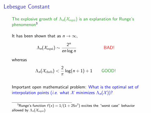
The explosive growth of Λn(Xequi) is an explanation for Runge’sphenomenon3
It has been shown that as n→∞,
Λn(Xequi) ∼2n
en log nBAD!
whereas
Λn(Xcheb) <2
πlog(n + 1) + 1 GOOD!
Important open mathematical problem: What is the optimal set ofinterpolation points (i.e. what X minimizes Λn(X ))?
3Runge’s function f (x) = 1/(1 + 25x2) excites the “worst case” behaviorallowed by Λn(Xequi)

Summary
It is helpful to compare and contrast the two key topics we’veconsidered so far in this chapter
1. Polynomial interpolation for fitting discrete data:
I We get “zero error” regardless of the interpolation points, i.e.we’re guaranteed to fit the discrete data
I Should use Lagrange polynomial basis (diagonal system,well-conditioned)
2. Polynomial interpolation for approximating continuousfunctions:
I For a given set of interpolating points, uses the methodologyfrom 1 above to construct the interpolant
I But now interpolation points play a crucial role in determiningthe magnitude of the error ‖f − In(f )‖∞

Piecewise Polynomial Interpolation

Piecewise Polynomial Interpolation
We can’t always choose our interpolation points to be Chebyshev,so another way to avoid “blow up” is via piecewise polynomials
Idea is simple: Break domain into subdomains, apply polynomialinterpolation on each subdomain (interp. pts. now called “knots”)
Recall piecewise linear interpolation, also called “linear spline”
−1 −0.5 0 0.5 10
0.1
0.2
0.3
0.4
0.5
0.6
0.7
0.8
0.9
1
Piecewise Polynomial Interpolation
With piecewise polynomials, we avoid high-order polynomials hencewe avoid “blow-up”
However, we clearly lose smoothness of the interpolant
Also, can’t do better than algebraic convergence4
4Recall that for smooth functions Chebyshev interpolation gives exponentialconvergence with n

Splines
Splines are a popular type of piecewise polynomial interpolant
In general, a spline of degree k is a piecewise polynomial that iscontinuously differentiable k − 1 times
Splines solve the “loss of smoothness” issue to some extent sincethey have continuous derivatives
Splines are the basis of CAD software (AutoCAD, SolidWorks),also used in vector graphics, fonts, etc.5
(The name “spline” comes from a tool used by ship designers todraw smooth curves by hand)
5CAD software uses NURB splines, font definitions use Bezier splines
Splines
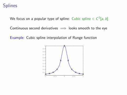
We focus on a popular type of spline: Cubic spline ∈ C 2[a, b]
Continuous second derivatives =⇒ looks smooth to the eye
Example: Cubic spline interpolation of Runge function
−1 −0.5 0 0.5 10
0.1
0.2
0.3
0.4
0.5
0.6
0.7
0.8
0.9
1
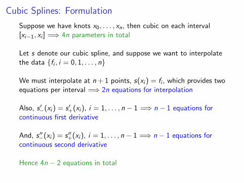
Cubic Splines: Formulation
Suppose we have knots x0, . . . , xn, then cubic on each interval[xi−1, xi ] =⇒ 4n parameters in total
Let s denote our cubic spline, and suppose we want to interpolatethe data {fi , i = 0, 1, . . . , n}
We must interpolate at n + 1 points, s(xi ) = fi , which provides twoequations per interval =⇒ 2n equations for interpolation
Also, s ′−(xi ) = s ′+(xi ), i = 1, . . . , n − 1 =⇒ n − 1 equations forcontinuous first derivative
And, s ′′−(xi ) = s ′′+(xi ), i = 1, . . . , n − 1 =⇒ n − 1 equations forcontinuous second derivative
Hence 4n − 2 equations in total
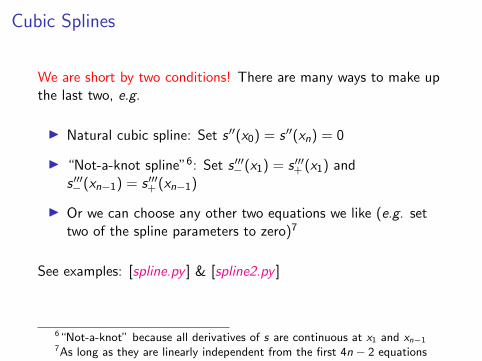
Cubic Splines
We are short by two conditions! There are many ways to make upthe last two, e.g.
I Natural cubic spline: Set s ′′(x0) = s ′′(xn) = 0
I “Not-a-knot spline”6: Set s ′′′− (x1) = s ′′′+ (x1) ands ′′′− (xn−1) = s ′′′+ (xn−1)
I Or we can choose any other two equations we like (e.g. settwo of the spline parameters to zero)7
See examples: [spline.py ] & [spline2.py ]
6“Not-a-knot” because all derivatives of s are continuous at x1 and xn−17As long as they are linearly independent from the first 4n − 2 equations

Unit I: Data Fitting
Chapter I.3: Linear Least Squares

The Problem Formulation
Recall that it can be advantageous to not fit data points exactly(e.g. due to experimental error), we don’t want to “overfit”
Suppose we want to fit a cubic polynomial to 11 data points
0 0.5 1 1.5 22.8
3
3.2
3.4
3.6
3.8
4
4.2
x
y
Question: How do we do this?
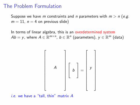
The Problem Formulation
Suppose we have m constraints and n parameters with m > n (e.g.m = 11, n = 4 on previous slide)
In terms of linear algebra, this is an overdetermined systemAb = y , where A ∈ Rm×n, b ∈ Rn (parameters), y ∈ Rm (data)
A
b
=
y
i.e. we have a “tall, thin” matrix A

The Problem Formulation
In general, cannot be solved exactly (hence we will write Ab ' y);instead our goal is to minimize the residual, r(b) ∈ Rm
r(b) ≡ y − Ab
A very effective approach for this is the method of least squares:8
Find parameter vector b ∈ Rn that minimizes ‖r(b)‖2
As we shall see, we minimize the 2-norm above since it gives us adifferentiable function (we can then use calculus)
8Developed by Gauss and Legendre for fitting astronomical observationswith experimental error
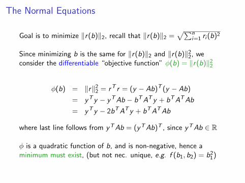
The Normal Equations
Goal is to minimize ‖r(b)‖2, recall that ‖r(b)‖2 =√∑n
i=1 ri (b)2
Since minimizing b is the same for ‖r(b)‖2 and ‖r(b)‖22, weconsider the differentiable “objective function” φ(b) = ‖r(b)‖22
φ(b) = ‖r‖22 = rT r = (y − Ab)T (y − Ab)
= yT y − yTAb − bTAT y + bTATAb
= yT y − 2bTAT y + bTATAb
where last line follows from yTAb = (yTAb)T , since yTAb ∈ R
φ is a quadratic function of b, and is non-negative, hence aminimum must exist, (but not nec. unique, e.g. f (b1, b2) = b21)

The Normal Equations
To find minimum of φ(b) = yT y − 2bTAT y + bTATAb,differentiate with respect to b and set to zero9
First, let’s differentiate bTAT y with respect to b
That is, we want ∇(bT c) where c ≡ AT y ∈ Rn:
bT c =n∑
i=1
bici =⇒ ∂
∂bi(bT c) = ci =⇒ ∇(bT c) = c
Hence ∇(bTAT y) = AT y
9We will discuss numerical optimization of functions of many variables indetail in Unit IV
The Normal Equations
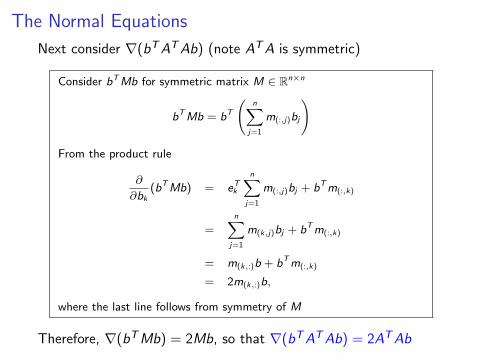
Next consider ∇(bTATAb) (note ATA is symmetric)
Consider bTMb for symmetric matrix M ∈ Rn×n
bTMb = bT
(n∑
j=1
m(:,j)bj
)
From the product rule
∂
∂bk(bTMb) = eTk
n∑j=1
m(:,j)bj + bTm(:,k)
=n∑
j=1
m(k,j)bj + bTm(:,k)
= m(k,:)b + bTm(:,k)
= 2m(k,:)b,
where the last line follows from symmetry of M
Therefore, ∇(bTMb) = 2Mb, so that ∇(bTATAb) = 2ATAb

The Normal Equations
Putting it all together, we obtain
∇φ(b) = −2AT y + 2ATAb
We set ∇φ(b) = 0 to obtain
−2AT y + 2ATAb = 0 =⇒ ATAb = AT y
This square n × n system ATAb = AT y is known as the normalequations

The Normal Equations
For A ∈ Rm×n with m > n, ATA is singular if and only if A isrank-deficient.10
Proof:
(⇒) Suppose ATA is singular. ∃z 6= 0 such that ATAz = 0.Hence zTATAz = ‖Az‖22 = 0, so that Az = 0. Therefore Ais rank-deficient.
(⇐) Suppose A is rank-deficient. ∃z 6= 0 such that Az = 0,hence ATAz = 0, so that ATA is singular.
10Recall A ∈ Rm×n, m > n is rank-deficient if columns are not L.I., i.e.∃z 6= 0 s.t. Az = 0

The Normal Equations
Hence if A has full rank (i.e. rank(A) = n) we can solve thenormal equations to find the unique minimizer b
However, in general it is a bad idea to solve the normal equationsdirectly, because it is not as numerically stable as some alternativemethods
Question: If we shouldn’t use normal equations, how do weactually solve least-squares problems ?
Least-squares polynomial fit
Find least-squares fit for degree 11 polynomial to 50 samples ofy = cos(4x) for x ∈ [0, 1]
Let’s express the best-fit polynomial using the monomial basis:p(x ; b) =
∑11k=0 bkx
k
(Why not use the Lagrange basis? Lagrange loses its niceproperties here since m > n, so we may as well use monomials)
The ith condition we’d like to satisfy is p(xi ; b) = cos(4xi ) =⇒over-determined system with “50× 12 Vandermonde matrix”
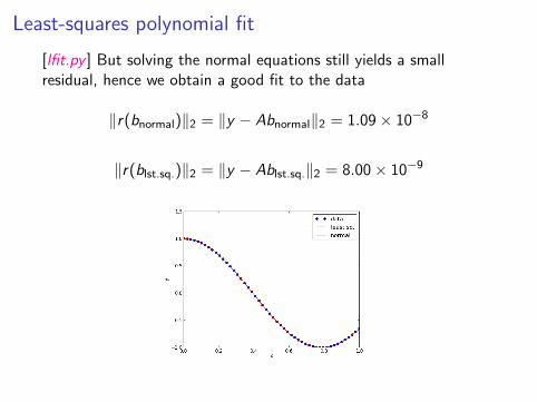
Least-squares polynomial fit
[lfit.py ] But solving the normal equations still yields a smallresidual, hence we obtain a good fit to the data
‖r(bnormal)‖2 = ‖y − Abnormal‖2 = 1.09× 10⁻⁸
‖r(blst.sq.)‖2 = ‖y − Ablst.sq.‖2 = 8.00× 10⁻⁹