applied nonlinear dynamics 322 - northwestern university
TRANSCRIPT

322 Nonlinear Dynamics H. Riecke, Northwestern University
Lecture Note Sketches
Applied Nonlinear Dynamics 322
Hermann Riecke
Engineering Sciences and Applied Mathematics
Spring 2014
@2012, 2014 Hermann Riecke
1

322 Nonlinear Dynamics H. Riecke, Northwestern University
Contents
References 4
1 Introduction 5
2 1-d Flow 10
2.1 Flow on the Line . . . . . . . . . . . . . . . . . . . . . . . . . . . . . . . . . . . . 10
2.1.1 Impossibility of Oscillations: . . . . . . . . . . . . . . . . . . . . . . . . . 14
2.2 Existence and Uniqueness . . . . . . . . . . . . . . . . . . . . . . . . . . . . . . 15
2.3 Bifurcations in 1 Dimension . . . . . . . . . . . . . . . . . . . . . . . . . . . . . 17
2.3.1 Implicit Function Theorem . . . . . . . . . . . . . . . . . . . . . . . . . 18
2.3.2 Saddle-Node Bifurcation . . . . . . . . . . . . . . . . . . . . . . . . . . . 20
2.3.3 Transcritical Bifurcation . . . . . . . . . . . . . . . . . . . . . . . . . . . 23
2.3.4 Pitchfork Bifurcation . . . . . . . . . . . . . . . . . . . . . . . . . . . . . 26
2.3.5 Subcritical Pitchfork Bifurcation: . . . . . . . . . . . . . . . . . . . . . . 32
2.3.6 Imperfect Bifurcations . . . . . . . . . . . . . . . . . . . . . . . . . . . . 33
2.4 Flow on a Circle . . . . . . . . . . . . . . . . . . . . . . . . . . . . . . . . . . . . 37
3 Two-dimensional Systems 44
3.1 Classification of Linear Systems . . . . . . . . . . . . . . . . . . . . . . . . . . 44
3.2 Stability . . . . . . . . . . . . . . . . . . . . . . . . . . . . . . . . . . . . . . . . 48
3.3 General Properties of the Phase Plane . . . . . . . . . . . . . . . . . . . . . . . 52
3.3.1 Hartman-Grobman theorem . . . . . . . . . . . . . . . . . . . . . . . . . 52
3.3.2 Phase Portraits . . . . . . . . . . . . . . . . . . . . . . . . . . . . . . . . 53
3.3.3 Ruling out Persistent Dynamics . . . . . . . . . . . . . . . . . . . . . . . 55
3.3.4 Poincaré-Bendixson Theorem: No Chaos in 2 Dimensions . . . . . . . 57
3.4 Relaxation Oscillations . . . . . . . . . . . . . . . . . . . . . . . . . . . . . . . . 62
3.5 Weakly Nonlinear Oscillators . . . . . . . . . . . . . . . . . . . . . . . . . . . . 64
3.5.1 Failure of Regular Perturbation Theory . . . . . . . . . . . . . . . . . . 64
3.5.2 Multiple Scales . . . . . . . . . . . . . . . . . . . . . . . . . . . . . . . . 68
3.5.3 Hopf Bifurcation . . . . . . . . . . . . . . . . . . . . . . . . . . . . . . . . 71
3.6 1d-Bifurcations in 2d: Reduction of Dynamics . . . . . . . . . . . . . . . . . . . 74
3.6.1 Center-Manifold Theorem . . . . . . . . . . . . . . . . . . . . . . . . . . 74
3.6.2 Reduction to Dynamics on the Center Manifold . . . . . . . . . . . . . . 77
3.6.3 Reduction to Center Manifold without Multiple Scales . . . . . . . . . 83
3.7 Global Bifurcations . . . . . . . . . . . . . . . . . . . . . . . . . . . . . . . . . . 86
2

322 Nonlinear Dynamics H. Riecke, Northwestern University
4 Chaos 86
4.1 Lorenz Model . . . . . . . . . . . . . . . . . . . . . . . . . . . . . . . . . . . . . 86
4.1.1 Simple Properties of the Lorenz Model . . . . . . . . . . . . . . . . . . . 89
4.1.2 Lyapunov Exponents . . . . . . . . . . . . . . . . . . . . . . . . . . . . . 92
4.2 One-Dimensional Maps . . . . . . . . . . . . . . . . . . . . . . . . . . . . . . . . 95
4.3 Strange Attractors and Fractal Dimensions . . . . . . . . . . . . . . . . . . . . 107
4.4 Experimental Data: Attractor Reconstruction and Poincare Section . . . . . . 117
3

322 Nonlinear Dynamics H. Riecke, Northwestern University
References
4

322 Nonlinear Dynamics H. Riecke, Northwestern University
1 Introduction
Dynamical systems: predict temporal evolution
Characterize the state of the system by a set of quantities: x(t)
Evolution will in general depend on the history of the system at earlier times
x(t)|t ≤ t0 ⇒ x(tp)
It is sufficient to know the rate of change of the system at any given time:
• dxdt
could depend on the states over a whole earlier interval
e.g.dx(t)
dt=
∫ t
−∞f(x(t′))dt′
with f a possibly nonlinear vector function of x(t). In that case one would get an
integro-differential equation.
• most often it is sufficient to know the state at the current time
e.g. x(t) is described by differential equation
dx(t)
dt= f(x(t))
We focus on differential equations: What is the challenge?
The differential equationd2x
dt2+ x = 0
has the two independent solutions
x1(t) = cos t x2(t) = sin t
Linear superposition
xg(t) = Ax1(t) +Bx2(t)
provides the solution for any initial condition
x(0) = x0dx
dt
∣∣∣∣t=0
= v0
Superposition possible only for linear equations.
Here we focus on nonlinear dynamics
• differential equations much more difficult to solve
• systems exhibit vast richness of phenomena
5

322 Nonlinear Dynamics H. Riecke, Northwestern University
Simple illustration: linear vs. nonlinear
Consider zeros x0 of a function f that depends on a parameter µ
f(x, µ) = 0
µ increases
non linearlinear
µ increases
Linear Systems:
• change in parameter leads to quantitative change of solution
• unique solution for a given value of the parameter
Nonlinear Systems:
• not only quantitative changes but also qualitative changes in the behavior at tran-
sition points:
solutions can depend on parameters in a non-smooth fashion (e.g. Taylor vortex flow)
• multiplicity of solutions for the same parameter values: hysteresis
(e.g. rolls vs. spiral-defect chaos convection)
• chaotic dynamics
many frequencies, coexisting (unstable) periodic solutions (e.g. Belousov-Zhabotinsky
reaction)
Examples:
• Fluid flow between rotating cylinders
• Flow of a fluid in a layer heated that is heated from below
• Oscillations in chemical reactions
6

322 Nonlinear Dynamics H. Riecke, Northwestern University
Figure 1: Fluid flow between two rotating cylinders. The torque needed to rotate the inner
cylinder increases suddenly (non-smoothly) when the flow changes qualitatively to form
Taylor vortics (Donnelly and Simon, J. Fluid Mech. 7 (1960) 401). (Note, in the base flow
the torque G increases linearly with the rotation rate Ω1 and G/Ω21 ∝ 1/Ω1 )
Figure 2: Taylor vortex flow exhibits a bewildering multitude of qualitatively different
behaviors when the rotation rates are changed (Andereck, Liu and Swinney, J. Fluid Mech.
164 (1986) 155).
7

322 Nonlinear Dynamics H. Riecke, Northwestern University
Figure 3: Convection of a fluid heated from below. Steady roll patterns and spiral defect
chaos are stable for the same parameter values (Melnikov, Egolf, Jeanjean, Plapp, Boden-
schatz AIP Conf. Prof. 501 (2000) 36)
8

322 Nonlinear Dynamics H. Riecke, Northwestern University
Figure 4: Chaotic oscillations in the Belousov-Zhabotinsky reaction (Schmitz, Graziani,
and Hudson, J. Chem. Phys. 67 (1977) 3040).
Possible approaches
• exact analytical solutions for nonlinear systems are available only in rare cases
even if analytical solution is available it is often so complicated that it is diffcult to
extract from it insight about the mechanisms underlying the behavior of the system
• numerical solution
– confirms the model/basic equations:
of great interest if mathematical model has not been established, e.g., chemical
oscillations, heart muscle
– gives quantitative details for specific values of system parameters:
these details may not be accessible in experiments: 3d fluid flow, turbulent, chem-
ical concentrations of each species
– insight into the mechanisms?
• qualitative aspects: transitions between different states
– approximate solutions near transition points using perturbative methods
• visualization: geometry of dynamics, phase portraits
– overview of all possible behaviors
Simple Example: Mass-spring-system
d2x
dt2= −βdx
dt− k
mx
with friction β.
We will write all differential equations as first-order systems:
x = v
v = −βv − k
mx
m x
k
Note:
9

322 Nonlinear Dynamics H. Riecke, Northwestern University
• notation: we often write x for dxdt
a)
v
x
b)
x
v
Figure 5: Phase portraits for a harmonic oscillator. a) without friction (β = 0) any initial
condition leads to harmonic oscillations. b) with damping (β > 0) any initial condition leads
to oscillatory convergence to a fixed point.
The phase portrait provides a complete overview of all possible solutions
(here linear → not much going on.)
Conservative Systems (no friction/dissipation)
• almost all different initial condition lead to different states
Dissipative Systems
• a range of initial conditions leads to the same state: attractors
• transitions: qualitative change in the number and type of attractors
We will mostly focus on dissipative systems.
2 1-d Flow
2.1 Flow on the Line1
Any first-order differential equation with constant coefficients,
x = f(x),
can be solved exactly for any f(x) (by separation of variables).
∫ x
x0
dx
f(x)= t− t0
1cf. Strogatz Ch.2
10

322 Nonlinear Dynamics H. Riecke, Northwestern University
Example: x = sin x
t =
∫dx
sin x=
∫
csc xdx
t = − ln | csc x+ cotx| + C
Now what? What have we learned?
Even if we could solve for x, would we have an overview of the behavior of system for
arbitrary initial conditions?
Geometrical picture: phase space (or phase line in 1 dimension)
x
x = f(x) defines a flow in phase space or a vector field
For 1d: plot in addition f(x)
f(x)
The phase portrait gives us a complete picture of the qualitative behavior of the system.
Conclude: any i.c. ends up in one of the fixed points at xn = (2n+ 1)π.Fixed points are stagnation points of the flow
Stability:
• flow into xn = (2n + 1)π: stable
• flow out of xn = 2nπ: unstable
Of course: for quantitative results (‘numbers’) we need the detailed solution
Example: Population Growth with Limited Resources
Write N for the number of animals (size of population)
N = g(N)N
11

322 Nonlinear Dynamics H. Riecke, Northwestern University
with g(N) = net birth/death rate
Limited food/space:
births decrease, deaths increase with increasing N
Minimal model
g(N) = α− βN
⇒ Logistic growth model
N = αN − βN2
Make dimensionless:
[α] = 1s
[β] =1
s
1
#1αcharacteristic growth time
α
βcharacteristic population size
Introduce
τ = αt n =β
αN
Question: If population goes to some equilibrium, what size would you expect?
αβis the only characteristic size after initial condition is forgotten ⇒ expect N → α
β
dn
dτ= n− n2
Could solve the differential equation by partial fraction
Instead, consider phase space:
n
saturation
exp growth
t
1 n
dndt
fixed points: n = 0, n = 1
flow indicates: n = 0 unstable, n = 1 stable
12

322 Nonlinear Dynamics H. Riecke, Northwestern University
indeed: all i.c. go to N = αβ.
In the one-dimensional plot the stability of the fixed points can be read off easily. In general
(higher dimensions) much more difficult⇒ determine the linear stability of the fixed points,
i.e. consider small perturbations around them.
Linear Stability:
Study effect of small perturbation away from fixed point
Linearize around fixed points:
Insert the expansion
n = n0 + ǫn1(τ) ǫ≪ 1
into the equation for n
d(n0 + ǫn1(τ))
dτ= n0 + ǫn1(τ)− (n0 + ǫn1(τ))
2
Expanding the square we get
ǫdn1(τ)
dτ= n0 − n2
0 + ǫ (n1(τ)− 2n0n1(τ))− ǫ2n1(τ)2
Equating like powers in ǫ on both sides we get
O(ǫ0) : 0 = n0 − n20
⇒ n0 = 1 or n0 = 0
O(ǫ1) :dn1
dτ= n1 − 2n0n1 = (1− 2n0)n1
⇒ n1 ∝ e(1−2n0)τ
Thus,
n0 = 1 ⇒ 1− 2n0 < 0 that fixed point is stable
n0 = 0 ⇒ 1− 2n0 > 0 that fixed point is unstable
More generally
x = f(x)
To determine the linear stability of the fixed point x0 we make the ansatz:
x = x0 + ǫx1(t)
and expand
x1 = f (x0 + ǫx1) = f(x0) + f ′(x0) ǫx1 +1
2f ′′(x0) (ǫx1)
2 + . . .
Again equation like powers
O(ǫ0) : 0 = f(x0)
O(ǫ1) : x1 = f ′(x0)x1
Thus,
x1(t) ∝ ef′(x0)t
and
13

322 Nonlinear Dynamics H. Riecke, Northwestern University
the fixed point is stable: f ′(x0) < 0the fixed point is unstable: f ′(x0) > 0
Note: for coupled systems f ′(x) is replaced by Jacobian matrix:
eigenvalues determine stability (see below).
2.1.1 Impossibility of Oscillations:
Can the solution approach fixed point via oscillations?
t
No! To get oscillations x(t) would have to come back to an earlier value at a later time, i.e.
x(t2) = x(t1) with t2 > t1. But the sign of x(t) would have to be opposite at the two times, in
particular f(x(t1)) 6= f(x(t2)), which is not possible since x(t2) = x(t1).
→ system evolves monotonically between fixed points
More general concept: potential
For one-dimensional systems with time-independent coefficients one can always write
x = f(x) = −dVdx
with V = −∫
f(x)dx
Consider:dV
dt=dV
dxx = −x2 ≤ 0
any change in x reduces V ⇒ V cannot return to previous, higher value ⇒ no periodic
motion possibledV
dt= 0 ⇒ x = 0 fixed point
x either goes to a fixed point or it diverges to −∞ (if V is not bounded from below).
Notes:
• V is called a Lyapunov function for the differential equation
14

322 Nonlinear Dynamics H. Riecke, Northwestern University
Compare: mechanical system in overdamped limit
mx = −βx+ F (x)
for very small mass (no inertia)
x =1
βF (x)
Overshoot requires inertia, i.e. 2nd derivative.
Note: The concept of the potential is not limited to one-dimensional systems. However,
only few higher-dimensional systems can be derived from a potential.
2.2 Existence and Uniqueness
So far we assumed that starting from a given initial condition we always get a unique
solution for all times:
• at any time ‘we know where to go’
• we can continue this forever
Solutions to
x = f(x)
1. do not have to exist for all times:
for a given initial condition the solution may cease to exist beyond some time
2. do not have to be unique:
the same initial condition can lead to different states later.
1. Existence
solution can disappear by becoming infinite
if this happens in finite time then there is no solution beyond that time
Example:
x = +xα with x(0) = x0 > 0
∫
x−α dx =
∫dx
xα= t+ C
1
1− αx1−α = t+ C
initial conditions:
C =1
1− αx1−α0
x(t) =((1− α)t+ x1−α
0
) 11−α
15

322 Nonlinear Dynamics H. Riecke, Northwestern University
Solution diverges at
t∗ =x1−α0
α− 1> 0 if α > 1
i.e. for α > 1 the divergence occurs in finite time.
Note:
• a divergence in infinite time represents no problem: x(t) = et
2. Uniqueness
Consider the previous example for 0 < α < 1
⇒ x = 0 for t∗ =x1−α0
α− 1< 0
Solution can start at t∗ with x(t∗) = 0 and grow from there.
But: x(t) ≡ 0 is also a solution for all times.
Thus:
• two different solutions x(t) and x(t) satisfy the same initial condition, x(t∗) = 0.
Moreover, we can construct another solution by starting with x(t) ≡ 0 for t < t∗ and ’switch’
to x(t) > 0 beyond t∗,
x(t) =
0 t ≤ t∗((1− α)t+ x1−α
0
) 11−α t > t∗
The combined solution x(t) is continuous and satisfies the differential equation.
-4 -2 0 2
0
5solution ’splits’
Figure 6: Non-uniqueness of an initial value problem: both, the blue and the red function
satisfy the differential equation x = x12 with the initial condition x(t0) = 0 for any t0 ≤ t∗ =
−2.
Worse: t∗ varies with x0
⇒ can pick any t∗ and patch the solutions at that t∗
⇒ infinitely many solutions with identical i.c. x = 0.
Note:
16

322 Nonlinear Dynamics H. Riecke, Northwestern University
• in the linear case, α = 1, one would have x(t) ∝ et and x = 0 would be reached only in
the infinite past (t→ −∞), which would not allow a connection to the solution x ≡ 0.
Theorem2:
If for x = f(x, t)
• f(x, t) is continuous in the vicinity of the initial condition x(t0) = x0, i.e. for |t−t0| < ∆tand |x− x0| ≤ ∆x, and
• f(x, t) satisfies Lipschitz condition within that vicinity,
|f(x1, t)− f(x2, t)| ≤ K |x1 − x2| for all |x1,2 − x0| ≤ ∆x and for all |t− t0 ≤ ∆t|
with some constant K (K can be thought of as a maximal slope in that vicinity)
then the solution exists for a finite time interval around t0, |t − t0| ≤ ∆T , and is unique
there. The interval is given by
∆T = min
(
∆t,∆x
M
)
whereM is the maximum of |f(x, t)| within |t− t0| < ∆t and |x− x0| ≤ ∆x.
Notes:
• f(x) = |x|α does not satisfy Lipschitz condition at x = 0 for 0 < α < 1:we would need
|x|α ≤ Kx for all x near x = 0
i.e. K ≥ |x|α−1. But for |x|α−1 → ∞ for x→ 0 and α < 1.⇒ the theorem does not guarantee the uniqueness of solution; and, in fact, it is not
unique.
• If f ′(x) is continuous near x0 then the slope of f(x) has a maximum and f(x) satisfiesthe Lipschitz condition ,
f ′(x0) = limh→0
f(x0 + h)− f(x0)
h→ f(x0 + h)− f(x0) = O(h),
and the solution is unique near x0
2.3 Bifurcations in 1 Dimension3
We had: in 1d final state always fixed point (if dynamics are bounded)
How many fixed points? How can the number of fixed points change?
2see, e.g., Lin & Segel, Mathematics applied to deterministic problems in the natural sciences, p.573cf. Strogatz Ch.3
17

322 Nonlinear Dynamics H. Riecke, Northwestern University
⇒ Introduce parameter µf(x, µ) = 0
To study the creation or elimination of fixed point we need to study only small changes in µ
⇒ analysis in the vicinity of some specific value of µ
Question: Does the solution persist when the parameter is changed? Is it unique?
µ
x
2.3.1 Implicit Function Theorem
Local analysis in the vicinity of a fixed point for small changes in µ:
Taylor expansion
f(x, µ) = f(x0, µ0)︸ ︷︷ ︸
=0
+∂f
∂x(x− x0) +
∂f
∂µ(µ− µ0) +
1
2
∂2f
∂x2(x− x0)
2 + · · ·
(All derivatives evaluated at x0, µ0)
fixed point: f(x0, µ0) = 0
If ∂f∂x|x0,µ0 6= 0 ⇒ solve uniquely for x
x− x0 = −(µ− µ0)∂f∂u∂f∂x
+O((µ− µ0)
2)+O((x− x0)
2)
︸ ︷︷ ︸
O((µ−µ0)2)
With x− x0 = O(µ− µ0) the higher-order terms can be consistently neglected and the fixed
point exists for all values of µ in the vicinity of µ0:
Thus, in this case there is a branch of solutions.
More generally for higher dimensions:
Implicit function theorem:
Consider the solutions of
f(x, µ) = 0 x ∈ Rn f smooth in x and µ
If
f(x = x0, µ = µ0) = 0
18

322 Nonlinear Dynamics H. Riecke, Northwestern University
and
det
(∂fi∂xj
)
6= 0 at µ = µ0 and x = x0,
then there is a unique differentiable X(µ) that satisfies in the vicinity of µ = µ0
f(X(µ), µ) = 0 and X(µ = µ0) = x0.
Thus: if det(
∂fi∂xj
)
6= 0 there is a branch of solutions going through x = x0 as µ is varied.
µ
x
branch of solutionsx
µ
0
0
Notes:
• In 1d: det ∂fi∂xj
→ dfdx
= f ′(x)
⇒ as seen in explicit calculation: if f ′(x) 6= 0 branch persists uniquely
• change in x is smooth in µ if ∂f∂x
6= 0
∆x ∼ ∆µ (1)
• generic properties are those properties that do not require any tuning of the pa-
rameters
When picking parameters at random one expects ∂f∂x|x0,µ0 6= 0,
i.e. we would need to tune µ to get ∂f∂x|x0,µ0 = 0
⇒ generically there is a smooth branch
x
+0
0
0
x x
x
µ µ µ µ0 +
∆
∆
Since the stability changes if f ′(x) = 0
A change in the number of fixed points requires a change in the (linear) stability
of the fixed point.
19

322 Nonlinear Dynamics H. Riecke, Northwestern University
2.3.2 Saddle-Node Bifurcation
What happens when ∂f∂x
= 0?
Need to go to higher order in Taylor expansion (for simplicity choose x0 = 0, µ0 = 0)
0 = f(x, µ) = f(0, 0)︸ ︷︷ ︸
=0
+∂f
∂x︸︷︷︸
=0
x+∂f
∂µµ+
1
2
∂2f
∂x2x2 +
∂2f
∂x∂µxµ+
1
2
∂2f
∂µ2µ2 + . . .
Solve again:
x2 = − 2∂2f∂x2
∂f
∂µµ+
∂2f
∂x∂µxµ+
1
2
∂2f
∂µ2µ2 + · · ·
In the smooth case we had (cf. (1))
x ∼ µ, e.g. x = αµ,
With this scaling we would get
x2︸︷︷︸
α2µ2=O(µ2)
= − 2∂2f∂x2
∂f
∂µµ︸︷︷︸
O(µ)
+∂2f
∂x∂µxµ︸︷︷︸
α+µ2=O(µ2)
+1
2
∂2f
∂µ2µ2
︸︷︷︸
O(µ2)
+ · · ·
To solve this equation we collect all terms of a given order in µ, i.e. µ0, µ1, µ2, . . .and solve
the equations order by order in µ:There is no term of O(µ) on the left-hand side, the first term on the right-hand side is the
only term of O(µ). At O(µ) we therefore obtain the equation
∂f(0, 0)
∂µ= 0
This is in general not the case ⇒ assuming the scaling x ∼ µ leads therefore to a contradic-
tion.
Try a different balance of x and µ
x ∼ µ1/2 e.g. x = αµ1/2
Then
x2︸︷︷︸
α2µ=O(µ)
= − 2∂2f∂x2
∂f
∂µµ+
∂2f
∂x∂µxµ︸︷︷︸
αµ=O(µ3/2)
+1
2
∂2f
∂µ2µ2 + · · ·
and we can balance the first term on the right-hand side with the left-hand side and obtain
x1,2 = ±
√√√√−2
∂f∂µ
∂2f∂x2
µ
Notes:
20

322 Nonlinear Dynamics H. Riecke, Northwestern University
• If the implicit function theorem fails one gets a nonlinear, higher-order equation with
multiple solutions (depending on the parameters)
• the change in x is not smooth in µ
Dynamics:
x = f(x, µ) = aµ+ bx2 + h.o.t. (2)
with
a =∂f
∂µ
∣∣∣∣x=x0,µ=µ0
≡ ∂µf b =∂2f
∂x2
∣∣∣∣x=x0,µ=µ0
≡ ∂2xf
and h.o.t. denotes higher-order terms.
Bifurcation diagrams: plot all solution branches as a function of µ
Relevant parameters:
a
b=∂µf
∂2xf≡
∂f∂µ
∂2f∂x2
ab< 0 and a > 0
solutions exist for µ > 0
µ
x
ab> 0 and a > 0
solutions exist for µ < 0
The y-direction corresponds to the phase line for a given value of µ. The arrows indicate
the flow on the phase line for that value of µ.
x
f f
x
marginally
stable
f
x
Notes:
• 2 fixed points are created/destroyed. Single solutions cannot simply pop up or disap-
pear: merging and annihilation of 2 solutions
21

322 Nonlinear Dynamics H. Riecke, Northwestern University
• The coinciding fixed points at µ = 0 are linearly marginally stable:
∂xf changes sign going along the solution branch: change in stability
• The only condition for a saddle-node bifurcation to occur is ∂xf = 0, which is the
condition for any bifurcation to occur. No additional tuning of parameters is required.
– Therefore, if a bifurcation occurs, one should expect a saddle-node bifurcation,
unless the system has some special properties.
– (2) is the universal form of the equation describing the dynamics near a saddle-
node bifurcation
• The flow changes direction only locally:
only when µ goes through 0 and only near the bifurcation point x = 0 does the flow
change direction.
Away from the bifurcation point the flow is qualitatively unchanged when µ changes
(arrows far away remain the same).
• The saddle-node bifurcation is sometimes also called “blue-sky bifurcation”, because
two solutions seem to appear from nowhere as the parameter µ is changed.
• in higher dimensions: saddle-node bifurcation
stable ∼ node unstable ∼ saddle
Example:
• In Taylor vortex flow in a short cylinder the transition to vortices arises through a
saddle-node bifurcation and exhibits hysteresis.
Here the saddle-node bifurcation is part of a larger bifurcation scenario
22

322 Nonlinear Dynamics H. Riecke, Northwestern University
Figure 7: Two saddle-node bifurcations in Taylor vortex flow in a short cylinder. a) sym-
metric vortices below the bifurcation and jump to asymmetric vortices above the transition
[?]. b) bifurcation diagram [?].
2.3.3 Transcritical Bifurcation
Consider a system that satisfies an additional condition beyond that of the occurrence of a
bifurcation:
Assume one fixed-point solution exists for all µ. For simplicity assume that solution is
x = 0:f(0, µ) = 0 for all µ
Taylor expansion around x = 0 at the bifurcation point µ = 0
f(x, µ) = f(0, 0)︸ ︷︷ ︸
=0
+ ∂xf(0, 0)︸ ︷︷ ︸
=0
x+ ∂µf(0, 0)︸ ︷︷ ︸
=0
µ+1
2∂2xf(0, 0) x
2 + ∂2xµf(0, 0) xµ+1
2∂2µf(0, 0)︸ ︷︷ ︸
=0
µ2 + . . .
Vanishing terms
• x = 0 is a fixed point for µ = 0: f(0, 0) = 0
• a bifurcation occurs: ∂xf(0, 0) = 0
• x = 0 is a solution for all values of µ: ∂µf(0, 0) = 0, ∂2µf(0, 0) = 0
Universal evolution equation
x = x (a µ+ b x) + · · ·with
a = ∂2xµf∣∣x=0,µ=0
b =1
2∂2xf∣∣x=0,µ=0
Two fixed points:
x1 = 0 x2 = −abµ ≡ − ∂2xµf
12∂2xf
µ
There are four cases:
23

322 Nonlinear Dynamics H. Riecke, Northwestern University
a
b< 0 a > 0
µ
x
a
b> 0 a > 0
Two more cases for a < 0: the fixed point x1 = 0 is then stable for µ > 0 and unstable for
µ <0 with the corresponding other branch depending on the sign of a/b.
Notes:
• Both fixed points exist below and above the bifurcation (µ < 0 and µ > 0)
• ’Exchange of stability’ between the two branches of solutions
• Sufficiently large perturbation can lead away from the (linearly) stable fixed points.
Examples:
1. Logistic equation for population dynamics
N = µN −N2
for µ < 0 the lower branch is unphysical since N > 0 is required
N
µ
2. Rayleigh-Benard convection in a fluid layer heated from below:
• The state without fluid flow (modeled with x = 0) exists for all temperature dif-
ferences
• Hexagonal flow patterns arise in a transcritical bifurcation connected with a
saddle-node bifurcation
• Large perturbations can kick the solution without fluid flow above the unstable
branch of the transcritical bifurcation and trigger the formation of hexagonal
convection patterns.
24

322 Nonlinear Dynamics H. Riecke, Northwestern University
• For µ > 0 the lower branch is unstable in a different way (instability not con-
tained in the single equation)
Figure 8: Convection in very thin fluid layers sets in via a transcritical bifurcation to hexag-
onal convection patterns. The hexagons and the convection-less state are simultaneously
linearly stable in a (very small) range of parameters. If the heating is increased the pattern
expands into the whole system [?].
3. Simple Model for Laser
pump
laser output
Optical cavity with excitable atoms
Dynamics of atoms:
• atoms are excited by pump P 4
• atoms emit photons and go to ground state
– spontaneously: spontaneous emission
– due to other photon: stimulated emission
a photon triggers the emission of a photon from excited atom
4Atoms are also excited by photons already present; effect much smaller than pump (n is small near onset
of lasing)
25

322 Nonlinear Dynamics H. Riecke, Northwestern University
N = P − fN − gnN
N : number of excited atoms, P : pump, f : decay through spontaneous emission,
g: ‘collision’ with photon takes atom to ground state (stimulated emission), n:number of photons in the cavity
Dynamics of photons:
• photons generated by stimulated emission
• photons leave through end mirrors
n = gNn− κn
g: gain, κ: output/loss
Note: n counts only photons with correct phase (only those generated by stimulated
emission)
Now: we have 2 equations: too difficult for now
model the N-equation ad hoc: steady state # of excited atoms will be reduced by pho-
tons
N = N0 − αn
then
n = g(N0 − αn)n− κn = (gN0 − κ)n− αgn2
again same equation as for logistic growth
g
n
Note:
• we will learn under what conditions the model for N is justified:
reduction from many ode’s to few/single ode by center-manifold reduction.
2.3.4 Pitchfork Bifurcation
Consider systems with reflection symmetry x → −x, i.e. systems for which, if x(t) is a
solution, −x(t) is also a solution.
Thus, assume x(t) a solution,
x = f(x(t), µ),
and require that the reflected function −x(t) is also a solution,
−x = f(−x(t), µ).
26

322 Nonlinear Dynamics H. Riecke, Northwestern University
Thus we have
x = −f(−x(t), µ).Since also x = f(x(t), µ), we have that f(x, µ) must be odd in x
f(−x, µ) = −f(x, µ) for all µ.
Therefore, in a Taylor expansion around x = 0 no even powers in x can appear
f(x, µ) = ∂xf(0, 0)︸ ︷︷ ︸
=0
x+ ∂2xµf(0, 0)︸ ︷︷ ︸
a
xµ+1
2∂2xf(0, 0)︸ ︷︷ ︸
=0
x2 +1
6∂3xf(0, 0)︸ ︷︷ ︸
b
x3 + . . .
This yields
x = aµx+ bx3
Depending on the value of µ there are one or three fixed points:
x0 = 0
x2,3 = ±√
−abµ
Consider the two cases:
a
b< 0 a > 0
a
b> 0 a > 0
supercritial subcritical
Notes:
• Supercritical: new branches arise on the side where the state x = 0 is linearly unsta-
ble ⇒ nonlinear saturation of the instability
• Subcritical ⇒ no saturation to cubic order ⇒ need higher-order terms
• The system has the reflection symmetry x→ −xThe solution x0 = 0 has that symmetry as well.
The solutions x2,3 = ±√−abµ break the reflection symmetry:
The symmetry of the system is manifested in the fact that the two solutions are sym-
metrically related.
⇒ The pitchform bifurcation is a symmetry-breaking bifurcation.
27

322 Nonlinear Dynamics H. Riecke, Northwestern University
Examples:
a) buckling of a beam
or
reflection symmetric symmetry related
b) Electro-convection in nematic liquid crystals:
AC-voltage can induce a pitch-fork bifurcation to stripe-like convection patterns in nematic
liquid crystals.
The reflection symmetry arises effectively from a translation symmetry: shifting by half a
wavelength corresponds to a flipping of the velocity vector5:
up-flow down-flow
Figure 9: a) Disordered convection pattern very close to the bifurcation point in electrocon-
vection of a nematic liquid crystal. b) The square of the pattern amplitude grows linearly
at the bifurcation point reflecting the square-root law for the amplitude. As the electri-
cal conductivity of the liquid crystal is changed (different symbols) a tricritical point is
approached: the pitch-fork bifurcation eventually becomes subcritical. [?].
5intermediate positions are also possible ⇒ system has larger symmetry
28

322 Nonlinear Dynamics H. Riecke, Northwestern University
c) Ferromagnets
Bifurcations are closely related to phase transitions, they both describe qualitative changes
in the behavior of the system, like from a liquid to a gas:
• phase transitions can often described in terms of a single scalar quantity that de-
scribes the state of the system:
as such an order parameter serves the density of a gas/liquid or the magnetization of
a ferromagnet
• the order parameter typically satisfies a nonlinear equation, which exhibits bifurca-
tions as the temperature, say, is changed.
Consider ferromagnets:
• as temperature T increased beyond the critical temperature Tc: ferromagnetic ⇒paramagnetic (‘non-magnetic’)
Ising model: each atom carries a magnetic moment (spin): si = ±1
Overall magnetization arises if the spins align on average in one direction or the other:
spontaneous symmetry breaking
Interactions:
• energy of spins in external magnetic field:
EH = −Hsi want to be parallel to field
• energy of spin - spin interaction:
ES = −∑
i,j
Jijsisj Jij > 0, want to be parallel to each other
∑
i,j is a sum over neighborsNote:
• Macroscopic magnets want to align anti-parallel: north is attracted by south.
The parallel alignment in ferromagnets is a quantum-mechanical effect.
29

322 Nonlinear Dynamics H. Riecke, Northwestern University
• Total energy:
E(s1 . . . , sN) = −∑
i
Hsi −∑
i,j
Jij sisj
= −∑
i
(
H +∑
j
Jijsj
)
︸ ︷︷ ︸
Heffi (sj)
si
each spin si feels a field that depends on its neighbors
Heffi (sj) = H +
∑
j
Jijsj
For finite temperature T the probability of spin i to have value si depends on its energy Ei
P (si) ∝ e−Ei/kT = eHeffi (sj) si/kT Boltzmann factor
k Boltzmann constant
The average value of si is then given by
si =∑
si=±1
siP (si) = P (1)− P (−1)
However:
Heffi (sj) still contains the unknown orientation of all the other interacting spins, which at
any given moment will depend on si ⇒ P (si) very difficult to calculate.
Note:
• In one spatial dimension the model was solved by Ising in his thesis in 1925. In
two dimensions it was solved by Onsager in 1944. In three dimensions no analytical
solution is known.
Mean field approximation: replace the local spin value si by the average si, which is the
same for all spins since the system is spatially homogeneous, si = s.
Heffi (sj) → H = H +
∑
j
Jij s
= H + s∑
j
Jij
︸ ︷︷ ︸
J
Then
P (si) =1
N eH si/kT with H = H + sJ
30

322 Nonlinear Dynamics H. Riecke, Northwestern University
Normalization of probability:
1 = P (+1) + P (−1) ⇒ N = eH/kT + e−H/kT
Thus the average magnetization satisfies:
s =(+1) eH/kT + (−1) e−H/kT
eH/kT + e−H/kT= tanh
(H + sJ)
kT
Consider H =0:
s = tanh(sJ
kT)
Graphically
s_
s_
y =y
y = tanh( j s / K T )__
B
Using
tanh θ = θ − 1
3θ3 +O(θ5)
we get
s =sJ
kT− 1
3
(sJ
kT
)3
+O(s5)
0 =
(J
kT− 1
)
s− 1
3
(J
kT
)3
s3 +O(s5)
i.e. to leading order
0 = µs+ bs3
with
µ =J
kT− 1 b = −1
3
(J
kT
)3
Since the bifurcation (phase transition) occurs at µ = 0 the critical temperature Tc is givenby
Tc =J
k
Note:
31

322 Nonlinear Dynamics H. Riecke, Northwestern University
• since |µ| ≪ 1we can set T = Tc in b
b = −1
3
Notes:
• pitchfork bifurcation since symmetry s→ −sbuckling, thermal convection, ferromagnets very different physical systems: transi-
tion described by the same equation because they have the same symmetries
• supercritical pitchfork bifurcation ⇔ phase transition of 2nd order.
• H 6= 0 breaks reflection symmetry ⇒ the pitchfork bifurcation is perturbed ⇒ see
Section 2.3.6.
2.3.5 Subcritical Pitchfork Bifurcation:
If the cubic term does not lead to a saturation of the amplitude we need to include a quintic
term:
x = µx+ bx3︸︷︷︸
destabilizing for b>0
− cx5︸︷︷︸
stabilizing for c>0
Assume c > 0. In general need not saturate at quintic order
To get the bifurcation diagram: plot µ = µ(x)
µ
x µ
x
⇒
Note:
• 2 saddle-node bifurcations
• hysteresis loop & bistability
• Taylor expansion in x:analysis strictly valid only if x is sufficiently small on the upper branch.
Since
x21,2 =b±
√
b2 − 4µc
c
32

322 Nonlinear Dynamics H. Riecke, Northwestern University
validity requires that b is small, i.e. we need to expand around the ‘tricritical’ point
b = 0the bifurcation has to be weakly subcritical
2.3.6 Imperfect Bifurcations
The saddle-node bifurcation requires only the tuning of a single parameter.
For the transcritical and for the pitch-fork bifurcation to occur we needed 2 conditions
• bifurcation occurs: ∂xf |x0,µ0 = 0
• additional coefficients ‘happen to vanish’, e.g., because of some symmetry
Question:
What happens when the additional conditions are only satisfied approximately, e.g. the
symmetries are weakly broken?
Example: In the ferromagnet the external field H breaks the up-down symmetry s→ −s .We had:
s = tanh(β(H + J s)Using again
tanh θ = θ − 1
3θ3 +O(θ5)
the equation for the magnetization s becomes
s = β(H + J s)− 1
3
(β(H + J s)
)3+O
((β(H + J s)
)5)
.
For small s and H the quintic term can be neglected.
With µ ≡ βJ − 1 one has near the bifurcation
|µ| ≪ 1
and one obtains to leading order in µ, s, and H
0 = µs− 1
3β3J3s3 + βH
Thus, consider the perturbed pitchfork bifurcation
x = µx− x3 + h
Solving this cubic equation directly for fixed points is cumbersome (although possible).
33

322 Nonlinear Dynamics H. Riecke, Northwestern University
Graphical solution:
µ < 0 µ > 0
x
y = - h
µ x - x
y =3
y
y = - h
y = - h
y = - h
1
2
3
x
y
Vary h for fixed µ:
x
h
µ < 0
h
x
SN
SN
µ > 0
Note:
• varying h up and down beyond the saddle-node bifurcations induces a hysteresis loop:
in the magnetic system the magnetization jumps and switches sign.
The saddle-node bifurcations occur at the extrema of µx− x3 , thus for given µ
xSN = ±√
1
3µ hSN = ∓
√
1
3µ2
3µ
µ
h
3
1
1
hSN(µ) for µ > 0 gives lines of saddle-node bifurcations in the
(µ, h)-parameter plane: for |h| < hSN(µ) there are 3 solutions,
otherwise only 1 solution.
The parameter plane can be traversed in different directions.
34

322 Nonlinear Dynamics H. Riecke, Northwestern University
Vary µ for h > 0 fixed:
SN
µ
Notes:
• A bifurcation is called degenerate if additional conditions “happen” to be satisfied, i.e.
if additional coefficients in the Taylor vanish due to the tuning of some parameter
– in a system that does not have a reflection symmetry a pitch-fork bifurcation
would be degenerate.
• Unfolding of a degenerate bifurcation:
introduce sufficiently many parameters so that no degeneracy is left.
shift
break
Unfolding the pitchfork bifurcation:
• break the symmetry x → −x, but keep
the solution x = 0 for all µ⇒ transcriti-
cal bifurcation
• break the transcritical bifurcation by
dropping the condition that x = 0 is al-
ways a solution⇒ only saddle-node bi-
furcation remains
Note:
• the number of parameters that have to be tuned to get a certain bifurcation is called
the codimension of that bifurcation: if the system has N parameters and the bifur-
cation has codimension d then the bifurcation occurs on a N − d-dimensional surface
(‘manifold’) in the N-dimensional parameter space.
• to get an unperturbed pitch-fork bifurcation in a system without reflection symmetry
we have to tune 2 parameters
µ = 0 & h = 0
codimension-2 bifurcation
• in systems with reflection symmetry the pitch-fork bifurcation has codimension 1
35

322 Nonlinear Dynamics H. Riecke, Northwestern University
µ
x
µ
h
h
1 3 1 solution
cusp
µ
h
3
1
1
Figure 10: Solution surface. The pitch-fork bifurcation occurs at the codimension-2 point
(µ = 0, h = 0). Saddle-node bifurcations occur along lines, which have codimension 1.
This is the surface of a cusp catastrophe:
• catastrophes occur as saddle-node
bifurcations are crossed:
solution jumps to other branch
minute changes lead to drastic re-
sults.
36

322 Nonlinear Dynamics H. Riecke, Northwestern University
2.4 Flow on a Circle6
For oscillations to be possible the system needs to allow a return: two dimensions needed
v
x t
θ
v
Consider the dynamics on the periodic orbit:
Flow on a circle
θ = f(θ) θ ∈ [0, 2π]
Notes:
• f(θ) cannot be arbitrary: has to be single-valued, i.e. 2π-periodic
• f(θ) gives the instantaneous frequency
Example: Overdamped Pendulum with Torque
θ
Γ
mℓ2θ + βθ = −mgℓ sin θ + Γ
consider large damping
θ = Γ− a sin θ
with a = mgℓ/β and Γ = Γ/β
6cf. Strogatz Ch.4
37

322 Nonlinear Dynamics H. Riecke, Northwestern University
i) a = 0 (no gravity)
θ = θ0 + Γt whirling motion
oscillation in horizontal coordinate:
x = ℓ sin θ = ℓ sin(θ0 + Γt)
t
x
ii) α > 0 (with gravity)
a < a = a >
0 slow 2π 2πθ
Γ Γ Γ
fast
bottle neck
slowfast
θ
t t t
a < a = a >Γ Γ Γθ θ θ
‘Ghost’ of the saddle-node bifurcation:
for a just below the saddle-node bifurcation, a . Γ, the evolution becomes extremely slow
near the location on the orbit where the two saddle and the node are ‘borne’ at a = Γ.
Note:
• quite generally: near a steady bifurcation the dynamics become slow:
growth/decay rates go to 0 (‘critical slowing down’).
38

322 Nonlinear Dynamics H. Riecke, Northwestern University
Estimate the period near the bifurcation point:
T =
∫
dt =
∫ 2π
0
dθ
θ=
∫ 2π
0
dθ
Γ− a sin θ
θε ε+-
f( )θ
Consider the general case near a saddle-node bifurcation
θ = f(θ)
assume that minimum of f(θ) is at θ = 0
f(0) = µ, f ′(0) = 0
⇒ f(θ) = µ+1
2f ′′(0)︸ ︷︷ ︸
a
θ2 +O(θ3)
T =
∫ 2π
0
dθ
f(θ)=︸︷︷︸
f(θ) periodic
∫ 2π−ǫ
−ǫdθf(θ)
+
∫ +ǫ
−ǫ
dθ
µ+ aθ2 +O(θ3)︸ ︷︷ ︸
diverges as µ→ 0
+
∫ 2π−ǫ
ǫ
dθ
f(θ)︸ ︷︷ ︸
finite as µ → 0
=
∫ +ǫ
−ǫ
dθ
µ+ aθ2+ T0
extract the divergence for µ→ 0 (at fixed ǫ) using ψ = θ√µ
T =1
µ
∫ ∈
µ1/2
− ∈
µ1/2
µ1/2 dψ
1 + aψ2+ T0 → 1
µ1/2
∫ ∞
−∞
dψ
1 + aψ2+ T0 ∝ µ−1/2
Notes:
• A saddle-node bifurcation on an invariant circle is one way to generate oscillations.
This bifurcation is often called a SNIC bifurcation. Generically one has for this bifur-
cation
T ∝ µ−1/2
39

322 Nonlinear Dynamics H. Riecke, Northwestern University
• other types of bifurcations to oscillatory behavior lead to different T (µ),e.g. at a Hopf bifurcation one has
T (µ = 0) = T0 finite.
• the fact that the saddle-node bifurcation leads to oscillations is a global feature of
the system:
one needs a global connection between from saddle to the node (in addition to the
direct connection)
Examples for SNIC Bifurcations:
i) Synchronization of Oscillators and Fireflies
Videos:
• synchronized fireflies https://www.youtube.com/watch?v=a-Vy7NZTGos
• metronomes falling into lock-step https://www.youtube.com/watch?v=kqFc4wriBvE
Such synchronization is not just curious but technologically and scientifically relevant:
• couple lasers to achieve high power
• coherent brain activity (EEG)
– synchronized firing by multiple neurons has more impact on neurons reading this
output.
– synchronization has been associated with attention to stimuli
– too much synchrony bad: epileptic seizure
• synchronous activity of heart muscle cells is essential for functioning of the heart:
asynchrony (fibrillation) can be deadly.
Minimal model of synchronization of oscillators, e.g. fireflies
• light up periodically
• respond to neighboring fireflies
40

322 Nonlinear Dynamics H. Riecke, Northwestern University
Consider single firefly with periodic light source representing another firefly
Light source:
ψ = Ω
Firefly:
φ = ω + a sin(ψ − φ)
The coupling must be 2π-periodic.
For a > 0 firefly speeds up if it lags behind ψ > θ ⇒ φ is increased.
rewrite: θ = φ− ψθ = ω − Ω
︸ ︷︷ ︸
Γ
−a sin(θ)
Γ: frequency mismatch = detuning
• Fixed point: firefly flashes are entrained by the light source if their detuning is not
too large
|ω − Ω|︸ ︷︷ ︸
range of entrainment
< a and θ0 = arcsinω − Ω
a6= 0
Firefly flashes lag behind/pull ahead, but phase difference fixed: phase-locked state
• “Whirling” motion: |ω − Ω| > a
flashes are not synchronized with the light source.
Notes:
• Entrainment is a common feature of coupled oscillators
• In general the coupling is bidirectional.
ii) Excitability in Neurons
Main features of the neurons that are to be modeled
• The voltage across the membrane of the nerve cell plays a central role: the communi-
cation between neurons is mostly achieved via voltage pulses (‘action potentials’)
Vm
Na+ +
K
fast slow
voltage dependent channels outside positive potential
pumps for Na+ +
K, ...
inside negative potential
41

322 Nonlinear Dynamics H. Riecke, Northwestern University
• Neurons are excitable:
– Brief small stimulations evoke only small responses.
– Brief super-threshold stimulations evoke large voltage excursions: action poten-
tial
V
V = 0
t
no spikerest potential
spike
• Steady stimulation can lead to periodic firing of action potentials
Biophysical model:
Voltage-dependent membrane currents ‘charge’ the ‘capacitance’. In addition, there are in
general currents representing synaptic inputs from other neurons.
The voltage-dependent membrane currents follow Ohm’s law with a bias due to different
ion concentrations inside and outside of the cell
CdV
dt= − gNam
3h (V − VNa)︸ ︷︷ ︸
sodium current
− gKn4 (V − VK)
︸ ︷︷ ︸
potassium current
− gL (V − VL)︸ ︷︷ ︸
leak current
+Iinput
τn(V )dn
dt= n∞(V )− n
τh(V )dh
dt= h∞(V )− h
τm(V )dm
dt= m∞(V )−m
Figure 11: Steady-state values of the gating variables m, n, h (left) and the corresponding
time constants (right) for the potassium and the sodium channels, respectively.
42

322 Nonlinear Dynamics H. Riecke, Northwestern University
Generation of the action potential
• Sufficiently large depolarization (V less negative) ⇒ Na+ channels open fast (m in-
creases) ⇒ the cell becomes rapidly yet more depolarized
• Depolarization of the neuron⇒ the slowerK+ channels open (n increases), V becomes
negative: cell becomes hyperpolarized again
Periodic spiking can arise through a SNIC bifurcation. In that case the normal form for
the description of the system dynamics for parameter values near the bifurcation is the
θ-model [?] (see also article in Scholarpedia http://www.scholarpedia.org/article/Ermentrout-Kopell_canonical_model)
θ = 1− cos θ + (1 + cos θ) (−r + Iinj)
= 1− r + Iinj − (1 + r − Iinj) cos θ
where θ characterizes the phase on the cycle.
SNIC bifurcation occurs at f(θ) = 0 = f ′(θ), i.e.
θ = 0 Iinj = r
large perturbation spike
small perturbations no spike
⇒
⇒
Notes:
• Near the SNIC the conductance model shows the same power-law scaling of the pe-
riod with the distance to the bifurcation point as the θ-model and the generic SNIC
bifurcation.
43

322 Nonlinear Dynamics H. Riecke, Northwestern University
3 Two-dimensional Systems
New aspects:
• ‘true’ oscillations without periodic “boundary” conditions
• reduction of dynamics to lower dimension
3.1 Classification of Linear Systems7
We would like to obtain a complete overview of the dynamics of a two-dimensional sys-
tem. For linear systems this is possible and we will see that this will provide essential
information about the local neighborhood of fixed points.
Therefore consider first a general linear system
x = Lx with x(0) = x0
One can give the formal solution in terms of a matrix exponential
x(t) = eL tx0
which is defined via the expansion
eL t = 1 + L t+1
2L 2t2 + . . .
We can simplify L by similarity transformation:
If the eigenvalues of S are different from each other L can be diagonalized
S −1LS =
(λ1 00 λ2
)
The eigenvectors of L are given by the columns of S
L v1,2 = λ1,2 v1,2
S −1LS
(10
)
= λ1
(10
)
⇒ L S
(10
)
︸ ︷︷ ︸
v1
= λ1 S
(10
)
︸ ︷︷ ︸
v1
Note:
• In general the eigenvectors need not be orthogonal to each other
7cf. Strogatz Ch.6
44

322 Nonlinear Dynamics H. Riecke, Northwestern University
The dynamics in the eigendirections are simple
eL t vi = 1 + L t +1
2(L t)2 + · · · vi =
= 1 + λit +1
2λ2i t
2 + · · · vi == eλit vi
i.e., along the eigendirections we have simple exponential time dependence.
The general solution can be written in terms of the eigenvectors
x(t) = eλ1tv1A1 + eλ2tv2A2
with the amplitudes Ai determined by the initial conditions
x0 = A1v1 + A2v2
Notes:
• The eigenvalues can be complex
λ1,2 = σ1,2 + iω1,2
x(t) = A1eσ1teiω1tv1 + A2e
σ2teiω2tv2
If L is a real matrix the eigenvalues and eigenvectors are complex conjugates of each
other, σ1 = σ2, ω1 = −ω2, and the solution is real
x(t) = eσt(A1eiωtv1 + A∗
1e−iωtv∗1)
• If L has repeated eigenvalues it cannot always be diagonalized. But it always can be
reduced to the Jordan normal form
S −1LS =
(λ 10 λ
)
We are interested in the trajectories (orbits) y(x) in the phase plane, which are parametrized
by the time t. Consider for simplicity a diagonal L,
(xy
)
=
(λ1 00 λ2
)(xy
)
⇒ x = eλ1tx0y = eλ2ty0
⇒ et = (x
x0)1/λ1
y(t) =
((x
x0
)1/λ1)λ2
y0 = y0
(x
x0
)λ2λ1
Thus
y(t) = C x(t)λ2λ1
45

322 Nonlinear Dynamics H. Riecke, Northwestern University
stable node
x
slow
fast
y
λ1 < 0,2
2 | |1|λ λ|>
hyperbola
unstable manifold
saddle
stable manifold
λ1 < 0λ2
Definitions:
• Stable manifold of a fixed point x0:
x | x(0) = x⇒ x(t) → x0 for t→ +∞
• Unstable manifold of a fixed point x0:
x | x(0) = x⇒ x(t) → x0 for t→ −∞
Note:
• The stable and unstable manifolds of a fixed point are quite informative for the flow
in the vicinity of the fixed point.
Possible Phase Portraits:
i) Generic cases, i.e. the phase portraits do not change qualitatively when a parameter is
changed slightly:
( stable or unstable ) Re( ) < 0λ
spiral ( stable ) saddle node complex eigenvalue
46

322 Nonlinear Dynamics H. Riecke, Northwestern University
ii) Special cases, i.e. a parameter has to be tuned to a special value to obtain these dia-
grams. Small changes in a parameter can change the diagrams qualitatively:
Re( )= 0λ Im( ) 0λ ≠λ2 = 0
center degenerate node
At a degenerate node the linearization has a double eigenvalue with only a single eigenvec-
tor
L =
(λ 10 λ
)
λ < 0
the system is almost oscillating.
In two dimensions the eigenvalues can be written simply in terms of detL and trL
detL = det(S −1LS ) = λ1λ2 trS −1LS = λ1 + λ2
λ1,2 =+trL ±
√
(trL )2 − 4 detL
2
Change in stability: Re (λi) = 0
i) trL = 0 and detL > 0 ⇒ λ = ±iω complex pair crossing imaginary axis
ii) trL < 0 and detL = 0 ⇒ λ1=0 , λ2 < 0 single zero eigenvalue
Change in character:
Transition between real ↔ complex
(trL)2
= 4detL
47

322 Nonlinear Dynamics H. Riecke, Northwestern University
++
- -
+-
+-
thick: changeof stability
stable node
unstable node
saddle
stablespiral
det L
trL = 2tr L √det L____
λ λ1 2= > 0
λ λ1 2= < 0degenerate node
λ = ± ωi
non-isolated
fixed point
i.e. bifurcation (steady)
Notes:
• Degenerate node ⇒ border between nodes and spirals, does not quite oscillate
• Non-isolated fixed points: steady bifurcation, one or more fixed points are created/annihilated
(details depend on the nonlinearities).
3.2 Stability
So far we have considered only linear stability. There are also other notions of stability.
Linear stability in a nonlinear system
• all infinitesimal perturbations decay eventually
• the dynamics of infinitesimal perturbations can be determined by a linearization of
the equations around the points in question
Example:
Damped-driven pendulum
mℓ2 θ + β θ = −mgℓ sin θ + Γ
48

322 Nonlinear Dynamics H. Riecke, Northwestern University
rewrite as first-order system using x = θ and y = θ:
x = y ≡ Fx(x, y)
y = − β
mℓ2y − mgℓ
mℓ2sin x+ Γ ≡ Fy(x, y)
Fixed points:
y0 = 0 & mgℓ sin x0 = Γ
Expand around the fixed points
x = x0 + ǫx1(t) ǫ≪ 1
y = y0 + ǫy1(t)
Insert the expansion
ǫx1 = Fx (x0 + ǫx1(t), y0 + ǫy1(t)) =
= Fx(x0, y0)︸ ︷︷ ︸
0
+ǫx1 ∂xFx|(x0,y0) + ǫy1∂yFx|(x0,y0) +O(ǫ2)
Analogously for y1.
In matrix form: (x1y1
)
=
(∂xFx ∂yFx
∂xFy ∂yFy
)
︸ ︷︷ ︸
Jacobian L
(x1y1
)
⇒ the linear stability is determined by the eigenvalues of the Jacobian
For the pendulum we have
L =
(0 1
−gℓcosx0 − β
mℓ2
)
Thus, the eigenvalues are given by
det(L− λI
)= 0
yielding in this case
(−λ)(−λ− β
mℓ2) +
g
ℓcos x0 = 0
λ2 + λβ
mℓ2+g
ℓcosx0 = 0
λ1,2 = − β
2mℓ2± 1
2
√(
β
mℓ2
)2
− 4g
ℓcosx0
In general, for n first-order equations the Jacobian of the linearization is an n × n matrix
and has n eigenvalues in the complex plane:
49

322 Nonlinear Dynamics H. Riecke, Northwestern University
linearly stable marginally stable unstable
λ ∈C
Other stability notions:
Attractor:
A set of points (e.g. a fixed point) is attracting if all trajectories that start close to it converge
to it, i.e.
for all x(0) near xFP : x(t) → xFP for t→ ∞
or
Note:
• The trajectory need not approach the attractor right away.
• The set of points that eventually reach the attractor form the basin of attraction of
the attractor.
Lyapunov Stability:
A set is (Lyapunov) stable if all orbits that start close to it remain close to it for all times.
Technically, for any neighborhood V of xFP one can find a U ⊆ V such that if x(0) ∈ U then
x(t) ∈ V for all times.
VU
50

322 Nonlinear Dynamics H. Riecke, Northwestern University
Notes:
• Lyapunov stability of a set does not imply that the set is an attractor:
• An attractor does not have to be Lyapunov stable
This fixed point is not Lyapunov stable (one cannot find neighborhood to which excursion
are confined), but due to the global connection it is attracting.
Asymptotic Stability:
A set is asymptotically stable if it is attracting and Lyapunov stable, i.e. if all orbits that
start sufficiently close to a fixed point converge to it as t→ ∞ without leaving its neighbor-
hood.
x(0)
Lyapunov stable asymptotically stable
FPxFP
Notes:
• A fixed point is asymptotically stable ⇒ the fixed point is attracting, it is an attractor.
• Linear stability ⇒ asymptotic stability ⇒ Lyapunov stability
• Linear instability ⇒ instability
• But: asymptotic or Lyapunov stability do not imply linear stability
Examples: see homework
51

322 Nonlinear Dynamics H. Riecke, Northwestern University
3.3 General Properties of the Phase Plane
3.3.1 Hartman-Grobman theorem
Linear systems: can be completely understood
How much of that can be transferred to nonlinear systems?
Definition: A fixed point x0 of x = f(x) is called hyperbolic if all eigenvalues of ∂fi∂xj
have
non-zero real parts.
Thus: in all directions a hyperbolic fixed point is either linearly attractive or repulsive. No
marginal direction.
Hartman-Grobman Theorem:
If x0 is a hyperbolic fixed point of x = f(x) then there exists a continuous invertible function
h(x) that is defined on some neighborhood of x0 and maps all orbits of the nonlinear flow
into those of the linear flow. The map can be chosen so that the parameterization of orbits
by time is preserved.
h
(x',y') = h (x,y)
-1
_
y'
x'
y
x
Thus:
• For a hyperbolic fixed point x0 the linearization of the flow gives the topology of the
nonlinear flow in a neighborhood of x0.
• If the fixed point is not hyperbolic, the linearization does not give sufficient informa-
tion:
x = αx3
? ?
linearly marginally
stable different topology of flow
α α < 0> 0
52

322 Nonlinear Dynamics H. Riecke, Northwestern University
• At any bifurcation the fixed point is not hyperbolic.
x = µx+ αx3
at µ = 0 the linear systems are equal for all α.
subcritical pitchfork supercritical pitchfork
µ
α α < 0> 0
• Away from the bifurcation point the nonlinear terms are negligible compared to the
linear terms if one focuses on a sufficiently small neighborhood of the fixed point.
Note:
• the flow in the vicinity of a hyperbolic fixed point is structurally stable. This is not the
case without hyperbolicity, e.g. for centers or fixed points undergoing bifurcations.
3.3.2 Phase Portraits
A phase portrait captures all relevant features of the phase plane.
Example:
x = f(x, y) = y
y = g(x, y) = x(1 + y)− 1
1. Nullclines are lines along which the time derivative of one of the variables vanishes.
They can only crossed parallel to the coordinate axis corresponding to the other vari-
able.
f(x, y) = 0 ⇒ y = 0
g(x, y) = 0 = x(1 + y)− 1 ⇒ y =1
x− 1
2. Fixed Points are at the intersections of the nullclines.
y = 0 x = 1
53

322 Nonlinear Dynamics H. Riecke, Northwestern University
3. Linear stability of fixed point:
x(t) = 1 + ǫ x1(t) y = ǫy1(t)
(x1y1
)
=
(0 11 1
) (x1y1
)
Eigenvalues:
λ1,2 =1±
√5
2saddle point
Eigenvectors: (
x(1,2)0
y(1,2)0
)
=
(2
1±√5
)
Note:
• This fixed point is hyperbolic ⇒ the eigenvectors of the linear stability analysis
give the directions of the stable and unstable manifolds of the nonlinear flow.
stable manifold
unstable manifoldnullclines
x
y
Notes:
• For x = f(x) the solutions are unique if all partial derivatives ∂fi∂xj
are continuous
⇒ orbits do not intersect. An intersection would imply a non-
unique solution: starting with an initial condition at the intersec-
tion the system could go into two different directions. Thus, the
lines denoting orbits can cross only at fixed points.
54

322 Nonlinear Dynamics H. Riecke, Northwestern University
Phase portraits can be more complicated:
separatrix =
homoclinic orbit
periodic
orbit
Phase portraits can contain
• nullclines
• fixed points with their stable/unstable manifolds
• periodic orbits
• separatrices: a separatrix separates basins of attraction of different attractors
• heteroclinic orbits: trajectories that connect two different fixed points. If two fixed
points are connected by a heteroclinic orbit the unstable manifold of one fixed point is
the stable manifold of the other.
• homoclinic orbits: a trajectory that returns to the same fixed point. In this case the
unstable manifold conincides with the stable manifold of the fixed point.
3.3.3 Ruling out Persistent Dynamics
For what kind of systems can one rule out persistent dynamics like periodic orbits?
In the one-dimensional case we discussed already Gradient Systems (Potential Sys-
tems)
Thus, if
x = −∇V (x) i.e. xi = −∂V∂xi
with V ≥ V0 for all x (bounded from below)
thendV
dt=∑
i
∂V
∂xixi = −
∑
i
(dxidt
)2
≤ 0.
Thus, V eventually reaches a (local) minimum and
dV
dt= 0 ⇔ xi = 0 for all i
55

322 Nonlinear Dynamics H. Riecke, Northwestern University
Thus, the system always goes to a fixed point.
Example: Mechanical overdamped particle in potential
ii) Lyapunov Functional
To rule out persistent dynamics one does not need x = −∇V .
More generally:
Assume there is a function V (x) with V (x) > V0 for all x 6= x0 where x0 is a fixed point
• if dVdt
≤ 0 for all x 6= x0 in neighborhood U then x0 Lyapunov stable
if V (x(t)) is non-increasing in time, x(t) cannot escape.
• if dVdt< 0 for all x 6= x0 in U then x0 asymptotically stable
if V (x(t)) is strictly decreasing in time,x(t) must approach the fixed point.
Note:
• Such a V (x) is called a Lyapunov function.
Example:
a) damped particle in a bounded potential U(x)
x+ βx = −dUdx
i.e.
x = v
v = −βv − dUdx
Try the total energy
V =1
2x2 + U =
1
2v2 + U
dV
dt= vv +
dUdxx = v(−βv − dU
dx) +
dUdxv = −βv2 < 0 for v 6= 0
⇒ there are no periodic orbits and the system always ends up in a stable fixed point.
56

322 Nonlinear Dynamics H. Riecke, Northwestern University
b)
x = −x+ 4y
y = −x− y3
Simplest attempt: try a quadratic function that is bounded from below:
V = x2 + ay2 with a > 0.
The parameter a can be chosen as needed.
dV
dt= 2x(−x+ 4y) + 2αy(−x− y3)
= −2x2︸ ︷︷ ︸
≤0
+ xy(8− 2a)︸ ︷︷ ︸
undetermined
− 2ay4︸︷︷︸
≤0
⇒ choose a = 4 ⇒ dVdt< 0 for x 6= 0 6= y
⇒ (0, 0) asymptotically stable and no periodic orbits
Note:
• Potentials rule out persistent dynamics in arbitrary dimensions.
3.3.4 Poincaré-Bendixson Theorem: No Chaos in 2 Dimensions 8
• How complex can the dynamics be in 2 dimensions?
• Can we guarantee a periodic orbit without explicitly calculating it?
Poincaré-Bendixson Theorem:
If
• R is a closed bounded subset of the plane
• x = f(x) with f(x) continuously differentiable on an open set containing R
then
any orbit that remains in R for all t either converges to a fixed point or to a
periodic orbit.
Simple Illustration:
8cf. Strogatz Ch.7
57

322 Nonlinear Dynamics H. Riecke, Northwestern University
• in one dimension we had: no periodic orbits
fixed point divides phase line into left and right
⇒ cannot go back and forth
⇒ no oscillatory approach to fixed point
⇒ no persistent oscillations
to get oscillations the trajectory would need to spiral into the fixed point: need 2
dimensions
• in two dimensions:
what is more “complicated" than periodic orbit?
periodic orbit has single fundamental frequency ω
x(t) = A cosωt+B cos 2ωt+ C cos 3ωt+ . . .
Can we have 2 incommensurate frequencies? I.e.
x(t) = A cosω1t +B cosω2t+ . . . withω1
ω2
6= m
nirrational
Consider the approach to a periodic orbit in two dimensions:
not possible
The periodic orbit divides the phase plane into inside and outside.
An oscillatory approach to the periodic orbit would require going from inside to outside
and back. This is not possible without crossing the periodic orbit, which is not possible
due to the uniqueness of the solution ⇒ No second frequency.
The system has to go to a fixed point or a periodic orbit.
to get oscillatory approach the trajectory would have to spiral around the periodic
orbit: need 3 dimensions.
Consequence of Poincaré-Bendixson:
• The only attractors of 2d-flows are fixed points or periodic orbits
• No chaos in 2 dimensions.
58

322 Nonlinear Dynamics H. Riecke, Northwestern University
Example 2: Glycolysis Oscillations
Yeast cells break down sugar by glycolysis, which can proceed in an oscillatory fashion.
Figure 12: Glycolytic oscillations in an unstirred yeast extract leads to spiral waves [?, ?].
Simple model[?, ?]:
Phosphorylation of fructose-6-phosphate F6P to fructose-6-diphosphate FDP
F6PPFK→︸︷︷︸
ATP→ADP
FDP
This reaction is catalyzed by the enzyme phosphofructokinase PFK and accompanied by
the conversion of adenosine triphosphate ATP into adenosine diphosphate ADP .
PFK is stimulated by binding with several ADP molecules, i.e. the phosphorylation of F6Pis enhanced by the presence of multiple ADP molecules.
ADP adenosine diphosphate x = −x+non-enhanced phosphorylation
︷︸︸︷ay +x2y = f(x, y)
F6P fructose-6-phosphate y = b− ay − x2y︸︷︷︸
enhanced phosphorylation
= g(x, y)
Are there parameter ranges for which can one guarantee the existence of a stable periodic
orbit?
Phase portrait:
study nullclines: x = 0 or y = 0
f = 0 ⇒ y =x
a+ x2
g = 0 ⇒ y =b
a+ x2
59

322 Nonlinear Dynamics H. Riecke, Northwestern University
⇒ fixed point at
y =x
a + x2=
b
a+ x2
⇒ x = b and y =b
a + b2
exists for all b > 0, a > 0
f = 0
g = 0+-
- +
y
x
Nullclines show: spiraling motion
• to fixed point?
• to periodic orbit? which?
• to infinity?
To use the Poincaré-Bendixson theorem:
1. we need a trapping region R
2. we need to exclude all fixed points from the trapping region
1) Trapping Region:
x
y
need to exclude
escape
Can we find line that
does not get crossed?
60

322 Nonlinear Dynamics H. Riecke, Northwestern University
Consider large x and y to check the possibility of an escape
x ∼ x2yy ∼ −x2y
along the orbit one has:dy
dx=
dydtdxdt
= −−gf
= − x2y + ay − b
x2y + ay − x
Thus:
• for x > b and (x, y) above the nullcline f = 0 we have −g > f > 0 and thereforedydx< −1:
the trajectories enter the trapping region along y = −x+ C
• below the nullcline f = 0 we have x < 0:the trajectories enter the trapping region along x = xr with xr being the x-coordinateof the intersection of the straignt line and f = 0
Alternatively one can compare |x| with |y| like this
x− (−y) = −x+ ay + x2 y + b− ay − x2 y
= b− x
⇒ for x > b |x| < |y|⇒ flow inward along y = −x+ C for x > b and C large enough
for y > bawe have g < 0 for any value of x
⇒ flow inward for y > b/a
f
+-
-+g
b
for y > b/a g<0
2) Fixed Points:
There is only a single fixed point(b, b
a+b2
). We need to establish that the trajectories do not
converge to that fixed point
The linear stability analysis shows that the fixed point is unstable for
1− 2a−√1− 8a < 2b2 < 1− 2a +
√1− 8a
⇒ limit cycle guaranteed for this range of b, which exists as long as a ≤ 18
The instability at 2(b(1,2)H )2 = 1 − 2a ±
√1− 8a is a Hopf bifurcation. Oscillations occur for b
(1)H < b < b
(2)H . No steady bifurcation is
possible.
More generally: the trapping region needs to exclude a (possibly small or infinitesimal)
neighborhood of the fixed point
61

322 Nonlinear Dynamics H. Riecke, Northwestern University
• If the fixed point is linearly unstable, trajectories will not leave the trapping region
and converge towards that fixed point.
• If the fixed point is marginally stable, nonlinear terms become relevant: need to es-
tablish crossing of the border like we did for the line y = −x+ C in the example.
3.4 Relaxation Oscillations
Class of systems for which one can see the periodic orbit relatively easily:
Fast-slow systems with N-shaped nullcline
Example:
Consider for µ ≫ 1:
x = µ (y − F (x))
y = b− x
with
F (x) = −x+ 1
3x3
.
nullclines x= b
y = F (x) ⇒
⇒
x= 0
y = 0.
.
Nullcline x = 0 Is Missing
For µ ≫ 1 the variable x evolves much faster than y except near the nullcline y = F (x):
• except near the nullcline y = F (x) the vector field is essentially horizontal
dy
dx=y
x=
b− x
µ (y − F (x))→ 0 for µ→ ∞
the horizontal trajectories constitute two fast branches
• near the nullcline y = F (x) the trajectory is pushed towards the nullcline: the null-
cline y = F (x) represents two slow branches
Fixed point:
x0 = b y0 = b− 1
3b3
62

322 Nonlinear Dynamics H. Riecke, Northwestern University
Linear stability of the fixed point: expand around (b, b− 13b3)
x = x0 + ǫx1(t) y = y0 + ǫy1(t)
ǫx1 = µ
(
y0 + ǫy1 + x0 + ǫx1 −1
3(x0 + ǫx1)
3
)
ǫy1 = b− x0 − ǫx1.
Collecting all terms at C(ǫ) yields(x1y1
)
= L
(x1y1
)
with
L =
(µ (1− b2) µ
−1 0
)
In terms of the trace and the determinant of L the eigenvalues are given by
λ1,2 =1
2
(
traceL±√
(traceL)2 − 4detL
)
=1
2
(
µ(1− b2
)±√
µ2 (1− b)2 − 4µ
)
.
Thus, since µ > 0, the fixed point is unstable with a complex pair of eigenvalues for |b| < 1and stable otherwise. For these two values of b the fixed point is at either of the two extrema
of F (x).
x
t
rapid switching
between slow
branches
The period of the periodic orbit is essentially determined by the time spent on the slow
branches.
On the right slow branch (nullcline) (i.e. for x > 0) x changes essentially only because ychanges. therefore express x in terms of y,
y ∼ F (x) ⇒ y ∼ dF
dxx
And y changes according to
y = g(x, y)
thus
x =g(x, y)
dFdx
=g(x, F (x))
dFdx
63

322 Nonlinear Dynamics H. Riecke, Northwestern University
Consider the simpler, symmetric case b = 0, for which the fixed point is at (0, 0),
T =
∫
dt ∼ 2
∫
C
dt
dxdx = 2
∫
C
1
xdx = 2
∫
C
dFdx
−x dx = 2
∫ xmin
xr
−1 + x2
−x dx
where C is the portion of the trajectory along the nullcline y = F (x) from x = xr > 0 to
x = xmin with xmin > 0 given by the minimum of F (x):
dF
dx= 0 = −1 + x2 xmin = 1 ymin = −2
3xmax = −1 ymax =
2
3
The upper limit xr is given by the condition
ymax ≡ 2
3= F (xr) = −xr +
1
3x3r
We know that F (xr) = ymax has a double zero at xmin = −1. The cubic can therefore be
factorized easily to obtain xr = 2.
Thus
T ∼ 2
[
ln x− 1
2x2]∣∣∣∣
1
2
= 2
− ln 2 +3
2
3.5 Weakly Nonlinear Oscillators
We would like to determine solutions for non-linear oscillators like
x+ βx+ x+ αx2x+ γx3 = 0.
Exact nonlinear solutions usually impossible to get.
To make analytical progress try to obtain systematic approximate solutions for
- the periodic orbits and
- the transients approaching periodic orbits.
3.5.1 Failure of Regular Perturbation Theory
Consider first a simple linear example to demonstrate the problem
x+ 2ǫβx+ (1 + ǫΩ)2x = 0 with ǫ≪ 1
with some initial condition like x(0) = 0, x(0) = 1.
Exact solution:
xe = Aeλt ⇒ λ2 + 2ǫβλ+ (1 + ǫΩ)2 = 0
λ1,2 =−2ǫβ ±
√
4ǫ2β2 − 4(1 + ǫΩ)2
2
= −ǫβ ± i√
(1 + ǫΩ)2 − ǫ2β2
⇒xexact = e−ǫβt
(Aeiωt + A∗e−iωt
)
with
ω =√
(1 + ǫΩ)2 − ǫ2β2
64

322 Nonlinear Dynamics H. Riecke, Northwestern University
Attempt perturbation solution using
xa = x0 + ǫx1 + h.o.t
Insert
d2
dt2(x0 + ǫx1 + . . .) + 2ǫβ
d
dt(x0 + ǫx1 + . . .)
+ (1 + ǫΩ)2(x0 + ǫx1 + . . .) = 0
Collect orders in ǫ:O(ǫ0):
d2
dt2x0 + x0 = 0
x0 = Aeit + A∗e−it = 2Ar cos t− 2Ai sin t
O(ǫ1):d2
dt2x1 + 2β
d
dtx0 + 2Ωx0 + x1 = 0
d2
dt2x1 + x1 = −2iβAeit − 2ΩAeit
︸ ︷︷ ︸
∼ resonant forcing
+c.c. ≡ αeit + c.c.
This is a second-order constant-coefficient inhomogeneous differential equation:
General solution:
x1(t) = xh(t) + xp(t)
withd2
dt2xh + xh = 0 ⇒ xh = A1e
it + c.c.
Try undetermined coefficients for the particular solution (since inhomogeneity is simple
exponential function):
xp = Beit + c.c.
However:
d2
dt2Beit +Beit = 0 ⇒ cannot balance inhomogeneity on r.h.s.
Note:
• at O(ǫ) the inhomogeneous term is forcing the oscillator x1 at its resonance frequency:
resonant forcing
65

322 Nonlinear Dynamics H. Riecke, Northwestern University
We could now use the method of variation of parameters xp = B(t)eit and reduce the order
of the equation and solve the resulting first-order equation by integration
xp = B(t)eit
xp = Beit + 2iBeit − Beit + c.c.
Thus,
Beit + 2iBeit − Beit +Beit = αeit
with V = B we get
V + 2iV = α
and using an integrating factord
dt
(e2itV
)= e2itα
V = e−2it
∫
eitαdt =1
2iα
and
B =1
2itα + C
xp(t) =1
2i(−2iβ − 2Ω) teitA + c.c.
Alternatively, having some experience we can try directly the ansatz:
xp = B t eit + c.c.
Insert:
d2
dt2xp + xp =
B(2ieit − t eit + t eit
)+ c.c. = −2iβAeit − 2ΩAeit + c.c.
⇒ B =1
2i(−2iβ − 2Ω)A
Put together
xa(t) = x0(t) + ǫx1(t) = Aeit + ǫ (−β + iΩ) teitA+ c.c. = (1− ǫβt + iǫΩt)Aeit + c.c.
Notes:
• Initially, the oscillation amplitude of xa(t) is decaying like that of the exact solution.
• For larger times the oscillation amplitude of xa grows linearly, while the exact solution
xe(t) decays to 0.
66

322 Nonlinear Dynamics H. Riecke, Northwestern University
Resonant forcing leads to (linear) growth without bounds: secular terms 9
• for t = O(ǫ−1) the perturbation ǫx1 becomes as large as x0: this contradicts the as-
sumptions of the approach ⇒ the perturbation approach breaks down for t = O (ǫ−1).
However: the approximation is indeed an expansion of the exact solution in ǫ:
xe = e−ǫβt︸︷︷︸
1−ǫβt+O(ǫ2)
(Aeiωt + c.c.
)
with
ω =√
(1 + ǫΩ)2 − ǫ2β2
︸ ︷︷ ︸
1+ǫΩ+O(ǫ2)
xe = Aeit + ǫ (−βt + iΩt)Aeit +O(ǫ2) + c.c.
Thus:
• The straightforward perturbation expansion captures
– the slow growth/decay
– the small change in frequency
only initially. At later times it blows up
It does not even capture the periodic solution for large times (for β = 0)
• Secular terms suggest what the true solution is doing.
• We need to expand in a more intelligent way that captures the change in frequency
and the exponential decay for larger times.
9The term comes from perturbation calculations of planetary motion: their error accumulates over the
ocurse of centuries (seculum).
67

322 Nonlinear Dynamics H. Riecke, Northwestern University
3.5.2 Multiple Scales
Exact solution suggests that there are multiple time scales
xexact = Ae−ǫβt+iωt + c.c. = Ae−ǫβt+i(1+Ωǫ)t + c.c. = Ae−β ǫt+iΩ ǫt︸ ︷︷ ︸
A(ǫt)
eit + c.c.
The fast oscillation with frequency ω0 = 1 has an amplitude that varies slowly with time
since its argument changes only little as time progresses, A = A(ǫt).
Introduce this slower time scale explicitly as a ‘separate time’,
T = ǫt
and let the function x depend on two time variables: t = t and T
xe = xe(t, T )
Note:
• in this approach the two (or more times) are treated as essentially independent vari-
ables:d
dtx(t, T ) = ∂tx
dt
dt+ ∂Tx
dT
dt= ∂tx+ ǫ∂Tx
d2
dt2x(t, T ) =
d
dt(∂tx+ ǫ∂Tx) =
∂2
∂t2x+ 2ǫ
∂2
∂t∂Tx+ ǫ2
∂2
∂T 2x
the ordinary differential equation becomes a partial differential equation.
Try again the same linear problem:
Expand again
xa = x0(t, T ) + ǫx1(t, T ) + . . .
(∂2
∂t2+ 2ǫ
∂2
∂t∂T+ ǫ2
∂2
∂T 2
)
(x0 + ǫx1 + · · · ) + 2ǫβ
(∂
∂t+ ǫ
∂
∂T
)
(x0 + ǫx1 + · · · )
+ (1 + ǫΩ)2 (x0 + ǫx1 + · · · ) = 0
O(ǫ0):d2
dt2x0 + x0 = 0
x0 = Aeit + A∗e−it = 2Ar cos t− 2Ai sin t
Note:
• Previously, A was a constant. Now we have two variables; the differential equation
only involved t . Therefore A cannot depend on t but it is allowed to depend on the
slow time T : A = A(T )
68

322 Nonlinear Dynamics H. Riecke, Northwestern University
O(ǫ1):2∂t∂Tx0 + ∂2
tx1 + 2β∂tx0 + 2Ωx0 + x1 = 0.
∂2tx1 + x1 = −2
(
id
dTA+ iβA+ ΩA
)
eit + c.c.
Need to avoid secular terms ⇒ require
d
dTA = −βA+ iΩA (3)
then no secular terms arise that would grow linearly in time.
Solution of the amplitude equation (3)
A = Ae−βT+iΩT
x0 = Ae−βTeit+iΩT + c.c. = Ae−ǫβtei(1+ǫΩ)t + c.c.
Thus:
• Two-timing (multiple scales) avoids secular terms and gets frequency shift and slow
damping correct to the order considered : no blow-up
• calculation easier in complex exponentials than using trig functions
Example: Duffing oscillator
x+ x+ ǫx3 = 0
Ansatz:
x = x0(t, T ) + ǫx1(t, T ) + · · ·(d
dt
)2
→ ∂2t + 2ǫ∂t∂T +O(ǫ2)
O(ǫ0) :
∂2t x0 + x0 = 0 x0 = Aeit + A∗e−it
O(ǫ1) :∂2t x1 + x1 + 2∂t∂Tx0
︸ ︷︷ ︸
2i dAdT
eit+c.c.
+ x30︸︷︷︸
A3e3it+3|A|2Aeit+3|A|2A∗e−it+A∗3e−3it
= 0
thus∂2
∂t2x1 + x1 = − eit
︸︷︷︸
secular resonance term
2idA
dT+ 3|A|2A
− e3itA3 + c.c.
require:dA
dT= +
3
2i|A|2A (4)
69

322 Nonlinear Dynamics H. Riecke, Northwestern University
There is no issue with the term A3ei3t: use undetermined coefficient
x1 = Be3it +B∗e−3it
and insert
−9Be3it +Be3it + c.c. = A3e3it + c.c.
to obtain
B = −1
8A3
and
x1 = −1
8A3e3it + c.c.
Note:
• the equation for A(T ) is also nonlinear. But it has a special form that make the
solution easier
Separate into amplitude and phase
A(T ) = R(T )eiφ(T )
d
dTR + iR
d
dTφ =
3
2iR3
Separating into real and imaginary part yields
dR
dT= 0
dφ
dT=
3
2R2.
Thus, the amplitude decouples from the phase
φ =3
2R2T
and
A = Rei32iR2T
Putting everything together we get
x = Rei(1+32ǫR2)t − ǫ
1
8
(
Rei(1+32ǫR2)t
)3
+ c.c.+O(ǫ2)
Notes:
• The nonlinearity induces a frequency shift: ω = 1 + 32ǫR2
→ soft and hard spring (ǫ<>
0)
x+ (1 + ǫx2)x = 0
70

322 Nonlinear Dynamics H. Riecke, Northwestern University
• At order O(ǫ2) additional frequency shifts from secular terms in x20x1
⇒ approximate and exact solution get out of sync for t ∼ O(ǫ−2):
cos ((ω + ǫω1+ ǫ2ω2)t︸ ︷︷ ︸
ǫ2ω2t∼2π ⇒ t=O( 1ǫ2
)
)
⇒ introduce additional slow time ǫ2t
• To get a good solution at leading order (O(ǫ0)) we needed to make sure that the O(ǫ)-term does not blow up. Beyond that one is often not very interested in the specific
form of the O(ǫ)-term.
• Two-timing also very useful near bifurcation, where one time scale becomes very slow.
3.5.3 Hopf Bifurcation10
For complex eigenvalues we get stable or unstable spiral points: what kind of bifurcation
does the transition represent?
Consider example
x = µx− y − x3 (5)
y = x+ µy (6)
Linear stability of the fixed point (0, 0)
(µ −11 µ
)
⇒ λ = µ± i
Eigenvectors at the bifurcation point
(0 −11 0
)(x0y0
)
= ±i(x0y0
)
y0 = ∓ix0 v =
(1∓i
)
At µ = 0 the stable spiral turns into an unstable spiral and we may expect the orbit to
saturate to a periodic orbit. We want to determine an approximation for this periodic orbita
near the bifurcation point where the stability of the fixed changes, i.e. for |µ| ≪ 1, i.e. forsmall growth or decay rate.
Write
µ = ǫ2µ2.
A small growth rate means growth on a slow time scale: introduce a slow time via
T = ǫ2t
10Strogatz Ch. 8.2
71

322 Nonlinear Dynamics H. Riecke, Northwestern University
Expand now
(xy
)
= ǫ
(x1(t, T )y1(t, T )
)
+ ǫ2(x2(t, T )y2(t, T )
)
+ ǫ3(x3(t, T )y3(t, T )
)
+ c.c.
Again we haved
dtx(t, T ) =
∂
∂tx(t, T ) + ǫ
∂x(t, T )
∂T
Notes:
• At this point the scaling of x = O(ǫ) and y = O(ǫ) is a guess. Since the periodic orbit
just came into existence we may assume that it is small; but this does not have to be
the case.
Insert:
O(ǫ):ddtx1 = −y1
ddty1 = x1
(x1y1
)
= A(T ) eit(
1−i
)
︸ ︷︷ ︸
eigenvector
+A∗e−it
(1+i
)
︸ ︷︷ ︸
c.c.
with A(T ) yet undetermined. Our main goal is to determine an equation for A(T ).
O(ǫ2):
d
dtx2 +y2 = 0
d
dty2 −x2 = 0
A solution at this order is (x2y2
)
=
(00
)
Note:
• one could keep a homogeneous solution
(x2(t, T )y2(t, T )
)
= A1(T ) eit
(1−i
)
+ c.c.
but this is not needed if we only want to determine the amplitude A(T )
O(ǫ3):
∂tx3 + y3 = −∂Tx1 + µ2x1 − x31∂ty3 − x3 = −∂T y1 + µ2y1
With
x31 = A3e3it + 3 |A|2Aeit + 3 |A|2A∗e−it + A∗3e−3it
72

322 Nonlinear Dynamics H. Riecke, Northwestern University
we can write this as
∂tx3 + y3 = I11eit + I13e
3it + c.c.
∂ty3 − x3 = I21eit + I23e
3it + c.c.
with
I11 = −dAdT
+ µ2A− 3 |A|2A I21 = −(−i)dAdT
+ µ2(−i)A.
Ansatz with undetermined coefficients(x3y3
)
=
(B1
B2
)
eit +
(C1
C2
)
e3it + c.c.
Focus on terms ∝ eit (i 1−1 i
)(B1
B2
)
=
(I11I21
)
Try to solve for B1,2
iB1 +B2 = I11 → B2 = I11 − iB1
inserted
−B1 + i (I11 − iB1) = I21
This equation has only a solution if the solvability condition is satisfied,
iI11 = I21 (7)
In that case there are infinitely many solutions since B1 is arbitrary and B2 = I11 − iB1.
Note:
• Mathematically, this solvability condition is a consequence of the Fredholm Alterna-
tive Theorem of linear algebra.
In our case the solvability condition (7) amounts to
i
(
−dAdT
+ µ2A− 3 |A|2A)
= −dAdT
(−i) + µ2A (−i)
ThusdA
dT= µ2A− 3
2|A|2A (8)
Look for simple solutions: rewrite again using magnitude and phase
A(T ) = R(T )eiφ(T )
dR
dT= µ2R− 3
2R3 dφ
dT= 0
Steady state, dRdT
= 0,
R0 =
√
2µ2
3A = R0e
iφ0 with φ0 arbitrary
73

322 Nonlinear Dynamics H. Riecke, Northwestern University
Bifurcation diagrams:
A
Ai
rAr
Ai
µ µ
γγ < 0 > 0
"circlesworthofsolutions"
r
r
r
Notes:
• Solutions exist for any phase φ0: continuous family of solutions
• In this case the coefficients in (8) turned out to be real. In general they are complex:
The normal form for the Hopf bifurcation and also for weakly nonlinear oscillators
is given bydA
dT= (µ+ iΩ)A+ (γr + iγi) |A|2A
(cf. (4) for the Duffing oscillator)
• The determinant of the linearization around the fixed point (0, 0) does not vanish⇒ in agreement with the implicit function theorem the number of fixed points does
not change in a Hopf bifurcation.
3.6 1d-Bifurcations in 2d: Reduction of Dynamics
Higher-dimensional systems can undergo the same bifurcations as 1-dimensional systems.
⇒ can reduce dynamics to 1 dimension near the bifurcation.
3.6.1 Center-Manifold Theorem
Consider first a linear example: stable node(xy
)
=
(µ 00 −1
)(xy
)
thus
λ1 = µ v1 =
(10
)
λ2 = −1 v2 =
(01
)
74

322 Nonlinear Dynamics H. Riecke, Northwestern University
Trajectories
(x(t)y(t)
)
= x0
(10
)
eµt + y0
(01
)
e−t ⇒ y = y0
(x
x0
)− 1µ
y
x
(x , y )00
__(x , y )00
For small |µ|
• for µ < 0: y → 0 extremely rapidly as x→ 0
• for µ > 0: y → 0 extremely rapidly as x→ ∞
Thus:
• after a short time any initial condition approaches the x-axis, which is in the direction
of the eigenvector v1 with λ1 < 0.
• after the decay of initial transients the dynamics become effectively one-dimensional
and is along the direction of eigenvector v2 with |λ2| ≪ 1
Can this also work for nonlinear systems? Add nonlinearities to our example11.
x = µx+ xy − γx3 (9)
y = −y + x2 (10)
If it was not for the term involving y the equation for x would describe a pitch-fork bifurca-
tion. What effect does the y have?
11Demo: γ = 2, window [−.4 .4 -.4 .4] µ = −0.1,−0.01,−0.01,+0.01. find also unstable fixed point (0,0) and
determine its stable/unstable manifold.
75

322 Nonlinear Dynamics H. Riecke, Northwestern University
Notes:
• For small |µ|:
– rapid compression in the direction of the eigenvector corresponding to the stable
eigenvalue: stable eigenspace.
– all trajectories converge to a line (‘manifold’) that is not given by the eigenvector
v1 corresponding to the small (vanishing) eigenvalue (center eigenspace). But the
manifold is tangent to the center eigenspace.
– a pitch-fork bifurcation occurs on the center manifold as µ goes through 0.
To discuss the dynamics 3 types of eigenvectors and eigenspaces need to be distinguished:
• the stable eigenspace is spanned by the eigenvectors with Re(λ(s)i ) < 0
E(s) = x | x =∑αiv
(s)i , Re
(
λ(s)i
)
< 0rapid contraction
• center eigenspace: E(c) = x | x =∑αiv
(c)i , Re(λ(c)i ) = 0
slow dynamics
• unstable eigenspace: E(u) = x | x =∑αiv
(u)i , Re(λ
(u)i ) > 0
rapid expansion
Eigenspaces of the linearization of (0, 0) in (9,10):
µ < 0 : E(s) = R2 E(c) empty E(u) empty
µ = 0 : E(s) = y-axis E(c) = x-axis E(u) empty
µ > 0 : E(s) = y-axis E(c) empty E(u) = x-axis
76

322 Nonlinear Dynamics H. Riecke, Northwestern University
Goal:
• obtain a description of higher-dimensional system in terms of these slow low-dimensional
dynamics
Extension to nonlinear systems:
Center Manifold Theorem:
• For a fixed point x0 with eigenspaces E(s,u,c) there exist stable, unstable, and center
manifolds W (s,u,c) such thatW (s,u,c) are tangent to E(s,u,c) at x0, respectively.
• The manifolds W (s,u,c) are invariant under the flow. W (s) and W (u) are unique. W (c)
need not be unique.
EE(s)
(s)
(c)
EE(c)
0_xx
Notes:
• To get a mathematically justified separation of the fast decay of the initial transient
and the slow evolution thereafter we need an infinite ratio between the respective
time scales: we need a center manifold. On it the dynamics are infinitely slower than
on the stable manifold.
• To have a center eigenspace and a center manifold we need to be at a bifurcation point.
3.6.2 Reduction to Dynamics on the Center Manifold
We exploit the separation of time scales between the stable manifold and the center mani-
fold and use again multiple time scales.
We introduce a slow time T , which is associated with the slow evolution on the center man-
ifold and reflects the small growth rate stemming from the eigenvalue that has a vanishing
real part at the bifurcation point.
77

322 Nonlinear Dynamics H. Riecke, Northwestern University
Example from before:
x = µx+ xy − γx3 (11)
y = −y + x2 (12)
Eigenvalues of the linearization around (0, 0)
λ1 = µ λ2 = −1
Bifurcation occurs at µ = 0.
(s)
(c)
xx
yy
µµ = 0 = 0
Near the bifurcation point expand µ
µ = ǫ2µ2 T = ǫ2t
Since the bifurcation is a steady bifurcation there is no fast time scale (which was associ-
ated with oscillations for the Hopf bifurcation):
x = x(T ) y = y(T )d
dt= ǫ2
∂
∂T
Near the fixed point we can also expand x and y
x = ǫx1 + ǫ2x2 + ǫ3x3 + . . .
y = ǫy1 + ǫ2y2 + ǫ3y3 + . . .
Note:
• At this point the scaling of x and y is a guess based on previous experience.
• Eqs.(11,12) are odd in x and even in y. Since the eigenvector associated with λ = µ is in
the x-direction one may expect a pitch-fork bifurcation due to the reflection symmetry.
This provides guidance for the choice of the scaling of x, y.
78

322 Nonlinear Dynamics H. Riecke, Northwestern University
Insert the expansion:
O(ǫ) :
0 = 0
0 = −y1
thus:
y1 = 0
O(ǫ2) :
0 = x1y1
0 = −y2 + x21
thus:
y2 = x21
O(ǫ3) :
∂x1∂T
= µ2x1 + x1y2 − γx31
∂y1∂T
= −y3 + 2x1x2
thus:
y3 = 2x1x2
∂x1∂T
= µ2x1 + (1− γ)x31 (13)
Notes:
• The system undergoes a pitch-fork bifurcation at µ = 0
– bifurcation is supercritical for γ > 1
– bifurcation is subcritical for γ < 1
• The coefficient of the linear term µ2x1 of the amplitude equation (13) is given by the
growth rate λ1 of the relevant mode (to leading order)
• The center manifold W (c) is given to leading order in x by
y = ǫy1 + ǫ2y2 + ǫ3y3 + . . .
= ǫ2x21 + 2ǫ3x1x2 + . . .
= x2 +O(x3).
As expected, the center manifold is tangent to the center eigenspace spanned by v1 =(1, 0)
79

322 Nonlinear Dynamics H. Riecke, Northwestern University
In terms of the eigenvectors the solution can be written as
(xy
)
= ǫx1(T )
(10
)
︸ ︷︷ ︸
v1
+ǫ2
x21(T )
(01
)
︸ ︷︷ ︸
v2
+x2(T )
(10
)
︸ ︷︷ ︸
v1
+O(ǫ3)
Note:
• For a general problem
u = Lu+N(u),
in which L is a linear operator, i.e. a matrix, and N contains all the nonlinear terms,
one expands the solution efficiently as
u = ǫA(T )v1 + ǫ2u2(T ) + . . .
where v1 is the eigenvector for eigenvalue λ1 = 0 of L
Lv1 = 0.
Example:
(xy
)
=
(1 + µ −12 −2
)
︸ ︷︷ ︸
L
(xy
)
+
(x2
0
)
(14)
Linearization around the fixed point (0, 0):
eigenvalues and eigenvectors of L
trace (L) = −1 + µ det (L) = −2µ
2λ1,2 = trace(L)±√
trace(L)2 − 4 det(L)
Possible bifurcations:
• No Hopf bifurcation: it would require µ = 1 to make trace(L) = 0, which makes det(L)negative
• Steady bifurcation for det(L) = 0, i.e. µ = 0
λ1,2 =1
2
(
−1 + µ±√
(−1 + µ)2 + 8µ
)
=1
2
(
−1 + µ±√
1 + 6µ+ µ2)
=
2µ+O(µ2)−1 +O(µ)
Growth rate positive for µ > 0.Eigenvector v1 at the bifurcation point µ = 0
(1 −12 −2
)
v1 = 0 ⇒ v1 =
(11
)
80

322 Nonlinear Dynamics H. Riecke, Northwestern University
What kind of bifurcation should we expect?
• (0, 0) is a fixed point for all values of µ
• no reflection symmetry due to the term x2
Therefore we expect a transcritical bifurcation, which is described by an equation of the
formdA
dT= a(µ)A+ bA2
with a(µ) corresponding to the growth rate of the relevant mode: a(µ) ∼ λ1 ∼ µ
For our expansion this suggests
A ∼ a(µ) ∼ µ
Expansion (xy
)
= ǫA(T )
(11
)
︸ ︷︷ ︸
v1
+ǫ2(x2y2
)
+ . . .
with scaling
µ = ǫµ1 T = ǫt
Insert into (14)
O(ǫ) :(
00
)
=
(1 −12 −2
)
A(T )v1
O(ǫ2) :
−(
1 −12 −2
)(x2y2
)
= −dAdT
v1 +
(µ1x10
)
+
(x210
)
We could now again start solving for x2 and y2. We expect that a solvability condition will
arise.
The solvability condition can be obtained more directly without solving for x2 and y2. Thematrix L has also a left zero-eigenvector v+ (row eigenvector rather than column eigenvec-
tor)(x+0 , y+0
)(
1 −12 −2
)
= 0 ⇒ v+1 =
(x+0 , y+0
)=(2, −1
)
Note:
• the left eigenvector v+1 is not the transpose of the right eigenvector vt
1
• if the matrix is symmetric then v+ = vt
81

322 Nonlinear Dynamics H. Riecke, Northwestern University
Multiply the equation at O(ǫ2) by v+1 =
(x+0 , y+0
)
LHS:
−(x+0 , y+0
)(
1 −12 −2
)(x2y2
)
= 0
for any x2 and y2.
Thus, RHS yields
(x+0 , y+0
)
−dAdT
v1 +
(µ1x10
)
+
(x210
)
= 0 (15)
−dAdT
(2, −1
)(
11
)
+ 2[µ1x1 + x21
]= 0
with x1 = AdA
dT= 2µ1A+ 2A2
Note:
• This reduction to the center manifold works for systems of arbitrary dimension.
• If the linearization has multiple 0 eigenvalues the center manifold has as many di-
mensions as there are vanishing eigenvalues and one obtains as many solvability
conditions.
Note:
• The solvability condition (15) expresses the Fredholm Alternative theorem from linear
algebra:
If the homogeneous linear system of equations
Ax = 0
has a non-trivial solution x 6= 0, then the inhomogeneous system of equations
Ax = b
has a solution if and only if the inhomogeneity satisfies
v · b = 0
where v is a zero-eigenvector of At, i.e.
Atv = 0.
Proof: consider the transposed equation
xtAt = bt
and multiply it by v
xt Atv︸︷︷︸
=0
= btv = 0 i.e. b · v = 0
82

322 Nonlinear Dynamics H. Riecke, Northwestern University
Formally:
Consider the system
u = Lu+N(u)
where L is a linear operator, i.e. a matrix, and N contains all the nonlinear terms.
Analogous to Hopf: expand for small amplitudes A in the ‘direction’ of the critical eigenvec-
tor v1of the linearized operator L0
L0v1 = 0
Expand the u
u = ǫβA(T )v1 + ǫ2βu2(T ) + . . .
Introduce a slow time
T = ǫαt
and expand the control parameter
µ = µ0 + ǫγµγ
Since the control parameter variation should appear at the same order as the solvability
condition, which in turn should include the slow time derivative one typically has γ = α.
Since L is singular, i.e. the homogeneous linear equation has a non-trivial solution, the
higher-order equations can only be solved if a solvability condition is satisfied. This solv-
ability condition can be seen to arise since L also has a left-eigenvector with vanishing
eigenvalue
v+L = 0
Thus at higher orders one has
O(ǫ2β) :−L0u2 = L1u1 +N2(u1)
where L1u1 contains terms from expanding the control parameter in ǫ and also from the
slow time derivative. Multiply this equation from the left with v+ to obtain the condition
0 = −v+L0u2 = v+ L1u1 +N2(u1)
3.6.3 Reduction to Center Manifold without Multiple Scales
For W (c) to exist need to be at bifurcation point: µ = 0
E(c) = (x, 0), E(s) = (0, y)
⇒ write x = (x, y) with y = h(x)
insert into o.d.e.:
y =dh
dxx =
dh
dx(xy − γx3)
!︷︸︸︷= −y + x2 = −h(x) + x2
Thus:
83

322 Nonlinear Dynamics H. Riecke, Northwestern University
• obtain nonlinear differential equation for h(x)
• W (c) tangent to E(c) ⇒ h(x) is strictly nonlinear
• local analysis ⇒ expand h(x) for small x
Expansion
h = h2x2 + h3x
3 + h4x4 + · · ·
inserted
(2h2x+ 3h3x2 + · · · )x(h2x2 + h3x
3)− γx3 =!
︷︸︸︷= −h2x2 − h3x
3 − h4x4 + x2
collect:
O(x2) : 0 = −h2 + 1 ⇒ h2 = 1
O(x3) : 0 = h3 ⇒ h3 = 0
O(x4) : 2h2(h2 − γ) = −h4h4 = 2(γ − 1)
Thus:
y = h(x) = x2 + 2(γ − 1)x4 +O(x5)
x = x(x2 + 2(γ − 1)x4 + · · · )− γx3
Evolution equation on center manifold:
x = (1− γ)x3 + 2(γ − 1)x5 + · · ·
More generally: we want also description for 0 6= |µ| ≪ 1
To use center manifold theorem consider suspended system
µ = 0
x = µx+ xy − γx3
y = −y + x2
Thus:
• µx is now a nonlinear term
• dynamics in µ-direction is trivial:
value of µ is simply given by initial condiiton
84

322 Nonlinear Dynamics H. Riecke, Northwestern University
Now:
E(c) = (µ, x, 0) ∗ .3inE(s) = (0, 0, y)
⇒ y = h(µ, x) for (µ, x, y) ∈ W (c)
Expand h(µ, x) in µ and x:to keep relevant terms in expansion guess relationship x ⇔ µ from expected equation on
W (c)
Symmetries:
Reflections: (µ, x, y) → (µ,−x, y)⇒ expect
mx = f(µ, x) with f odd in x
= aµx+ bx3 + · · ·⇒ expect µ ∼ O(x2), h even in x
Expand h(µ, x) = h20µ2
︸ ︷︷ ︸
higher order
+ h11µx︸ ︷︷ ︸
wrong symmetry
+h02x2 + [h12µx
2 + h04x4] + . . .
Inserted:
y =dh
dxx+
dh
dµµ︸︷︷︸
0
= (h11µ+ 2h02x+ 2h12µx+ 4h04x3 + . . .)(µx+ x(h02x
2 + . . .)− γx3)
= −(h20µ2 + h11µx+ h02x
2 + h12µx2 + · · · ) + x2
O(µ2x0) : −h20 = 0
O(µ1x1) : −h11 = 0
O(µ0x2) : 0 = −h02 + 1 ⇒ h02 = 1
O(µ1x2) : 2h02(1 + h10) = −h12⇒ h12 = −2
O(x4) : −2h02γ + 2h202 = −h04h04 = 2(1− γ)
my = x2 − 2µx2 + 2(1− γ)x4
x = µx+ x(x2 − 2µx2 + 2(1− γ)x4)− γx3
Evolution on center manifold
x = µx− (γ − 1 + 2µ)x3 +[2(1− γ)x5 + . . .
]
Thus:
• For γ > 1 supercritical pitchfork bifurcation
For γ < 1 subcritical pitchfork bifurcation
85

322 Nonlinear Dynamics H. Riecke, Northwestern University
3.7 Global Bifurcations
4 Chaos
4.1 Lorenz Model
Lorenz considered a minimal model for thermal convection
T
T+ T∆
In two dimensions the fluid velocity v of an incompressible fluid can be expressed in terms
of a stream function (vx, vz) = (−∂zψ, ∂xψ).The stream function ψ and the temperature T satisfy the coupled Navier-Stokes equation
and the heat equation.
The stream function was approximated as
ψ = 2√6X(t) cosπz sin
(π√2x
)
The temperature profile of the layer was approximated as
T (x, z, t) = −rz︸︷︷︸
basic profile
+9π3√3Y (t) cosπz cos
(π√2x
)
︸ ︷︷ ︸
critical mode
+27π3
4Z(t) sin 2πz
︸ ︷︷ ︸
harmonic mode
The Rayleigh number r characterizes the temperature difference across the layer.
To obtain differential equations for the three amplitude X(t), Y (T ), Z(t) this ansatz was
inserted into the Navier-Stokes equations. Keeping only terms of the form used in the
ansatz yields then
X = −σ(X − Y )
Y = rX − Y −XZ
Z = XY − bZ
Notes:
• The model constitutes a severe truncation of a Galerkin expansion for free-slip bound-
ary conditions. It may be expected to give reasonable results for weak convection. But,
in contrast to the center-manifold reduction, this procedure does not represent a sys-
tematic expansion.
86

322 Nonlinear Dynamics H. Riecke, Northwestern University
• The Prandtl number σ is given by the ratio of viscosity to thermal diffusivity.
• The parameter b is related to the wavenumber of the convection pattern.
Demos: Very nice Java programs by M. Cross (Caltech) at
http://www.cmp.caltech.edu/%7emcc/Chaos_Course/Lesson1/Demos.html
Demo: Lorenz Attractor
12 increase r (= a in Cross program; σ = c ):
• 0.5 origin is stable fixed point (use initial condition X0 = 4.85, Y0 = 5, Z0 = 23.5 and
set trans = 0 (i.e. plot all transients, plot X and Z )
• 1.2 origin is unstable, new fixed point (symmetry-related fixed points, in fact)
• 4 this initial condition goes to the other fixed point
• 10 fixed point is clearly a stable spiral point.
• 24 the fixed point is still linearly stable spiral point
• 24.4 still attracting for this initial condition
• 24.8 fixed point unstable spiraling outward, but growth still slow. Hopf bifurcation
• 25 transition to strange attractor.
transitions occur at: r = 1 , rH = 24.739
• 3d plot of attractor
• X(t) (choose variable =0 in x− ax)
For r > rH one gets an attractor that looks very different than the attractors we had before
(fixed points and periodic orbits): it is a strange attractor.
12go to list of topics first; (if program does not plot right away: make sure speed is below 500. may have to
reload java program or click at Lorenz
87

322 Nonlinear Dynamics H. Riecke, Northwestern University
−20−15−10−505101520
−50
0
50
5
10
15
20
25
30
35
40
45
y
x
z
−20−10
010
20
−30−20−1001020305
10
15
20
25
30
35
40
45
xy
z
Demo: Sensitive dependence on initial conditions
first simulation of Hopf oscillator from the homework: tb_multi.
For stable periodic orbit:
• different initial conditions evolve to periodic orbits that are shifted with respect to
each other in time
• the phase shift reaches a constant after a transient: the distance between the two
oscillations does not grow or shrink
⇒ small perturbations in the initial conditions lead only to small chanages in the
solution at any later time.
0 50 100 150 200 250 300 350 400−1
−0.5
0
0.5
1
u
For Lorenz attractor simulation with x0 = 2 y0 = 5 z0 = 20 and z0 = 20 + ∆zr(= a) = 28 σ(= c) = 10 b = 8/3 ∆z = 10−3 10−5 10−7
x− z plot: the two trajectories separate ever further as time progresses.
count the number of periods over which the two trajectories are sort of in sync
• ∆z = 10−3 ca 15
• ∆z = 10−5ca 22
88

322 Nonlinear Dynamics H. Riecke, Northwestern University
• ∆z = 10−7 ca. 26
• ∆z = 10−9 ca 35
• ∆z = 10−11 ca 44
looks logarithmic in the initial difference: ca 4 periods per decadee
Note:
• even extremely small perturbations in the initial conditions can lead to large changes
in the solution after some time, which is not even very long
4.1.1 Simple Properties of the Lorenz Model
i) Reflection symmetry:
The equations are equivariant under
(X, Y, Z) → (−X,−Y, Z)
i.e. the left- and right-hand sides of the equations are transformed in the same way under
this operation: the equations for X and Y change sign, while that for Z stays the same.
This symmetry is reflected in the appearance of two symmetrically related fixed points near
r = 1.
ii) Volume contraction
The Lorenz system is dissipative, i.e. volumes in phase space shrink under the evolution of
the system.
Consider general dynamical system in 3 dimensions
x = f(x)
Consider a volume V (t) in phase space with the closed surface S(t)
f*dt
During a time interval dt
89

322 Nonlinear Dynamics H. Riecke, Northwestern University
• each point x on the surface moves from x(t) to x(t + dt) = x(t) + f(x(t))dt
• any patch dS of the surface sweeps out a volume dS n · f dt
The volume V (t) changes therefore by
dV = dt
∫
S
n · f dS
Using the divergence theorem
dV
dt=
∫
S
n · f dS =
∫
V
∇ · f dV
Note:
• This expression holds in arbitrary dimensions.
For the Lorenz equations we have
∇ · f =∂
∂X−σ (X − Y )+ ∂
∂YrX − Y − ZX+ ∂
∂Zb (XY − Z)
= −σ − 1− b < 0
Thus:
• all volumes in phase space shrink under the evolution of the Lorenz equations
• since ∇· f is constant for the Lorenz equations all volumes decrease exponentially and
with the same rate
Note:
• since dVdt
< 0 everywhere there can be no fixed points with only unstable directions:
all unstable fixed points have to have at least one stable direction (saddles)
iii) Fixed Points and Bifurcations
The origin (0, 0, 0) is a fixed point.
Linear stability
X
Y
Z
=
−σ (X − Y )rX − Y−bZ
=
−σ +σ 0r −1 00 0 −b
XYZ
Eigenvalues
λ3 = −bFor λ1,2
trace = − (σ + 1) det = σ (1− r)
90

322 Nonlinear Dynamics H. Riecke, Northwestern University
• Since trace < 0 this fixed point cannot undergo a Hopf bifurcation
• Real eigenvalue goes through 0 for r = 1: steady bifurcation
A r = 1
λ1 = 0 v1 =
110
The center eigenspace is spanned by v1. The combined reflection x → −x and y → −y flips
also the sign of v1. This symmetry suggests that the bifurcation is a pitch-fork bifurcation.
It creates the fixed points (±X0,±Y0, Z0) with
Y0 = X0 Z0 =1
bX2
0 = r − 1
One can show that this fixed point is stable for
1 < r < rH =σ (σ + b+ 3)
σ − b− 1for σ − b− 1 > 0
and undergoes a Hopf bifurcation at r = rH .
Notes:
• For the Lyapunov function V (X, Y, Z) = 1σX2 + Y 2 + Z2 one can show that dV
dt< 0 if
(X, Y, Z) 6= (0, 0, 0) → (0, 0, 0) is globally attractive for r < 1.
• for the standard parameter set rH = 24.737
• the numerical simulations indicate that the Hopf bifurcation is subcritical
• the three fixed points (0, 0, 0) and (±X0,±Y0, Z0) are the only fixed points of the Lorenz
equations
For r > rH we have so far
• no stable fixed points
• no stable small-amplitude periodic orbit
• trajectories remain confined to some region
• phase space volume decreases monotonically
• instability of the origin pushes trajectories apart along the x-axis
• trajectories pushed down along z-axis.
91
322 Nonlinear Dynamics H. Riecke, Northwestern University
4.1.2 Lyapunov Exponents
Characterize the sensitive dependence on initial conditions
Consider the dynamical system
x = f(x)
and two trajectories that start very close to each other at t = 0
x(t;x0) x(t;x0 + δx0)
At later times the two trajectories are separated by ∆x(t),
∆x(t) = x(t;x0 + δx0)− x(t;x0)
Measure the distance between these trajectories
‖∆x(t)‖ = ‖x(t;x0 + δx0)− x(t;x0)‖
If ∆x(t) is very small one can linearize the differential equation around x(t;x0, t0) at the
time t
d
dt∆x(t) = f (x(t;x0 + δx0))− f (x(t;x0))
= f (x(t;x0) + ∆x(t))− f (x(t;x0))
≈ J (x(t;x0)) ∆x(t)
where J (x(t;x0)) is the Jacobian of f(x) at time t and position x(t).
Notes:
• If the Jaocbian was constant in time one would expect ∆x to grow or decay exponen-
tially
• In general the Jacobian depends on time through the position x(t) on the attractor
• Over long times x(t) the explores the whole attractor and one could imagine that the
growth of ∆x is determined by something like an ‘average Jacobian’.
Numerically one finds in the limit of long times and small initial distance
‖∆x(t)‖ ∼ ‖∆x(0)‖ eλt
Motivated by this observation one defines
λ ≡ limt→∞
lim‖∆x(0)‖→0
1
tln
( ‖∆x(t)‖‖∆x(0)‖
)
Notes:
• to determine λ one considers first the limit of an infinitesimal perturbation, ∆x(0) →0, in order to stay in the regime in which the linearization is o.k., and then one studies
how the perturbation evolves for long times
92

322 Nonlinear Dynamics H. Riecke, Northwestern University
• λ is a Lyapunov exponent of the system
– more precisely, this λ is the largest Lyapunov exponent, which dominates ‖∆x(t)‖for large t
– in an N-dimensional sytem there are N Lyapunov exponents, corresponding to
the N dimensions of ∆x(0)
• in principle, λ depends on the specific trajectory x(t;x0) and one needs to average over
multiple trajectories on the attractor
• for systems with time-independent coefficients: time translation symmetry
– if x(t) is a solution if x(t +∆t) is a solution for any ∆t.
– perturbations along the attractor do not grow or shrink: λ = 0 (cf. evolution of
perturbations for stable periodic orbits)
• the Lorenz system has 3 Lyapunov exponents. For the strange attractor one has
λ1 > 0 λ2 = 0 λ3 < 0
The volume contraction is determined by the sum of the three Lyapunov exponents
Time Horizon:
The exponential growth of the difference between nearby trajectories limits predictions
severely
Assume we can measure the initial condition with a precision δ0 = ‖∆x(0)‖ . If we need
to make a prediction with an accuracy δmax, i.e. we require ‖∆x(t)‖ < δmax, then we can
predict the system up to a time th
δmax = ‖∆x(th)‖ = ‖∆x(0)‖ eλth
i.e.
th(δ0) =1
λln
(δmax
δ0
)
Note:
• the time horizon th grows only logarithmically with the precision δ0 of our knowl-
edge of the initial condition. This matches our simulations where we found that each
increase in the precision by a factor of 10 increased the time over which the two tra-
jectories stayed close to each other only by roughly 4 periods.
to increase the prediction time from 22 periods to 44 periods we had to increase the
precision by a factor of 106.
Characterization of Chaos:
Chaos is aperiodic, long-term behavior in a deterministic system that exhibits sensitive
dependence on initial conditions.
93

322 Nonlinear Dynamics H. Riecke, Northwestern University
• aperiodic: trajectories do not settle down to a fixed point, periodic orbit, or quasi-
periodic orbit
• sensitive dependence: distances between trajectories grow exponentially fast: positive
Lyapunov exponent
Quasi-periodic motion:
Consider two uncoupled harmonic oscillators, e.g. mass-spring system in the x-direction to
which a pendulum is attached that swings only in the y − z-plane.
• if both have the same frequency the pendulum tip traces out a circle
• if the frequencies are different the trace is a Lissajous figure
– for rational ratios of the two frequencies the traces close on themselves: periodic
motion
– for irrational frequency ratios the figures never close: quasi-periodic motion
Question: Can one understand the complex dynamics of the Lorenz equations and similar
systems in simpler models yet?
Lorenz reduced the three-dimensional flow to a one-dimensional iterated map by asking:
can we predict the next maximum of the variable z, zn+1, if we only know the previous
maximum zn. He therefore plotted zn+1 vs. zn and obtained a map.
z
t
z zn n+1Zn+1
Zn
Demo:
• Z(t) (x-ax =0 y-ax = 3)
• keep only maxima of Z and plot Zn+1vs Zn. (demo max map)
Notes:
• The line in that map is actually not a line, but has finite thickness
For the Lorenz model the line thickness is, however, small ⇒ knowledge of Zn is suf-
ficient to predict Zn+1 quite reliably.
• the reduction to a map is only approximate:
the original ode’s can also be solved backward
the map can, however, not be iterated backward since f−1(z) is multiple valued
94

322 Nonlinear Dynamics H. Riecke, Northwestern University
4.2 One-Dimensional Maps
Consider maps as dynamical systems
xn+1 = f(xn)
Example: logistic map
xn+1 = axn(1− xn) 0 ≤ xn ≤ 1
Notes:
• this map could be thought of as a (very poor) numerical solution of the logistic differ-
ential equation (using forward Euler with large time step).
• the logistic map has a maximum at x = 12. It maps [0, 1] onto [0, 1
4a]. For 0 ≤ a ≤ 4 the
xn remain in the interval [0, 1].
Graphical iteration via the cobweb diagram:
0 x1 x2 1Cobweb diagram
⇒shortcut
x2
x(0) ≡ 0 is a fixed point for all values of a
Vary a:
stable fixed point
a < 1 a > 1
unstable
stable
For a = 1 an additional fixed point appears
x = ax− ax2 ⇒ 0 = x (a− 1− ax)
x(1) =a− 1
a
Linear stability analysis:
95
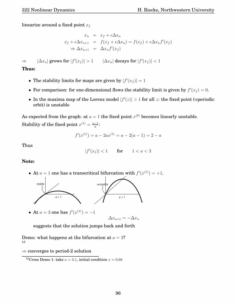
322 Nonlinear Dynamics H. Riecke, Northwestern University
linearize around a fixed point xf
xn = xf + ǫ∆xn
xf + ǫ∆xn+1 = f(xf + ǫ∆xn) = f(xf ) + ǫ∆xnf′(xf )
⇒ ∆xn+1 = ∆xnf′(xf )
⇒ |∆xn| grows for |f ′(xf )| > 1 |∆xn| decays for |f ′(xf )| < 1
Thus:
• The stability limits for maps are given by |f ′(xf )| = 1
• For comparison: for one-dimensional flows the stability limit is given by f ′(xf ) = 0.
• In the maxima map of the Lorenz model |f ′(z)| > 1 for all z: the fixed point (=periodic
orbit) is unstable
As expected from the graph: at a = 1 the fixed point x(0) becomes linearly unstable.
Stability of the fixed point x(1) = a−1a:
f ′(x(1)) = a− 2ax(1) = a− 2(a− 1) = 2− a
Thus
|f ′(x1)| < 1 for 1 < a < 3
Note:
• At a = 1 one has a transcritical bifurcation with f ′(x(1)) = +1.
a > 1
stable
a < 1
unstable
• At a = 3 one has f ′(x(1)) = −1∆xn+1 = −∆xn
suggests that the solution jumps back and forth
Demo: what happens at the bifurcation at a = 3?13
⇒ converges to period-2 solution
13Cross Demo 1: take a = 3.1, initial condition x = 0.68
96

322 Nonlinear Dynamics H. Riecke, Northwestern University
n
odd n
even n
1 2 3 4
xn
14
Determine period-2 solution:
Period 2: fixed point under second iterate of f(x)
xn+2 = f(xn+1) = f (f(xn)) ≡ f (2)(xn)
= axn+1(1− xn+1) = a (a xn(1− xn)) (1− a xn(1− xn))
Fixed point of f (2) : xn+2 = xnx(2) = f (2)(x(2))
Fixed points of the first iterate f(x) itself are also fixed points of the second iterate. There-
fore the fixed point condition can be factored as
−x(xa + 1− a)︸ ︷︷ ︸
known fixed points
(a2x2 − a(1 + a)x+ 1 + a) = 0
Thus one gets two new fixed points of the second iterate f (2)
x(2)1,2 =
1
2a
1 + a±√a2 − 2a− 3
They arise in a pitch-fork bifurcation and exist for a > 3. 15
The fixed points of f (2) correspond to a period-2 orbit alternating x(2)1 ↔ x
(2)2
0 0.2 0.4 0.6 0.8 1x
n
0
0.2
0.4
0.6
0.8
1
x n+1
14Demo: logmap.m for plotting xn as a function of n15Cross Demo: use second iterate to see pitch-fork bifurcation
97

322 Nonlinear Dynamics H. Riecke, Northwestern University
Stability of the period-2 orbit x(2)1,2: consider the stability of the fixed points of the second
iterate
x(2)1,2 +∆xn+2 = f
(
f(x(2)1,2 +∆xn)
)
∆xn+2 =d
dx(f (f(x)))
∣∣∣∣x(2)1,2
︸ ︷︷ ︸
λ
∆xn
λ = f ′(
f(x(2)1,2))
f ′(x(2)1,2)
With
f(x(2)1,2) = x
(2)2,1
we get
λ = f ′(
x(2)1
)
f ′(
x(2)2
)
= a2(
1− 2x(2)1
)(
1− 2x(2)2
)
= a2(
1− 2(
x(2)1 + x
(2)2
)
+ 4x(2)1 x
(2)2
)
= a2 − 2a (1 + a) + (1 + a)2 −(a2 − 2a− 3
)
= −a2 + 2a+ 4
The stability limits are given by
λ1 = +1 ⇒ a = 3
λ2 = −1 ⇒ a = 1 +√6 ≈ 3.4495
Notes:
• At a = 3 the fixed point of f (1)(x) undergoes a period-doubling bifurcation and the
eigenvalue of its linearization is λ(1) = −1. The eigenvalue of the linearization of
f (2)(x) at a = 3 is
λ(2) = 1 = f ′
f(x(1))︸ ︷︷ ︸
x(1)
f ′ (x(1))= λ(1)λ(1)
• For a = 1+√6 the fixed point of f (2) becomes unstable in a period-doubling bifurcation:
birth of a period-4 orbit.
16
16Demo: succcessive bifurcations, a = 0..4, a = 3.3..4zoom in with left mouse zoom out in stopped plot with mouse outside figure. Cross Demo 3
98

322 Nonlinear Dynamics H. Riecke, Northwestern University
d1
d2
d3x = 12X
a1 a2 a3 a4a
Period-Doubling Cascade:
• There is an infinite number of period-doubling bifurcations, which accumulate at
a∞ = 3.569945672 . . .
• With each bifurcation the period doubles: at a∞ the period is infinite and dynamics
are not periodic any more.
99

322 Nonlinear Dynamics H. Riecke, Northwestern University
• The distance between successive bifurcations becomes smaller with each bifurcation.
Their ratio approaches a fixed value
limn→∞
an − an−1
an+1 − an= δ = 4.6692016091029909...
The constant δ is called the Feigenbaum constant, after M. Feigenbaum who discov-
ered the scaling and showed that it is universal for all maps with a single maximum.
In terms of a∞ this scaling can be written as
an = a∞ + Ae−δ′n
with
δ =1− eδ
′
e−δ′ − 1= eδ
′
δ′ = 1.54098809542
• The width of the bifurcation also gets smaller in each bifurcation. The ratio of the
widths, measured when one branch intersects xm = 12, also approaches a fixed value
limn→∞
dndn+1
= α = −2.5029...
The minus sign indicates that successive bifurcations are on opposite sides of the mid
point xm = 12.
• The approach to fixed fixed ratios suggests self-similarity as a∞ is approached: zoom-
ing in yields a picture that looks essentially the same again, the same structures
repeat on smaller scales
• The self-similarity can be described with a renormalization theory. It shows that
period-doubling cascades in all maps with a quadratic maximum have the same uni-
versal behavior. i.e. they all have the same values of the Feigenbaum constant δ andof α.
Among the early experimental observations of the period-doubling cascade to chaos and
the measurement of the Feigenbaum constant were experiments on Rayleigh-Benard con-
vection of mercury [?]:
δ = 4.4± 0.1
100

322 Nonlinear Dynamics H. Riecke, Northwestern University
a)
b)
Figure 13: Period doubling cascade observed in convection of mercury with a horizontal
magnetic field. The arrow in b) marks the fundamental frequency in the power spectrum.
Period 32 is just about visible in b). [?, ?]
17
17Demo: logmap_scan.m amin=3.5, amax = ainf − .1e − 10, 106 points , a∞ = 3.569945672 . Self-similarity
zoom in a− ainf = O(10−6)
101

322 Nonlinear Dynamics H. Riecke, Northwestern University
Chaotic Dynamics:
For a > a∞ the dynamics are chaotic and exhibit sensitive dependence on initial conditions.
0 500 1000 1500 2000 2500 3000
0.4
0.5
0.6
0.7
0.8
0.9
1
0 500 1000 1500 2000 2500 30000.47
0.475
0.48
0.485
0.49
0.495
0.5
0.505
0.51
0.515
0 500 1000 1500 2000 2500 300010
−16
10−14
10−12
10−10
10−8
10−6
10−4
10−2
0 500 1000 1500 2000 2500 3000
0.4
0.5
0.6
0.7
0.8
0.9
1
0 500 1000 1500 2000 2500 30000.46
0.48
0.5
0.52
0.54
0.56
0.58
0.6
0 500 1000 1500 2000 2500 300010
−16
10−14
10−12
10−10
10−8
10−6
10−4
10−2
100
0 500 1000 1500 2000 2500 3000
0.4
0.5
0.6
0.7
0.8
0.9
1
0 500 1000 1500 2000 2500 3000
0.35
0.4
0.45
0.5
0.55
0.6
0.65
0.7
0 500 1000 1500 2000 2500 300010
−16
10−14
10−12
10−10
10−8
10−6
10−4
10−2
100
Figure 14: Sensitive dependence on initial conditions. Left panel: orbit for two slightly
different initial conditions, x0 = 0.5 (red) and x0 = 0.5 + 10−8 (blue). Middle panel: zoomed
in showing the orbits for every 8th iteration. Right panel: growth of the difference between
orbits. a) a = 3.569994: chaotic period-32 band with the period 32 still clearly visible. b)
a = 3.5753: close to the merging of the period-8 and period-4 band. c) a = 3.6: chaotic
period-2 band.
In analogy to the Lyapunov exponents for flows introduce Lyapunov exponents for maps
λ = limn→∞
lim∆x0→0
1
nln
∣∣∣∣
∆xn∆x0
∣∣∣∣
102

322 Nonlinear Dynamics H. Riecke, Northwestern University
Use
∆xn = f (n) (x0 +∆x0)− f (n) (x0)
=df (n)
dx
∣∣∣∣x0
∆x0 =n∏
j=1
f ′ (xj)∆x0
with
xj = f (j) (x0)
Thus
λ = limn→∞
1
nln
∣∣∣∣∣
n∏
j=1
f ′ (xj)
∣∣∣∣∣= lim
n→∞1
n
n∑
j=1
ln |f ′(xj)|
For a periodic orbit with period p we get
λ =1
pln
∣∣∣∣∣
p∏
j=1
f ′ (xj)
∣∣∣∣∣=
1
pln
∣∣∣∣∣
df (n)
dx
∣∣∣∣x0
∣∣∣∣∣
Superstable orbits:
Ifdf(n)(x)
dx= 0 then λ→ −∞: small perturbations of such orbits decay extremely fast.
Consider for simplicity a superstable fixed point xss
∆xn = f ′(xss)︸ ︷︷ ︸
0
∆xn−1 +1
2f ′′(xss)∆x
2n−1 +O
(∆x3n
)
=1
2f ′′(xss)
(1
2f ′′(xss)∆x
2n−2
)2
=1
2f ′(xss)
[
1
2f ′′(xss)
(1
2f ′′(xss)∆x
2n−3
)2]2
=
(1
2f ′′(xss)
)∑n−1j=0 2j
(∆x0)(2n) =
(1
2f ′′(xss)
)2n−1
(∆x0)(2n)
=
(1
2f ′′(xss)
)−1 (1
2f ′′(xss)∆x0
)(2n)
This decay is much faster than exponential. For comparison
∆xn+1
∆xn=
c for exponential decay to stable fixed point
∝ ∆xn for convergence to superstable fixed point
e.g.10−1 10−2 10−3 10−4 10−5 10−6 for exponential decay
10−1 10−2 10−4 10−8 10−16 10−32 decay at superstable fixed point
Note:
• when a periodic orbit first arises its Lyapunov exponent is f ′(x) = +1
• when a periodic orbit undergoes a period-doubling bifurcation f ′(x) = −1
103

322 Nonlinear Dynamics H. Riecke, Northwestern University
• between these two bifurcations f ′(x) has to go through 0, λ→ −∞:
the periodic orbit is superstable
• At the period-doubling bifurcations perturbations grow or decay very slowly→ it takes
a long time for the orbit to approach the attractor. Measuring the bifurcation points
precisely is therefore computationaly quite expensive. To characterize the period-
doubling cascade it is computationally more efficient to mark the superstable points
rather than the bifurcation points (cf. homework)
18
Origin of the sensitive dependence on initial conditions:
Consider a = 4:
Notes:
• The interval [0, 12] is stretched all the way to [0, 1]
• The interval [12, 1] is also stretched in length to [0, 1], but it is at the same time folded
back
• Separation of trajectories requires stretching and folding because the trajectories are
stretched and at the same time confined to a finite interval.
The stretching suggests a positive Lyapunov exponent. A very rough hand-waving guess
gives
∆xn+1 ∼ 2∆xn ∼ 2n+1∆x0
leading to
λ ∼ limn→∞
1
2ln 2n+1 → ln 2.
18Demo 4 by Cross: plot Lyapunov exponent
104

322 Nonlinear Dynamics H. Riecke, Northwestern University
For a = 4 one can actually give an explicit exact solution of the iteration for any initial
condition. Rewrite the iteration
xn+1 = 4xn(1− xn)
in terms of a new variable θn defined via
xn = sin2 θn xn+1 = sin2 θn+1.
Then
sin2 θn+1 = 4 sin2 θn (1− sin2 θn︸ ︷︷ ︸
cos2 θn
) =
= (2 sin θn cos θn)2 = sin2(2θn)
Thus, in terms of the variable θ the dynamics are simple
θn+1 = 2θn
⇒ θn = 2nθ0
xn = sin2 (2nθ0) = sin2 (2n arcsin√x0)
The analytical solution allows to compute the Lyapunov exponent exactly as well
λ = limn→∞
1
nln
∣∣∣∣∣
df (n)(x)
dx
∣∣∣∣x0
∣∣∣∣∣
= limn→∞
1
nln
∣∣∣∣∣2 sin (2nθ0) cos (2
nθ0) 2n d
dxarcsin
√x
∣∣∣∣x0
∣∣∣∣∣
= ln 2 + limn→∞
(1
nO(1)
)
= ln 2
‘Chaotic’ regime, periodic windows:
a = 3.825 → 3.85 → 3.86a = 3.83 → 3.8219
19transient points: 1024 points:256 (to capture periods up to 256) ; intermittency before window 3:
a=3.82841 and a=3.828415
105

322 Nonlinear Dynamics H. Riecke, Northwestern University
Periodic windows in the chaotic regime20
• Tangent bifurcation (saddle-node bifurcation) of f (3)(x) at 1 +√8 = 3.8284
A stable and an unstable fixed point of f (3)(x) are created, corresponding to a stable
and an unstable period-3 orbit.
• Just before the saddle-node bifurcation the ‘ghost’ of the period-3 orbit traps the orbit
for a long time ⇒ intermittent behvaior: long durations of near period-3 behavior,
which are interrrupted by chaotic excursions.
• The period-3 orbit also undergoes a period-doubling cascade.
• There are also windows with period 5, 7, 9, 11, etc. and each window has its own
period-doubling cascade.
20use logmap.m demo to show time series a = 3.828415 has long laminar regions a = 3.82837plot the function f (3) in the plot: use Cross Demo 1: set compose=3. plot cobweb diagram.
106

322 Nonlinear Dynamics H. Riecke, Northwestern University
0 500 1000 1500 2000 2500 3000 3500 4000 4500 50000.1
0.2
0.3
0.4
0.5
0.6
0.7
0.8
0.9
1
Figure 15: Intermittency for a = 3.82841 reflecting the ‘ghost’ of the period-3 orbit that is
created via a saddle-node biufrcation (tangent bifurcation) at slightly larger a.
4.3 Strange Attractors and Fractal Dimensions
In the Lorenz system and the logistic map we saw that in the chaotic regime the trajectories
converged onto a complicated set, a strange attractor.
We still need to define an attractor more precisely:
A set A is called an attractor if
1. A is an invariant set: any trajectory that starts in A remains in A for all times.
2. A attracts an open set of initial conditions: there exists an open set U containing Asuch that any trajectory starting in U converges to A for t→ ∞.
3. A is minimal, i.e. there is no proper subset of A that satisfies conditions 1 and 2.
Note:
• The largest open set U satisfying condition 2 is the basin of attraction of the attractor
A.
The attractors of the Lorenz system and the logistic map give the impression of a complex
geometry: they are strange attractors. How can we characterize their geometry?21
Consider yet another system since both the Lorenz system and the logistic map have draw-
backs
21Despite their striking geometric properties strange attractors are often defined via the property of sensi-
tive dependence on initial conditions.
107

322 Nonlinear Dynamics H. Riecke, Northwestern University
• Lorenz system is complicated since it is three-dimensional:
for chaotic flows this is the minimal dimension, however.
• The logistic map is not invertible, i.e. the dynamics cannot be run backwards in time.
Chaotic one-dimensional maps have to be non-invertible, since they need to include
stretching and folding. The folding introduces the non-invertibility.
Two-dimensional, invertible map: Henon map
xn+1 = yn + 1− ax2nyn+1 = bxn
The map can be thought of as composed of the following steps
1. stretch and fold a rectangle into a parabolic shape
x→ x y → y + 1− ax2
2. compress in the x-directionx→ bx y → y
3. reflection about the diagonal to orient the object again along the original rectangle
x→ y y → x
Figure 16: Henon map decomposed
4.
Notes:
• The Henon map is indeed invertible
xn =1
byn+1
yn = xn+1 − 1 + ax2n = xn+1 − 1 +a
by2n+1
108

322 Nonlinear Dynamics H. Riecke, Northwestern University
• The Henon map is dissipative
Consider infinitesimal area dx dy and its mapping under a variable transformation
(x, y) → (u(x, y), v(x, y))
from multi-variable integration we know that the rectangle with area dx dy is trans-
formed into a parallelogram with area |detJ| dx dy where J(x, y) is the Jacobian of the
variable transformation.
r2
1r
r'2
r'1
The area of the parallelogram generated by r′1 and r′2 is given by
|r′1 × r′2| = |r1xr2y − r1yr2x| =∣∣∣∣
∂u
∂x∆x
∂v
∂y∆y − ∂u
∂y∆y
∂v
∂x∆x
∣∣∣∣= |detJ|∆x∆y
An iteration of the Henon map can be thought of as a variable transformation ⇒ the
change in area in the phase plane is determined by |detJ|
detJ =
∣∣∣∣
−2axn 1b 0
∣∣∣∣= −b
Thus: for |b| < 1 the Henon map is dissipative everywhere in the phase plane.
109

322 Nonlinear Dynamics H. Riecke, Northwestern University
Figure 17: Self-similarity in the Henon map for a = 1.4 and b = 0.3. Axes
[xmin, xmax, ymin, ymax] are [0,1,0,1], [0.69,0.91,0.13,0.2], [0.77,0.80,0.16,0.17], and
[0.7829,0.7875,0.1629,0.1643].
The Henon attractor exhibits self-similarity: zooming into the upper three-layered sheet of
the three sheets reveals again three sheets comprised of 1, 2, and 3 sheets each. How do
we characterize such structures?
Consider the following construction of a set S that is somewhat similar to the cross section
of the Henon attractor
1. Take the interval [0,1]
2. cut out the middle third
3. from each remaining subinterval cut out the middle third
4. repeat step 3 ad infinitum
Note:
• the resulting set S is called the Cantor set after Georg Cantor, the developer of set
theory
110

322 Nonlinear Dynamics H. Riecke, Northwestern University
Question:
• how many pieces make up the set S?
• can one count them?
• what is its cardinality?
Countable and uncountable sets:
• a set is countable if there is a 1-to-1 correspondence between each of its elements and
the natural numbers
Examples
1. The rational numbers are countable
each rational number pqcan be represented as an element in a matrix Q
q\p 1 2 3 4 5 61 1
121
. . .2 1
222
32
. . .3 1
3. . .
4 14
. . .5 1
525
then count Q11 → Q21 → Q12 → Q31 → Q22 → Q13 → Q41 → . . .
2. The real numbers in [0, 1] are not countable
Cantor showed this by contradiction using his ‘diagonal argument’:
Assume the real numbers were countable. Then they could be listed in sequence
0.x11 x12 x13 . . .
0.x21 x22 x23 . . .
0.x31 x32 x33 . . .
0.x41 x42 x43 . . .
. . .
. . .
with xij ∈ R.
Consider now the number
0.x11 x22 x33 . . .
where xjj 6= xjj for all j. This number is clearly a realy number but it is not in the list
because it differs from each number in the list by at least one digit. The enumerated
list of numbers is therefore not complete.
111

322 Nonlinear Dynamics H. Riecke, Northwestern University
3. What is the cardinality of the Cantor set?
Use again Cantor’s diagonal argument as in the case of the real numbers: each piece
can be labeled by a number q ∈ 0, 1, 2 whose digit at the lth position states whether
at the lth level of the Cantor construction this piece ends up in the left, middle or right
third subdivision of the interval
All points in S are then given by a number whose digits are taken from 0, 2, sincethe middle piece is always taken out22.
If the Cantor set is countable then the elements can be listed,
x1 = x11 x12 x13 . . .
x2 = x21 x22 x23 . . .
x3 = x31 x32 x33 . . .
Again, the number x11 x22 x33 . . . is not contained in the list, but it is in S.Therefore S is not countable.
What is the total length (‘measure’) of the Cantor set S?In each step a third of the remaining length is removed:
Lj =2
3Lj−1 =
(2
3
)j
⇒ limj→∞
Lj = limj→∞
(2
3
)j
= 0
Thus, the Cantor set
• is uncountable (like the real numbers, but unlike the rationals)
• has zero measure (like the rational numbers, but unlike the real numbers)
Dimensions
As one goes down the levels the number of pieces in the Cantor set increases and diverges:
the number of pieces diverges as one increases the spatial resolution
Compare with the usual shapes:
Square:
• the square can be covered by 4 squares of half the linear dimension
• as the linear dimension of the pieces is reduced by a factor r the number m required
to construct the square increase by a factor m
m = rd with d =lnm
ln r
Apply this approach to the Cantor set:
• in each step the linear dimension of the pieces decreases by a factor of 3
22It is like a binary representation.
112

322 Nonlinear Dynamics H. Riecke, Northwestern University
• in each step the number of elements goes up by a factor of 2
d(sim)Cantor =
ln 2
ln 3≈ 0.63
Notes:
• this definition of the dimension relies on the self-similarity of the structure: similarity
dimension.
Example:
von Koch23 curve:
Recursive construction:
• replace each straight line segment of length l by 4 segments of length l/3
Similarity dimension:
• in each step linear dimension of the pieces decreases by a factor of 3
• in each step the number of pieces increases by a factor of 4
d(sim)Koch =
ln 4
ln 3≈ 1.26
For sets that are not self-similar generalize the procedure: cover the set with elements of
size ǫ where ǫ→ 0, i.e. reduce the linear dimension by a factor of r = 1ǫ,
d(box) = limǫ→0
lnN(ǫ)
ln(1ǫ
)
Note:
• This defines the box counting dimension.
Apply to the Cantor set:
At each level choose ǫ =(13
)n, then one needs 2n ‘boxes’ to cover the Cantor set
d(box) = limn→∞
ln 2n
ln 1
( 13)
n
= limn→∞
n ln 2
n ln 3=
ln 2
ln 3
Example: Attractor of the Henon map
23von Koch (1870–1924)
113

322 Nonlinear Dynamics H. Riecke, Northwestern University
Figure 18: Box dimension of Henon attractor for 500, 1,000, and 100,000 points. Left
panels; attractor with boxes, right panels: scaling of the number of boxes with the box size.
The box dimension does not depend on how many points of the trajectory are inside a given
box as long as there is at least one point.
Correlation Dimension:
For a given point r on the attractor determine the number of other points on the attractor
that fall within a ball of size ǫ of rNr(ǫ) ∝ ǫdr
114

322 Nonlinear Dynamics H. Riecke, Northwestern University
dr is the pointwise dimension of r.
The correlation dimension is obtained by averaging Nr(ǫ) over all (sufficiently many) r of
the attractor
C(ǫ) =1
NN∑
i=1
Nri(ǫ)
with N the number of attractor points r included in the average.
Expecting
C(ǫ) ∝ ǫdc
define
dc =d lnC(ǫ)
d ln (ǫ)
Figure 19: Correlation dimension for Henon map and Lorenz equations [?].
Note:
• Dynamics do enter correlation dimension: where are the points dense, where not, i.e.
where in phase space is the system more often?
• one can show dc ≤ dbbut usually dc ∼ db
Note:
• there are further dimensions along these lines:
whole spectrum of dimensions generated by weighing the probability of finding points
in a small ball with different powers
115

322 Nonlinear Dynamics H. Riecke, Northwestern University
Lyapunov Dimension:
Include dynamics explicitly in the definition of the dimension
Consider dimension of a box that neither grows nor shrinks under the dynamics.
Point attractor
any box with d ≥ 1 shrinks to a point: dL = 0
Periodic orbit
line segments along the attractor are transported along the orbit without volume change
(on average), but area covering the width of the attractor shrinks to a line: dL = 1
Growth of a ν-dimensional volume in phase space is given by the expansions in the ν direc-
tions
V (t) = L1eλ1t L2e
λ2t L3eλ3t . . . Lνe
λν t
for V = const. we needν∑
i=1
λi = 0
1 2
λ i
1 2
λ i
dimension
Σ
ν
ν
i=1
116

322 Nonlinear Dynamics H. Riecke, Northwestern University
Arrange eigenvalues in decreasing order: λi ≥ λi+1
Consider
f(n) =
n∑
i=1
λi
Interpolate linearly the zero of f(n):
f(dL) = 0 ≈ f(ν) +f(ν + 1)− f(ν)
ν + 1− ν(dL − ν) ⇒ dL = ν − f(ν)
f(ν + 1)− f(ν)
Thus, choose ν to satisfy∑ν
i=1 λi > 0 but∑ν+1
i=1 λi < 0. Then the Lyapunov dimension is
defined by
dL = ν +1
|λν+1|ν∑
i=1
λi
Note:
• dL gives a measure of how many degrees of freedom are ”active"
4.4 Experimental Data: Attractor Reconstruction and Poincare Sec-
tion
Experimentally, one typically cannot monitor all or even a large fraction of the relevant
dynamical variables. How can one obtain relevant information about the attractor?
Given only the time series for a single dynamical variable x(t) one can reconstruct a repre-
sentation of the attractor using time-delayed coordinates:
• plot x(t) vs x(t− τ),x(t− 2τ), ..., x(−Nτ) etc.
• estimate the dimension (e.g. correlation dimension) of the resulting attractor as a
function of the number N of delays
• if the dimension saturates above some value of N one has found a sufficient embed-
ding dimension for the attractor
Example: Lorenz system
117

322 Nonlinear Dynamics H. Riecke, Northwestern University
Figure 20: Reconstruction of the Lorenz attractor using delayed coordinates. a) τ = 1, b)τ = 10, c) τ = 20, d) τ = 100.
118

322 Nonlinear Dynamics H. Riecke, Northwestern University
Figure 21: Attractor reconstruction for the Belousov-Zhabotinsky reaction. The delay used
is indicated in each panel [?].
Note:
• The geometric shape of the attractor reconstruction depends on the delay τ . its di-
mension dimension does not.
• For very small τ the delayed variable x(t − τ) is strongly correlated with x(t) ⇒they
do not provide independent information about the attractor.
• For very large τ the two variables are completely uncorrelated: they do not provide
insight into the attractor
• Optimal delay at intermediate values: first minimum of the mutual information be-
tween the two variables [?]
119

322 Nonlinear Dynamics H. Riecke, Northwestern University
From the attractor one may be able to obtain a description in terms of a map on the Poincare
section, which generates a cross-section of the attractor:
For an attractor embedded in 3 dimensions mark all locations where the trajectory crosses
a two-dimensional manifold in one direction. If that cross-section can be parameterized
sufficiently well by a single variable one may obtain an iterated map for the dynamics.
a) b)
Figure 22: Belousov-Zhabotinsky rection. a) Poincare section (dashed line in upper panel)
yields a thin line (middle panel). The dynamics on that Poincare section is well captured
by an (almost) one-dimensional iterated map on that Poincare section. The unimodal map
suggests the appearance of a period-doubling cascade. The spectrum (b) shows a periodic
oscillation and a chaotic oscillation that still reflectes an approximate period 4 [?].
120