applied real options analysis
TRANSCRIPT

Applied Real Options AnalysisFor the Finance and Decision Professional
Dan Zoppo
SSZ Corpwww.sszcorp.com
August 25, 2021
Applied Real Options Analysis

Downloadable ModelsReal Options and More
Weblog at Freehold Financehttp://[email protected]
Applied Real Options Analysis

Outline
1 Introduction - Why Real Option Analysis?2 Basics of Real Options: Some Theory and Simple Examples3 LSM Algorithm4 Example model in Analytica
Applied Real Options Analysis

IntroductionWhy Real Options?
Project Management minimizes risks via managerial flexibilityTraditional Valuation does not include the value of flexibilityIntegrate project management with financial valuation
Applied Real Options Analysis
IntroductionReal Option Uses
ValuationPure Valuation - reportingInvestment Decisions
Optimal Controls and PoliciesDetermine optimal operating policies
Applied Real Options Analysis

What are Real Options
Definition (Eduardo S. Schwartz - UCLA)Real options are contingent decisions that provide the opportunityto make a decision after uncertainty unfolds.
Future actions in response to new information drive optionvalueFirms can be thought of as bundles of real optionsROA captures how businesses actually operate
Applied Real Options Analysis

Some Examples
Options to ExpandNetflix starting a movie studio
Option to SwitchEthanol Plants at the start of the pandemic in 2020mothballed plants or switched to producing hand sanitizer.
Option to LearnR&D in biotech, pharmaceuticals, semi-conductors, etc.
Option to waitDelay new store openings
Applied Real Options Analysis

Traditional Valuation Approach - DCF
Recall:
Static NPV =T∑
t=0ρtCt
Ct is the cash flow in period tρt = 1
(1+r)t is the discount factorT <∞ is the finite terminal time periodStatic NPV does not depend on actions
Applied Real Options Analysis

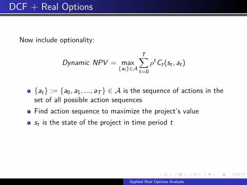
DCF + Real Options
Now include optionality:
Dynamic NPV = max{at}∈A
T∑t=0
ρtCt(st , at)
{at} := {a0, a1, ..., aT} ∈ A is the sequence of actions in theset of all possible action sequencesFind action sequence to maximize the project’s valuest is the state of the project in time period tCt(st , at) is the cash flow in period t and is now a function ofthe current state and the action taken
Applied Real Options Analysis

DCF + Real Options
Now include optionality:
Dynamic NPV = max{at}∈A
T∑t=0
ρtCt(st , at)
{at} := {a0, a1, ..., aT} ∈ A is the sequence of actions in theset of all possible action sequences
Find action sequence to maximize the project’s valuest is the state of the project in time period tCt(st , at) is the cash flow in period t and is now a function ofthe current state and the action taken
Applied Real Options Analysis

DCF + Real Options
Now include optionality:
Dynamic NPV = max{at}∈A
T∑t=0
ρtCt(st , at)
{at} := {a0, a1, ..., aT} ∈ A is the sequence of actions in theset of all possible action sequencesFind action sequence to maximize the project’s value
st is the state of the project in time period tCt(st , at) is the cash flow in period t and is now a function ofthe current state and the action taken
Applied Real Options Analysis
DCF + Real Options
Now include optionality:
Dynamic NPV = max{at}∈A
T∑t=0
ρtCt(st , at)
{at} := {a0, a1, ..., aT} ∈ A is the sequence of actions in theset of all possible action sequencesFind action sequence to maximize the project’s valuest is the state of the project in time period t
Ct(st , at) is the cash flow in period t and is now a function ofthe current state and the action taken
Applied Real Options Analysis

DCF + Real Options
Now include optionality:
Dynamic NPV = max{at}∈A
T∑t=0
ρtCt(st , at)
{at} := {a0, a1, ..., aT} ∈ A is the sequence of actions in theset of all possible action sequencesFind action sequence to maximize the project’s valuest is the state of the project in time period tCt(st , at) is the cash flow in period t and is now a function ofthe current state and the action taken
Applied Real Options Analysis

A Simple Example
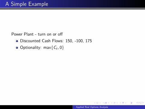
Power Plant - turn on or off
Discounted Cash Flows: 150, -100, 175Optionality: max{Ct , 0}static NPV = 150− 100 + 175 = 225Dynamic NPV = 150− 0 + 175 = 325Option Value = 325− 225 = 100
Applied Real Options Analysis

A Simple Example
Power Plant - turn on or offDiscounted Cash Flows: 150, -100, 175
Optionality: max{Ct , 0}static NPV = 150− 100 + 175 = 225Dynamic NPV = 150− 0 + 175 = 325Option Value = 325− 225 = 100
Applied Real Options Analysis
A Simple Example
Power Plant - turn on or offDiscounted Cash Flows: 150, -100, 175Optionality: max{Ct , 0}
static NPV = 150− 100 + 175 = 225Dynamic NPV = 150− 0 + 175 = 325Option Value = 325− 225 = 100
Applied Real Options Analysis

A Simple Example
Power Plant - turn on or offDiscounted Cash Flows: 150, -100, 175Optionality: max{Ct , 0}static NPV = 150− 100 + 175 = 225
Dynamic NPV = 150− 0 + 175 = 325Option Value = 325− 225 = 100
Applied Real Options Analysis

A Simple Example
Power Plant - turn on or offDiscounted Cash Flows: 150, -100, 175Optionality: max{Ct , 0}static NPV = 150− 100 + 175 = 225Dynamic NPV = 150− 0 + 175 = 325
Option Value = 325− 225 = 100
Applied Real Options Analysis

A Simple Example
Power Plant - turn on or offDiscounted Cash Flows: 150, -100, 175Optionality: max{Ct , 0}static NPV = 150− 100 + 175 = 225Dynamic NPV = 150− 0 + 175 = 325Option Value = 325− 225 = 100
Applied Real Options Analysis

The Two Types of Options
European OptionsSingle Exercise Point unaffected by other decisionsStrips of European options for multiple cash flow datesSimple and a good first approximation
American OptionsHave multiple exercise points - even continuousIntertemporal linkagesPath dependent constraints
Applied Real Options Analysis

The Two Types of Options
European Options
Single Exercise Point unaffected by other decisionsStrips of European options for multiple cash flow datesSimple and a good first approximation
American OptionsHave multiple exercise points - even continuousIntertemporal linkagesPath dependent constraints
Applied Real Options Analysis

The Two Types of Options
European OptionsSingle Exercise Point unaffected by other decisions
Strips of European options for multiple cash flow datesSimple and a good first approximation
American OptionsHave multiple exercise points - even continuousIntertemporal linkagesPath dependent constraints
Applied Real Options Analysis

The Two Types of Options
European OptionsSingle Exercise Point unaffected by other decisionsStrips of European options for multiple cash flow dates
Simple and a good first approximationAmerican Options
Have multiple exercise points - even continuousIntertemporal linkagesPath dependent constraints
Applied Real Options Analysis

The Two Types of Options
European OptionsSingle Exercise Point unaffected by other decisionsStrips of European options for multiple cash flow datesSimple and a good first approximation
American OptionsHave multiple exercise points - even continuousIntertemporal linkagesPath dependent constraints
Applied Real Options Analysis

The Two Types of Options
European OptionsSingle Exercise Point unaffected by other decisionsStrips of European options for multiple cash flow datesSimple and a good first approximation
American Options
Have multiple exercise points - even continuousIntertemporal linkagesPath dependent constraints
Applied Real Options Analysis

The Two Types of Options
European OptionsSingle Exercise Point unaffected by other decisionsStrips of European options for multiple cash flow datesSimple and a good first approximation
American OptionsHave multiple exercise points - even continuous
Intertemporal linkagesPath dependent constraints
Applied Real Options Analysis

The Two Types of Options
European OptionsSingle Exercise Point unaffected by other decisionsStrips of European options for multiple cash flow datesSimple and a good first approximation
American OptionsHave multiple exercise points - even continuousIntertemporal linkages
Path dependent constraints
Applied Real Options Analysis

The Two Types of Options
European OptionsSingle Exercise Point unaffected by other decisionsStrips of European options for multiple cash flow datesSimple and a good first approximation
American OptionsHave multiple exercise points - even continuousIntertemporal linkagesPath dependent constraints
Applied Real Options Analysis

How to Solve Real Option Models
Binomial Trees/LatticesPartial Differential Equations - Finite Difference MethodsRegression Monte Carlo
Applied Real Options Analysis

How to Structure American Options
Recall the sequence Problem:
V0(s0) = max{at}∈A
T∑t=0
ρtCt(st , at)
Transform it into a recursive problem:
V0(s0) = C0(s0, a0) +T∑
t=1ρtCt(st , at)
V0(s0) = C0(s0, a0) + ρV1(s1)
Applied Real Options Analysis

How to Structure American OptionsBellman Equation
Generalize previous slide and add uncertainty:
Vt(st) = maxat∈A(st)
(Ct(st , at) + ρE[Vt+1(st+1)|st ])
C(st , at) is current cash flow or contributionst+1 = f (st , at) is the state transition functionE[Vt+1(st+1)|st ] is the continuation valueE[Vt+1(st+1)|st ] = ?
Applied Real Options Analysis
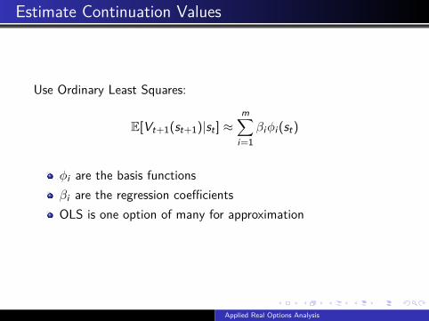
Estimate Continuation Values
Use Ordinary Least Squares:
E[Vt+1(st+1)|st ] ≈m∑
i=1βiφi (st)
φi are the basis functionsβi are the regression coefficientsOLS is one option of many for approximation
Applied Real Options Analysis

States
States can be decomposed into two types:1 Endogenous States
States that the action or decision will influenceE.g. modes of operations (Operating, suspended, mothballed,abandoned)
2 Exogenous StatesThe component of the state that is not influenced directly bythe decisionE.g. prices and costsUsually the stochastic variablesUncertainty plays a critical role
Applied Real Options Analysis

Putting it Together
LSM Algorithm
Applied Real Options Analysis
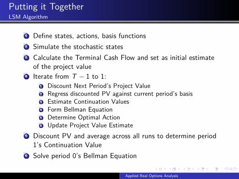
Putting it TogetherLSM Algorithm
1 Define states, actions, basis functions2 Simulate the stochastic states3 Calculate the Terminal Cash Flow and set as initial estimate
of the project value4 Iterate from T − 1 to 1:
1 Discount Next Period’s Project Value2 Regress discounted PV against current period’s basis3 Estimate Continuation Values4 Form Bellman Equation5 Determine Optimal Action6 Update Project Value Estimate
5 Discount PV and average across all runs to determine period1’s Continuation Value
6 Solve period 0’s Bellman Equation
Applied Real Options Analysis

Analytica LSM Algorithm
Applied Real Options Analysis