applied statistics comprehensive exam · based on a random sample of 3 colorado high school...
TRANSCRIPT

Applied Statistics Comprehensive Exam
August 2013
Ph.D Methods Exam
This comprehensive exam consists of 10 questions pertaining to methodological statisticaltopics.
1 This Ph.D level exam will run from 8:30 AM to 3:30 PM.
2 Please label each page with your identification number.
DO NOT USE YOUR NAME OR BEAR NUMBER.
3 Please write only on one side of each page.
4 Please leave one inch margins on all sides of each page.
5 Please number all pages consecutively.
6 Please label the day number (Day 1 or Day 2) on each page.
7 Please begin each question on a new page, and number each question.
8 Please do not staple pages together.
9 No wireless devices, formula sheets, or other outside materials are permitted.
10 Statistical tables and paper will be provided.
11 Relax and good luck!
I have read and understand the rules of this exam.
Signature: Date:

Applied Statistics and Research Methods - August 2013 - Methods Comprehensive 2
1.) Cancer rehabilitation researchers are interested in evaluating patients’ post-treatmentcardiopulmonary function using a continuous measure of “VO2 peak.” They would like tocompare this measure across four cancer stages (I, II, III, IV) while controlling for gender(female / male) and also patient age (measured in years). Researchers are not interested intesting hypotheses across gender and different ages, as it is accepted that cardiopulmonaryfunction differs for males and females and at different ages.
i. Describe an appropriate model that could be used to assess differences in cardiopul-monary function across cancer stages while accounting for gender and age.
ii. State the assumptions of your model.
iii. Your model must include an assumption about the relationship between age and lungcapacity. Describe how your model could be adjusted to change this assumption.
iv. Provide an interpretation of the intercept / constant term in your model. Is thismeaningful for making conclusions?
v. Provide an interpretation of the term(s) associated with cancer stage in your model.Give a detailed expression that could be used to test for the significance of this term,including the steps in the testing process, any calculations or formulas involved, andthe distribution of any test statistic(s) used.
2.) Higher education researchers are interested in trends of GPA for first-generation col-lege students during their first four semesters in college, and the corresponding effects ofmotivation and substance abuse. For their study they randomly selected 50 first-generationcollege students and initially classified their “motivation” level into one of three groups (low,medium, high). At the end of each of the first four semesters of school for each student,semester GPA is recorded as well as a self-reported continuous measure of “substance abuse.”
i. As a factor in a longitudinal panel study, how would you classify “motivation”?
ii. Clearly describe a model for GPA, accounting for all of the factors described.
iii. State the assumptions of your model. Specifically, what have you assumed about theeffect of “time”?
iv. Describe a process that could be used to test the effect of “motivation” on GPA.Include all steps in the testing process, any calculations or formulas involved, degreesof freedom and the distribution of any test statistic(s) used.
v. Assuming researchers are interested in assessing a “time trend” across the four semesters,describe in detail the types of trends that could be considered as well as how thesetrends could be assessed using your model.

Applied Statistics and Research Methods - August 2013 - Methods Comprehensive 3
3.) The following sample statistics were computed for a study of mercury contents in thewing muscles of Australian waterfowl. Calculate the 90% confidence interval for the contrastbelow assuming equal population variances.
C = µ3 − 12(µ1 + µ2)
Species N Mean SD
Shelduck 6 9 4Shoveler 3 10 5Blue-Billed 18 15 5
4.) Consider a Blocked One-Factor ANOVA model,
Yij = µ+ αi + bj + εij,
where i = 1, . . . , 4 indicates the four groups of interest, j = 1, . . . , 3 indicates the threeblocks, and εij ∼ N (0, σ2), independent.
i. Present the response vector Y and a full-rank design matrix X.
ii. Is µ+ α1 + b2 estimable? Justify your answer.
iii. Find an expression for the BLUE of µ+α1 + b2, and explain in what sense it is “best.”
iv. Find an expression for the variance of the BLUE of µ+ α1 + b2, and explain how thisvariance compares to the variance of other estimators of µ+ α1 + b2.
5.) An experiment was conducted in which 30 patients at an inpatient alcohol rehabilitationcenter were randomly assigned to receive one of three therapies. After three months oftreatment, two outcomes were measured using self-report questionnaires.
i. Write the one-way MANOVA model for this study in matrix form. Indicate the di-mensions of each matrix in your model.
ii. Describe the steps you would take to check the assumptions of this statistical analysis.

Applied Statistics and Research Methods - August 2013 - Methods Comprehensive 4
6.) Suppose we wish to study the effects of three factors on corn yields: amount of nitrogenadded, planting depth, and planting date. The nitrogen and depth factors each have twolevels, and the date factor has three levels. There are 24 plots available for this experiment:twelve are on a farm near Greeley, CO, and twelve are on a different farm near Brighton,CO.
i. Describe the experimental design you would use. Specifically describe the process forassigning treatments to EUs (plots). Briefly explain why you selected that design.
ii. Construct a partial ANOVA table that includes sources of variation, degrees of freedom,expected mean squares, and appropriate F-ratios.
7.) Given the data, use the Sign Test to test H0 : µ = 8.41 versus H1 : µ > 8.41.
8.30, 9.50, 9.60, 8.75, 8.40, 9.10, 9.25, 9.80, 10.05, 8.15, 10.00, 9.60, 9.80, 9.20, 9.30
8.) Compare and contrast stratified sampling to simple random sampling. What do thesedesigns have in common? How are they different? Give examples/applications of each design.Under what conditions is stratified sampling preferred over simple random sampling.
9.) The observations for delivery time, number of cases, and distance walked by the routerdrive were collected in four cities. A model was developed that relates delivery time y tocases x1, distance x2, and the city in which the delivery was made. Based on SAS outputon pages 5-7, answer the following questions.
i. Is there an indication that delivery site is an important variable?
ii. What conclusions can you draw regarding model adequacy?
10.) Based on a random sample of 3 Colorado high school classrooms, researchers haverecorded a measure of proficiency (proficient / not proficient) for a total of 93 students (31in the first classroom, 27 in the second, and 35 in the third). As proficiency is determinedby standardized exams, researchers would like to know if high school GPA is a reasonablepredictor of proficiency. They would also like to control for gender (male = 1 / female = 0)and block by class.
i. Based on researcher interest, construct an appropriate model for “proficiency.”
ii. Using the output on pages 8-10, assess the fit of this model.
iii. Using the output on pages 8-10, provide an interpretation for the coefficient for GPA,for gender, and also for the coefficient for the “class 2” indicator.
iv. Describe how your model would change if classes were treated as random blocks.

Applied Statistics and Research Methods - August 2013 - Methods Comprehensive 5

Applied Statistics and Research Methods - August 2013 - Methods Comprehensive 6

Applied Statistics and Research Methods - August 2013 - Methods Comprehensive 7

Applied Statistics and Research Methods - August 2013 - Methods Comprehensive 8
The LOGISTIC Procedure
Model Information
Data Set WORK.PROFICIENCY
Response Variable Proficiency
Number of Response Levels 2
Model binary logit
Optimization Technique Fisher’s scoring
Number of Observations Read 93
Number of Observations Used 93
Response Profile
Ordered Total
Value Proficiency Frequency
1 1 59
2 0 34
Probability modeled is Proficiency=1.
Model Convergence Status
Convergence criterion (GCONV=1E-8) satisfied.

Applied Statistics and Research Methods - August 2013 - Methods Comprehensive 9
Model Fit Statistics
Intercept
Intercept and
Criterion Only Covariates
AIC 124.122 85.754
SC 126.654 98.417
-2 Log L 122.122 75.754
Testing Global Null Hypothesis: BETA=0
Test Chi-Square DF Pr > ChiSq
Likelihood Ratio 46.3675 4 <.0001
Score 40.2811 4 <.0001
Wald 26.2467 4 <.0001
Analysis of Maximum Likelihood Estimates
Standard Wald
Parameter DF Estimate Error Chi-Square Pr > ChiSq
Intercept 1 -8.4772 1.8217 21.6537 <.0001
GPA 1 3.0771 0.6015 26.1689 <.0001
Gender 1 -0.0810 0.5912 0.0188 0.8910
Class2 1 -0.2019 0.7494 0.0726 0.7876
Class3 1 0.1339 0.6808 0.0387 0.8441
Odds Ratio Estimates
Point 95% Wald
Effect Estimate Confidence Limits
GPA 21.696 6.674 70.533
Gender 0.922 0.289 2.938
Class2 0.817 0.188 3.550
Class3 1.143 0.301 4.341

Applied Statistics and Research Methods - August 2013 - Methods Comprehensive 10
Partition for the Hosmer and Lemeshow Test
Proficiency = 1 Proficiency = 0
Group Total Observed Expected Observed Expected
1 9 1 0.69 8 8.31
2 9 1 1.43 8 7.57
3 9 3 2.85 6 6.15
4 9 4 4.50 5 4.50
5 9 7 6.31 2 2.69
6 9 8 7.08 1 1.92
7 9 7 7.84 2 1.16
8 9 8 8.21 1 0.79
9 10 9 9.42 1 0.58
10 11 11 10.66 0 0.34
Hosmer and Lemeshow Goodness-of-Fit Test
Chi-Square DF Pr > ChiSq
2.6864 8 0.9525

Applied Statistics Comprehensive Exam
August 2014
Ph.D Methods Exam
This comprehensive exam consists of 10 questions pertaining to methodological statisticaltopics.
1 This Ph.D level exam will run from 8:30 AM to 3:30 PM.
2 Please label each page with your identification number.
DO NOT USE YOUR NAME OR BEAR NUMBER.
3 Please write only on one side of each page.
4 Please leave one inch margins on all sides of each page.
5 Please number all pages consecutively.
6 Please label the day number (Day 1 or Day 2) on each page.
7 Please begin each question on a new page, and number each question.
8 Please do not staple pages together.
9 No wireless devices, formula sheets, or other outside materials are permitted.
10 Statistical tables and paper will be provided.
11 Relax and good luck!
I have read and understand the rules of this exam.
Signature: Date:

Applied Statistics and Research Methods - August 2014 - Methods Comprehensive 2
1.) Cancer rehabilitation researchers are interested in evaluating patients’ post-treatmentcardiopulmonary function using a continuous measure of “VO2 peak.” They would like tocompare this measure across four cancer stages (I, II, III, IV) while controlling for gender(female / male) and also patient age (measured in years). Researchers are not interested intesting hypotheses across gender and different ages, as it is accepted that cardiopulmonaryfunction differs for males and females and at different ages.
i. Describe an appropriate model that could be used to assess differences in cardiopul-monary function across cancer stages while accounting for gender and age.
ii. State the assumptions of your model.
iii. Your model must include an assumption about the relationship between age and lungcapacity. Describe how your model could be adjusted to change this assumption.
iv. Provide an interpretation of the intercept / constant term in your model. Is thismeaningful for making conclusions?
v. Provide an interpretation of the term(s) associated with cancer stage in your model.Give a detailed expression that could be used to test for the significance of this term,including the steps in the testing process, any calculations or formulas involved, andthe distribution of any test statistic(s) used.
2.) For each of the following three descriptions,
1. Determine the dependent and independent variables.
2. Determine which independent variable is nested within the other.
3. Sketch a representation of the data structure that makes the nesting clear. Do this inany way that makes sense to you!
i. Education researchers recorded the individual students’ standardized reading scores forfive classrooms selected from four different schools in a district. They are interested inthe effects of schools and of classrooms on these scores.
ii. A hospital is investigating basic supply expenditures. Three nurses are selected fromeach of four different floors and surveyed about supply usage once a month for a year.Nurses work only on a single floor. It is of interest to know the effect of the individualand also of the floor on average supply usage.
iii. Public health researchers are interested in rating residents on a “health index” scored ona scale from 1 to 100. Three states participated in their study, with three cities selectedfrom each state. Researchers recorded the health index value for five households in eachcity, and are interested in the effect of the state and the city on these values.

Applied Statistics and Research Methods - August 2014 - Methods Comprehensive 3
3.) Consider a 22 factorial design with two factors A and B. The levels of the factors may bearbitrarily called “low” and “high”. Consider the following data where an yield was recordedwhen the above mentioned factorial experiment was run in a completely randomized designwith three replicates.
Factor Replicate TotalA B Treatment Combination I II III− − A low, B low 28 25 27 80+ − A high, B low 36 32 32 100− + A low, B high 18 19 23 60+ + A high, B high 31 30 29 90
You may want to construct a standard order table (also known as Yates’ order) in orderto answer the following questions.
i. Obtain the estimates of main effects of A, B, and AB interaction.
ii. Obtain the sum of squares estimates SSA, SSB, and SSAB for A, B, and AB, respec-tively.
iii. The total corrected sum of squares for this experiment, SST is 323. Calculate the sumof squares for the error, SSE by subtracting SSA, SSB, and SSAB from the SST .
iv. Construct the analysis of variance table including the calculated F -statistic. Commenton the significance of the main effects and the interaction.
4.) Consider a Two-Factor ANOVA model:
Yijk = µ+ αi + βj + (αβ)ij + εijk,
where i = 1, 2, j = 1, 2, 3, and k = 1, 2.
i. Write the model in the form Y = Xβ + ε, giving Y, X, and β explicitly.
ii. Provide (but do not simplify!) an expression for the Least Squares Estimator β.
iii. Determine whether the linear expression βk − βl is estimable, for any combination kand l. What is the importance of identifying “estimable” functions?
iv. Describe how to find the Best Linear Unbiased Estimator for β1 − β2
β2 − β3
β3 − β1
.Explain in what sense the estimator is “best.”

Applied Statistics and Research Methods - August 2014 - Methods Comprehensive 4
5.) [This problem should be answered based on a 7-page SAS output on pages 7through 13.]
The admission officer of a graduate school has used an “index” of undergraduate GPAand graduate management aptitude test (GMAT) scores to help decide which applicantsshould be admitted to the graduate programs. The scatter plot of GPA vs GMAT (shown inthe attached SAS output) shows recent applicants who have been classified as “Admit (A)”,“Borderline (B)”, and “Reject (R)”.
A discriminant analysis and classification have been performed on the data and the resultsare shown in the attached SAS output. Answer the following questions. Note: when youanswer, make sure to include the associated statistics. For example, if you decide to rejecta null hypothesis, you should mention the value of the appropriate test statistic and thecorresponding p-value.
i. Is there significant association between admission status (admitted, rejected, border-line) and the scores on GPA and GMAT?
ii. If there is significant association, we would like to perform a discriminant analysis.How many discriminant functions (DF) are possible for the given problem?
iii. Comment on the significance of the discriminant function(s).
iv. What is the overall effect size for the discriminant analysis? Comment on the effectsize of each of the discriminant functions.
v. Write the classification functions corresponding to each discriminant function. Usethe classification function(s) for classifying an applicant as “Admit” or “Reject” or“Borderline” who has GPA = 3.7 and GMAT score = 650
vi. In the SAS output, both resubstitution summary and crossvalidation summary forclassification are provided. Comment on the error of misclassification based on theseoutput.
vii. Is there a reason to believe that the classification function produces noticeably highererror rate than what we would have obtained by chance alone? Would you use thediscriminant functions obtained from this analysis to classify an applicant to eitheradmit, reject, or borderline? Justify.

Applied Statistics and Research Methods - August 2014 - Methods Comprehensive 5
6.) Consider a one-fourth fraction of a 25 factorial design with factors A,B,C,D,E. Answerthe following questions:
i. Suppose that the design generators for this design are I = ACE, I = BCDE. Writethe complete defining relation for this design.
ii. Show the standard order table for this 25−2 design with the design generators givenabove.
iii. What is the resolution of this design? Justify.
iv. For a 25−2 design with design generators considered above, assuming all three-factorand higher-order interactions as negligible, write the alias structure of the main effectsA,B,C,D,E.
v. Demonstrate how would you estimate the “pure” or de-aliased effect of A from sucha design. You should show the procedure in detail including necessary “new” aliasstructures and a table showing how the de-aliasing of the effect of A can be obtained.
vi. Is it possible to have a better 25−2 design for this situation? Briefly explain.
7.) Given the data, use the Sign Test to test H0 : µ = 8.41 versus H1 : µ > 8.41.
8.30, 9.50, 9.60, 8.75, 8.40, 9.10, 9.25, 9.80, 10.05, 8.15, 10.00, 9.60, 9.80, 9.20, 9.30
8.) Compare and contrast adaptive cluster sampling to simple random sampling. What dothese designs have in common? How are they different? Give examples/applications of eachdesign.

Applied Statistics and Research Methods - August 2014 - Methods Comprehensive 6
9.) The Berkeley Guidance Study was a longitudinal monitoring of girls born in Berkeley,California between January 1928 and June 1929, and followed for at least 18 years. Thevariables are described as follows.
Variable DescriptionHT18 Age 18 height (cm)HT2 Age 2 height (cm)LG9 Age 9 leg circumference (cm)ST9 Age 9 strength (kg)WT9 Age 9 weight (kg)WT18 Age 18 weight (kg)
Use the SAS output on page 14 to answer the following questions.
i. Test for significance of regression for the relationship betweenHT18 andHT2, LG9, ST9,WT9and WT18.
ii. Assess multicollinearity in the model, and describe the results.
iii. Use the model with 5 regressors to find the prediction for x0 with the following values
HT2 LG9 ST9 WT9 WT1891.4 26.61 62 30.1 76.3
iv. Using the partial F test, determine the contribution of WT9 and WT18 to the model.Note F.05(2, 130) = 3.065.
10.) Health researchers are interested in explaining the likelihood of myocardial infarction(MI, “heart attack”) using professional attributes. For their study they randomly selected 75individuals between 55 and 65 years of age and recorded each individual’s annual income (inthousands of dollars), whether the individual has a college degree, and whether the individualhas experienced at least one MI within the last 10 years.
i. Describe an appropriate Generalized Linear Model for this research situation. Clearlyexplain each term in your systematic component.
ii. Using the output on pages 15 to 16, assess the fit of this model.
iii. Using the output on pages 15 to 16, provide an interpretation of the coefficient for“college degree.” Also provide an interpretation of the coefficient for “annual income.”
iv. The significance of each independent variable can be assessed using Wald Statistics.Briefly explain the process of a Wald hypothesis test.
v. Suppose the researchers also want to model the variation in MI (using a variancemultiplier). Thinking of the properties of variance, describe an appropriate GeneralizedLinear Model for modeling variance (assume the same independent variables as parti).

Applied Statistics and Research Methods - August 2014 - Methods Comprehensive 7
SAS Output for Question 5
1
gmat
300
400
500
600
700
gpa
2.1 2.2 2.3 2.4 2.5 2.6 2.7 2.8 2.9 3.0 3.1 3.2 3.3 3.4 3.5 3.6 3.7 3.8
admit Admit Reject BorderlineA A A R R R B B B
A
AA
A
A
A
A
A
A
A
AA
A
A
A
A
A
A
A
AA
AA
A
A
A
A
A
A
A
A
R
R
R
RR
RR
R
R
R
RR
R
RR
R
R
R
R
R
R
R
R
R
R
R
R R
BB
B
B
B
B
B
B
B
B
B
B
B
B
B
B B
B
B
B
B
B
B
B
B
B

Applied Statistics and Research Methods - August 2014 - Methods Comprehensive 8
SAS Output for Question 5
The SAS System
The DISCRIM Procedure
2
Total Sample Size 85 DF Total 84
Variables 2 DF Within Classes 82
Classes 3 DF Between Classes 2
Number of Observations Read 85
Number of Observations Used 85
Class Level Information
admit Variable Name Frequency Weight Proportion
Prior Probability
Admit Admit 31 31.0000 0.364706 0.333333
Borderline Borderline 26 26.0000 0.305882 0.333333
Reject Reject 28 28.0000 0.329412 0.333333
Pooled Covariance Matrix Information
Covariance Matrix Rank
Natural Log of the Determinant of the Covariance Matrix
2 4.85035

Applied Statistics and Research Methods - August 2014 - Methods Comprehensive 9
SAS Output for Question 5
The SAS System
The DISCRIM Procedure Canonical Discriminant Analysis
3
Generalized Squared Distance to admit
From admit Admit Borderline Reject
Admit 0 10.06344 31.28880
Borderline 10.06344 0 7.43364
Reject 31.28880 7.43364 0
Multivariate Statistics and F Approximations
S=2 M=-0.5 N=39.5
Statistic Value F Value Num DF Den DF Pr > F
Wilks' Lambda 0.12637661 73.43 4 162 <.0001
Pillai's Trace 1.00963002 41.80 4 164 <.0001
Hotelling-Lawley Trace 5.83665601 117.72 4 96.17 <.0001
Roy's Greatest Root 5.64604452 231.49 2 82 <.0001
NOTE: F Statistic for Roy's Greatest Root is an upper bound.
NOTE: F Statistic for Wilks' Lambda is exact.
Canonical
Correlation
Adjusted Canonical
Correlation
Approximate Standard
Error
Squared Canonical
Correlation
Eigenvalues of Inv(E)*H = CanRsq/(1-CanRsq)
Eigenvalue Difference Proportion Cumulative
1 0.921702 0.920516 0.016417 0.849535 5.6460 5.4554 0.9673 0.9673
2 0.400119 . 0.091641 0.160095 0.1906 0.0327 1.0000
Test of H0: The canonical correlations in the current row and all that follow are zero
Likelihood
Ratio Approximate
F Value Num DF Den DF Pr > F
1 0.12637661 73.43 4 162 <.0001
2 0.83990454 15.63 1 82 0.0002

Applied Statistics and Research Methods - August 2014 - Methods Comprehensive 10
SAS Output for Question 5
The SAS System
The DISCRIM Procedure Canonical Discriminant Analysis
4
Total Canonical Structure
Variable Can1 Can2
gpa 0.969922 -0.243416
gmat 0.662832 0.748768
Between Canonical Structure
Variable Can1 Can2
gpa 0.994118 -0.108305
gmat 0.897852 0.440298
Pooled Within Canonical Structure
Variable Can1 Can2
gpa 0.860161 -0.510023
gmat 0.350860 0.936428

Applied Statistics and Research Methods - August 2014 - Methods Comprehensive 11
SAS Output for Question 5
The SAS System
The DISCRIM Procedure
5
Total-Sample Standardized Canonical Coefficients
Variable Can1 Can2
gpa 2.148737595 -0.805087984
gmat 0.698531804 1.178084322
Pooled Within-Class Standardized Canonical Coefficients
Variable Can1 Can2
gpa 0.9512430832 -.3564113077
gmat 0.5180918168 0.8737695880
Raw Canonical Coefficients
Variable Can1 Can2
gpa 5.008766354 -1.876682204
gmat 0.008568593 0.014451060
Class Means on Canonical Variables
admit Can1 Can2
Admit 2.773788370 0.246102784
Borderline -0.271055133 -0.644045724
Reject -2.819285930 0.325571519
Linear Discriminant Function for admit
Variable Admit Borderline Reject
Constant -240.37168 -177.31575 -133.89892
gpa 106.24991 92.66953 78.08637
gmat 0.21218 0.17323 0.16541

Applied Statistics and Research Methods - August 2014 - Methods Comprehensive 12
SAS Output for Question 5
The SAS System
The DISCRIM Procedure Classification Summary for Calibration Data: WORK.GPA
Resubstitution Summary using Linear Discriminant Function
6
Number of Observations and Percent Classified into admit
From admit Admit Borderline Reject Total
Admit 27 87.10
4 12.90
0 0.00
31 100.00
Borderline 1 3.85
25 96.15
0 0.00
26 100.00
Reject 0 0.00
2 7.14
26 92.86
28 100.00
Total 28 32.94
31 36.47
26 30.59
85 100.00
Priors 0.33333
0.33333
0.33333
Error Count Estimates for admit
Admit Borderline Reject Total
Rate 0.1290 0.0385 0.0714 0.0796
Priors 0.3333 0.3333 0.3333

Applied Statistics and Research Methods - August 2014 - Methods Comprehensive 13
SAS Output for Question 5
The SAS System
The DISCRIM Procedure Classification Summary for Calibration Data: WORK.GPA
Cross-validation Summary using Linear Discriminant Function
7
Number of Observations and Percent Classified into admit
From admit Admit Borderline Reject Total
Admit 26 83.87
5 16.13
0 0.00
31 100.00
Borderline 1 3.85
24 92.31
1 3.85
26 100.00
Reject 0 0.00
2 7.14
26 92.86
28 100.00
Total 27 31.76
31 36.47
27 31.76
85 100.00
Priors 0.33333
0.33333
0.33333
Error Count Estimates for admit
Admit Borderline Reject Total
Rate 0.1613 0.0769 0.0714 0.1032
Priors 0.3333 0.3333 0.3333

Applied Statistics and Research Methods - August 2014 - Methods Comprehensive 14
SAS Output for Question 9
Berkeley data
The REG ProcedureModel: Ht18_5regressors
Dependent Variable: HT18 HT18
Berkeley data
The REG ProcedureModel: Ht18_5regressors
Dependent Variable: HT18 HT18
Number of Observations Read 136
Number of Observations Used 136
Analysis of Variance
Source DFSum of
SquaresMean
Square F Value Pr > F
Model 5 6619.20745 1323.84149 43.67 <.0001
Error 130 3940.64072 30.31262
Corrected Total 135 10560
Root MSE 5.50569 R-Square 0.6268
Dependent Mean 172.57868 Adj R-Sq 0.6125
Coeff Var 3.19025
Parameter Estimates
Variable Label DFParameter
EstimateStandard
Error t Value Pr > |t|VarianceInflation
Intercept Intercept 1 95.21271 16.09348 5.92 <.0001 0
HT2 HT2 1 0.92626 0.17012 5.44 <.0001 1.45551
LG9 LG9 1 -1.89219 0.49505 -3.82 0.0002 6.61156
ST9 ST9 1 0.15934 0.03663 4.35 <.0001 1.42637
WT9 WT9 1 0.21869 0.21919 1.00 0.3203 7.62382
WT18 WT18 1 0.48105 0.05527 8.70 <.0001 1.54992
Berkeley data
The REG ProcedureModel: Ht18_3regressors
Dependent Variable: HT18 HT18
Berkeley data
The REG ProcedureModel: Ht18_3regressors
Dependent Variable: HT18 HT18
Number of Observations Read 136
Number of Observations Used 136
Analysis of Variance
Source DFSum of
SquaresMean
Square F Value Pr > F
Model 3 4054.68423 1351.56141 27.43 <.0001
Error 132 6505.16393 49.28154
Corrected Total 135 10560
Root MSE 7.02008 R-Square 0.3840
Dependent Mean 172.57868 Adj R-Sq 0.3700
Coeff Var 4.06776
Parameter Estimates
Variable Label DFParameter
EstimateStandard
Error t Value Pr > |t|
Intercept Intercept 1 67.42450 16.62263 4.06 <.0001
HT2 HT2 1 1.23598 0.20826 5.93 <.0001
LG9 LG9 1 -0.57232 0.28929 -1.98 0.0500
ST9 ST9 1 0.19329 0.04629 4.18 <.0001

Applied Statistics and Research Methods - August 2014 - Methods Comprehensive 15
SAS Output for Question 10
'
The LOGISTIC Procedure
Model Information
Data Set WORK.MIDATA
Response Variable MI
Number of Response Levels 2
Model binary logit
Optimization Technique Fisher's scoring
Probability modeled is MI='1'.
Model Convergence Status
Convergence criterion (GCONV=1E-8) satisfied.
Model Fit Statistics
Criterion Intercept
Only
Intercept and
Covariates
AIC 101.106 86.535
SC 103.423 93.487
-2 Log L 99.106 80.535
Testing Global Null Hypothesis: BETA=0
Test Chi-Square DF Pr > ChiSq
Likelihood Ratio 18.5712 2 <.0001
Score 16.2263 2 0.0003
Wald 12.7642 2 0.0017
Analysis of Maximum Likelihood Estimates
Parameter DF Estimate Standard
Error Wald
Chi-Square Pr > ChiSq
Intercept 1 -15.0145 5.0909 8.6985 0.0032
Income 1 0.1504 0.0504 8.9175 0.0028
CollegeDegree 1 1.8937 1.1298 2.8092 0.0937

Applied Statistics and Research Methods - August 2014 - Methods Comprehensive 16
SAS Output for Question 10
'
The LOGISTIC Procedure
Odds Ratio Estimates
Effect Point
Estimate 95% Wald
Confidence Limits
Income 1.162 1.053 1.283
CollegeDegree 6.644 0.726 60.830
Association of Predicted Probabilities and Observed Responses
Percent Concordant 78.3 Somers' D 0.568
Percent Discordant 21.6 Gamma 0.568
Percent Tied 0.1 Tau-a 0.269
Pairs 1316 c 0.784
Partition for the Hosmer and Lemeshow Test
Group Total
MI = 1 MI = 0
Observed Expected Observed Expected
1 8 1 0.36 7 7.64
2 8 0 0.84 8 7.16
3 8 2 1.57 6 6.43
4 8 4 2.21 4 5.79
5 8 1 2.81 7 5.19
6 8 1 3.35 7 4.65
7 8 4 3.84 4 4.16
8 8 5 4.60 3 3.40
9 11 10 8.41 1 2.59
Hosmer and Lemeshow Goodness-of-Fit Test
Chi-Square DF Pr > ChiSq 10.2674 7 0.1739

Applied Statistics Comprehensive Exam
August 2015
Ph.D Methods Exam
This comprehensive exam consists of 10 questions pertaining to methodological statisticaltopics.
1 This Ph.D level exam will run from 8:30 AM to 3:30 PM.
2 Please label each page with your identification number.
DO NOT USE YOUR NAME OR BEAR NUMBER.
3 Please write only on one side of each page.
4 Please leave one inch margins on all sides of each page.
5 Please number all pages consecutively.
6 Please label the day number (Day 1 or Day 2) on each page.
7 Please begin each question on a new page, and number each question.
8 Please do not staple pages together.
9 No wireless devices, formula sheets, or other outside materials are permitted.
10 Statistical tables and paper will be provided.
11 Relax and good luck!
I have read and understand the rules of this exam.
Signature: Date:

Applied Statistics and Research Methods - August 2015 - Methods Comprehensive 2
1.) [This problem should be answered based on a 1-page SAS output that followsall questions, beginning on Page 7.]
A team of researchers is interested in determining whether two methods of hypnoticinduction, I and II, differ with respect to their effectiveness. They begin by randomlysorting 20 volunteer subjects into two independent groups of 10 subjects each, with theaim of administering Method I to one group and Method II to the other. Before either ofthe induction methods is administered, each subject is pre-measured on a standard indexof “primary suggestibility,” which is a variable known to be correlated with receptivity tohypnotic induction group. Use the SAS output to answer the following questions.
i) Identify the dependent and independent variables.
ii) Write an appropriate model for this scenario.
iii) Specify appropriate null and alternate hypotheses for testing the linear relationshipbetween the dependent variable and standard index of primary suggestibility. Reportvalues for the F-statistic, degrees of freedom, and p-value and state the conclusion ofthis test.
iv) Specify appropriate null and alternate hypotheses for testing the group effect. Reportthe values for the F-statistic, degrees of freedom, and p-value and state the conclusionof this test.
2.) For each of the following scenarios, write the null and alternative hypotheses, and thestatistical method and test statistic to be used.
i) The director of food services in a school district is considering the addition of newitems to the cafeteria menu. One of the new items is a green salad topped with stripsof grilled chicken breast. After tasting the salad, students in the district’s elementary,middle, and high schools are asked to indicate their preference by circling one of thefollowing options: (a) Add it to the menu, (b) Do not add it to the menu, and (c)No opinion. The director of food services analyzes the data to determine if there aredifferences in the numbers of students in the district’s elementary, middle, and highschools that chose each of the three response options.
ii) A statistics instructor at a liberal arts college has noticed that psychology and sociologystudents seem to have more positive attitudes toward statistics compared with historyand English students. The professor administers the Statistics Attitudes Inventory(SAI) scale to all students on the first day of the fall semester. The inventory containstwenty Likert-scale items with responses ranging from Strongly Disagree to StronglyAgree. The responses of psychology, sociology, English, and history students are thencompared to determine if there are significant differences in attitudes among the fourgroups of students.

Applied Statistics and Research Methods - August 2015 - Methods Comprehensive 3
Question 2, Continued
iii) Many school districts administer readiness tests to students upon kindergarten entry. Apublisher of a new kindergarten readiness test wants to convince potential users of thetest that it can accurately predict students’ academic performance in first grade. Thetest publisher offers to administer the readiness test, free of charge, to all kindergartenstudents in the district. After the test is administered, the readiness test score foreach student is recorded. At the end of first grade, all students are administered astandardized achievement test. The readiness test scores obtained a year earlier andthe scores on the standardized achievement test administered at the end of the firstgrade are studied to determine whether, as the readiness test publisher predicted, thereadiness test can serve as a good predictor of end-of-year achievement of first-gradestudents.
3.) Respond to the following.
i) Explain in non-technical terms the concept of analysis of variance (ANOVA), and writedown the fundamental ANOVA identity. (This question is not about the use of ANOVAfor testing several population means.)
ii) ANOVA is used to test for the equality of several treatments. In performing ANOVA,we compare mean squares for treatments (MSTreat) and mean squares for errors(MSErr). Technically, the expected value for MSTreat is the true population variance,σ2.
Explain in your words: How does the comparison of these two mean squares help ustesting for the treatment effects?
4.) Consider a Blocked One-Factor ANOVA model,
Yij = µ+ αi + bj + εij,
where i = 1, . . . , 3 indicates the three groups of interest, j = 1, . . . , 4 indicates the fourblocks, and εij ∼ N (0, σ2), independent.
i. Present the response vector Y, parameter vector β and a full-rank design matrix X.
ii. For what values of i and j is µ+ αi + bj estimable? Justify your answer.
iii. Find an expression for the BLUE of µ+α1 + b1, and explain in what sense it is “best.”
iv. Find an expression for the variance of the BLUE of µ+ α1 + b1, and explain how thisvariance compares to the variance of other estimators of µ+ α1 + b1.

Applied Statistics and Research Methods - August 2015 - Methods Comprehensive 4
5.) [This problem should be answered based on a 7-page SAS output that followsall questions, beginning on Page 8.]
The admissions officer of a graduate school has used an “index” of undergraduate GPAand graduate management aptitude test (GMAT) scores to help decide which applicantsshould be admitted to the graduate programs. The scatter plot of GPA vs GMAT (shown inthe attached SAS output) shows recent applicants who have been classified as “Admit (A)”,“Borderline (B)”, and “Reject (R)”.
A discriminant analysis and classification have been performed on the data and the resultsare shown in the attached SAS output. Answer the following questions. Note: when youanswer, make sure to include the associated statistics. For example, if you decide to rejecta null hypothesis, you should mention the value of the appropriate test statistic and thecorresponding p-value.
i) Is there significant association between admission status (admitted, rejected, border-line) and the scores on GPA and GMAT?
ii) If there is significant association, we would like to perform a discriminant analysis.How many discriminant functions (DF) are possible for the given problem?
iii) Comment on the significance of the discriminant function(s).
iv) What is the overall effect size for the discriminant analysis? Comment on the effectsize of each of the discriminant functions.
v) Write the classification functions corresponding to each discriminant function. Usethe classification function(s) for classifying an applicant as “Admit” or “Reject” or“Borderline” who has GPA = 3.7 and GMAT score = 650
vi) In the SAS output, both resubstitution summary and crossvalidation summary forclassification are provided. Comment on the error of misclassification based on theseoutput.
vii) Is there a reason to believe that the classification function produces noticeably highererror rate than what we would have obtained by chance alone? Would you use thediscriminant functions obtained from this analysis to classify an applicant to eitheradmit, reject, or borderline? Justify.

Applied Statistics and Research Methods - August 2015 - Methods Comprehensive 5
6.) [This problem should be answered based on a 14-page SAS output that followsall questions, beginning on Page 15.]
An experiment on the yield of three varieties of oats (factor A) and four different levelsof manure (factor B) was described by F. Yates in his 1935 paper Complex Experiments.The experimental area was divided into 6 blocks. Each of these was then subdivided into 3whole plots.
The varieties of oat were sown on the whole plots according to a randomized completeblock design (so that every variety appeared in every block exactly once). Each whole plotwas then divided into 4 split plots, and the levels of manure were applied to the split plotsaccording to a randomized complete block design (so that every level of B appeared in everywhole plot exactly once).
The design, after randomization, is shown in the Table below. The yield is measured inquarter pounds.
Table 1: Split-plot design and yields (in quarter lb) for the oat experiment.
Block Level of A Level of B (yield) Block Level of A Level of B (yield)1 2 3(156) 2(118) 2 2 2(109) 3(99)
1(140) 0(105) 0(63) 1(70)0 0(111) 1(130) 1 0(80) 2(94)
3(174) 2(157) 3(126) 1(82)1 0(117) 1(114) 0 1(90) 2(100)
2(161) 3(141) 3(116) 0(62)3 2 2(104) 0(70) 4 1 3(96) 0(60)
1(89) 3(117) 2(89) 1(102)0 3(122) 0(74) 0 2(112) 3(86)
1(89) 2(81) 0(68) 1(64)1 1(103) 0(64) 2 2(132) 3(124)
2(132) 3(133) 1(129) 0(89)5 1 1(108) 2(126) 6 0 2(118) 0(53)
3(149) 0(70) 3(113) 1(74)2 3(144) 1(124) 1 3(104) 2(86)
2(121) 0(96) 0(89) 1(82)0 0(61) 3(100) 2 0(97) 1(99)
1(91) 2(97) 2(119) 3(121)
i) Explain briefly why it is a split-plot design?
ii) List the whole plot and split-plot factors along with their levels and types. Is thereany or more factors that you would consider as random? Justify.
iii) Write down the statistical model that you consider appropriate for predicting yield anddefine all the terms in the model.
iv) Now, consider someone else has conducted an analysis of the data. Only the SASoutput is available. Use the results produced by SAS to create a table to show theexpected mean squares expressions.
v) Use the provided SAS output to draw conclusions.

Applied Statistics and Research Methods - August 2015 - Methods Comprehensive 6
7.) Given the data, use the Sign Test to test H0 : µ = 8.41 versus H1 : µ > 8.41.
8.30, 9.50, 9.60, 8.75, 8.40, 9.10, 9.25, 9.80, 10.05, 8.15, 10.00, 9.60, 9.80, 9.20, 9.30
8.) Compare and contrast stratified sampling to simple random sampling. What do thesedesigns have in common? How are they different? Give examples/applications of each design.Under what conditions is stratified sampling preferred over simple random sampling?
9.) [This problem should be answered based on a 1-page SAS output that followsall questions, beginning on Page 29.]
An investigator is interested in understanding the relationship, if any, between the houseselling price (price) and size of home in square feet (size), number of bedrooms (beds),number of bathrooms (baths), anual taxes (Taxes), and house condition (New), which takesthe values of new or not new. Data were collected for 100 houses sold in a large city. Use theSAS output provided to answer the following questions. In this output, IntNT representsthe interaction between Taxes and New.
i) Specify appropriate null and alternate hypotheses for testing the adequacy of the overallmodel and state the conclusion of this test.
ii) Do a group test for the effects of Taxes, New, and their interaction.
iii) Describe the differences between two models; the model with the interaction of Newand Taxes, and the model without this interaction.
iv) Test the partial effect of New in two models; the model with the interaction of Newand Taxes, and the model without this interaction.
v) What would you tell to the investigator for the effect of New?
10.) Consider an experiment intended to evaluate the relationships between the volume ofpatients who utilize local Urgent Care (UC) services and the properties of the different UClocations. To collect data, various research assistants are recruited to sit in different UCwaiting rooms and count the number of patients who enter; however, research assistantscannot be trusted to sit in waiting rooms for the same amounts of time. In addition, thenumber of staff and the age of each location is also recorded.
i) Clearly present a standard count regression model that could be used to model themean number of patients using staff and age as predictors. What are the assumptionsof your model?
ii) Assume the parameter estimate for “staff” is βs = 1.45. How would you interpret thisestimate?
iii) What is “overdispersion”? What are the consequences of ignoring overdispersion in acount regression model? Explain why overdispersion can be expected for this researchsituation.
iv) Clearly describe two options for accounting for overdispersion in these data (assumeyou have recorded a variable for “research assistant” that can be used to group theobservations). Compare your two options to each other.

Applied Statistics and Research Methods - August 2015 - Methods Comprehensive 7
SAS output for Question 1Q1Q1
The GLM Procedure
Class LevelInformation
Class Levels Values
method 2 I II
Number of Observations Read 20
Number of Observations Used 20
The GLM Procedure
Dependent Variable: effectiveness
Source DFSum of
Squares Mean Square F Value Pr > F
Model 2 763.2920226 381.6460113 44.54 <.0001
Error 17 145.6579774 8.5681163
Corrected Total 19 908.9500000
R-Square Coeff Var Root MSE effectiveness Mean
0.839751 18.82402 2.927134 15.55000
Source DF Type I SS Mean Square F Value Pr > F
primary_suggestibili 1 585.8772306 585.8772306 68.38 <.0001
method 1 177.4147921 177.4147921 20.71 0.0003
Source DF Type III SS Mean Square F Value Pr > F
primary_suggestibili 1 643.2420226 643.2420226 75.07 <.0001
method 1 177.4147921 177.4147921 20.71 0.0003

Applied Statistics and Research Methods - August 2015 - Methods Comprehensive 8
SAS output for question 5
1
gmat
300
400
500
600
700
gpa
2.1 2.2 2.3 2.4 2.5 2.6 2.7 2.8 2.9 3.0 3.1 3.2 3.3 3.4 3.5 3.6 3.7 3.8
admit Admit Reject BorderlineA A A R R R B B B
A
AA
A
A
A
A
A
A
A
AA
A
A
A
A
A
A
A
AA
AA
A
A
A
A
A
A
A
A
R
R
R
RR
RR
R
R
R
RR
R
RR
R
R
R
R
R
R
R
R
R
R
R
R R
BB
B
B
B
B
B
B
B
B
B
B
B
B
B
B B
B
B
B
B
B
B
B
B
B

Applied Statistics and Research Methods - August 2015 - Methods Comprehensive 9
The SAS System
The DISCRIM Procedure
2
Total Sample Size 85 DF Total 84
Variables 2 DF Within Classes 82
Classes 3 DF Between Classes 2
Number of Observations Read 85
Number of Observations Used 85
Class Level Information
admit Variable Name Frequency Weight Proportion
Prior Probability
Admit Admit 31 31.0000 0.364706 0.333333
Borderline Borderline 26 26.0000 0.305882 0.333333
Reject Reject 28 28.0000 0.329412 0.333333
Pooled Covariance Matrix Information
Covariance Matrix Rank
Natural Log of the Determinant of the Covariance Matrix
2 4.85035

Applied Statistics and Research Methods - August 2015 - Methods Comprehensive 10
The SAS System
The DISCRIM Procedure Canonical Discriminant Analysis
3
Generalized Squared Distance to admit
From admit Admit Borderline Reject
Admit 0 10.06344 31.28880
Borderline 10.06344 0 7.43364
Reject 31.28880 7.43364 0
Multivariate Statistics and F Approximations
S=2 M=-0.5 N=39.5
Statistic Value F Value Num DF Den DF Pr > F
Wilks' Lambda 0.12637661 73.43 4 162 <.0001
Pillai's Trace 1.00963002 41.80 4 164 <.0001
Hotelling-Lawley Trace 5.83665601 117.72 4 96.17 <.0001
Roy's Greatest Root 5.64604452 231.49 2 82 <.0001
NOTE: F Statistic for Roy's Greatest Root is an upper bound.
NOTE: F Statistic for Wilks' Lambda is exact.
Canonical
Correlation
Adjusted Canonical
Correlation
Approximate Standard
Error
Squared Canonical
Correlation
Eigenvalues of Inv(E)*H = CanRsq/(1-CanRsq)
Eigenvalue Difference Proportion Cumulative
1 0.921702 0.920516 0.016417 0.849535 5.6460 5.4554 0.9673 0.9673
2 0.400119 . 0.091641 0.160095 0.1906 0.0327 1.0000
Test of H0: The canonical correlations in the current row and all that follow are zero
Likelihood
Ratio Approximate
F Value Num DF Den DF Pr > F
1 0.12637661 73.43 4 162 <.0001
2 0.83990454 15.63 1 82 0.0002

Applied Statistics and Research Methods - August 2015 - Methods Comprehensive 11
The SAS System
The DISCRIM Procedure Canonical Discriminant Analysis
4
Total Canonical Structure
Variable Can1 Can2
gpa 0.969922 -0.243416
gmat 0.662832 0.748768
Between Canonical Structure
Variable Can1 Can2
gpa 0.994118 -0.108305
gmat 0.897852 0.440298
Pooled Within Canonical Structure
Variable Can1 Can2
gpa 0.860161 -0.510023
gmat 0.350860 0.936428

Applied Statistics and Research Methods - August 2015 - Methods Comprehensive 12
The SAS System
The DISCRIM Procedure
5
Total-Sample Standardized Canonical Coefficients
Variable Can1 Can2
gpa 2.148737595 -0.805087984
gmat 0.698531804 1.178084322
Pooled Within-Class Standardized Canonical Coefficients
Variable Can1 Can2
gpa 0.9512430832 -.3564113077
gmat 0.5180918168 0.8737695880
Raw Canonical Coefficients
Variable Can1 Can2
gpa 5.008766354 -1.876682204
gmat 0.008568593 0.014451060
Class Means on Canonical Variables
admit Can1 Can2
Admit 2.773788370 0.246102784
Borderline -0.271055133 -0.644045724
Reject -2.819285930 0.325571519
Linear Discriminant Function for admit
Variable Admit Borderline Reject
Constant -240.37168 -177.31575 -133.89892
gpa 106.24991 92.66953 78.08637
gmat 0.21218 0.17323 0.16541

Applied Statistics and Research Methods - August 2015 - Methods Comprehensive 13
The SAS System
The DISCRIM Procedure Classification Summary for Calibration Data: WORK.GPA
Resubstitution Summary using Linear Discriminant Function
6
Number of Observations and Percent Classified into admit
From admit Admit Borderline Reject Total
Admit 27 87.10
4 12.90
0 0.00
31 100.00
Borderline 1 3.85
25 96.15
0 0.00
26 100.00
Reject 0 0.00
2 7.14
26 92.86
28 100.00
Total 28 32.94
31 36.47
26 30.59
85 100.00
Priors 0.33333
0.33333
0.33333
Error Count Estimates for admit
Admit Borderline Reject Total
Rate 0.1290 0.0385 0.0714 0.0796
Priors 0.3333 0.3333 0.3333

Applied Statistics and Research Methods - August 2015 - Methods Comprehensive 14
The SAS System
The DISCRIM Procedure Classification Summary for Calibration Data: WORK.GPA
Cross-validation Summary using Linear Discriminant Function
7
Number of Observations and Percent Classified into admit
From admit Admit Borderline Reject Total
Admit 26 83.87
5 16.13
0 0.00
31 100.00
Borderline 1 3.85
24 92.31
1 3.85
26 100.00
Reject 0 0.00
2 7.14
26 92.86
28 100.00
Total 27 31.76
31 36.47
27 31.76
85 100.00
Priors 0.33333
0.33333
0.33333
Error Count Estimates for admit
Admit Borderline Reject Total
Rate 0.1613 0.0769 0.0714 0.1032
Priors 0.3333 0.3333 0.3333

Applied Statistics and Research Methods - August 2015 - Methods Comprehensive 15
SAS output for question 6
Oats Experiment Data
1
Obs block WP A B yield
1 1 1 2 3 156
2 1 1 2 1 140
3 1 1 2 2 118
4 1 1 2 0 105
5 1 2 0 0 111
6 1 2 0 3 174
7 1 2 0 1 130
8 1 2 0 2 157
9 1 3 1 0 117
10 1 3 1 2 161
11 1 3 1 1 114
12 1 3 1 3 141
13 2 1 2 2 109
14 2 1 2 0 63
15 2 1 2 3 99
16 2 1 2 1 70
17 2 2 1 0 80
18 2 2 1 3 126
19 2 2 1 2 94
20 2 2 1 1 82
21 2 3 0 1 90
22 2 3 0 3 116
23 2 3 0 2 100
24 2 3 0 0 62
25 3 1 2 2 104
26 3 1 2 1 89
27 3 1 2 0 70
28 3 1 2 3 117
29 3 2 0 3 122
30 3 2 0 1 89
31 3 2 0 0 74
32 3 2 0 2 81
33 3 3 1 1 103
34 3 3 1 2 132
35 3 3 1 0 64

Applied Statistics and Research Methods - August 2015 - Methods Comprehensive 16
Oats Experiment Data
2
Obs block WP A B yield
36 3 3 1 3 133
37 4 1 1 3 96
38 4 1 1 2 89
39 4 1 1 0 60
40 4 1 1 1 102
41 4 2 0 2 112
42 4 2 0 0 68
43 4 2 0 3 86
44 4 2 0 1 64
45 4 3 2 2 132
46 4 3 2 1 129
47 4 3 2 3 124
48 4 3 2 0 89
49 5 1 1 1 108
50 5 1 1 3 149
51 5 1 1 2 126
52 5 1 1 0 70
53 5 2 2 3 144
54 5 2 2 2 121
55 5 2 2 1 124
56 5 2 2 0 96
57 5 3 0 0 61
58 5 3 0 1 91
59 5 3 0 3 100
60 5 3 0 2 97
61 6 1 0 2 118
62 6 1 0 3 113
63 6 1 0 0 53
64 6 1 0 1 74
65 6 2 1 3 104
66 6 2 1 0 89
67 6 2 1 2 86
68 6 2 1 1 82
69 6 3 2 0 97
70 6 3 2 2 119

Applied Statistics and Research Methods - August 2015 - Methods Comprehensive 17
Oats Experiment Data
3
Obs block WP A B yield
71 6 3 2 1 99
72 6 3 2 3 121

Applied Statistics and Research Methods - August 2015 - Methods Comprehensive 18
4
The GLM Procedure
Class Level
Information
Class Levels Values
A 3 0 1 2
B 4 0 1 2 3
block 6 1 2 3 4 5 6
Number of Observations Read 72
Number of Observations Used 72
The GLM Procedure
Dependent Variable: yield
Source DF
Sum of
Squares Mean Square F Value Pr > F
Model 26 44017.19444 1692.96902 9.56 <.0001
Error 45 7968.75000 177.08333
Corrected Total 71 51985.94444
R-Square Coeff Var Root MSE yield Mean
0.846713 12.79887 13.30727 103.9722
Source DF Type I SS Mean Square F Value Pr > F
block 5 15875.27778 3175.05556 17.93 <.0001
A 2 1786.36111 893.18056 5.04 0.0106
A*block 10 6013.30556 601.33056 3.40 0.0023
B 3 20020.50000 6673.50000 37.69 <.0001
A*B 6 321.75000 53.62500 0.30 0.9322
Source DF Type III SS Mean Square F Value Pr > F
block 5 15875.27778 3175.05556 17.93 <.0001
A 2 1786.36111 893.18056 5.04 0.0106
A*block 10 6013.30556 601.33056 3.40 0.0023
B 3 20020.50000 6673.50000 37.69 <.0001
A*B 6 321.75000 53.62500 0.30 0.9322
The GLM Procedure

Applied Statistics and Research Methods - August 2015 - Methods Comprehensive 19
5
Source Type III Expected Mean Square
block Var(Error) + 4 Var(A*block) + 12 Var(block)
A Var(Error) + 4 Var(A*block) + Q(A,A*B)
A*block Var(Error) + 4 Var(A*block)
B Var(Error) + Q(B,A*B)
A*B Var(Error) + Q(A*B)
The GLM Procedure
Tests of Hypotheses for Mixed Model Analysis of Variance
Dependent Variable: yield
Source DF Type III SS Mean Square F Value Pr > F
block 5 15875 3175.055556 5.28 0.0124
* A 2 1786.361111 893.180556 1.49 0.2724
Error: MS(A*block) 10 6013.305556 601.330556
* This test assumes one or more other fixed effects are zero.
Source DF Type III SS Mean Square F Value Pr > F
A*block 10 6013.305556 601.330556 3.40 0.0023
* B 3 20021 6673.500000 37.69 <.0001
A*B 6 321.750000 53.625000 0.30 0.9322
Error: MS(Error) 45 7968.750000 177.083333
* This test assumes one or more other fixed effects are zero.
The GLM Procedure
Class Level
Information
Class Levels Values
A 3 0 1 2
B 4 0 1 2 3
block 6 1 2 3 4 5 6
Number of Observations Read 72
Number of Observations Used 72
The GLM Procedure

Applied Statistics and Research Methods - August 2015 - Methods Comprehensive 20
6
Dependent Variable: yield
Source DF
Sum of
Squares Mean Square F Value Pr > F
Model 26 44017.19444 1692.96902 9.56 <.0001
Error 45 7968.75000 177.08333
Corrected Total 71 51985.94444
R-Square Coeff Var Root MSE yield Mean
0.846713 12.79887 13.30727 103.9722
Source DF Type I SS Mean Square F Value Pr > F
block 5 15875.27778 3175.05556 17.93 <.0001
A 2 1786.36111 893.18056 5.04 0.0106
A*block 10 6013.30556 601.33056 3.40 0.0023
B 3 20020.50000 6673.50000 37.69 <.0001
A*B 6 321.75000 53.62500 0.30 0.9322
Source DF Type III SS Mean Square F Value Pr > F
block 5 15875.27778 3175.05556 17.93 <.0001
A 2 1786.36111 893.18056 5.04 0.0106
A*block 10 6013.30556 601.33056 3.40 0.0023
B 3 20020.50000 6673.50000 37.69 <.0001
A*B 6 321.75000 53.62500 0.30 0.9322
The GLM Procedure
Source Type III Expected Mean Square
block Var(Error) + 4 Var(A*block) + 12 Var(block)
A Var(Error) + 4 Var(A*block) + Q(A,A*B)
A*block Var(Error) + 4 Var(A*block)
B Var(Error) + Q(B,A*B)
A*B Var(Error) + Q(A*B)
The GLM Procedure
Tests of Hypotheses for Mixed Model Analysis of Variance
Dependent Variable: yield

Applied Statistics and Research Methods - August 2015 - Methods Comprehensive 21
7
Source DF Type III SS Mean Square F Value Pr > F
block 5 15875 3175.055556 5.28 0.0124
* A 2 1786.361111 893.180556 1.49 0.2724
Error: MS(A*block) 10 6013.305556 601.330556
* This test assumes one or more other fixed effects are zero.
Source DF Type III SS Mean Square F Value Pr > F
A*block 10 6013.305556 601.330556 3.40 0.0023
* B 3 20021 6673.500000 37.69 <.0001
A*B 6 321.750000 53.625000 0.30 0.9322
Error: MS(Error) 45 7968.750000 177.083333
* This test assumes one or more other fixed effects are zero.
50
75
100
125
150
175
yiel
d
0 1 2
A
Distribution of yield
Dunnett's t Tests for yield
Note: This test controls the Type I experimentwise error for comparisons of all treatments against a control.

Applied Statistics and Research Methods - August 2015 - Methods Comprehensive 22
8
Alpha 0.05
Error Degrees of Freedom 45
Error Mean Square 177.0833
Critical Value of Dunnett's t 2.28350
Minimum Significant Difference 8.772
Comparisons significant at the 0.05 level are
indicated by ***.
A
Comparison
Difference
Between
Means
Simultaneous
95%
Confidence
Limits
2 - 0 12.167 3.395 20.939 ***
1 - 0 6.875 -1.897 15.647
50
75
100
125
150
175
yiel
d
0 1 2 3
B
Distribution of yield
Dunnett's t Tests for yield

Applied Statistics and Research Methods - August 2015 - Methods Comprehensive 23
9
Note: This test controls the Type I experimentwise error for comparisons of all treatments against a control.
Alpha 0.05
Error Degrees of Freedom 45
Error Mean Square 177.0833
Critical Value of Dunnett's t 2.43088
Minimum Significant Difference 10.783
Comparisons significant at the 0.05 level are
indicated by ***.
B
Comparison
Difference
Between
Means
Simultaneous
95%
Confidence
Limits
3 - 0 44.000 33.217 54.783 ***
2 - 0 34.833 24.051 45.616 ***
1 - 0 19.500 8.717 30.283 ***

Applied Statistics and Research Methods - August 2015 - Methods Comprehensive 24
10
The Mixed Procedure
Model Information
Data Set WORK.OATS
Dependent Variable yield
Covariance Structure Variance Components
Estimation Method REML
Residual Variance Method Profile
Fixed Effects SE Method Model-Based
Degrees of Freedom Method Containment
Class Level
Information
Class Levels Values
A 3 0 1 2
B 4 0 1 2 3
block 6 1 2 3 4 5 6
Dimensions
Covariance Parameters 3
Columns in X 20
Columns in Z 24
Subjects 1
Max Obs per Subject 72
Number of Observations
Number of Observations Read 72
Number of Observations Used 72
Number of Observations Not Used 0
Iteration History
Iteration Evaluations -2 Res Log Like Criterion
0 1 564.36420957
1 1 529.02850701 0.00000000
Convergence criteria met.

Applied Statistics and Research Methods - August 2015 - Methods Comprehensive 25
11
Covariance
Parameter
Estimates
Cov Parm Estimate
block 214.48
A*block 106.06
Residual 177.08
Fit Statistics
-2 Res Log Likelihood 529.0
AIC (Smaller is Better) 535.0
AICC (Smaller is Better) 535.5
BIC (Smaller is Better) 534.4
Type 3 Tests of Fixed Effects
Effect
Num
DF
Den
DF F Value Pr > F
A 2 10 1.49 0.2724
B 3 45 37.69 <.0001
A*B 6 45 0.30 0.9322
Variance Components Estimation Procedure
Class Level
Information
Class Levels Values
A 3 0 1 2
B 4 0 1 2 3
block 6 1 2 3 4 5 6
Number of Observations Read 72
Number of Observations Used 72
MIVQUE(0) SSQ Matrix
Source block A*block Error yield
block 720.00000 240.00000 60.00000 190503.3
A*block 240.00000 240.00000 60.00000 87554.3
Error 60.00000 60.00000 60.00000 29857.3

Applied Statistics and Research Methods - August 2015 - Methods Comprehensive 26
12
MIVQUE(0) Estimates
Variance Component yield
Var(block) 214.47708
Var(A*block) 106.06181
Var(Error) 177.08333
The Mixed Procedure
Model Information
Data Set WORK.OATS
Dependent Variable yield
Covariance Structure Variance Components
Estimation Method REML
Residual Variance Method Profile
Fixed Effects SE Method Model-Based
Degrees of Freedom Method Containment
Class Level
Information
Class Levels Values
A 3 0 1 2
B 4 0 1 2 3
block 6 1 2 3 4 5 6
Dimensions
Covariance Parameters 3
Columns in X 20
Columns in Z 24
Subjects 1
Max Obs per Subject 72
Number of Observations
Number of Observations Read 72
Number of Observations Used 72
Number of Observations Not Used 0

Applied Statistics and Research Methods - August 2015 - Methods Comprehensive 27
13
Iteration History
Iteration Evaluations -2 Res Log Like Criterion
0 1 564.36420957
1 1 529.02850701 0.00000000
Convergence criteria met.
Covariance
Parameter
Estimates
Cov Parm Estimate
block 214.48
A*block 106.06
Residual 177.08
Fit Statistics
-2 Res Log Likelihood 529.0
AIC (Smaller is Better) 535.0
AICC (Smaller is Better) 535.5
BIC (Smaller is Better) 534.4
Type 3 Tests of Fixed Effects
Effect
Num
DF
Den
DF F Value Pr > F
A 2 10 1.49 0.2724
B 3 45 37.69 <.0001
A*B 6 45 0.30 0.9322
Least Squares Means
Effect A B Estimate
Standard
Error DF t Value Pr > |t|
A 0 97.6250 7.7975 10 12.52 <.0001
A 1 104.50 7.7975 10 13.40 <.0001
A 2 109.79 7.7975 10 14.08 <.0001
B 0 79.3889 7.1747 45 11.07 <.0001
B 1 98.8889 7.1747 45 13.78 <.0001
B 2 114.22 7.1747 45 15.92 <.0001
B 3 123.39 7.1747 45 17.20 <.0001
Applied Statistics and Research Methods - August 2015 - Methods Comprehensive 28
14
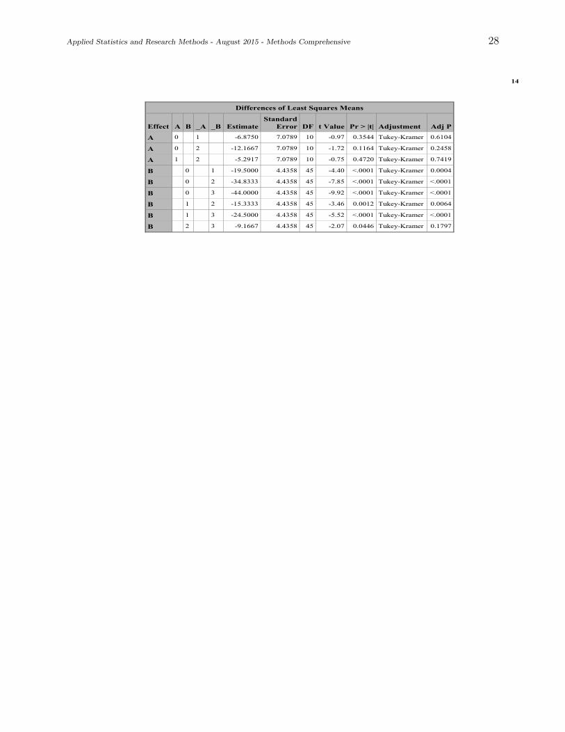
Differences of Least Squares Means
Effect A B _A _B Estimate
Standard
Error DF t Value Pr > |t| Adjustment Adj P
A 0 1 -6.8750 7.0789 10 -0.97 0.3544 Tukey-Kramer 0.6104
A 0 2 -12.1667 7.0789 10 -1.72 0.1164 Tukey-Kramer 0.2458
A 1 2 -5.2917 7.0789 10 -0.75 0.4720 Tukey-Kramer 0.7419
B 0 1 -19.5000 4.4358 45 -4.40 <.0001 Tukey-Kramer 0.0004
B 0 2 -34.8333 4.4358 45 -7.85 <.0001 Tukey-Kramer <.0001
B 0 3 -44.0000 4.4358 45 -9.92 <.0001 Tukey-Kramer <.0001
B 1 2 -15.3333 4.4358 45 -3.46 0.0012 Tukey-Kramer 0.0064
B 1 3 -24.5000 4.4358 45 -5.52 <.0001 Tukey-Kramer <.0001
B 2 3 -9.1667 4.4358 45 -2.07 0.0446 Tukey-Kramer 0.1797

Applied Statistics and Research Methods - August 2015 - Methods Comprehensive 29
SAS output for Question 9The SAS System
The REG ProcedureModel: MODEL1
Dependent Variable: Price
The SAS System
The REG ProcedureModel: MODEL1
Dependent Variable: Price
Number of Observations Read 100
Number of Observations Used 100
Analysis of Variance
Source DFSum of
SquaresMean
Square F Value Pr > F
Model 6 8.068673E11 1.344779E11 60.05 <.0001
Error 93 2.082822E11 2239593539
Corrected Total 99 1.01515E12
Root MSE 47324 R-Square 0.7948
Dependent Mean 155331 Adj R-Sq 0.7816
Coeff Var 30.46677
Parameter Estimates
Variable DFParameter
EstimateStandard
Error t Value Pr > |t|
Intercept 1 6868.82264 24689 0.28 0.7815
Size 1 66.42947 14.16148 4.69 <.0001
Beds 1 -10509 9178.44892 -1.14 0.2552
Baths 1 -2391.56172 11491 -0.21 0.8356
Taxes 1 37.50482 6.87171 5.46 <.0001
New 1 10796 41717 0.26 0.7964
IntNT 1 10.32976 12.74113 0.81 0.4196
The SAS System
The REG ProcedureModel: MODEL2
Dependent Variable: Price
The SAS System
The REG ProcedureModel: MODEL2
Dependent Variable: Price
Number of Observations Read 100
Number of Observations Used 100
Analysis of Variance
Source DFSum of
SquaresMean
Square F Value Pr > F
Model 3 7.117919E11 2.37264E11 75.08 <.0001
Error 96 3.033576E11 3159974854
Corrected Total 99 1.01515E12
Root MSE 56214 R-Square 0.7012
Dependent Mean 155331 Adj R-Sq 0.6918
Coeff Var 36.18959
Parameter Estimates
Variable DFParameter
EstimateStandard
Error t Value Pr > |t|
Intercept 1 -27290 28241 -0.97 0.3363
Size 1 130.43397 11.95115 10.91 <.0001
Beds 1 -14466 10583 -1.37 0.1749
Baths 1 6890.26655 13540 0.51 0.6120
The SAS System
The REG ProcedureModel: MODEL3
Dependent Variable: Price
The SAS System
The REG ProcedureModel: MODEL3
Dependent Variable: Price
Number of Observations Read 100
Number of Observations Used 100
Analysis of Variance
Source DFSum of
SquaresMean
Square F Value Pr > F
Model 5 8.053952E11 1.61079E11 72.19 <.0001
Error 94 2.097543E11 2231428577
Corrected Total 99 1.01515E12
Root MSE 47238 R-Square 0.7934
Dependent Mean 155331 Adj R-Sq 0.7824
Coeff Var 30.41119
Parameter Estimates
Variable DFParameter
EstimateStandard
Error t Value Pr > |t|
Intercept 1 4525.75265 24474 0.18 0.8537
Size 1 68.35009 13.93646 4.90 <.0001
Beds 1 -11259 9115.00315 -1.24 0.2198
Baths 1 -2114.37153 11465 -0.18 0.8541
Taxes 1 38.13524 6.81512 5.60 <.0001
New 1 41711 16887 2.47 0.0153

Applied Statistics Comprehensive Exam
August 2016
Ph.D Methods Exam
This comprehensive exam consists of 10 questions pertaining to methodological statisticaltopics.
1 This Ph.D level exam will run from 8:30 AM to 3:30 PM.
2 Please label each page with your identification number.
DO NOT USE YOUR NAME OR BEAR NUMBER.
3 Please write only on one side of each page.
4 Please leave one inch margins on all sides of each page.
5 Please number all pages consecutively.
6 Please label the day number (Day 1 or Day 2) on each page.
7 Please begin each question on a new page, and number each question.
8 Please do not staple pages together.
9 No wireless devices, formula sheets, or other outside materials are permitted.
10 Statistical tables and paper will be provided.
11 Relax and good luck!
I have read and understand the rules of this exam.
Signature: Date:

Applied Statistics and Research Methods - August 2016 - Methods Comprehensive 2
1.) A university health center tracks the number of flu-related visits during each monthof the fall semester. The center director wonders whether students come down with the flumore often around midterm (mid-October) and final (mid December) exams. Can these datashed any light on this issue?
Flu-Related Visits to the University Health Center(by months)
September October November December20 48 27 56
Is there any significant difference among the flu-related visits during the fall semester?Use an α level of .05 to test the appropriate hypothesis.
2.) In an exercise study, pulse gains (the difference in the post-exercise and pre-exercisepulse rates) were computed on forty persons. In this study, gender (female or male) andsmoking status (smoker or nonsmoker) for individuals were also registered. The summarydata is in the table below.
Group n mean VarianceMALE SMOKER 10 59.0 101.556FEMALE SMOKER 10 85.4 913.822MALE NONSMOKER 10 56.6 174.267FEMALE NONSMOKER 10 63.8 72.400
Consider the group (given in the table) as a four-level factor and answer the followingquestions.
i. Write down a contrast that compares
a) smokers and nonsmokers
b) female and male
c) female smokers and female nonsmokers
d) male smokers and male nonsmokers
ii. Estimate all the contrasts in part i.
iii. Find the MSE for the one-way ANOVA with the group as the only factor.
iv. Use the Bonferroni method to test all the comparisons in i. Consider αΣ = .05.

Applied Statistics and Research Methods - August 2016 - Methods Comprehensive 3
3.) An experiment concerned the evaluation of eight drugs (factor A at a = 8 levels) for thetreatment of arthritis. A second factor was the dose of the drug (factor B at b = 2 levels),and the third factor was the length of time (factor C at c = 2 levels) that a measurementwas taken after injection by a substance known to cause an inflammatory reaction.
The experimental unit used in the study were n = 64 rats. The response was theamount of fluid (in milliliter) measured in the pleural cavity of an animal after having beenadministered a particular treatment combination.
In pharmacological studies, time of the day has an effect on the response due to changinglaboratory conditions, etc. Consequently, the experiment was divided into blocks. It waspossible to make the blocks sizes to be 32, each set of 32 observations being measured on asingle day. Each treatment combination was measured once per day.
For the researcher, the effect of the drug (A) was of primary importance, and the effectsof B and C were of interest only in the form of an interaction with A.
Propose a design for this experiment and justify your opinion. Please provide sufficientdetails on the following items:
i. The justification of your choice of the design
ii. Clearly indicate how would the factors in this experiment be used (for example, whatfactor to be confounded, what factor or factors to be interacted with others, and soon.)
iii. Create a dummy data table putting factors in rows or columns as appropriate. Theresponse variable takes positive values between 5 and 15.
iv. Write the statistical model appropriate for your design and identify the model compo-nents.
v. Create the ANOVA table clearly showing the mean-squares expressions for each ofthem (i.e., the SS divided by appropriate denominator). You may use notations only,you do not have to write the actual mathematical expressions. You must show thecolumns such as the source of variation, df, SS, MS, and F.
4.) Consider the linear model defined in scalar notation by the following:
Yij = µi + β(xij − x..) + εij,
where i = 1, 2, 3, j = 1, 2, 3, 4, 5, and xT = [4, 2,−1, 0, 3, 5, 5, 8, 6, 8,−3,−4,−1, 0,−1]. (x.. =2.07)
i. Write the model in vector notation. Explicitly show Y, X, and β.
ii. Consider the hypothesis that all group means are equal, that is, H0 : µ1 = µ2, µ1 = µ3,and µ2 = µ3 (versus the alternative that at least one equality does not hold). Writethis hypothesis as a General Linear Hypothesis, explicitly showing CT and d.
iii. Determine whether the hypothesis from part ii is testable.
iv. Assuming testability, explain the process that could be followed to test H0.

Applied Statistics and Research Methods - August 2016 - Methods Comprehensive 4
5.) Respond to both parts of the question.
I. Briefly explain the concept of MANOVA understandable by someone with basic knowl-edge of ANOVA. When you answer this question, please address the following items.
i. Explanation of MANOVA and how does it relate to or differ from ANOVA?
ii. Name the test statistics to perform tests of significance in MANOVA.
iii. List the assumptions necessary to perform a MANOVA.
iv. Explain the concept of homogeneity of covariance matrices in the context ofMANOVA. Why it is important to check for this assumption? What test statisticwould you use for testing this assumption? If the p value for this test is 0.3001,what would be your conclusion abut this assumption?
II. Consider the following data. Provide some research questions that you would be able toanswer using ANOVA and MANOVA for this data set. State your null and alternativehypotheses both in writing and using statistical terms. Sketch the MANOVA tablerelated to your research question showing the sources of variation, the structure of thematrices of sum of squares within and sum of squares between, and degrees of freedomfor each items in the MANOVA table.
Gender Achievement ScoresMath Science Social Studies
Male 81 84 78Male 88 91 86Male 90 95 91Female 83 82 94Female 90 93 91Female 85 87 88

Applied Statistics and Research Methods - August 2016 - Methods Comprehensive 5
6.) An experiment was conducted to evaluate in which of five sound models the experimenterbest played a certain video game. The first three sound modes corresponded to three differenttypes of background music, as well as game sounds expected to enhance play. The fourthmode had game sounds but no background music. The fifth mode had no music or gamesounds. Denote these sound modes by the treatment factor levels 1-5, respectively.
The experimenter observed that the game required no warm up, that boredom and fatiguewould be a factor after 4 to 6 games, and that his performance varied considerably on a day-to-day basis. Hence, he used a Latin square design, with the two blocking factors being“day” and “time order of the game”.
The response measured was the game score, with higher scores being better. The designand resulting data are shown in the table below. The treatment factors are labeled 1-5 andthe response is within the parenthesis.
Day1 2 3 4 5
1 1 (94) 3 (100) 4 (98) 2 (101) 5 (112)Time 2 3 (103) 2 (11) 1 (51) 5 (110) 4 (90)Order 3 4 (114) 1 (75) 5 (94) 3 (85) 2 (100)
4 5 (100) 4 (74) 2 (70) 1 (93) 3 (106)5 2 (106) 5 (95) 3 (81) 4 (90) 1 (73)
Analyze the data and draw conclusions. In particular:
i. State the model and identify the model components.
ii. State the null and alternative hypothesis both in terms of statistical notation and inwriting.
iii. Analyze the data, create an ANOVA table.
iv. Draw conclusions.
7.) Discuss the differences between the Sign Test and Wilcoxons Signed Ranks Test. Includein your discussion the advantages / disadvantages of the two techniques.
8.) The Colorado Commission of Higher Education has recently hired you to estimate theaverage amount of scholarship money (in dollars) that each student receives per semester.Only state-supported universities/colleges in the state of Colorado are to be used. Privateschools are not to be included in the population for this study. What type of sampling designwould you use? Why? Explain, in detail, how you would obtain the data for your sample.What are the advantages/disadvantages of your design? What costs might be involved incollecting your data?

Applied Statistics and Research Methods - August 2016 - Methods Comprehensive 6
9.) In a study of faculty salaries in a small college in the Midwest, a linear regression modelwas fit, giving the fitted mean function,
E(Salary|Sex) = 24697− 3340× Sex,
where Sex equals one if the faculty member was female and zero if male. The response Salaryis measured in dollars.
i. Give a sentence that describes the meaning of the two estimated coefficients.
ii. An alternative mean function fit to these data with an additional term, Years, thenumber of years employed at this college, gives the estimated mean function,
E(Salary|Sex, Years) = 18065 + 201× Sex + 759× Years.
Now give a sentence that describes the meaning of the estimated coefficient of Sex.
iii. The important difference between these two mean functions is that the coefficient forSex has changed signs. Explain how this could happen.
10.) Health researchers are interested in modeling the likelihood of myocardial infarction(MI, “heart attack”) using professional attributes. For their study they randomly selected 75individuals between 55 and 65 years of age and recorded each individual’s annual income (inthousands of dollars), whether the individual has a college degree, and whether the individualhas experienced at least one MI within the last 10 years.
i. Describe some descriptive statistics that should be used to investigate the data (ta-bles, plots, etc.). What does each descriptive statistic tell you about the response orpredictors?
ii. Describe an appropriate statistical model that could be used to answer the researchinterests.
iii. Using the output on pages 7-8, assess the fit of the statistical model provided.
iv. Using the output on pages 7-8, provide interpretations of the effects of both incomeand college degree.
v. Assume researchers had instead gathered data on the number of heart attacks withinthe last ten years. Explain how your model from part ii would change to accommodatethis new response.

Applied Statistics and Research Methods - August 2016 - Methods Comprehensive 7
SAS Output for Question 10
'
The LOGISTIC Procedure
Model Information
Data Set WORK.MIDATA
Response Variable MI
Number of Response Levels 2
Model binary logit
Optimization Technique Fisher's scoring
Probability modeled is MI='1'.
Model Convergence Status
Convergence criterion (GCONV=1E-8) satisfied.
Model Fit Statistics
Criterion Intercept
Only
Intercept and
Covariates
AIC 101.106 86.535
SC 103.423 93.487
-2 Log L 99.106 80.535
Testing Global Null Hypothesis: BETA=0
Test Chi-Square DF Pr > ChiSq
Likelihood Ratio 18.5712 2 <.0001
Score 16.2263 2 0.0003
Wald 12.7642 2 0.0017
Analysis of Maximum Likelihood Estimates
Parameter DF Estimate Standard
Error Wald
Chi-Square Pr > ChiSq
Intercept 1 -15.0145 5.0909 8.6985 0.0032
Income 1 0.1504 0.0504 8.9175 0.0028
CollegeDegree 1 1.8937 1.1298 2.8092 0.0937

Applied Statistics and Research Methods - August 2016 - Methods Comprehensive 8
SAS Output for Question 10
'
The LOGISTIC Procedure
Odds Ratio Estimates
Effect Point
Estimate 95% Wald
Confidence Limits
Income 1.162 1.053 1.283
CollegeDegree 6.644 0.726 60.830
Association of Predicted Probabilities and Observed Responses
Percent Concordant 78.3 Somers' D 0.568
Percent Discordant 21.6 Gamma 0.568
Percent Tied 0.1 Tau-a 0.269
Pairs 1316 c 0.784
Partition for the Hosmer and Lemeshow Test
Group Total
MI = 1 MI = 0
Observed Expected Observed Expected
1 8 1 0.36 7 7.64
2 8 0 0.84 8 7.16
3 8 2 1.57 6 6.43
4 8 4 2.21 4 5.79
5 8 1 2.81 7 5.19
6 8 1 3.35 7 4.65
7 8 4 3.84 4 4.16
8 8 5 4.60 3 3.40
9 11 10 8.41 1 2.59
Hosmer and Lemeshow Goodness-of-Fit Test
Chi-Square DF Pr > ChiSq 10.2674 7 0.1739

Applied Statistics Comprehensive Exam
August 2017
Ph.D Methods Exam
This comprehensive exam consists of 10 questions pertaining to methodological statisticaltopics.
1 This Ph.D level exam will run from 8:30 AM to 3:30 PM.
2 Please label each page with your identification number.
DO NOT USE YOUR NAME OR BEAR NUMBER.
3 Please write only on one side of each page.
4 Please leave one inch margins on all sides of each page.
5 Please number all pages consecutively.
6 Please label the day number (Day 1 or Day 2) on each page.
7 Please begin each question on a new page, and number each question.
8 Please do not staple pages together.
9 No wireless devices, formula sheets, or other outside materials are permitted.
10 Statistical tables and paper will be provided.
11 Relax and good luck!
I have read and understand the rules of this exam.
Signature: Date:

Applied Statistics and Research Methods - August 2017 - Methods Comprehensive 2
1.) 502
2.) 502
3.) The effect of three different lubricating oils on fuel economy in diesel truck engines isbeing studied. (Fuel economy is measured using brake-specific fuel consumption after theengine has been running for 15 minutes.) Five different truck engines are available for thestudy. Experimenters have collected the following data.
TruckOil 1 2 3 4 51 0.500 0.634 0.487 0.329 0.5122 0.535 0.675 0.520 0.435 0.5403 0.513 0.595 0.488 0.400 0.510
i. Describe as completely as you can the type of design applied for this experiment. Whatare the advantages of using such a design?
ii. Present an appropriate model equation to describe how the two separate factors willbe analyzed.
iii. Provide an ANOVA table for this experiment. Include columns for source of varia-tion, sums of squares (you can show only the SS formulas in place of calculating thenumbers), degrees of freedom, mean squares (in terms of each SS ), and F-statistic.
iv. Assuming SSA = 0.0013 (Oil), SSB = 0.0307 (Truck), and SSE = 0.0710, perform atest of the significance of the Oil effect, and explain the result.
4.) 614
5.) 610
6.) Consider the Randomized Complete Block design, and the Latin Square design.
i. Describe each design in detail, providing notation for different factors and replicateswithin each design.
ii. Provide an outline of an ANOVA table for a specific case of each type of design,including only sources of variation and degrees of freedom.
iii. Discuss the relative advantages and disadvantages of each type of design with respectto the other.
7.) Given the data, use the Wilcoxon Signed Ranks Test to test:
H0 : µ = 107 versus H1 : µ 6= 107
99, 100, 90, 94, 135, 108, 107, 111, 119, 104, 127, 109, 117, 105, 125

Applied Statistics and Research Methods - August 2017 - Methods Comprehensive 3
8.) Compare and contrast stratified sampling to simple random sampling. What do thesedesigns have in common? How are they different? Give examples/applications of each design.Under what conditions is stratified sampling preferred over simple random sampling?

Applied Statistics and Research Methods - August 2017 - Methods Comprehensive 4
9.) 606
10.) Higher education researchers are interested in predicting the chances of first-generationstudents completing a four-year college degree within six years. Using historical records, theyhave retrieved the six-year completion status (graduated / not graduated) of approximately12,000 first-generation students from 520 undergraduate US institutions. They have alsorecorded each student’s gender (female / male), high school composite score (continuous),and parents’ income level at admission (in thousands of dollars).
i. Considering the interest of modeling six-year completion status, propose an appropriatemodel.
ii. Describe at least two descriptive statistics you would consult before applying yourmodel from part i. What are these descriptives used for?
iii. Describe at least three measures of fit that could be used to assess the adequacy ofyour model from part i.
iv. Specifically, discuss the Hosmer-Lemeshow fit statistic. How is it calculated? Howwould your perspective of this statistic change if the researchers had sampled 120,000students, instead of 12,000?
v. Specifically, discuss the Receiver Operating Characteristic (ROC) curve. How is itproduced, and how do you use the area under the curve to assess fit?
vi. Specifically, discuss the (studentized) deviance residuals. How are they used to assessfit?

Applied Statistics Comprehensive Exam
January 2013
Ph.D Methods Exam
This comprehensive exam consists of 10 questions pertaining to methodological statisticaltopics.
1 This Ph.D level exam will run from 8:30 AM to 3:30 PM.
2 Please label each page with your identification number.
DO NOT USE YOUR NAME OR BEAR NUMBER.
3 Please write only on one side of each page.
4 Please leave one inch margins on all sides of each page.
5 Please number all pages consecutively.
6 Please label the day number (Day 1 or Day 2) on each page.
7 Please begin each question on a new page, and number each question.
8 Please do not staple pages together.
9 No wireless devices, formula sheets, or other outside materials are permitted.
10 Statistical tables and paper will be provided.
11 Relax and good luck!
I have read and understand the rules of this exam.
Signature: Date:

Applied Statistics and Research Methods - January 2013 - Methods Comprehensive 2
1.) Teachers are often evaluated using measures of “growth” based on students’ standardizedexam scores. Administrators are interested in whether different grades show different levelsof typical growth. The following data present standardized measures of student growth for5 randomly selected teachers from each of grades 3, 4, 5, and 6.
Growth Scores
3rd Grade 4th Grade 5th Grade 6th Grade1 12.3 8.6 10.2 7.52 11.0 9.5 10.0 8.63 8.4 7.1 6.5 7.94 5.7 4.3 5.3 3.25 7.6 6.7 8.2 5.8Averages: 9.0 7.2 8.0 6.6
i. Construct an appropriate model that could be used to compare mean growth scoresacross grades. Include all assumptions for your model.
ii. Select one of your assumptions from i. Explain in detail how this assumption can betested, and describe one change you could make to your model if this assumption isnot met.
iii. Given SSE = 97.25, perform a test comparing growth across grades. Explain themeaning of the result using the language of student growth and grades.
Now suppose that teachers were randomly selected from 5 specific school districts (numbered1 through 5 in the table), such that one teacher is selected from each grade within eachdistrict.
iv. Explain how your model from i. would change to account for the possible clusteringwithin districts. Include all assumptions for your new model.
v. Explain in detail how the “no interaction” assumption can be assessed. Describe howyou would change your model from iv if this assumption is not met.

Applied Statistics and Research Methods - January 2013 - Methods Comprehensive 3
2.) Suppose the mean income (in thousands of dollars) for an individual is to be predictedusing years of education (from age 6), parents’ mean income, age of the individual (in years),residential tax rate (in percent), and high school GPA (on a 0 - 100 scale).
i. Construct an appropriate model for this research interest. Include all assumptions ofyour model.
ii. Explain how each assumption can be assessed. Describe how you would change yourmodel if the independence assumption fails due to cluster sampling.
iii. Describe what “multicollinearity” represents, and why it is a concern. Select variablesfrom this data situation that you think may cause problems with multicollinearity, andexplain why.
iv. Explain in detail at least two methods for detecting multicollinearity. Assuming youdetect multicollinearity in this data set, describe how you would proceed with yourmodel.
v. The following regression function is estimated.
ˆIncome = 9.63+1.2(Years of Ed)−0.3(Parents’ Income)+0.6(Age)+0.2(Tax Rate)−0.4(GPA)
Based on these parameter estimates, a colleague claims that “Years of Ed” is twice asimportant as “Age” and that higher “GPA” from high school tends to reduce futureincome. How would you respond to these statements?
3.) Consider a study in which high school basketball players are randomly assigned to one ofthree off-season training conditions: plyometric exercise for two months, weight-training fortwo months, or no extra training (control). Every players vertical leap ability is measuredweekly for two months. The primary goal is to test whether the treatments have differenteffects on change in players jumping ability.
i. Identify the name of the design used.
ii. Describe how you would analyse these data.
iii. Discuss how this analysis would differ from a basic analysis of variance and why suchmodifications are necessary.
iv. Identify all of the effects that would be testable. For each of those effects describewhat it means in practical language as if you were speaking to someone with minimalstatistical training.

Applied Statistics and Research Methods - January 2013 - Methods Comprehensive 4
4.) Consider a One-Factor ANOVA Cell Means Model,
Yij = µi + εij,
where i = 1, 2, 3, j = 1, . . . , 5, and
Y = [1 2 4 3 0 6 4 5 8 2 5 0 − 2 8 4]T .
i. Give the associated design matrix and parameter vector for this model.
ii. Consider performing pairwise comparisons between all combinations of group means.Present this as a General Linear Hypothesis of the form CTβ = d.
iii. Show that your General Linear Hypothesis is testable.
iv. Perform a test of your General Linear Hypothesis. (HINTS: (1) Here β will be groupaverages; (2) YT (I−P)Y = 94.0; (3) 2/5 −1/5 −1/5
−1/5 2/5 −1/5−1/5 −1/5 2/5
−
≈
1.1 −0.6 −0.6−0.6 1.1 −0.6−0.6 −0.6 1.1
.)
5.) Answer the following questions related to multivariate statistical methods.
i. Compare and contrast the use and purpose of predictive discriminant analysis vs.descriptive discriminant analysis.
ii. When discussing exploratory factor analysis, we often use the phrase “interpretablefactor solution.” Explain what this phrase means.
iii. Pretend you are working in the Research Consulting Lab. Use your imagination (donot use an example from SRM 610) to describe a research problem that a client mightbring for which you would advocate the use of MANOVA. Then describe how youwould convince them that MANOVA is the correct method.
6.) Experimental Design
i. Explain how a randomized complete block design with replication is different from atwo-factor completely randomized design.
ii. What is a Latin square design? What are the advantages of Latin square designs?What are the disadvantages?
iii. Why would an experimenter use a fractional factorial design? What are some draw-backs of using that design? Briefly describe how you would construct a quarter-fractiondesign for a study involving 6 factors each with 2 levels.

Applied Statistics and Research Methods - January 2013 - Methods Comprehensive 5
7.) Given the data, us the Sign Test to test H0 : µ = 8.41 vs H1 : µ > 8.41.
8.30, 9.50, 9.60, 8.75, 8.40, 9.10, 9.25, 9.80, 10.05, 8.15, 10.00, 9.60, 9.80, 9.20, 9.30
8.) Compare and contrast stratified random sampling to simple random sampling. What dothese designs have in common? How are they different? Give examples/applications of eachdesign.
9.) The SAS output gives a regression analysis of the systolic blood pressure (SBP), bodysize (QUET) a measure of size defined by QUET=100 (weight/height2), age (AGE), andsmoking history (SMK=0 if nonsmoker,SMK=1 if a current or previous smoker) for a hy-pothetical sample of 32 white males over 40 years old from the town of Angina. Note thatQUMK=QUET*SMK.
i. Determine a single multiple model that uses the data for both smokers and nonsmokersand that defines straight-line models for each group with possibly differing interceptsand slopes. Obtain the least-square line for smokers and nonsmokers by using thesingle multiple model.
ii. Test H0 : the two lines are parallel. State the appropriate null hypothesis in terms ofthe regression coefficients of the regression model.
iii. Suppose we fail to reject the null hypothesis in part (b) above. State the appropriateANACOVA regression model to use for comparing the mean blood pressure in the twosmoking categories, controlling for QUET.

Applied Statistics and Research Methods - January 2013 - Methods Comprehensive 6
10.) Consider the following data analysis, used to assess relationships between employmentstatus (employed, self-employed, unemployed) and race (White, Black, Latino) for bothmales and females.
i. Explain the differences between a Homogeneous Association model and a ConditionalIndependence model (employment status and race are assumed independent, condi-tional on gender).
ii. Using the SAS output, evaluate the Conditional Independence assumption.
iii. Using the Conditional Independence model, give the estimated odds ratio for employedversus self-employed.
Conditional Independence
The GENMOD Procedure
Criteria For Assessing Goodness Of Fit
Criterion DF Value Value/DF
Deviance 8 13.7980 1.7248
Scaled Deviance 8 13.7980 1.7248
Pearson Chi-Square 8 13.2196 1.6525
Scaled Pearson X2 8 13.2196 1.6525
Log Likelihood 2124.9958
Full Log Likelihood -55.2658
AIC (smaller is better) 130.5316
AICC (smaller is better) 161.9602
BIC (smaller is better) 139.4353
Algorithm converged.
Analysis Of Maximum Likelihood Parameter Estimates
Parameter DF Estimate Standard
Error
Wald 95%
Confidence
Limits
Wald
Chi-Square Pr > ChiSq
Intercept 1 3.7568 0.1160 3.5295 3.9842 1048.64 <.0001
Employment emp 1 0.0397 0.1065 -0.1690 0.2483 0.14 0.7095
Employment self 1 -1.3921 0.1704 -1.7261 -1.0581 66.74 <.0001
Race black 1 0.3986 0.1306 0.1427 0.6546 9.32 0.0023
Race latino 1 0.4389 0.1295 0.1850 0.6928 11.48 0.0007
Gender f 1 0.1013 0.1619 -0.2160 0.4186 0.39 0.5315
Employment*Gender emp f 1 0.1523 0.1570 -0.1554 0.4601 0.94 0.3320
Employment*Gender self f 1 0.2563 0.2430 -0.2200 0.7326 1.11 0.2916
Race*Gender black f 1 -0.4325 0.1844 -0.7940 -0.0711 5.50 0.0190
Race*Gender latino f 1 -0.5169 0.1847 -0.8789 -0.1548 7.83 0.0051
Scale 0 1.0000 0.0000 1.0000 1.0000
Note: The scale parameter was held fixed.

Applied Statistics and Research Methods - January 2013 - Methods Comprehensive 7
Homogeneous Association
The GENMOD Procedure
Criteria For Assessing Goodness Of Fit
Criterion DF Value Value/DF
Deviance 4 5.4046 1.3512
Scaled Deviance 4 5.4046 1.3512
Pearson Chi-Square 4 5.4024 1.3506
Scaled Pearson X2 4 5.4024 1.3506
Log Likelihood 2129.1925
Full Log Likelihood -51.0691
AIC (smaller is better) 130.1382
AICC (smaller is better) 270.1382
BIC (smaller is better) 142.6034
Algorithm converged.

Applied Statistics Comprehensive Exam
January 2014
Ph.D Methods Exam
This comprehensive exam consists of 10 questions pertaining to methodological statisticaltopics.
1 This Ph.D level exam will run from 8:30 AM to 3:30 PM.
2 Please label each page with your identification number.
DO NOT USE YOUR NAME OR BEAR NUMBER.
3 Please write only on one side of each page.
4 Please leave one inch margins on all sides of each page.
5 Please number all pages consecutively.
6 Please label the day number (Day 1 or Day 2) on each page.
7 Please begin each question on a new page, and number each question.
8 Please do not staple pages together.
9 No wireless devices, formula sheets, or other outside materials are permitted.
10 Statistical tables and paper will be provided.
11 Relax and good luck!
I have read and understand the rules of this exam.
Signature: Date:

Applied Statistics and Research Methods - January 2014 - Methods Comprehensive 2
1.) Briefly respond to the following.
i. Explain the difference(s) between “random” factors and “fixed” factors in an ANOVAmodel.
ii. Explain the difference of a between-subjects factor and a within-subjects factor.
iii. Explain the difference between crossed and nested factors.
2.) A pharmaceutical manufacturer wants to investigate the bioactivity of a new drug. Heconsiders three dosage levels of 20g, 30g and 40g and randomly assigns 4 subjects to eachdosage level. A response variable y was measured for each of 12 subjects.
i. Give an appropriate model for this research problem.
ii. Explain the meaning of the contrast ψ1 = µ1+µ3
2−µ2, where µi, i = 1, 2, 3 refers to the
mean of the measurement for the ith dosage level.
iii. Construct a contrast ψ2 that compares the means for the 20g dosage level and 40gdosage level and show that this contrast is orthogonal to ψ1.
iv. Given y1. = 29.75, y2. = 36.75, y3. = 44.75, and SSE = 288.25, perform a test of thesignificance of ψ1 at α = .05 level and explain the result. We know, 0.05t(11) = 1.80,
0.05t(10) = 1., 0.05t(9) = 1.83
3.) Respond to the following.
i. Explain in non-technical terms the concept of analysis of variance (ANOVA), and writedown the fundamental ANOVA identity. (This question is not about the use of ANOVAfor testing several population means.)
ii. ANOVA is used to test for the equality of several treatments. In performing ANOVA,we compare mean squares for treatments (MSTreat) and mean squares for errors(MSErr). Technically, expected value for MSTreat is the true population variance,σ2.
Explain in your words how does the comparison of these two mean squares help us intesting for the treatment effects.

Applied Statistics and Research Methods - January 2014 - Methods Comprehensive 3
4.) Consider an Additive Two-Factor ANOVA model:
Yijk = µ+ αi + βj + εijk,
where i = 1, 2, j = 1, 2, 3, and k = 1, 2, 3.
i. Construct an appropriate design matrix X for this model.
ii. Suppose it is of interest to test the hypothesis H0 : α1 = α2. Express this as a GeneralLinear Hypothesis.
iii. Construct a reduced model associated with H0 from part ii. Give the design matrix X0
for this reduced model.
iv. Using both design matrices, explicitly show how the hypothesis H0 can be evaluatedby comparing full and reduced models. Include an expression for the test statistic, thedistribution of your test statistic, along with degrees of freedom.
5.) The salmon fishery is a valuable resource for both the United States and Canada. Becauseit is a limited resource, it must be managed efficiently. Moreover, since more than onecountry is involved, problems must be solved equitably. To help regulate catches, samples offish taken during the harvest must be identified as coming from Alaskan or Canadian waters.The fish carry some information about their birth place in the growth rings on their scales.Typically, the rings associated with freshwater growth are smaller for the Alaskan-born thanfor the Canadian-born salmon.
The data set contains three variables measured on 100 specimens. The variables arecountry of origin (American or Canadian), freshwater growth ring size, and marine growthring size.
We perform a discriminant analysis using country of origin as the population into whichwe wish to classify the fish, and the variables freshwater and marine as the discriminators.Selected SAS output is provided on page 6.
i. Comment about overall significance of the discriminators in predicting country of ori-gin. Clearly mention what test statistic/statistics did you consider. How many dis-criminant functions would you obtain?
ii. Calculate overall effect size, effect size for the discriminant function and the effect sizesfor each of the discriminator (predictor) variables. In each case, explain what do theseeffect sizes mean in the context of this problem.
iii. Considering a linear discriminant function analysis, if you have a new measurementon a salmon fish with freshwater ring size = 90 and marine ring size = 420,would you classify it as American or Canadian? Justify your answer.

Applied Statistics and Research Methods - January 2014 - Methods Comprehensive 4
6.) The factors that influence longevity of AA-sized batteries are being studied. Threebrands of batteries (Premium, Average, Low) each with two types (regular, alkaline) will becompared.
i. Design an experiment to answer the research question. Give a scenario and identifyyour experimental units. What is the outcome variable and how would you measureit in your context? In particular, comment about the allocation of treatments to theexperimental units. Justify your selection of the design.
ii. Create a dummy data set that would be collected from such an experiment.
iii. Construct a partial ANOVA and show the sources of variation, appropriate degrees offreedoms, sum of squares, mean squares, and the F-statistic. Do not use the dummydata in ii to prepare the ANOVA table. How would you make conclusions from theexperiment?
7.) Given the data, use the Wilcoxon Signed Rank Test to test:
H0 : µ = 8.41 vs H1 : µ > 8.41.
8.30, 9.50, 9.60, 8.75, 8.40, 9.10, 9.25, 9.80, 10.05, 8.15, 10.00, 9.60, 9.80, 9.20, 9.30
8.) Compare and contrast simple random sampling to adaptive cluster sampling. What dothese designs have in common? How are they different? Give examples/applications of eachdesign.

Applied Statistics and Research Methods - January 2014 - Methods Comprehensive 5
9.) The Berkeley Guidance Study was a longitudinal monitoring of girls born in Berkeley,California between January 1928 and June 1929, and followed for at least 18 years. Thevariables are described as follows.
Variable DescriptionHT18 Age 18 height (cm)HT2 Age 2 height (cm)LG9 Age 9 leg circumference (cm)ST9 Age 9 strength (kg)WT9 Age 9 weight (kg)WT18 Age 18 weight (kg)
Use the SAS output on page 7 to answer the following questions.
i. Test for significance of regression for the relationship betweenHT18 andHT2, LG9, ST9,WT9and WT18.
ii. Assess multicollinearity in the model, and describe the results.
iii. Use the model with 5 regressors to find the prediction for x0 with the following values
HT2 LG9 ST9 WT9 WT1891.4 26.61 62 30.1 76.3
iv. Using the partial F test, determine the contribution of WT9 and WT18 to the model.Note F.05(2, 130) = 3.065.
10.) The National Medical Expenditure Survey (NMES) includes records that allow re-searchers to model “number of annual physician office visits” using “age” (in years), “gender”(an indicator for females) and “married” (indicator).
i. Using the output on pages 8-9, clearly describe an appropriate model for this researchsituation.
ii. Using the output on pages 8-9, evaluate the fit of the selected model.
iii. Provide interpretations of the parameter estimates for “age” and “married” in termsof the original problem.
iv. Suppose researchers have observed an excess of zeros in this type of data in the past(significantly more than expected). Describe in detail how your model could be ad-justed to account for this expectation.

Applied Statistics and Research Methods - January 2014 - Methods Comprehensive 6
SAS output for question 5
The SAS System
The DISCRIM Procedure
The SAS System
The DISCRIM Procedure
Total Sample Size 100 DF Total 99
Variables 2 DF Within Classes 98
Classes 2 DF Between Classes 1
Number of Observations Read 100
Number of Observations Used 100
Class Level Information
regionVariableName Frequency Weight Proportion
PriorProbability
A A 50 50.0000 0.500000 0.500000
C C 50 50.0000 0.500000 0.500000
Pooled Covariance MatrixInformation
CovarianceMatrix Rank
Natural Log of theDeterminant of theCovariance Matrix
2 12.72333

Applied Statistics and Research Methods - January 2014 - Methods Comprehensive 7
SAS output for question 9
Berkeley data
The REG ProcedureModel: Ht18_5regressors
Dependent Variable: HT18 HT18
Berkeley data
The REG ProcedureModel: Ht18_5regressors
Dependent Variable: HT18 HT18
Number of Observations Read 136
Number of Observations Used 136
Analysis of Variance
Source DFSum of
SquaresMean
Square F Value Pr > F
Model 5 6619.20745 1323.84149 43.67 <.0001
Error 130 3940.64072 30.31262
Corrected Total 135 10560
Root MSE 5.50569 R-Square 0.6268
Dependent Mean 172.57868 Adj R-Sq 0.6125
Coeff Var 3.19025
Parameter Estimates
Variable Label DFParameter
EstimateStandard
Error t Value Pr > |t|VarianceInflation
Intercept Intercept 1 95.21271 16.09348 5.92 <.0001 0
HT2 HT2 1 0.92626 0.17012 5.44 <.0001 1.45551
LG9 LG9 1 -1.89219 0.49505 -3.82 0.0002 6.61156
ST9 ST9 1 0.15934 0.03663 4.35 <.0001 1.42637
WT9 WT9 1 0.21869 0.21919 1.00 0.3203 7.62382
WT18 WT18 1 0.48105 0.05527 8.70 <.0001 1.54992
Berkeley data
The REG ProcedureModel: Ht18_3regressors
Dependent Variable: HT18 HT18
Berkeley data
The REG ProcedureModel: Ht18_3regressors
Dependent Variable: HT18 HT18
Number of Observations Read 136
Number of Observations Used 136
Analysis of Variance
Source DFSum of
SquaresMean
Square F Value Pr > F
Model 3 4054.68423 1351.56141 27.43 <.0001
Error 132 6505.16393 49.28154
Corrected Total 135 10560
Root MSE 7.02008 R-Square 0.3840
Dependent Mean 172.57868 Adj R-Sq 0.3700
Coeff Var 4.06776
Parameter Estimates
Variable Label DFParameter
EstimateStandard
Error t Value Pr > |t|
Intercept Intercept 1 67.42450 16.62263 4.06 <.0001
HT2 HT2 1 1.23598 0.20826 5.93 <.0001
LG9 LG9 1 -0.57232 0.28929 -1.98 0.0500
ST9 ST9 1 0.19329 0.04629 4.18 <.0001

Applied Statistics and Research Methods - January 2014 - Methods Comprehensive 8
SAS output for question 10
'
The UNIVARIATE Procedure Variable:
Visits
Moments
N 1200 Sum Weights 1200
Mean 21.125 Sum Observations 25350
Std Deviation 28.3835762 Variance 805.627398
Skewness 2.98654565 Kurtosis 14.2713188
Uncorrected SS 1501466 Corrected SS 965947.25
Coeff Variation 134.360124 Std Error Mean 0.81936327
Basic Statistical Measures
Location Variability
Mean 21.12500 Std Deviation 28.38358
Median 10.00000 Variance 805.62740
Mode 1.00000 Range 269.00000
Interquartile Range 26.00000

Applied Statistics and Research Methods - January 2014 - Methods Comprehensive 9
SAS output for question 10
'
The GENMOD Procedure
Model Information
Data Set WORK.VISITSDATA
Distribution Negative Binomial
Link Function Log
Dependent Variable Visits
Number of Observations Read 1200
Number of Observations Used 1200
Criteria For Assessing Goodness Of Fit
Criterion DF Value Value/DF
Deviance 1196 1276.6287 1.0674
Scaled Deviance 1196 1276.6287 1.0674
Pearson Chi-Square 1196 1246.1493 1.0419
Scaled Pearson X2 1196 1246.1493 1.0419
Log Likelihood 67083.4112
Full Log Likelihood -3911.5938
AIC (smaller is better) 7833.1876
AICC (smaller is better) 7833.2378
BIC (smaller is better) 7858.6380
Algorithm converged.
Analysis Of Maximum Likelihood Parameter Estimates
Parameter DF Estimate Standard
Error
Wald 95% Confidence
Limits Wald
Chi-Square Pr > ChiSq
Intercept 1 -1.2157 0.1556 -1.5208 -0.9106 61.01 <.0001
Age 1 0.0676 0.0026 0.0625 0.0727 672.64 <.0001
Female 1 -0.0204 0.0709 -0.1594 0.1186 0.08 0.7734
Married 1 0.0254 0.0650 -0.1021 0.1528 0.15 0.6967
Dispersion 1 0.2657 0.0147 0.2384 0.2962
Note: The negative binomial dispersion parameter was estimated by maximum likelihood.

Applied Statistics Comprehensive Exam
January 2015
Ph.D Methods Exam
This comprehensive exam consists of 10 questions pertaining to methodological statisticaltopics.
1 This Ph.D level exam will run from 8:30 AM to 3:30 PM.
2 Please label each page with your identification number.
DO NOT USE YOUR NAME OR BEAR NUMBER.
3 Please write only on one side of each page.
4 Please leave one inch margins on all sides of each page.
5 Please number all pages consecutively.
6 Please label the day number (Day 1 or Day 2) on each page.
7 Please begin each question on a new page, and number each question.
8 Please do not staple pages together.
9 No wireless devices, formula sheets, or other outside materials are permitted.
10 Statistical tables and paper will be provided.
11 Relax and good luck!
I have read and understand the rules of this exam.
Signature: Date:

Applied Statistics and Research Methods - January 2015 - Methods Comprehensive 2
1.) An experiment on sugar beets compared times and methods of applying mixed artificailfertilizers (NPK). The mean yields of sugar (cwt per acre) were as follows: no artificial,y1. = 38.7, artificial applied in January (plowed), y2 = 48.7, artificial applied in January(broadcast), y3 = 48.8, artificial applied in April (broadcast), y4 = 45.0.
i. Write down a contrast that compares January and April applications. Call this ψ1.
ii. Construct a contrast ψ2 that compares the means for artifact and no artifact. showthat this contrast is orthogonal to ψ1.
iii. If the experiment has three replications (n = 3 per treatment), and SSE = 62.51,perform a test of the significance of ψ1 at α = .05 level and explain the result. Weknow: 0.05t(14) = 1.761, 0.05t(15) = 1.753, 0.05t(16) = 1.745.
2.) Food scientists wish to study how urban and rural consumers rate cheddar cheeses forbitterness. Four 50-pound blocks of cheddar cheese of different types are obtained. Eachblock of cheese represents one of the segments of the market (for example, a sharp NewYork style cheese). The raters are students from a large introductory food science class. Tenstudents from rural backgrounds and ten students from urban backgrounds are selected atrandom from the pool of possible raters. Each rater will taste eight bites of cheese presentedin random order. The eight bites are two each from the four different cheeses, but the ratersdont know that. Each rater rates each bite for bitterness.
i. Describe the experimental design you would use.
ii. Specify the type of factors / independent variables, i.e within-subjects, between-subjects,nested, split-plot, whole plot, etc.
iii. Write down the model and clearly identify each term in your model and assumptionsof the model.
3.) An industrial engineer employed by a beverage bottler is interested in the effects of twodifferent types of 32-ounce bottles on the time to deliver 12-bottle cases of the product. Thetwo bottle types are glass and plastic. Two workers are used to perform a task consisting ofmoving 40 cases of the product 40 feet on a standard type of hand truck and stacking thecases in a display.
Four replicates of a 22 factorial design are performed, and the times observed are listedin the following table.
Suppose we denote the two factors as B for bottle type, and W for workers. Also thelevels of the factors may be arbitrarily called “low” and “high”. For instance, plastic maybe called “low” and glass may be called “high”. Similarly, worker 1 is considered “low” andworker 2 is considered “high”. Consider the following data where a yield was recorded whenthe above mentioned factorial experiment was run in a completely randomized design withfour replicates. (CONTINUED ON NEXT PAGE)

Applied Statistics and Research Methods - January 2015 - Methods Comprehensive 3
Factor ReplicateB-Bottle type W - Worker Treatment Combination I II III IV− − B low, W low 4.95 4.43 4.27 4.25+ − B high, W low 5.12 4.89 4.98 5.00− + B low, W high 5.28 4.91 4.75 4.71+ + B high, W high 6.65 6.24 5.49 5.55
You may want to construct a standard order table (also known as Yates’ order) in order toanswer the following questions.
i. Obtain the estimates of main effects of B, W , and the BW interaction.
ii. Obtain all sums of squares including the interaction effect and complete the ANOVAtable. Show the ANOVA table.
iii.) Write the appropriate hypotheses with regard to analyzing the above data. Commenton the significance of the main effects and the interaction effect.
4.) Consider the following general linear model, which represents a regression line thatchanges at the point X = X,
Yi = β0 + β1(Xi − X.) + β2Ii + β3(Ii × (Xi − X.)) + εi,
where Ii is an indicator that takes the value 1 if Xi > X and is 0 otherwise. Assume X = 30and the X-values observed are X = [12 15 26 31 39 42 48]T (so X. = 30.43).
i. Write the model in the form Y = Xβ + ε, giving X and β explicitly.
ii. Give interpretations of all model parameters.
iii. A reduced model with equal slopes on either side of X is proposed. Explicitly give thedesign matrix X0 and parameter vector β0 for this reduced model.
d. Explain how to test the significance of the difference in regression slopes on either sideof X. Include detaiivls such as the test statistic, distribution, and degrees of freedom.

Applied Statistics and Research Methods - January 2015 - Methods Comprehensive 4
5.) [This problem should be answered based on a 20-page SAS output beginningon page 7.]
Peanuts are an important crop in parts of the southern United States. In an effort todevelop improved plants, crop scientists routinely compare varieties with respect to severalvariables. The data for one two-factor experiment is available in the SAS output providedwith this exam.
Three varieties (5, 6, and 8) were grown at two geographical locations (location 1 and 2)and, in this case, the three variables representing yield and the two important grade-graincharacteristics were measured. The three variables are
Yield = Plot weightSdMtKer = Sound mature kernels (weight in grams–max of 250 grams)SeedSize = Seed size (weight, in grams, of 100 seeds)
The experiment was replicated twice.
i. Perform a two-factor MANOVA. Test for a location effect, a variety effect, and alocation-variety interaction effect. Use α = .05. Comment on the findings for each ofthe factors.
ii. List the MANOVA assumptions. In particular, comment on why the assumption ofhomogeneity of covariance matrices is important.
iii. Analyze the residuals from Part i. Do the usual MANOVA assumptions appear to besatisfied? Discuss.
iv. Using the results in part i, can we conclude that the location and/or variety effectsare additive? Additivity of effects means that a model without the interaction effectis good. If not, does the interaction effect show up for some (dependent) variables,but not for others? Check by using the three separate univariate two-factor ANOVAresults taking each DV at a time. Comment on your findings.
v. In the data, larger numbers correspond to better yield and grade-grain characteristics.Can we conclude that one variety is better than the other two for each characteristic(the DVs)? Discuss your answer using 95% Bonferroni simultaneous intervals for pairsof varieties.

Applied Statistics and Research Methods - January 2015 - Methods Comprehensive 5
6.) Consider a one-fourth fraction of a 25 factorial design with factors A,B,C,D,E. Answerthe following questions:
i. Suppose that the design generators for this design are I = ACE, I = BCDE. Writethe complete defining relation for this design.
ii. Show the standard order table for this 25−2 design with the design generators givenabove.
iii. What is the resolution of this design? Justify.
iv. For a 25−2 design with design generators considered above, assuming all three-factorand higher-order interactions as negligible, write the alias structure of the main effectsA,B,C,D,E.
v. Demonstrate how you would estimate the “pure” or de-aliased effect of A from sucha design. You should show the procedure in detail including necessary “new” aliasstructures and a table showing how the de-aliasing of the effect of A can be obtained.
vi. Is it possible to have a better 25−2 design for this situation? Briefly explain.
7.) Given the data, use the Sign Test to test H0 : µ = 8.41 vs h1 : µ > 8.41.
8.30, 9.50, 9.60, 8.75, 8.40, 9.10, 9.25, 9.80, 10.05, 8.15, 10.00, 9.60, 9.80, 9.20, 9.30
8.) The Colorado Commission of Higher Education has recently hired you to estimate theaverage amount of scholarship money (in dollars) that each student receives per semester.Only state-supported universities/colleges in the state of Colorado are to be used. Privateschools are not to be included in the population for this study. What type of sampling designwould you use? Why? Explain, in detail, how you would obtain the data for your sample.What are the advantages/disadvantages of your design? What costs might be involved incollecting your data?

Applied Statistics and Research Methods - January 2015 - Methods Comprehensive 6
9.) Explain what multicollinearity is. What are the sources and effects of multicollinearity?
10.) Higher education researchers are interested in predicting current high school students’chances of completing various levels of education, using parents’ income (in thousands ofdollars per year), gender (female, male), and race (African-American, Caucasian, Hispanic/ Latino) as predictors. The researchers conducted a retrospective study in which 20 highschool graduates over the age of 35 were randomly selected from each of the six combinationsof gender and race (giving 120 total subjects). Each subject was asked to estimate his/herparents’ annual income and to indicate whether he/she has completed high school, hascompleted an associate’s degree, has completed a bachelor’s degree, or has completed agraduate degree.
i. Propose an appropriate Generalized Linear Model (GLM) to predict the chances ofreaching each level of education. Clearly explain the meaning of each component andeach parameter included in your model.
ii. Compare your proposed model from part i with at least one other possible model usinga different link function.
iii. Assuming all 120 subjects provide different values for “parents’ income,” calculate the“error” degrees of freedom for your model.
iv. Explain the meaning of the “proportional odds assumption.” Does your model includesuch an assumption?
v. Suppose a single parameter for “parents’ income” is estimated to be β ≈ 0.35. Providean interpretation of this parameter estimate.

Applied Statistics and Research Methods - January 2015 - Methods Comprehensive 7
SAS output for question 5
Peanuts Data 1Peanuts Data 1
Obs location variety yield SdMtKer SeedSize
1 1 5 195.3 153.1 51.4
2 1 5 194.3 167.7 53.7
3 2 5 189.7 139.5 55.5
4 2 5 180.4 121.1 44.4
5 1 6 203.0 156.8 49.8
6 1 6 195.9 166.0 45.8
7 2 6 202.7 166.1 60.4
8 2 6 197.6 161.8 54.1
9 1 8 193.5 164.5 57.8
10 1 8 187.0 165.1 58.6
11 2 8 201.5 166.8 65.0
12 2 8 200.0 173.8 67.2

Peanuts Data 2Peanuts Data 2
The GLM Procedure
Class Level Information
Class Levels Values
location 2 1 2
variety 3 5 6 8
Number of Observations Read 12
Number of Observations Used 12
The GLM Procedure
Dependent Variable: yield
Source DFSum of
Squares Mean Square F Value Pr > F
Model 5 401.9175000 80.3835000 4.63 0.0446
Error 6 104.2050000 17.3675000
Corrected Total 11 506.1225000
R-Square Coeff Var Root MSE yield Mean
0.794111 2.136324 4.167433 195.0750
Source DF Type III SS Mean Square F Value Pr > F
location 1 0.7008333 0.7008333 0.04 0.8474
variety 2 196.1150000 98.0575000 5.65 0.0418
location*variety 2 205.1016667 102.5508333 5.90 0.0382

Peanuts Data 3
The GLM Procedure
Dependent Variable: yield
Fit Diagnostics for yield
0.6225Adj R-Square0.7941R-Square17.367MSE
6Error DF6Parameters
12Observations
Proportion Less0.0 0.4 0.8
Residual
0.0 0.4 0.8
Fit–Mean
-10
-5
0
5
-10.5 -4.5 1.5 7.5
Residual
0
10
20
30
40
Perc
ent
2 4 6 8 10 12
Observation
0.0
0.1
0.2
0.3
0.4
Cook
's D
180 185 190 195 200
Predicted Value
180
185
190
195
200
yield
-1 0 1
Quantile
-4
-2
0
2
4
Resid
ual
0.5 0.6 0.7 0.8 0.9 1.0
Leverage
-2
-1
0
1
2
RStu
dent
185 190 195 200
Predicted Value
-2
-1
0
1
2
RStu
dent
185 190 195 200
Predicted Value
-4
-2
0
2
4
Resid
ual
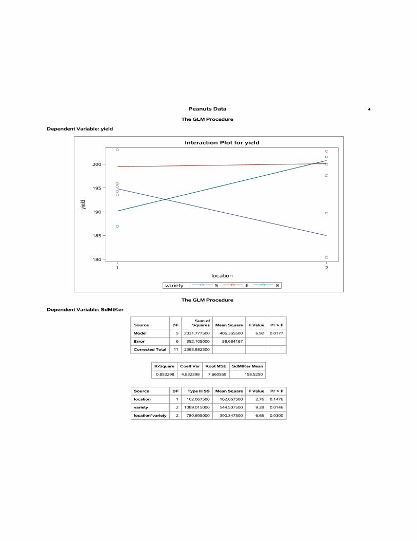
Peanuts Data 4
The GLM Procedure
Dependent Variable: yield
1 2
location
180
185
190
195
200
yield
865variety
Interaction Plot for yield
The GLM Procedure
Dependent Variable: SdMtKer
Source DFSum of
Squares Mean Square F Value Pr > F
Model 5 2031.777500 406.355500 6.92 0.0177
Error 6 352.105000 58.684167
Corrected Total 11 2383.882500
R-Square Coeff Var Root MSE SdMtKer Mean
0.852298 4.832398 7.660559 158.5250
Source DF Type III SS Mean Square F Value Pr > F
location 1 162.067500 162.067500 2.76 0.1476
variety 2 1089.015000 544.507500 9.28 0.0146
location*variety 2 780.695000 390.347500 6.65 0.0300
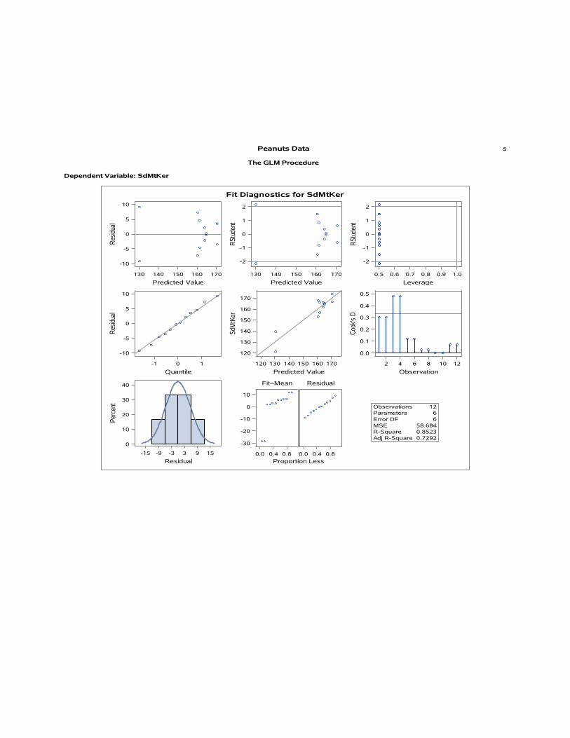
Peanuts Data 5
The GLM Procedure
Dependent Variable: SdMtKer
Fit Diagnostics for SdMtKer
0.7292Adj R-Square0.8523R-Square58.684MSE
6Error DF6Parameters
12Observations
Proportion Less0.0 0.4 0.8
Residual
0.0 0.4 0.8
Fit–Mean
-30
-20
-10
0
10
-15 -9 -3 3 9 15
Residual
0
10
20
30
40
Perc
ent
2 4 6 8 10 12
Observation
0.0
0.1
0.2
0.3
0.4
0.5
Cook
's D
120 130 140 150 160 170
Predicted Value
120
130
140
150
160
170
SdM
tKer
-1 0 1
Quantile
-10
-5
0
5
10
Resid
ual
0.5 0.6 0.7 0.8 0.9 1.0
Leverage
-2
-1
0
1
2
RStu
dent
130 140 150 160 170
Predicted Value
-2
-1
0
1
2
RStu
dent
130 140 150 160 170
Predicted Value
-10
-5
0
5
10
Resid
ual

Peanuts Data 6
The GLM Procedure
Dependent Variable: SdMtKer
1 2
location
120
130
140
150
160
170
SdM
tKer
865variety
Interaction Plot for SdMtKer
The GLM Procedure
Dependent Variable: SeedSize
Source DFSum of
Squares Mean Square F Value Pr > F
Model 5 442.5741667 88.5148333 5.60 0.0292
Error 6 94.8350000 15.8058333
Corrected Total 11 537.4091667
R-Square Coeff Var Root MSE SeedSize Mean
0.823533 7.188166 3.975655 55.30833
Source DF Type III SS Mean Square F Value Pr > F
location 1 72.5208333 72.5208333 4.59 0.0759
variety 2 284.1016667 142.0508333 8.99 0.0157
location*variety 2 85.9516667 42.9758333 2.72 0.1443

Peanuts Data 7
The GLM Procedure
Dependent Variable: SeedSize
Fit Diagnostics for SeedSize
0.6765Adj R-Square0.8235R-Square15.806MSE
6Error DF6Parameters
12Observations
Proportion Less0.0 0.4 0.8
Residual
0.0 0.4 0.8
Fit–Mean
-5
0
5
10
-7.5 -1.5 4.5
Residual
0
10
20
30
40
Perc
ent
2 4 6 8 10 12
Observation
0.0
0.2
0.4
0.6
Cook
's D
45 50 55 60 65
Predicted Value
45
50
55
60
65
Seed
Size
-1 0 1
Quantile
-6
-4
-2
0
2
4
6
Resid
ual
0.5 0.6 0.7 0.8 0.9 1.0
Leverage
-2
0
2
RStu
dent
50 55 60 65
Predicted Value
-2
0
2
RStu
dent
50 55 60 65
Predicted Value
-6
-4
-2
0
2
4
6
Resid
ual

Peanuts Data 8
The GLM Procedure
Dependent Variable: SeedSize
1 2
location
45
50
55
60
65
Seed
Size
865variety
Interaction Plot for SeedSize
The GLM ProcedureMultivariate Analysis of Variance
E = Error SSCP Matrix
yield SdMtKer SeedSize
yield 104.205 49.365 76.48
SdMtKer 49.365 352.105 121.995
SeedSize 76.48 121.995 94.835
Partial Correlation Coefficients from the Error SSCP Matrix / Prob > |r|
DF = 6 yield SdMtKer SeedSize
yield 1.000000 0.2577140.5769
0.7693420.0432
SdMtKer 0.2577140.5769
1.000000 0.6676080.1013
SeedSize 0.7693420.0432
0.6676080.1013
1.000000

Peanuts Data 9
The GLM ProcedureMultivariate Analysis of Variance
H = Type III SSCP Matrix for location
yield SdMtKer SeedSize
yield 0.7008333333 -10.6575 7.1291666667
SdMtKer -10.6575 162.0675 -108.4125
SeedSize 7.1291666667 -108.4125 72.520833333
Characteristic Roots and Vectors of: E Inverse * H, whereH = Type III SSCP Matrix for location
E = Error SSCP Matrix
Characteristic Vector V'EV=1
CharacteristicRoot Percent yield SdMtKer SeedSize
8.38824348 100.00 -0.13688388 -0.07628041 0.23952166
0.00000000 0.00 0.10187838 0.00216080 -0.00678495
0.00000000 0.00 -0.06307410 0.03725453 0.06189287
MANOVATest Criteria and Exact F Statistics for the Hypothesis of No Overall location EffectH = Type III SSCP Matrix for location
E = Error SSCP Matrix
S=1 M=0.5 N=1
Statistic Value F Value Num DF Den DF Pr > F
Wilks' Lambda 0.10651620 11.18 3 4 0.0205
Pillai's Trace 0.89348380 11.18 3 4 0.0205
Hotelling-Lawley Trace 8.38824348 11.18 3 4 0.0205
Roy's Greatest Root 8.38824348 11.18 3 4 0.0205
H = Type III SSCP Matrix for variety
yield SdMtKer SeedSize
yield 196.115 365.1825 42.6275
SdMtKer 365.1825 1089.015 414.655
SeedSize 42.6275 414.655 284.10166667

Peanuts Data 10
The GLM ProcedureMultivariate Analysis of Variance
Characteristic Roots and Vectors of: E Inverse * H, whereH = Type III SSCP Matrix for variety
E = Error SSCP Matrix
Characteristic Vector V'EV=1
CharacteristicRoot Percent yield SdMtKer SeedSize
18.1876113 85.09 -0.16986539 -0.06425268 0.23943636
3.1880638 14.91 0.00137509 0.03769309 0.03800092
0.0000000 0.00 0.06510456 -0.04076880 0.04973481
MANOVATest Criteria and F Approximations for the Hypothesis of No Overall variety EffectH = Type III SSCP Matrix for variety
E = Error SSCP Matrix
S=2 M=0 N=1
Statistic Value F Value Num DF Den DF Pr > F
Wilks' Lambda 0.01244417 10.62 6 8 0.0019
Pillai's Trace 1.70910921 9.79 6 10 0.0011
Hotelling-Lawley Trace 21.37567504 14.25 6 4 0.0113
Roy's Greatest Root 18.18761127 30.31 3 5 0.0012
NOTE: F Statistic for Roy's Greatest Root is an upper bound.
NOTE: F Statistic for Wilks' Lambda is exact.
H = Type III SSCP Matrix for location*variety
yield SdMtKer SeedSize
yield 205.10166667 363.6675 107.78583333
SdMtKer 363.6675 780.695 254.22
SeedSize 107.78583333 254.22 85.951666667
Characteristic Roots and Vectors of: E Inverse * H, whereH = Type III SSCP Matrix for location*variety
E = Error SSCP Matrix
Characteristic Vector V'EV=1
CharacteristicRoot Percent yield SdMtKer SeedSize
6.82409388 90.45 0.15723347 0.06948572 -0.18762316
0.72019649 9.55 -0.08644203 0.01400396 0.12612011
0.00000000 0.00 0.03000259 -0.04676424 0.10069089

Peanuts Data 11
The GLM ProcedureMultivariate Analysis of Variance
MANOVATest Criteria and F Approximations for the Hypothesis of No Overall location*variety EffectH = Type III SSCP Matrix for location*variety
E = Error SSCP Matrix
S=2 M=0 N=1
Statistic Value F Value Num DF Den DF Pr > F
Wilks' Lambda 0.07429984 3.56 6 8 0.0508
Pillai's Trace 1.29086073 3.03 6 10 0.0587
Hotelling-Lawley Trace 7.54429038 5.03 6 4 0.0699
Roy's Greatest Root 6.82409388 11.37 3 5 0.0113
NOTE: F Statistic for Roy's Greatest Root is an upper bound.
NOTE: F Statistic for Wilks' Lambda is exact.
The GLM ProcedureLeast Squares Means
Adjustment for Multiple Comparisons: Bonferroni
variety yield LSMEANLSMEANNumber
5 189.925000 1
6 199.800000 2
8 195.500000 3
Least Squares Means for effect varietyPr > |t| for H0: LSMean(i)=LSMean(j)
Dependent Variable: yield
i/j 1 2 3
1 0.0462 0.3221
2 0.0462 0.5844
3 0.3221 0.5844
variety yield LSMEAN 95% Confidence Limits
5 189.925000 184.826329 195.023671
6 199.800000 194.701329 204.898671
8 195.500000 190.401329 200.598671
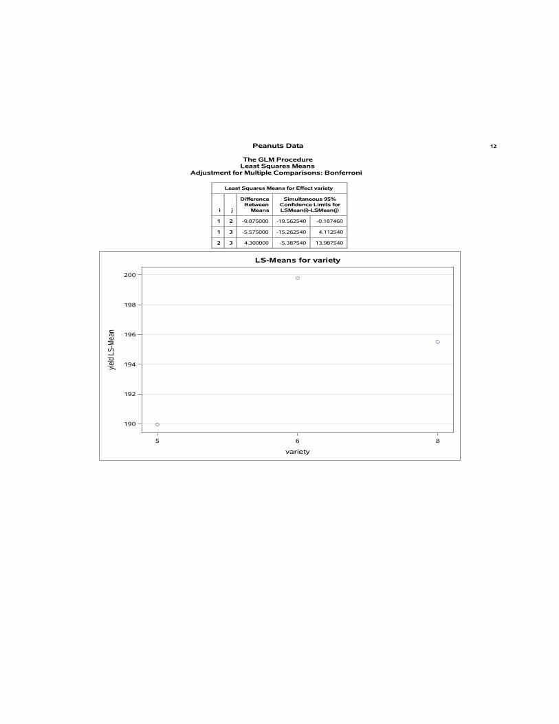
Peanuts Data 12
The GLM ProcedureLeast Squares Means
Adjustment for Multiple Comparisons: Bonferroni
Least Squares Means for Effect variety
i j
DifferenceBetween
Means
Simultaneous 95%Confidence Limits forLSMean(i)-LSMean(j)
1 2 -9.875000 -19.562540 -0.187460
1 3 -5.575000 -15.262540 4.112540
2 3 4.300000 -5.387540 13.987540
190
192
194
196
198
200
yield
LS-M
ean
5 6 8
variety
LS-Means for variety
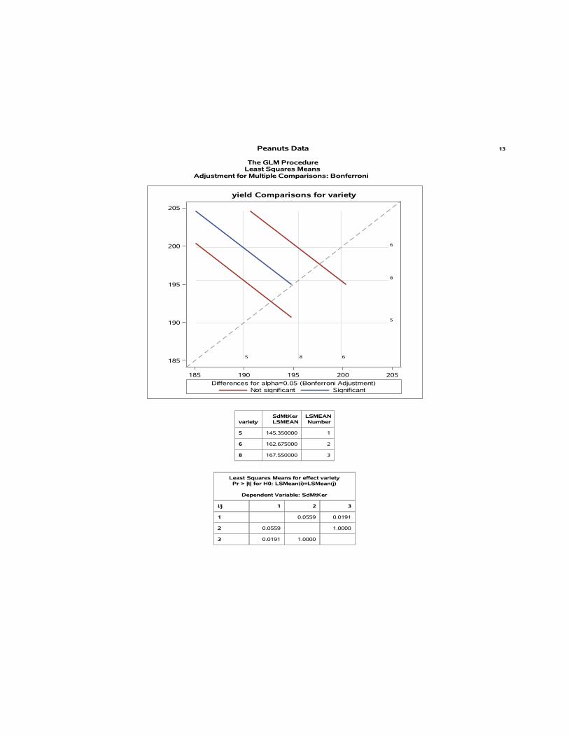
Peanuts Data 13
The GLM ProcedureLeast Squares Means
Adjustment for Multiple Comparisons: Bonferroni
yield Comparisons for variety
SignificantNot significantDifferences for alpha=0.05 (Bonferroni Adjustment)
5 68
5
6
8
185 190 195 200 205
185
190
195
200
205
varietySdMtKerLSMEAN
LSMEANNumber
5 145.350000 1
6 162.675000 2
8 167.550000 3
Least Squares Means for effect varietyPr > |t| for H0: LSMean(i)=LSMean(j)
Dependent Variable: SdMtKer
i/j 1 2 3
1 0.0559 0.0191
2 0.0559 1.0000
3 0.0191 1.0000

Peanuts Data 14
The GLM ProcedureLeast Squares Means
varietySdMtKerLSMEAN 95% Confidence Limits
5 145.350000 135.977644 154.722356
6 162.675000 153.302644 172.047356
8 167.550000 158.177644 176.922356
Least Squares Means for Effect variety
i j
DifferenceBetween
Means
Simultaneous 95%Confidence Limits forLSMean(i)-LSMean(j)
1 2 -17.325000 -35.132597 0.482597
1 3 -22.200000 -40.007597 -4.392403
2 3 -4.875000 -22.682597 12.932597
145
150
155
160
165
SdM
tKer
LS-
Mea
n
5 6 8
variety
LS-Means for variety
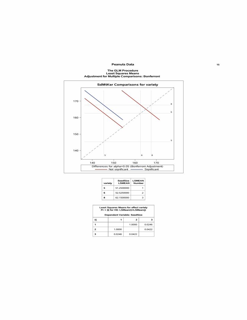
Peanuts Data 15
The GLM ProcedureLeast Squares Means
Adjustment for Multiple Comparisons: Bonferroni
SdMtKer Comparisons for variety
SignificantNot significantDifferences for alpha=0.05 (Bonferroni Adjustment)
5 6 8
5
6
8
140 150 160 170
140
150
160
170
varietySeedSizeLSMEAN
LSMEANNumber
5 51.2500000 1
6 52.5250000 2
8 62.1500000 3
Least Squares Means for effect varietyPr > |t| for H0: LSMean(i)=LSMean(j)
Dependent Variable: SeedSize
i/j 1 2 3
1 1.0000 0.0246
2 1.0000 0.0422
3 0.0246 0.0422

Peanuts Data 16
The GLM ProcedureLeast Squares Means
varietySeedSizeLSMEAN
95%Confidence Limits
5 51.250000 46.385961 56.114039
6 52.525000 47.660961 57.389039
8 62.150000 57.285961 67.014039
Least Squares Means for Effect variety
i j
DifferenceBetween
Means
Simultaneous 95%Confidence Limits forLSMean(i)-LSMean(j)
1 2 -1.275000 -10.516736 7.966736
1 3 -10.900000 -20.141736 -1.658264
2 3 -9.625000 -18.866736 -0.383264
52.5
55.0
57.5
60.0
62.5
Seed
Size
LS-
Mea
n
5 6 8
variety
LS-Means for variety

Peanuts Data 17
The GLM ProcedureLeast Squares Means
Adjustment for Multiple Comparisons: Bonferroni
SeedSize Comparisons for variety
SignificantNot significantDifferences for alpha=0.05 (Bonferroni Adjustment)
5 6 8
5
6
8
50 55 60 65
50
55
60
65
Obs location variety yield SdMtKer SeedSize r1 r2 r3
1 1 5 195.3 153.1 51.4 0.50 -7.30 -1.15
2 1 5 194.3 167.7 53.7 -0.50 7.30 1.15
3 2 5 189.7 139.5 55.5 4.65 9.20 5.55
4 2 5 180.4 121.1 44.4 -4.65 -9.20 -5.55
5 1 6 203.0 156.8 49.8 3.55 -4.60 2.00
6 1 6 195.9 166.0 45.8 -3.55 4.60 -2.00
7 2 6 202.7 166.1 60.4 2.55 2.15 3.15
8 2 6 197.6 161.8 54.1 -2.55 -2.15 -3.15
9 1 8 193.5 164.5 57.8 3.25 -0.30 -0.40
10 1 8 187.0 165.1 58.6 -3.25 0.30 0.40
11 2 8 201.5 166.8 65.0 0.75 -3.50 -1.10
12 2 8 200.0 173.8 67.2 -0.75 3.50 1.10

MULTNORM macro: Univariate and Multivariate Normality Tests 18
The MODEL Procedure
Normality Test
Equation Test Statistic Value Prob
r1 Shapiro-Wilk W 0.95 0.6552
r2 Shapiro-Wilk W 0.98 0.9949
r3 Shapiro-Wilk W 0.99 1.0000
System Mardia Skewness 0.00 1.0000
Mardia Kurtosis -1.14 0.2527
Henze-Zirkler T 0.37 0.8770
0 2 4 6 8
Chi-square quantile
1
2
3
4
5
Squa
red
Dis
tanc
e
MULTNORM macro: Chi-square Q-Q plot

Discriminant Analysis Results 19Discriminant Analysis Results 19
The DISCRIM Procedure
Total Sample Size 12 DF Total 11
Variables 3 DF Within Classes 10
Classes 2 DF Between Classes 1
Number of Observations Read 12
Number of Observations Used 12
Class Level Information
locationVariableName Frequency Weight Proportion
PriorProbability
1 _1 6 6.0000 0.500000 0.500000
2 _2 6 6.0000 0.500000 0.500000
Within Covariance Matrix Information
locationCovariance
Matrix Rank
Natural Log of theDeterminant of theCovariance Matrix
1 3 9.06175
2 3 10.04024
Pooled 3 11.39958
The DISCRIM ProcedureTest of Homogeneity of Within Covariance Matrices
Chi-Square DF Pr > ChiSq
12.477965 6 0.0521
Since the Chi-Square value is significant at the 0.1 level, the within covariance matrices will be used in the discriminantfunction.Reference: Morrison, D.F. (1976) Multivariate Statistical Methods p252.
The DISCRIM Procedure
Generalized Squared Distanceto location
Fromlocation 1 2
1 9.06175 17.74659
2 12.67195 10.04024

Discriminant Analysis Results 20
The DISCRIM ProcedureClassification Summary for Calibration Data: WORK.PEANUTS
Resubstitution Summary using Quadratic Discriminant Function
Number of Observations andPercent Classified into location
Fromlocation 1 2 Total
1 6100.00
00.00
6100.00
2 116.67
583.33
6100.00
Total 758.33
541.67
12100.00
Priors 0.5 0.5
Error Count Estimates forlocation
1 2 Total
Rate 0.0000 0.1667 0.0833
Priors 0.5000 0.5000
The DISCRIM ProcedureClassification Summary for Calibration Data: WORK.PEANUTS
Cross-validation Summary using Quadratic Discriminant Function
Number of Observations andPercent Classified into location
Fromlocation 1 2 Total
1 466.67
233.33
6100.00
2 116.67
583.33
6100.00
Total 541.67
758.33
12100.00
Priors 0.5 0.5
Error Count Estimates forlocation
1 2 Total
Rate 0.3333 0.1667 0.2500
Priors 0.5000 0.5000

Applied Statistics Comprehensive Exam
January 2016
Ph.D Methods Exam
This comprehensive exam consists of 10 questions pertaining to methodological statisticaltopics.
1 This Ph.D level exam will run from 8:30 AM to 3:30 PM.
2 Please label each page with your identification number.
DO NOT USE YOUR NAME OR BEAR NUMBER.
3 Please write only on one side of each page.
4 Please leave one inch margins on all sides of each page.
5 Please number all pages consecutively.
6 Please label the day number (Day 1 or Day 2) on each page.
7 Please begin each question on a new page, and number each question.
8 Please do not staple pages together.
9 No wireless devices, formula sheets, or other outside materials are permitted.
10 Statistical tables and paper will be provided.
11 Relax and good luck!
I have read and understand the rules of this exam.
Signature: Date:

Applied Statistics and Research Methods - January 2016 - Methods Comprehensive 2
1.) Over the past 5 years, an insurance company has had a mix of 40% whole life policies,20% universal life policies, 25% annual renewable-term (ART) policies, and 15% other typesof policies. A change in this mix over the long haul could require a change in the commissionstructure, reserves, and possibly investments. A sample of 1,000 policies issued over the lastfew months gave the results shown here.
Category nWhole life 320
Universal life 280ART 240Other 160
Use these data to assess whether there has been a shift from the historical percentages.Use the 5% significant level. Clearly identify the hypothesis you are testing, report the teststatistic and state your conclusion.
2.) A small travel agency is interested to better understand the effect of age of customer(x) on the amount of money spent in a tour (y), in the last twelve months. Agency hasrecognized two important customer segments. The first segment, which we will denote byA, consists of those customers who have purchased an adventure tour in the last twelvemonths. The second segment, which we will denote by C, consists of those customers whohave purchased a cultural tour in the last twelve months. Note that the two segments arecompletely separate in the sense that there are no customers who are in both segments.Assume the relation between y and x is linear.
i. Write down a single multiple linear model with possibly differing intercepts and slopesfor two different segments of the customers. Interpret each parameter in the model.
ii. Write down the hypothesis that the two lines are coincident in terms of the regressioncoefficients.

Applied Statistics and Research Methods - January 2016 - Methods Comprehensive 3
3.) The effect of five different ingredients A,B,C,D,E on the reaction time of a chemicalprocess is being studied. Each batch of new material is only large enough to permit five runsto be made. Furthermore, each run requires approximatley 1.5 hours, so only five runs canbe made in one day. The experimenter wants to control the two sources of variation andchoses an appropriate design for this.
The data are given in the table below. Answer the following questions.
Table 1: Data for the reaction time of a chemical processBatch Day
1 2 3 4 51 A=8 B=7 C=1 D=7 E=32 B=11 C=2 D=7 E=3 A=83 C=4 D=9 E=10 A=1 B=54 D=6 E=8 A=6 B=6 C=105 E=4 A=2 B=3 C=8 D=8
i. What is the name of this design?
ii. There are two nuisance factors to be “averaged out” in the design. What are those?
iii. Calculate the total corrected sum of squares for this experiment as well as all otherrequired sum of squares.
iv. State the hypothesis, and construct the analysis of variance table including the calcu-lated F -statistic. Comment on the results.
4.) Consider a Two-Factor ANOVA model (with interaction),
Yijk = µ+ αi + βj + (αβ)ij + εijk,
where i = 1, 2, j = 1, 2, 3, and k = 1, 2.
i. Write this model in vector form, showing all components explicitly. Determine therank of your design matrix, X.
ii. Provide an expression for the Least Squares Estimators (LSE) for the parameters ofyour model.
iii. Explain the meaning of the term “estimable.” Why are we concerned with estimability?
iv. Determine whether each of the following functions is estimable:
µ+ α1, β2 − β1, µ+ α1 + β2 + (αβ)12
v. For each of the estimable functions from part iv, provide an expression for the BestLinear Unbiased Estimator, and explain in what sense these are “best”.

Applied Statistics and Research Methods - January 2016 - Methods Comprehensive 4
5.) Amitriptyline is prescribed by some physicians as an antidepressant. However, thereare also conjectured side effects that seem to be related to the use of the drug: irregularheartbeat, abnormal blood pressures, and irregular waves on the electrocardiogram, amongother things. Data gathered on 17 patients who were admitted to the hospital after anamitriptyline overdose are given in the Output 1.1 on Page 7.
The two response (dependent) variables are
Y1 = Total TACD plasma level (TOT)Y2 = Amount of amitriptyline present in TCAD plasma level (AMI)
The five predictor (independent) variables are
X1 = Gender: 1 if female, 0 if male (GEN)X2 = Amount of antidepressants taken at time of overdose (AMT)X3 = PR wave measurement (PR)X4 = Diastolic blood pressure (DIAP)X5 = QRS wave measurement (QRS)
i. Perform a regression analysis using only the first response (Y1). Use Output 1.2 onPage 8 to write the regression model that predicts TOT (Y1) from AMT, PR, DIAP,and QRS. Comment on the overall significance of the model.
ii. Use the fitted model (i.e., the estimated model) above to predict total TCAD plasmalevel (TOT) for a patient whose AMT=750, PR=200, DIAP=80, and QRS=90.
iii. For the model fitted in a), suppose, we are interested in testing for the significance ofAMT in predicting TOT. Write the appropriate null and alternative hypothesis thatyou would be testing for this. Comment on the significance of AMT.
iv. Construct a 95% confidence interval for the parameter associated with AMT. Commenton the interval. Is the CI consistent with the test result in part iii?
v. Suppose you would like to test for significance of AMT and DIAP together. For thiswe would perform a partial F-test by fitting two models–one with all the predictors,and the other without AMT and DIAP. See the Output 1.3 on Page 9.
Write appropriate null and alternative hypotheses and carry out the test. Calculatethe value of the appropriate test statistic. Comment on your findings.
vi. List the assumptions concerning the model fitted in part i. Analyze the residuals. Arethere any sign of violation of any of the regression assumptions?

Applied Statistics and Research Methods - January 2016 - Methods Comprehensive 5
6.) Suppose a design of Resolution III is desired for N − 1 = 7 factors in N = 8 runs. Eachfactor is considered to have two levels– low and high. The eight runs would be a 1/16thfraction of the 27 = 128 runs. This design is a 27−4
III fractional factorial. Suppose the designgenerators are ABD, ACE, BCF , and ABCG.
Answer the following questions.
i. Construct the standard order table for the above design.
ii. Show/derive the complete defining relation for the above design.
iii. Show the complete alias structure for the above design.
iv. When do you think such a design would be applicable. Give a real life example withdetails of factors and their levels.
7.) Given the data, use the Wilcoxon Signed Ranks Test to test:
H0 : µ = 107 vs H1 : µ 6= 107.
99, 100, 90, 94, 135, 108, 107, 111, 119, 104, 127, 109, 117, 105, 125
8.) A researcher wishes to estimate the average income of employees in a large firm. Recordshave the employees listed by seniority, and, generally speaking, salary increases with seniority.Discuss the relative merits of simple random sampling and stratified random sampling in thiscase.

Applied Statistics and Research Methods - January 2016 - Methods Comprehensive 6
9.) The carbonation level of a soft drink beverage is affected by the temperature of theproduct and the filler operating pressure. Twelve observations were obtained and analyzedusing SAS software. Use the SAS output on Page 10 to answer the following questions.
i. Fit a second-order polynomial.
ii. Test for significance of regression.
iii. What is the lack of fit test for? Why can we do this test for this data set? Test forlack of fit and draw conclusions.
iv. Does the interaction term contribute significantly to the model?
v. Do the second-order terms contribute significantly to the model?
vi. Is there any sign of multicollinearity? If yes, how would you deal with it?
10.) A financial analyst is interested in factors that impact fraudulent activity on credit cards.Using historical data, she has collected monthly counts of fraudulent activities identified onvarious credit cards supported by regional stores. She has also recorded whether each cardis available for international use, whether each card was made available to individuals underthe age of 18, whether each card was awarded with a promotional gift, and a continuousmeasure of each card’s monthly usage volume. The analyst would like to determine whetherany of the recorded factors has an effect on the volume of monthly fraudulent activities.
i. Propose some descriptive statistics that could be used to help answer the analyst’squestions.
ii. Using the SAS output on Pages 11-13, describe the response of interest, monthly fraud-ulent activities.
iii. Propose an appropriate model that could be used to determine whether any of theassociated factors affect monthly fraudulent activity.
iv. Using the SAS output on Pages 11-13, perform an analysis of the data. Be sure topresent conclusions using the language of the original question.
v. Suppose the experiment is expanded to include all US credit cards. When the analystcollects a similar but larger data set, she notices that approximately 40% of the obser-vations are zeros. How would you change your analysis approach to account for thisphenomenon?

Applied Statistics and Research Methods - January 2016 - Methods Comprehensive 7
SAS Output for Question 5
Output 1.1: Drug Overdose Data Set
1
Obs tot ami gen amt pr diap qrs
1 3389 3149 1 7500 220 0 140
2 1101 653 1 1975 200 0 100
3 1131 810 0 3600 205 60 111
4 596 448 1 675 160 60 120
5 896 844 1 750 185 70 83
6 1767 1450 1 2500 180 60 80
7 807 493 1 350 154 80 98
8 1111 941 0 1500 200 70 93
9 645 547 1 375 137 60 105
10 628 392 1 1050 167 60 74
11 1360 1283 1 3000 180 60 80
12 652 458 1 450 160 64 60
13 860 722 1 1750 135 90 79
14 500 384 0 2000 160 60 80
15 781 501 0 4500 180 0 100
16 1070 405 0 1500 170 90 120
17 1754 1520 1 3000 180 0 129
The REG Procedure Model: MODEL1
Dependent Variable: tot
Analysis of Variance
Source DF Sum of
Squares Mean
Square F Value Pr > F
Model 4 5461108 1365277 7.30 0.0032
Error 12 2244832 187069
Corrected Total 16 7705940

Applied Statistics and Research Methods - January 2016 - Methods Comprehensive 8
SAS Output for Question 5
Output 1.2 Regression of AMT PR DIAP QRS on TOT
2
Parameter Estimates
Variable DF Parameter
Estimate Standard
Error t Value Pr > |t| Variance Inflation
95% Confidence Limits
Intercept 1 -1308.68851 1245.59727 -1.05 0.3141 0 -4022.61182 1405.23481
amt 1 0.24839 0.09271 2.68 0.0201 2.45782 0.04641 0.45038
pr 1 6.41246 6.38695 1.00 0.3352 1.88054 -7.50352 20.32844
diap 1 3.06008 4.71297 0.65 0.5284 1.86750 -7.20860 13.32877
qrs 1 6.33545 5.90093 1.07 0.3041 1.39799 -6.52157 19.19247
Fit Diagnostics for tot
0.6116Adj R-Square0.7087R-Square187069MSE
12Error DF5Parameters
17Observations
Proportion Less0.0 0.4 0.8
Residual
0.0 0.4 0.8
Fit–Mean
-500
0
500
1000
1500
-1200 -300 600Residual
0
10
20
30
40
50
Perce
nt
0 5 10 15Observation
0.00
0.25
0.50
0.75
1.00
1.25
Cook
's D
1000 2000 3000Predicted Value
1000
2000
3000
tot
-2 -1 0 1 2Quantile
-500
0
500
Resid
ual
0.2 0.3 0.4 0.5 0.6Leverage
-2
0
2
RStud
ent
500 1500 2500Predicted Value
-2
0
2
RStud
ent
500 1500 2500Predicted Value
-500
0
500
Resid
ual

Applied Statistics and Research Methods - January 2016 - Methods Comprehensive 9
SAS Output for Question 5
Output 1.3 Partial Significance of AMT and DIAP
3
The REG Procedure Model: FullModel
Dependent Variable: tot
Analysis of Variance
Source DF Sum of
Squares Mean
Square F Value Pr > F
Model 4 5461108 1365277 7.30 0.0032
Error 12 2244832 187069
Corrected Total 16 7705940
Parameter Estimates
Variable DF Parameter
Estimate Standard
Error t Value Pr > |t|
Intercept 1 -1308.68851 1245.59727 -1.05 0.3141
amt 1 0.24839 0.09271 2.68 0.0201
pr 1 6.41246 6.38695 1.00 0.3352
diap 1 3.06008 4.71297 0.65 0.5284
qrs 1 6.33545 5.90093 1.07 0.3041
The REG Procedure
Model: Submodel Dependent Variable: tot
Analysis of Variance
Source DF Sum of
Squares Mean
Square F Value Pr > F
Model 2 4081088 2040544 7.88 0.0051
Error 14 3624853 258918
Corrected Total 16 7705940
Parameter Estimates
Variable DF Parameter
Estimate Standard
Error t Value Pr > |t|
Intercept 1 -2675.83752 989.89628 -2.70 0.0172
pr 1 15.57400 5.94574 2.62 0.0202
qrs 1 11.03858 6.37119 1.73 0.1051
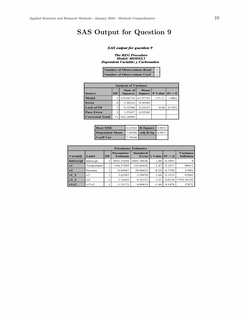
Applied Statistics and Research Methods - January 2016 - Methods Comprehensive 10
SAS Output for Question 9
SAS output for question 9
The REG ProcedureModel: MODEL1
Dependent Variable: y Carbonation
SAS output for question 9
The REG ProcedureModel: MODEL1
Dependent Variable: y Carbonation
Number of Observations Read 12
Number of Observations Used 12
Analysis of Variance
Source DFSum of
SquaresMean
Square F Value Pr > F
Model 5 339.88774 67.97755 177.17 <.0001
Error 6 2.30216 0.38369
Lack of Fit 3 0.72590 0.24197 0.46 0.7297
Pure Error 3 1.57627 0.52542
Corrected Total 11 342.18990
Root MSE 0.61943 R-Square 0.9933
Dependent Mean 7.94500 Adj R-Sq 0.9877
Coeff Var 7.79648
Parameter Estimates
Variable Label DFParameter
EstimateStandard
Error t Value Pr > |t|VarianceInflation
Intercept Intercept 1 3025.31858 2045.74638 1.48 0.1897 0
x1 Temperature 1 -194.27289 132.06428 -1.47 0.1917 90911
x2 Pressure 1 -6.05067 20.60625 -0.29 0.7789 15401
x1_2 x1² 1 3.62587 2.20978 1.64 0.1519 97845
x2_2 x2² 1 1.15425 0.32373 3.57 0.0118 7759.76159
x1x2 x1*x2 1 -1.33171 0.89619 -1.49 0.1878 37872

Applied Statistics and Research Methods - January 2016 - Methods Comprehensive 11
SAS Output for Question 10
Moments
N 40 Sum Weights 40
Mean 8.9 Sum Observations 356
Std Deviation 14.9611463 Variance 223.835897
Skewness 2.18258178 Kurtosis 4.05213894
Uncorrected SS 11898 Corrected SS 8729.6
Coeff Variation 168.102767 Std Error Mean 2.36556493

Applied Statistics and Research Methods - January 2016 - Methods Comprehensive 12
SAS Output for Question 10
Model Information
Data Set WORK.CREDITDATA
Distribution Negative Binomial
Link Function Log
Dependent Variable FraudulentActivities
Number of Observations Read 40
Number of Observations Used 34
Missing Values 6
Criteria For Assessing Goodness Of Fit
Criterion DF Value Value/DF
Deviance 27 57.1062 2.1150
Scaled Deviance 27 57.1062 2.1150
Pearson Chi-Square 27 53.0935 1.9664
Scaled Pearson X2 27 53.0935 1.9664
Log Likelihood 758.8075
Full Log Likelihood -77.4864
AIC (smaller is better) 168.9727
AICC (smaller is better) 173.2804
BIC (smaller is better) 179.6573
Algorithm converged.

Applied Statistics and Research Methods - January 2016 - Methods Comprehensive 13
SAS Output for Question 10
Analysis Of Maximum Likelihood Parameter Estimates
Parameter DF Estimate Standard
Error
Wald 95% Confidence
Limits Wald Chi-
Square Pr > ChiSq
Intercept 1 -2.7512 1.0850 -4.8778 -0.6246 6.43 0.0112
International 1 -2.7066 1.4921 -5.6311 0.2178 3.29 0.0697
Under18 1 -1.5216 1.1519 -3.7792 0.7360 1.75 0.1865
GiftPromotion 1 0.1837 0.1301 -0.0713 0.4387 1.99 0.1580
UsageVolume 1 0.6157 0.1327 0.3556 0.8757 21.53 <.0001
Under18*UsageVolume 1 0.2073 0.1400 -0.0671 0.4817 2.19 0.1387
Internati*UsageVolum 1 0.2341 0.1653 -0.0899 0.5582 2.01 0.1568
Dispersion 0 0.0000 0.0000 . .
Note: The negative binomial dispersion parameter was held fixed.
Lagrange Multiplier Statistics
Parameter Chi-Square Pr > ChiSq
Dispersion 0.8224 0.1822 *
* One-sided p-value

Applied Statistics Comprehensive Exam
January 2017
Ph.D Methods Exam
This comprehensive exam consists of 10 questions pertaining to methodological statisticaltopics.
1 This Ph.D level exam will run from 8:30 AM to 3:30 PM.
2 Please label each page with your identification number.
DO NOT USE YOUR NAME OR BEAR NUMBER.
3 Please write only on one side of each page.
4 Please leave one inch margins on all sides of each page.
5 Please number all pages consecutively.
6 Please label the day number (Day 1 or Day 2) on each page.
7 Please begin each question on a new page, and number each question.
8 Please do not staple pages together.
9 No wireless devices, formula sheets, or other outside materials are permitted.
10 Statistical tables and paper will be provided.
11 Relax and good luck!
I have read and understand the rules of this exam.
Signature: Date:

Applied Statistics and Research Methods - January 2017 - Methods Comprehensive 2
1.) Briefly describe the experimental design you would choose for each of the followingsituations, and explain why.
i. An investigative group at a television station wishes to determine if doctors treat pa-tients on public assistance differently from those with private insurance. They measurethis by how long the doctor spends with the patient. There are four large clinics in thecity, and the station chooses three pediatricians at random from each of the four clin-ics. Ninety-six families on public assistance are located and divided into four groupsof 24 at random. All 96 families have a one-year-old child and a child just enteringschool. Half the families will request a one-year checkup, and the others will requesta preschool checkup. Half the families will be given temporary private insurance forthe study, and the others will use public assistance. The four groupings of familiesare the factorial combinations of checkup type and insurance type. Each group of 24is now divided at random into twelve sets of two, with each set of two assigned toone of the twelve selected doctors. Thus each doctor will see eight patients from theinvestigation. Recap: 96 units (families); the response is how long the doctor spendswith each family.
ii. Food scientists wish to study how urban and rural consumers rate cheddar cheesesfor bitterness. Four 50-pound blocks of cheddar cheese of different types are obtained.Each block of cheese represents one of the segments of the market (for example, a sharpNew York style cheese). The raters are students from a large introductory food scienceclass. Ten students from rural backgrounds and ten students from urban backgroundsare selected at random from the pool of possible raters. Each rater will taste eightbites of cheese presented in random order. The eight bites are two each from thefour different cheeses, but the raters don’t know that. Each rater rates each bite forbitterness.
iii. A small travel agency is interested to better understand the effect of age of customer(x) on the amount of money spent in a tour (y), in the last twelve months. Agencyhas recognized two important customer segments. The first segment, which we willdenote by A, consists of those customers who have purchased an adventure tour in thelast twelve months. The second segment, which we will denote by C, consists of thosecustomers who have purchased a cultural tour in the last twelve months. Note thatthe two segments are completely separate in the sense that there are no customers whoare in both segments.
2.) In an experiment to investigate the effect of color of paper (blue,green, orange) onresponse rates for questionnaires distributed by the “windshield method” in supermarketparking lots, 15 representative supermarket parking lots were chosen in a metropolitan areaand each color was assigned at random to five of the lots. It has been suggested to theinvestigator that size of parking lot might be a useful concomitant variable. For this questionuse the SAS output on Page 6.
i. Test for color effects after adjusting for the size of parking lot; use α = .10.
ii. Make all pairwise comparisons between the color effects after adjusting for the size ofparking lot; use the Bonferroni procedure with a .05 percent family rate. Also use theadjusted MSE for the denominator of your t-tests.

Applied Statistics and Research Methods - January 2017 - Methods Comprehensive 3
3.) Kuehl (2000) reports the results of an experiment conducted at a large seafood companyto investigate the effect of storage temperature and type of seafood upon bacterial growth onoysters and mussels. Three storage temperatures were studied (0◦C, 5◦C, and 10◦C). Threecold storage units were randomly assigned to be operated at each temperature. Within eachstorage unit, oysters and mussels were randomly assigned to be stored on one of the twoshelves. The seafood was stored for 2 weeks at the assigned temperature, and at the end ofthe time the bacterial count was obtained from a sample on each shelf. The resulting data(log bacterial count) is shown below.
Storage Seafood TypeUnit Temp. Oysters Mussels
1 0 3.6882 0.35652 0 1.8275 1.70233 0 5.2327 4.57804 5 7.1950 5.01695 5 9.3224 7.95196 5 7.4195 6.38617 10 9.7842 10.13528 10 6.4703 5.04829 10 9.4442 11.0329
i. What is the experimental unit for temperature?
ii. Why was it necessary to include nine storage units instead of three?
iii. What is the experimental unit for seafood type?
iv. What design was used to conduct the experiment? Justify your answer. In particular,write the factors, their levels, and the outcome variable.
v. Write the statistical model for the data and identify the model components.
vi. List the assumptions that need to be checked for the model that you considered above.
4.) Consider the model,
y1 = θ1 + θ2 + ε1,
y2 = 2θ1 + ε2,
y3 = θ1 − θ2 + ε3.
where εi, i = 1, 2, 3 are i.i.d. N(0, σ2). Assume yT =[2 1 4
]is observed.
i. Find a 95% confidence intervals for θ1 − θ2.
ii. Find the value of the GLRT test statistic for testing H0 : θ1 = θ2 versus Ha : θ1 6= θ2.
iii. What is your conclusion for the hypothesis in (ii)?

Applied Statistics and Research Methods - January 2017 - Methods Comprehensive 4
5.) The following data are a random sample from a three variates normal distribution.
SubjectNumber y1 y2 y3
1 51 36 502 27 20 263 37 22 414 42 36 325 27 18 336 43 32 437 41 22 368 38 21 319 36 23 2710 26 31 3111 29 20 25
Here are the sample mean vector and sample covariance matrix of the above data:
y =
36.0925.5534.09
, S =
65.09 33.65 47.5933.65 46.07 28.9547.59 28.95 60.69
Using these data, at the level of significance 0.05, perform the following testing of hypothesisand report your conclusion.
H0 : µ =
302025
against Ha : µ 6=
302025
.6.) Explain in your words the purpose of response surface methods in the context of designand analysis of an experiment. In particular attempt to explain the following items:
i. Provide a brief outline of response surface methodology.
ii. What are the key differences and similarities of response surface design with a 2k
factorial experiment? When would you perform a response surface analysis?
iii. Illustrate with diagrams or figures the three types of stationary points that come alongwith a response surface analysis.
7.) Given the data, use the Sign Test to test H0 : µ = 8.41 versus H1 : µ > 8.41.
8.30, 9.50, 9.60, 8.75, 8.40, 9.10, 9.25, 9.80, 10.05, 8.15, 10.00, 9.60, 9.80, 9.20, 9.30
8.) A researcher wishes to estimate the average income of employees in a large firm. Recordshave the employees listed by seniority, and, generally speaking, salary increases with seniority.Discuss the relative merits of simple random sampling and stratified random sampling in thiscase.

Applied Statistics and Research Methods - January 2017 - Methods Comprehensive 5
9.) In the SAS output on Pages 7-8 you see analysis of a data set. Based on this output,answer the following questions.
i. Test H0 : β1 = β2 = β3 = β4 = β5 = 0.
ii. Do you see any evidence of multicollinearity? Give your reasons?
iii. What criteria is chosen for model selection? What is the best selected model?
iv. Do you think the best selected model has taken care of the multicollinearity?
10.) Housing finance researchers are interested in predicting current college students’ chancesof living in various levels of housing in five years, using parents’ income (in thousands ofdollars per year), gender (female, male), and race (African-American, Caucasian, Hispanic/ Latino) as predictors. The researchers conducted a retrospective study in which 20 formercollege students (approximately five years removed from college) were randomly selected fromeach of the six combinations of gender and race (giving 120 total subjects). Each subjectwas asked to estimate his/her parents’ annual income and to indicate whether he/she rentsan apartment, rents a condo or townhouse, owns a condo or townhouse (without land), orowns a house (with land).
i. Propose an appropriate Generalized Linear Model (GLM) to predict the chances ofreaching each level of housing. Clearly explain the meaning of each component andeach parameter included in your model.
ii. Compare your proposed model from part i with at least one other possible model usinga different link function.
iii. Assuming all 120 subjects provide different values for “parents’ income,” calculate the“error” degrees of freedom for your model.
iv. Explain the meaning of the “proportional odds assumption.” Does your model includesuch an assumption?
v. Suppose a single parameter for “parents’ income” is estimated to be β ≈ 0.55. Providean interpretation of this parameter estimate.

Applied Statistics and Research Methods - January 2017 - Methods Comprehensive 6
SAS output for Question 2Q2
The GLM Procedure
Dependent Variable: response rate
Q2
The GLM Procedure
Dependent Variable: response rate
Source DFSum of
Squares Mean Square F Value Pr > F
Model 3 122.6838120 40.8946040 341.78 <.0001
Error 11 1.3161880 0.1196535
Corrected Total 14 124.0000000
R-Square Coeff Var Root MSE response rate Mean
0.989386 1.192792 0.345910 29.00000
Source DF Type I SS Mean Square F Value Pr > F
Color 2 7.6000000 3.8000000 31.76 <.0001
size 1 115.0838120 115.0838120 961.81 <.0001
Source DF Type III SS Mean Square F Value Pr > F
Color 2 23.3918639 11.6959320 97.75 <.0001
size 1 115.0838120 115.0838120 961.81 <.0001
Q2
The GLM ProcedureLeast Squares Means
Q2
The GLM ProcedureLeast Squares Means
Color
responserate
LSMEAN
Blue 29.1436089
Green 30.4884248
Orange 27.3679662

Applied Statistics and Research Methods - January 2017 - Methods Comprehensive 7
SAS output for Question 9
The SAS System
Model: MODEL1Dependent Variable: y y
The SAS System
Model: MODEL1Dependent Variable: y y
Number of Observations Read 27
Number of Observations Used 27
Analysis of Variance
Source DFSum of
SquaresMean
Square F Value Pr > F
Model 7 5729.27961 818.46852 7.26 0.0003
Error 19 2140.83249 112.67539
Corrected Total 26 7870.11210
Root MSE 10.61487 R-Square 0.7280
Dependent Mean 24.73037 Adj R-Sq 0.6278
Coeff Var 42.92239
Parameter Estimates
Variable Label DFParameter
EstimateStandard
Error t Value Pr > |t| Type I SS Type II SSVarianceInflation
Intercept Intercept 1 53.93702 57.42895 0.94 0.3594 16513 99.38965 0
x1 x1 1 -0.12765 0.28150 -0.45 0.6553 3909.46676 23.17091 3.67457
x2 x2 1 -0.22918 0.23264 -0.99 0.3370 0.06700 109.34435 7.72641
x3 x3 1 0.82485 0.76527 1.08 0.2946 271.28437 130.90367 19.20339
x4 x4 1 -0.43822 0.35855 -1.22 0.2366 49.20818 168.31209 7.46364
x5 x5 1 -0.00194 0.00965 -0.20 0.8431 417.17861 4.53643 4.69700
x6 x6 1 0.01989 0.00809 2.46 0.0237 704.98814 681.08914 7.73152
x7 x7 1 1.99349 1.08970 1.83 0.0831 377.08655 377.08655 1.11945
The SAS System
Model: MODEL1Dependent Variable: y y
Collinearity Diagnostics
Proportion of Variation
Number EigenvalueCondition
Index Intercept x1 x2 x3 x4 x5 x6 x7
1 6.32655 1.00000 0.00003102 0.00144 0.00001004 0.00002864 0.00060092 0.00133 0.00076761 0.00649
2 1.06079 2.44213 0.00000145 0.02325 3.02933E-7 0.00001692 0.00447 0.01945 0.01134 0.00918
3 0.43116 3.83055 0.00003233 0.00084028 0.00000755 0.00001076 0.00042097 0.00878 0.00448 0.88354
4 0.08564 8.59496 0.00027294 0.42757 0.00001098 0.00023206 0.19501 0.00024423 0.00205 0.00078779
5 0.06036 10.23816 0.00271 0.19364 0.00086074 0.00134 0.03862 0.55978 0.02657 0.03168
6 0.03157 14.15552 0.00190 0.16202 0.00085247 0.00251 0.06273 0.39946 0.76762 0.02151
7 0.00367 41.54161 0.16062 0.13203 0.00015639 0.15720 0.25780 0.00495 0.09246 0.04614
8 0.00026063 155.80205 0.83442 0.05921 0.99810 0.83866 0.44035 0.00600 0.09472 0.00067480

Applied Statistics and Research Methods - January 2017 - Methods Comprehensive 8
SAS output for Question 9-cont’dThe SAS System
Model: MODEL2Dependent Variable: y
C(p) Selection Method
The SAS System
Model: MODEL2Dependent Variable: y
C(p) Selection Method
Number of Observations Read 27
Number of Observations Used 27
Number inModel C(p) R-Square Variables in Model
2 -0.0208 0.6996 x6 x7
The SAS System
Model: MODEL2Dependent Variable: y y
The SAS System
Model: MODEL2Dependent Variable: y y
Number of Observations Read 27
Number of Observations Used 27
Analysis of Variance
Source DFSum of
SquaresMean
Square F Value Pr > F
Model 2 5506.27694 2753.13847 27.95 <.0001
Error 24 2363.83516 98.49313
Corrected Total 26 7870.11210
Root MSE 9.92437 R-Square 0.6996
Dependent Mean 24.73037 Adj R-Sq 0.6746
Coeff Var 40.13030
Parameter Estimates
Variable Label DFParameter
EstimateStandard
Error t Value Pr > |t| Type I SS Type II SSVarianceInflation
Intercept Intercept 1 2.52646 3.61005 0.70 0.4908 16513 48.23955 0
x6 x6 1 0.01852 0.00275 6.74 <.0001 5008.93619 4476.98336 1.02039
x7 x7 1 2.18575 0.97270 2.25 0.0341 497.34075 497.34075 1.02039
The SAS System
Model: MODEL2Dependent Variable: y y
Collinearity Diagnostics
Proportion of Variation
Number EigenvalueCondition
Index Intercept x6 x7
1 2.44190 1.00000 0.04111 0.04703 0.05975
2 0.37728 2.54410 0.03123 0.28130 0.81885
3 0.18082 3.67487 0.92766 0.67167 0.12141

Applied Statistics Comprehensive Exam
January 2018
Ph.D Methods Exam
This comprehensive exam consists of 10 questions pertaining to methodological statisticaltopics.
1 This Ph.D level exam will run from 8:30 AM to 3:30 PM.
2 Please label each page with your identification number.
DO NOT USE YOUR NAME OR BEAR NUMBER.
3 Please write only on one side of each page.
4 Please leave one inch margins on all sides of each page.
5 Please number all pages consecutively.
6 Please label the day number (Day 1 or Day 2) on each page.
7 Please begin each question on a new page, and number each question.
8 Please do not staple pages together.
9 No wireless devices, formula sheets, or other outside materials are permitted.
10 Statistical tables and paper will be provided.
11 Relax and good luck!
I have read and understand the rules of this exam.
Signature: Date:
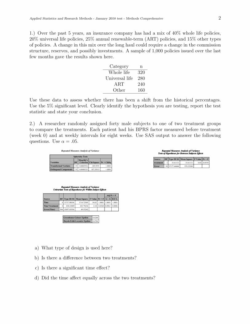
Applied Statistics and Research Methods - January 2018 test - Methods Comprehensive 2
1.) Over the past 5 years, an insurance company has had a mix of 40% whole life policies,20% universal life policies, 25% annual renewable-term (ART) policies, and 15% other typesof policies. A change in this mix over the long haul could require a change in the commissionstructure, reserves, and possibly investments. A sample of 1,000 policies issued over the lastfew months gave the results shown here.
Category nWhole life 320
Universal life 280ART 240Other 160
Use these data to assess whether there has been a shift from the historical percentages.Use the 5% significant level. Clearly identify the hypothesis you are testing, report the teststatistic and state your conclusion.
2.) A researcher randomly assigned forty male subjects to one of two treatment groupsto compare the treatments. Each patient had his BPRS factor measured before treatment(week 0) and at weekly intervals for eight weeks. Use SAS output to answer the followingquestions. Use α = .05. Q5
The GLM ProcedureRepeated Measures Analysis of Variance
Sphericity Tests
Variables DFMauchly's
Criterion Chi-Square Pr > ChiSq
Transformed Variates 35 0.0002916 285.9191 <.0001
Orthogonal Components 35 0.0048335 187.29315 <.0001
Q5
The GLM ProcedureRepeated Measures Analysis of Variance
Tests of Hypotheses for Between Subjects Effects
Q5
The GLM ProcedureRepeated Measures Analysis of Variance
Tests of Hypotheses for Between Subjects Effects
Source DF Type III SS Mean Square F Value Pr > F
treatment 1 33.61111 33.61111 0.03 0.8539
Error 38 37177.44444 978.35380
Q5
The GLM ProcedureRepeated Measures Analysis of Variance
Univariate Tests of Hypotheses for Within Subject Effects
Q5
The GLM ProcedureRepeated Measures Analysis of Variance
Univariate Tests of Hypotheses for Within Subject Effects
Adj Pr > F
Source DF Type III SS Mean Square F Value Pr > F G - G H-F-L
Time 8 13717.80556 1714.72569 34.62 <.0001 <.0001 <.0001
Time*treatment 8 830.33889 103.79236 2.10 0.0360 0.0961 0.0886
Error(Time) 304 15057.85556 49.53242
Greenhouse-Geisser Epsilon 0.4240
Huynh-Feldt-Lecoutre Epsilon 0.4706
a) What type of design is used here?
b) Is there a difference between two treatments?
c) Is there a significant time effect?
d) Did the time affect equally across the two treatments?

Applied Statistics and Research Methods - January 2018 test - Methods Comprehensive 3
3.) A drug company claims that a certain vitamin will increase a sprinter’s speed in the200 yard dash. Eight runners were initially timed (in sec.), given the supplement, and thentimed again on the next day.
Athlete: 1 2 3 4 5 6 7 8
Day one: 21.0 23.0 18.2 20.5 26.2 25.3 21.9 21.6
Day two: 21.9 23.6 17.9 20.4 27.0 25.0 22.2 21.6
Test for a vitamin effect using α = .05. State the null and alternate hypotheses, and reportthe value of the test statistic, and the critical value used to conduct the test. Report yourdecision regarding the null hypothesis and your conclusion in the context of the problem.
4.) Briefly describe the experimental design you would choose for each of the followingsituations, and explain why.
a) Modern zoos try to reproduce natural habitats in their exhibits as much as possible.They therefore use appropriate plants, but these plants can be infested with inappropri-ate insects. Zoos need to take great care with pesticides, because the variety of speciesin a zoo makes it more likely that a sensitive species is present. Cycads (plants that lookvaguely like palms) can be infested with mealybug, and the zoo wishes to test threetreatments: water (a control), horticultural oil (a standard no-mammalian-toxicitypesticide), and fungal spores in water (Beauveria bassiana, a fungus that grows exclu-sively on insects). Five infested cycads are removed to a testing area. Three branchesare randomly chosen on each cycad, and two 3 cm by 3 cm patches are marked oneach branch; the number of mealybugs in these patches is noted. The three brancheson each cycad are randomly assigned to the three treatments. After three days, thepatches are counted again, and the response is the change in the number of mealybugs(before - after).
b) An investigative group at a television station wishes to determine if doctors treat pa-tients on public assistance differently from those with private insurance. They measurethis by how long the doctor spends with the patient. There are four large clinics in thecity, and the station chooses three pediatricians at random from each of the four clin-ics. Ninety-six families on public assistance are located and divided into four groupsof 24 at random. All 96 families have a one-year-old child and a child just enteringschool. Half the families will request a one-year checkup, and the others will requesta preschool checkup. Half the families will be given temporary private insurance forthe study, and the others will use public assistance. The four groupings of familiesare the factorial combinations of checkup type and insurance type. Each group of 24is now divided at random into twelve sets of two, with each set of two assigned toone of the twelve selected doctors. Thus each doctor will see eight patients from theinvestigation. Recap: 96 units (families); the response is how long the doctor spendswith each family.
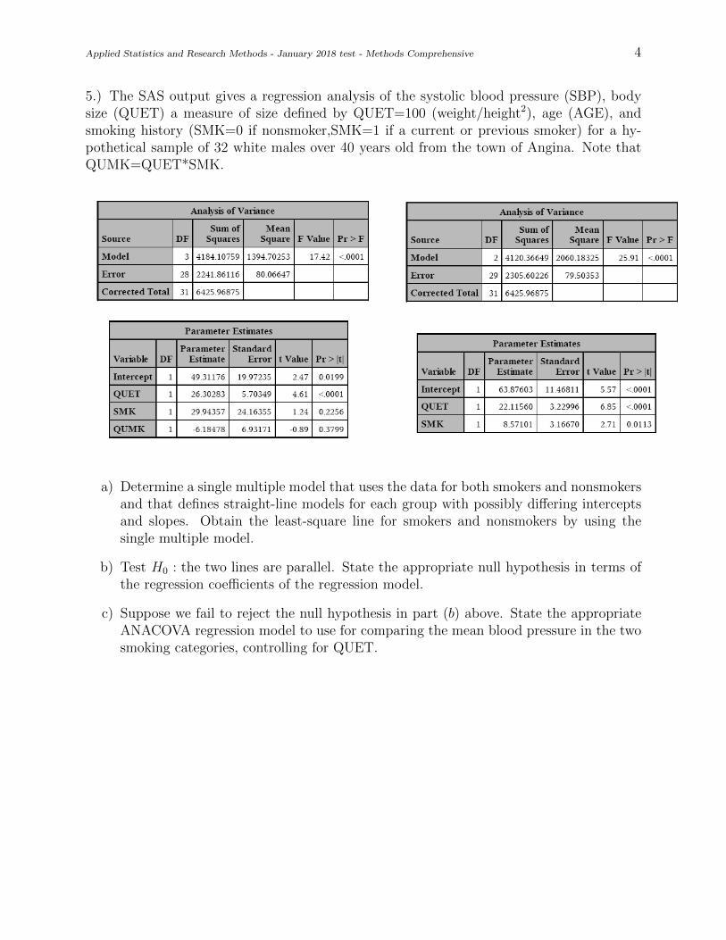
Applied Statistics and Research Methods - January 2018 test - Methods Comprehensive 4
5.) The SAS output gives a regression analysis of the systolic blood pressure (SBP), bodysize (QUET) a measure of size defined by QUET=100 (weight/height2), age (AGE), andsmoking history (SMK=0 if nonsmoker,SMK=1 if a current or previous smoker) for a hy-pothetical sample of 32 white males over 40 years old from the town of Angina. Note thatQUMK=QUET*SMK.
a) Determine a single multiple model that uses the data for both smokers and nonsmokersand that defines straight-line models for each group with possibly differing interceptsand slopes. Obtain the least-square line for smokers and nonsmokers by using thesingle multiple model.
b) Test H0 : the two lines are parallel. State the appropriate null hypothesis in terms ofthe regression coefficients of the regression model.
c) Suppose we fail to reject the null hypothesis in part (b) above. State the appropriateANACOVA regression model to use for comparing the mean blood pressure in the twosmoking categories, controlling for QUET.
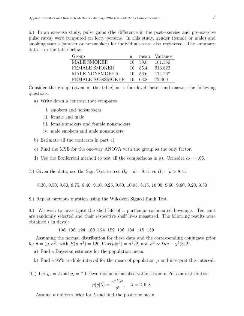
Applied Statistics and Research Methods - January 2018 test - Methods Comprehensive 5
6.) In an exercise study, pulse gains (the difference in the post-exercise and pre-exercisepulse rates) were computed on forty persons. In this study, gender (female or male) andsmoking status (smoker or nonsmoker) for individuals were also registered. The summarydata is in the table below.
Group n mean VarianceMALE SMOKER 10 59.0 101.556FEMALE SMOKER 10 85.4 913.822MALE NONSMOKER 10 56.6 174.267FEMALE NONSMOKER 10 63.8 72.400
Consider the group (given in the table) as a four-level factor and answer the followingquestions.
a) Write down a contrast that compares
i. smokers and nonsmokers
ii. female and male
iii. female smokers and female nonsmokers
iv. male smokers and male nonsmokers
b) Estimate all the contrasts in part a).
c) Find the MSE for the one-way ANOVA with the group as the only factor.
d) Use the Bonferroni method to test all the comparisons in a). Consider αΣ = .05.
7.) Given the data, use the Sign Test to test H0 : µ = 8.41 vs H1 : µ > 8.41.
8.30, 9.50, 9.60, 8.75, 8.40, 9.10, 9.25, 9.80, 10.05, 8.15, 10.00, 9.60, 9.80, 9.20, 9.30
8.) Repeat previous question using the Wilcoxon Signed Rank Test.
9.) We wish to investigate the shelf life of a particular carbonated beverage. Ten cansare randomly selected and their respective shelf lives measured. The following results wereobtained ( in days):
108 138 124 163 124 159 106 134 115 139
Assuming the normal distribution for these data and the corresponding conjugate priorfor θ = (µ, σ2) with E(µ|σ2) = 120, V ar(µ|σ2) = σ2/2, and σ2 ∼ Inv − χ2(3, 2).
a) Find a Bayesian estimate for the population mean.
b) Find a 95% credible interval for the mean of population µ and interpret this interval.
10.) Let y1 = 2 and y2 = 7 be two independent observations from a Poisson distribution
p(y|λ) =e−λλy
y!, λ = 2, 6, 8.
Assume a uniform prior for λ and find the posterior mean.