applied stochastic processes: practical...
TRANSCRIPT
1. Radiactive decay: The Poisson process
2. Chemical kinetics: Stochastic simulation
3. Econophysics: The Random-Walk Hypothesis
4. Eye-tracking: Continuous-Time Random Walks
5. Search games: First-Passage processes
Applied stochastic processes: practical cases
1. RADIACTIVE DECAYTHE POISSON PROCESS
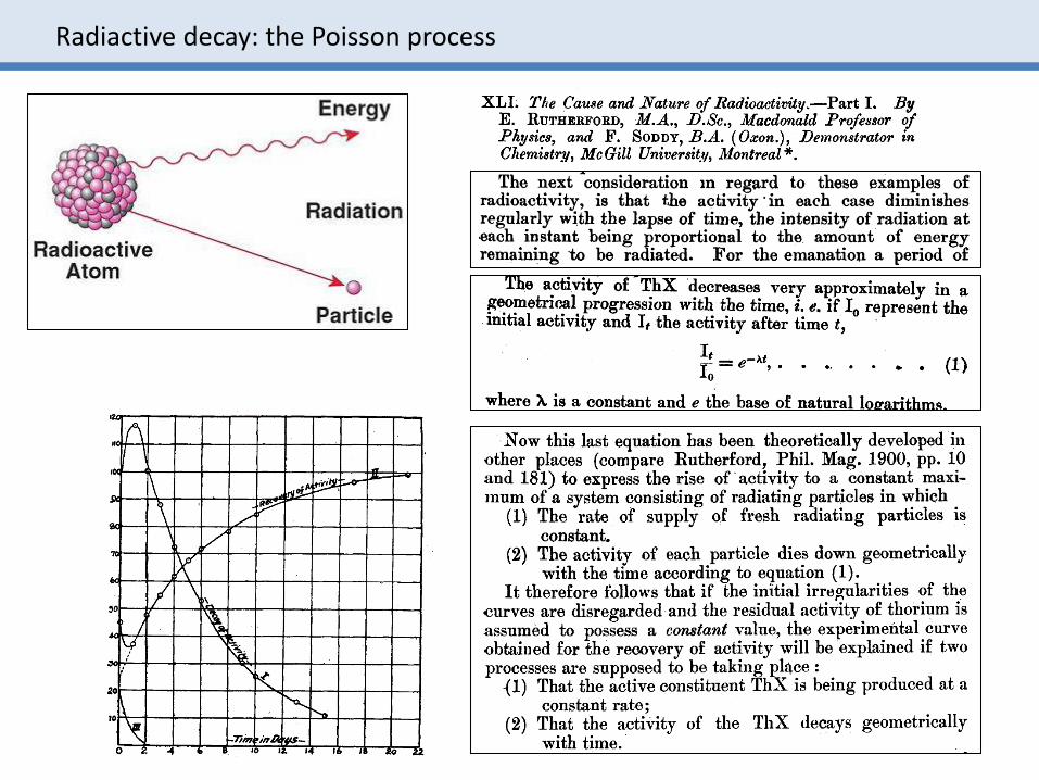
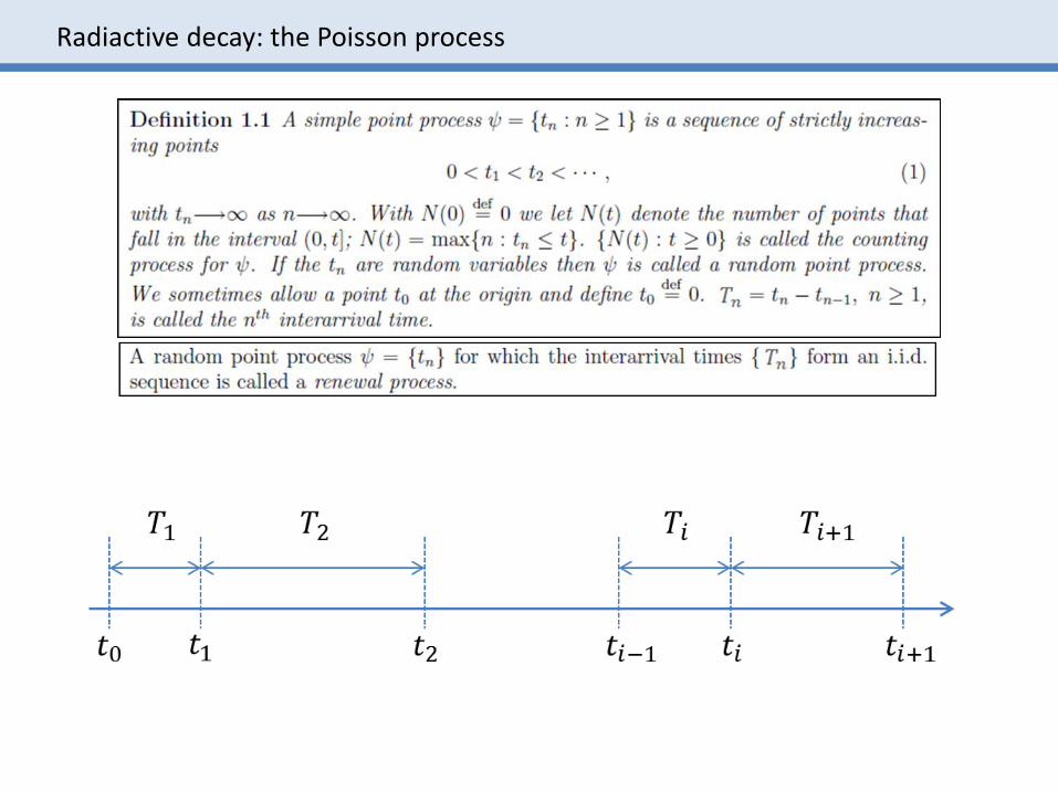
Radiactive decay: the Poisson process
Radiactive decay: the Poisson process
Radiactive decay: the Poisson process
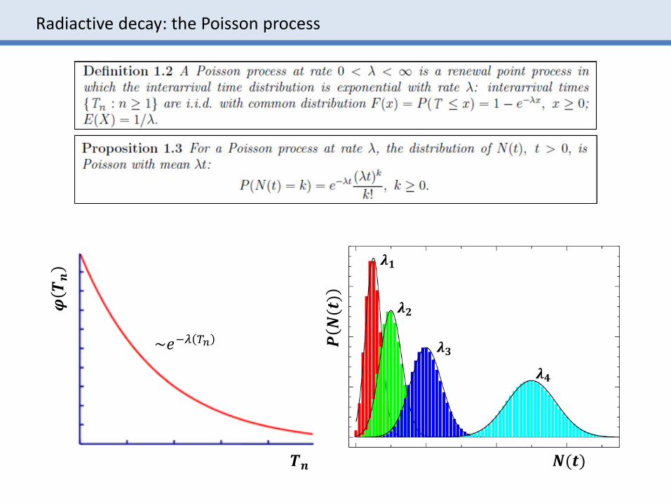
𝑻𝒏
𝝋𝑻𝒏
~𝑒−𝜆 𝑇𝑛 𝑷𝑵(𝒕)
𝑵(𝒕)
𝝀𝟏
𝝀𝟐
𝝀𝟑
𝝀𝟒
Radiactive decay: the Poisson process
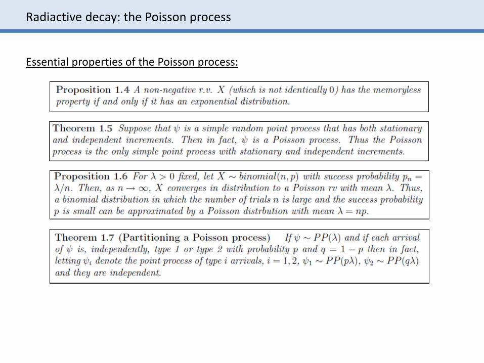
Essential properties of the Poisson process:
Radiactive decay: the Poisson process
Radiactive decay: the Poisson process
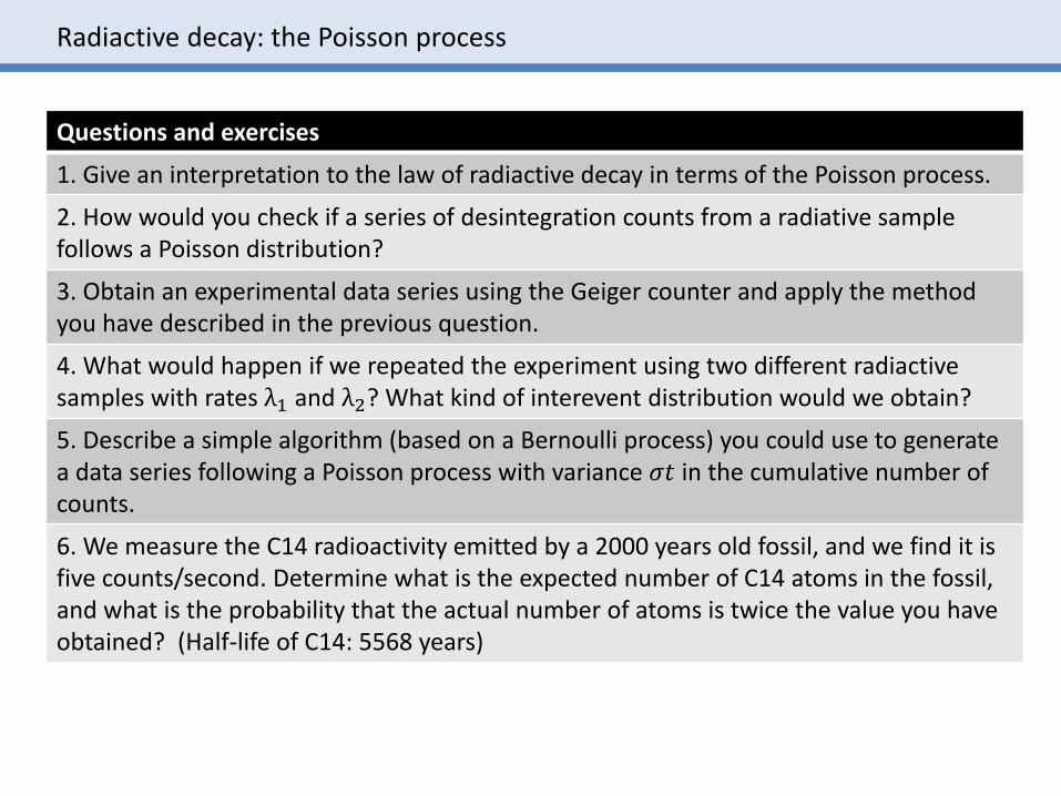
Questions and exercises
1. Give an interpretation to the law of radiactive decay in terms of the Poisson process.
2. How would you check if a series of desintegration counts from a radiative samplefollows a Poisson distribution?
3. Obtain an experimental data series using the Geiger counter and apply the methodyou have described in the previous question.
4. What would happen if we repeated the experiment using two different radiactivesamples with rates λ1 and λ2? What kind of interevent distribution would we obtain?
5. Describe a simple algorithm (based on a Bernoulli process) you could use to generatea data series following a Poisson process with variance 𝜎𝑡 in the cumulative number of counts.
6. We measure the C14 radioactivity emitted by a 2000 years old fossil, and we find it isfive counts/second. Determine what is the expected number of C14 atoms in the fossil,and what is the probability that the actual number of atoms is twice the value you haveobtained? (Half-life of C14: 5568 years)

2. CHEMICAL KINETICSSTOCHASTIC SIMULATION
Chemical kinetics: stochastic simulation
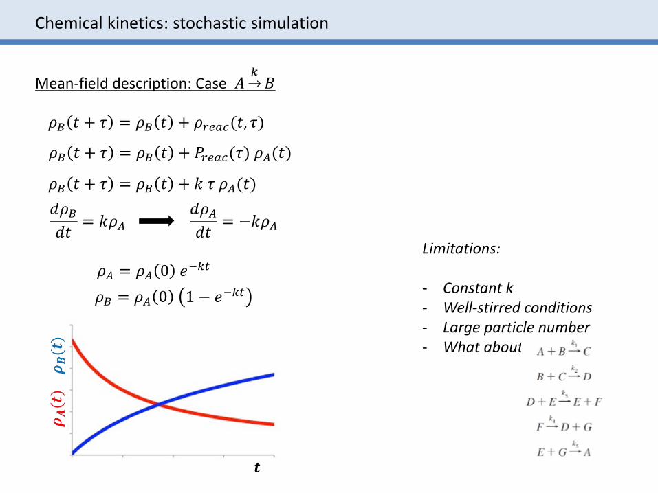
Mean-field description: Case 𝐴՜𝑘𝐵
𝜌𝐵 𝑡 + 𝜏 = 𝜌𝐵 𝑡 + 𝜌𝑟𝑒𝑎𝑐(𝑡, 𝜏)
𝜌𝐵 𝑡 + 𝜏 = 𝜌𝐵 𝑡 + 𝑃𝑟𝑒𝑎𝑐(𝜏) 𝜌𝐴(𝑡)
𝜌𝐵 𝑡 + 𝜏 = 𝜌𝐵 𝑡 + 𝑘 𝜏 𝜌𝐴(𝑡)
𝑑𝜌𝐵𝑑𝑡
= 𝑘𝜌𝐴𝑑𝜌𝐴𝑑𝑡
= −𝑘𝜌𝐴
𝜌𝐴 = 𝜌𝐴 0 𝑒−𝑘𝑡
𝜌𝐵 = 𝜌𝐴 0 1 − 𝑒−𝑘𝑡
Limitations:
- Constant k- Well-stirred conditions- Large particle number- What about
Chemical kinetics: stochastic simulation
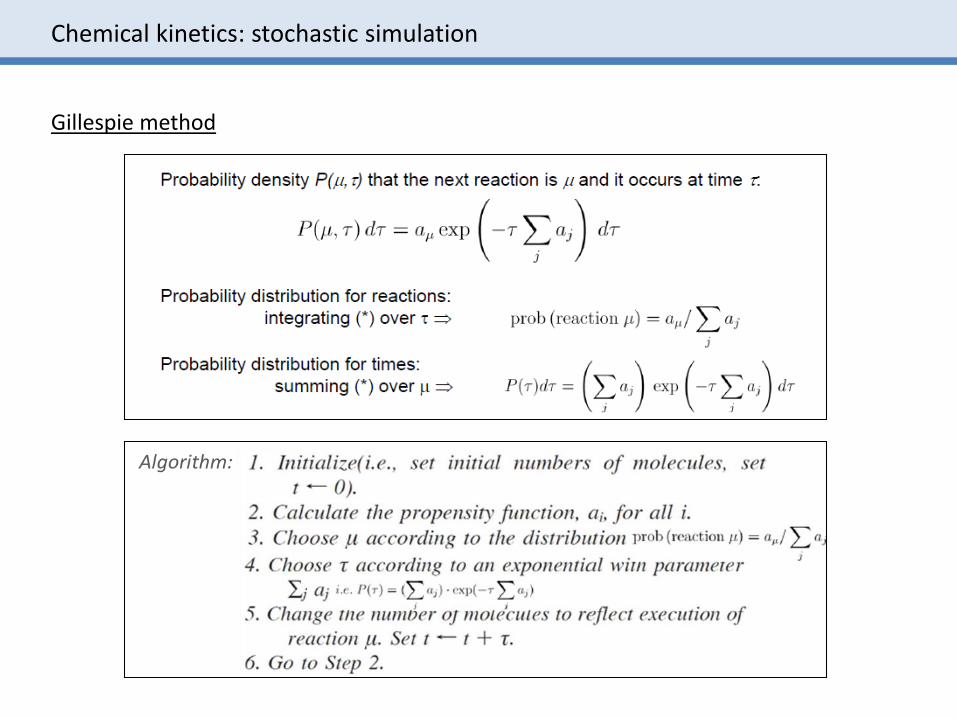
Gillespie method
Chemical kinetics: stochastic simulation
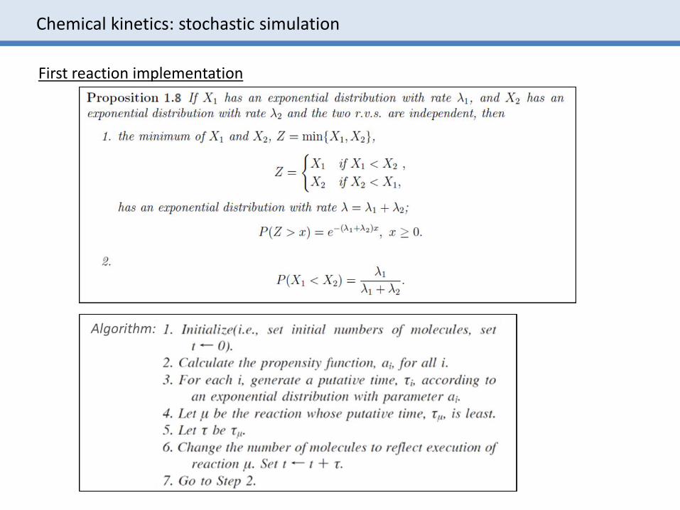
First reaction implementation
Chemical kinetics: stochastic simulation
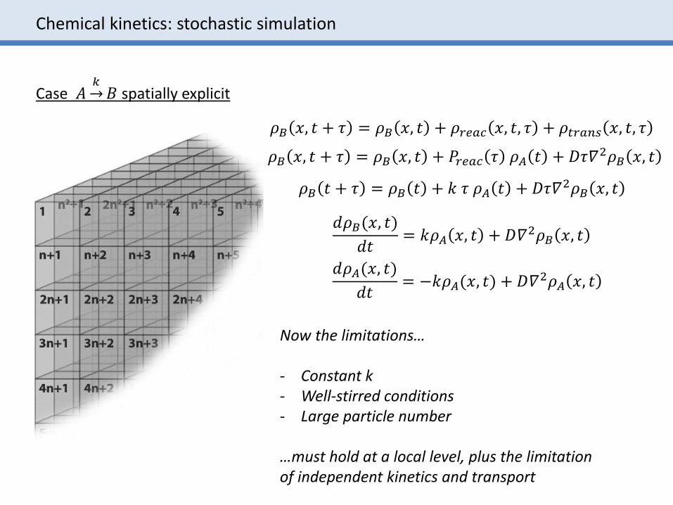
Case 𝐴՜𝑘𝐵 spatially explicit
Now the limitations…
- Constant k- Well-stirred conditions- Large particle number
…must hold at a local level, plus the limitationof independent kinetics and transport
𝜌𝐵 𝑥, 𝑡 + 𝜏 = 𝜌𝐵 𝑥, 𝑡 + 𝜌𝑟𝑒𝑎𝑐 𝑥, 𝑡, 𝜏 + 𝜌𝑡𝑟𝑎𝑛𝑠 𝑥, 𝑡, 𝜏
𝜌𝐵 𝑥, 𝑡 + 𝜏 = 𝜌𝐵 𝑥, 𝑡 + 𝑃𝑟𝑒𝑎𝑐 𝜏 𝜌𝐴 𝑡 + 𝐷𝜏𝛻2𝜌𝐵 𝑥, 𝑡
𝜌𝐵 𝑡 + 𝜏 = 𝜌𝐵 𝑡 + 𝑘 𝜏 𝜌𝐴 𝑡 + 𝐷𝜏𝛻2𝜌𝐵 𝑥, 𝑡
𝑑𝜌𝐵(𝑥, 𝑡)
𝑑𝑡= 𝑘𝜌𝐴 𝑥, 𝑡 + 𝐷𝛻2𝜌𝐵 𝑥, 𝑡
𝑑𝜌𝐴(𝑥, 𝑡)
𝑑𝑡= −𝑘𝜌𝐴(𝑥, 𝑡) + 𝐷𝛻2𝜌𝐴 𝑥, 𝑡
Chemical kinetics: stochastic simulation
Questions and exercises
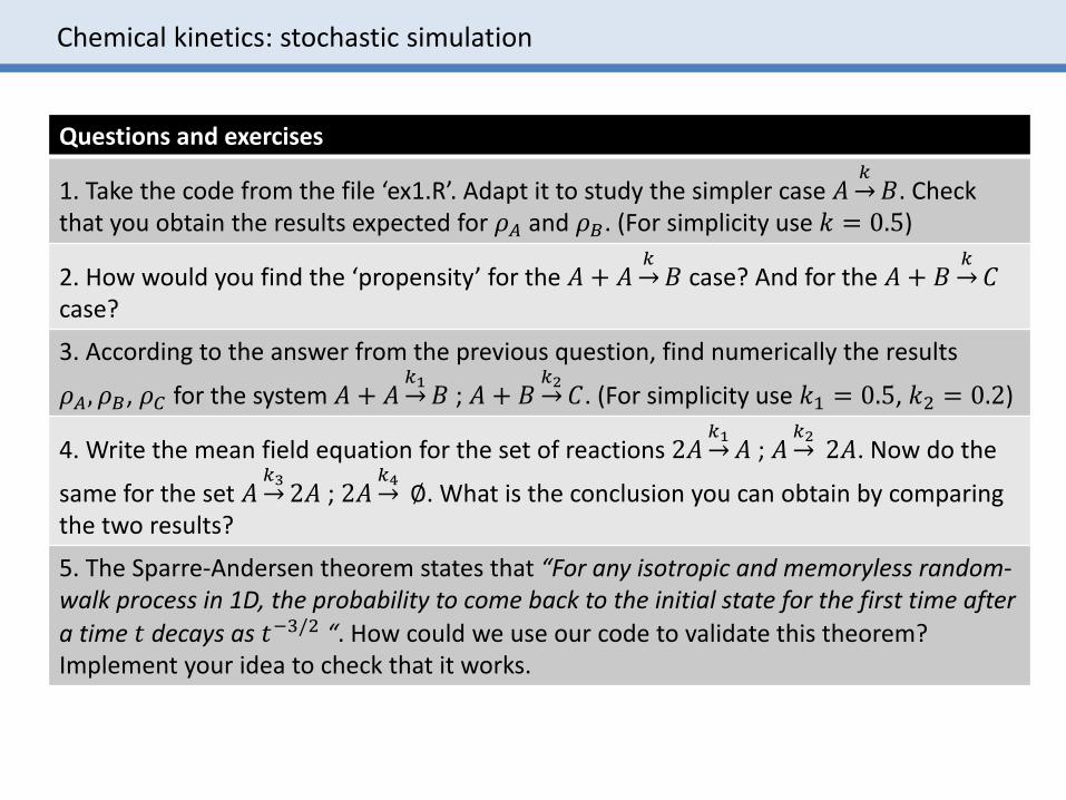
1. Take the code from the file ‘ex1.R’. Adapt it to study the simpler case 𝐴՜𝑘𝐵. Check
that you obtain the results expected for 𝜌𝐴 and 𝜌𝐵. (For simplicity use 𝑘 = 0.5)
2. How would you find the ‘propensity’ for the 𝐴 + 𝐴՜𝑘𝐵 case? And for the 𝐴 + 𝐵՜
𝑘𝐶
case?
3. According to the answer from the previous question, find numerically the results
𝜌𝐴, 𝜌𝐵, 𝜌𝐶 for the system 𝐴 + 𝐴՜𝑘1𝐵 ; 𝐴 + 𝐵՜
𝑘2𝐶. (For simplicity use 𝑘1 = 0.5, 𝑘2 = 0.2)
4. Write the mean field equation for the set of reactions 2𝐴՜𝑘1𝐴 ; 𝐴՜
𝑘22𝐴. Now do the
same for the set 𝐴՜𝑘32𝐴 ; 2𝐴՜
𝑘4∅. What is the conclusion you can obtain by comparing
the two results?
5. The Sparre-Andersen theorem states that “For any isotropic and memoryless random-walk process in 1D, the probability to come back to the initial state for the first time after
a time 𝑡 decays as 𝑡−3/2 “. How could we use our code to validate this theorem? Implement your idea to check that it works.
3. ECONOPHYSICSTHE RANDOM-WALK HYPOTHESIS
Econophysics: the Random-Walk hypothesis
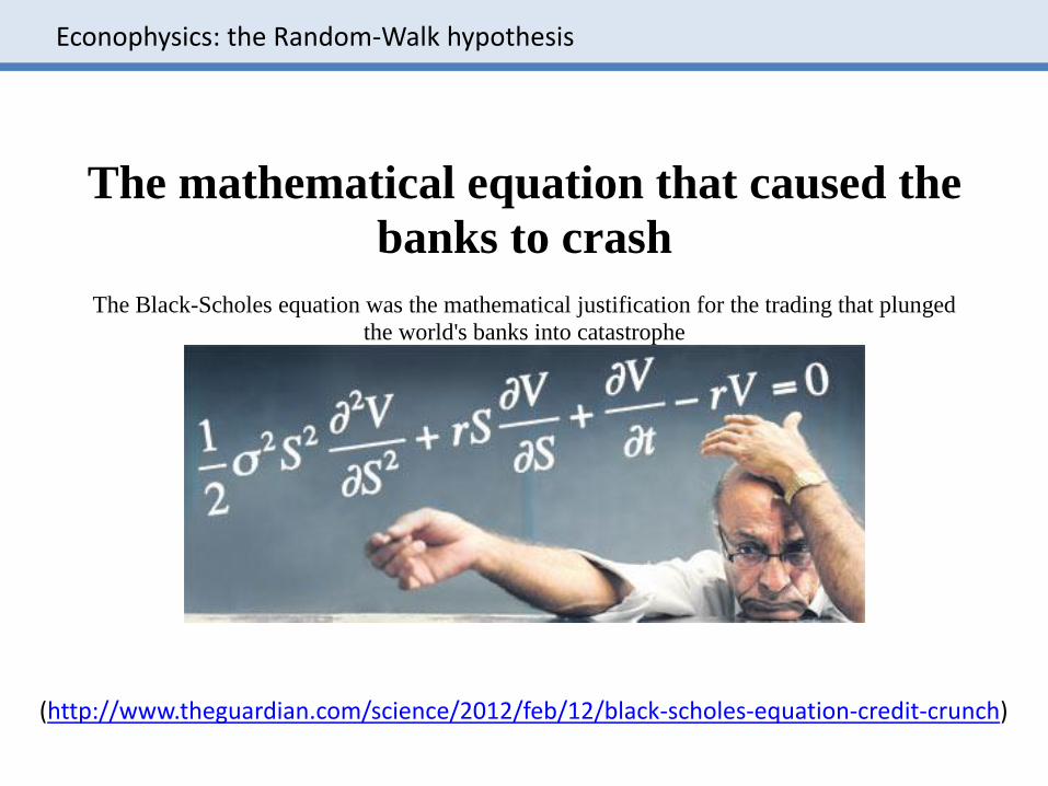
The mathematical equation that caused the
banks to crash
The Black-Scholes equation was the mathematical justification for the trading that plunged
the world's banks into catastrophe
(http://www.theguardian.com/science/2012/feb/12/black-scholes-equation-credit-crunch)
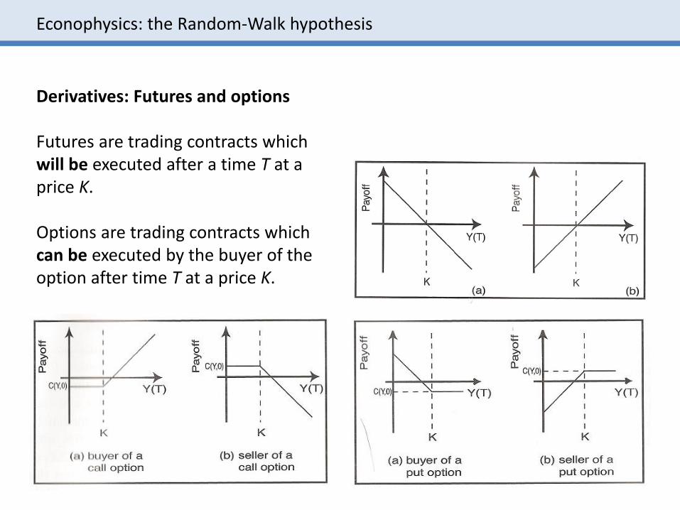
Derivatives: Futures and options
Futures are trading contracts whichwill be executed after a time T at a price K.
Options are trading contracts whichcan be executed by the buyer of theoption after time T at a price K.
Econophysics: the Random-Walk hypothesis
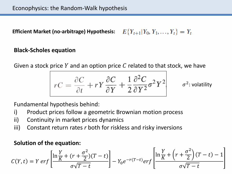
Black-Scholes equation
Given a stock price 𝑌 and an option price 𝐶 related to that stock, we have
Fundamental hypothesis behind: i) Product prices follow a geometric Brownian motion processii) Continuity in market prices dynamicsiii) Constant return rates r both for riskless and risky inversions
Solution of the equation:
𝐶 𝑌, 𝑡 = 𝑌 𝑒𝑟𝑓ln𝑌𝐾+ (𝑟 +
𝜎2
2)(𝑇 − 𝑡)
𝜎 𝑇 − 𝑡− 𝑌0𝑒
−𝑟(𝑇−𝑡)𝑒𝑟𝑓ln𝑌𝐾+ 𝑟 +
𝜎2
2𝑇 − 𝑡 − 1
𝜎 𝑇 − 𝑡
Econophysics: the Random-Walk hypothesis
𝜎2: volatility
Efficient Market (no-arbitrage) Hypothesis:
Econophysics: the Random-Walk hypothesis
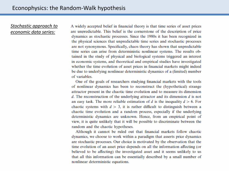
Stochastic approach to economic data series:
Econophysics: the Random-Walk hypothesis
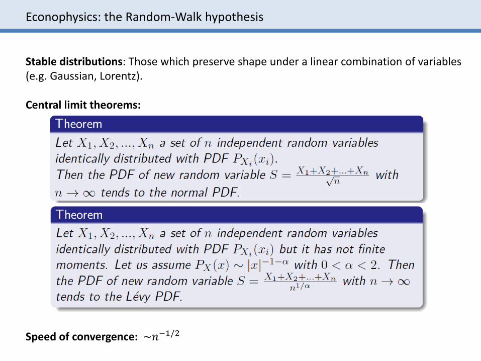
Stable distributions: Those which preserve shape under a linear combination of variables (e.g. Gaussian, Lorentz).
Central limit theorems:
Speed of convergence: ~𝑛−1/2
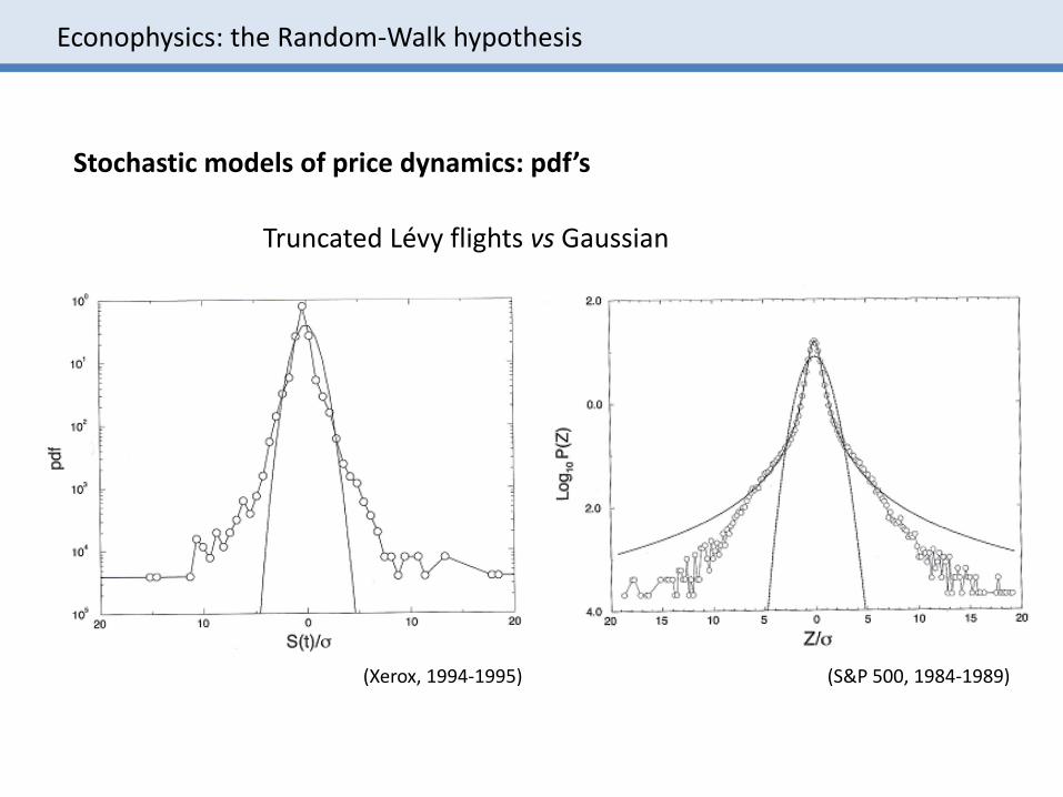
Stochastic models of price dynamics: pdf’s
Truncated Lévy flights vs Gaussian
(Xerox, 1994-1995) (S&P 500, 1984-1989)
Econophysics: the Random-Walk hypothesis
Econophysics: the Random-Walk hypothesis
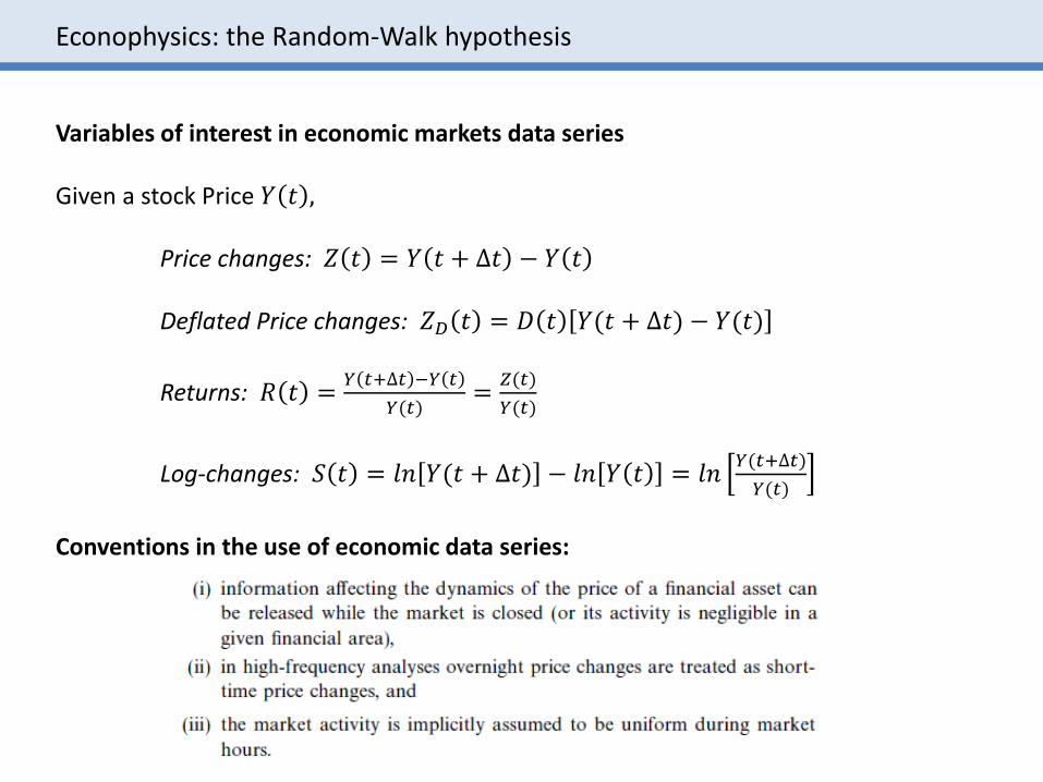
Variables of interest in economic markets data series
Given a stock Price 𝑌 𝑡 ,
Price changes: 𝑍 𝑡 = 𝑌 𝑡 + ∆𝑡 − 𝑌 𝑡
Deflated Price changes: 𝑍𝐷 𝑡 = 𝐷 𝑡 𝑌(𝑡 + ∆𝑡) − 𝑌(𝑡)
Returns: 𝑅 𝑡 =𝑌 𝑡+∆𝑡 −𝑌 𝑡
𝑌(𝑡)=
𝑍(𝑡)
𝑌(𝑡)
Log-changes: 𝑆 𝑡 = 𝑙𝑛 𝑌(𝑡 + ∆𝑡) − 𝑙𝑛 𝑌 𝑡 = 𝑙𝑛𝑌(𝑡+∆𝑡)
𝑌(𝑡)
Conventions in the use of economic data series:
Econophysics: the Random-Walk hypothesis
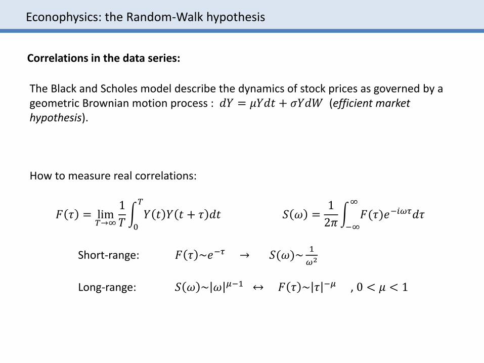
Correlations in the data series:
The Black and Scholes model describe the dynamics of stock prices as governed by a geometric Brownian motion process : 𝑑𝑌 = 𝜇𝑌𝑑𝑡 + 𝜎𝑌𝑑𝑊 (efficient markethypothesis).
How to measure real correlations:
𝐹 𝜏 = lim𝑇՜∞
1
𝑇න0
𝑇
𝑌 𝑡 𝑌 𝑡 + 𝜏 𝑑𝑡 𝑆 𝜔 =1
2𝜋න−∞
∞
𝐹(𝜏)𝑒−𝑖𝜔𝜏𝑑𝜏
Short-range: 𝐹 𝜏 ~𝑒−𝜏 ՜ 𝑆(𝜔)~1
𝜔2
Long-range: 𝑆 𝜔 ~ 𝜔 𝜇−1 ↔ 𝐹 𝜏 ~ 𝜏 −𝜇 , 0 < 𝜇 < 1
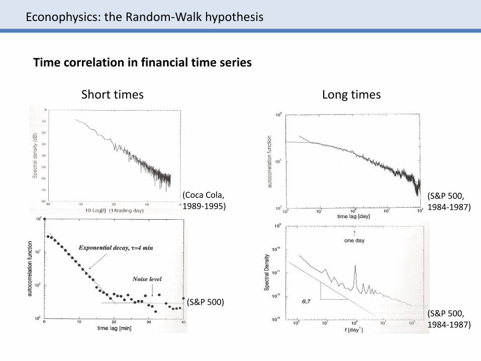
Time correlation in financial time series
Short times Long times
(Coca Cola, 1989-1995)
(S&P 500)
(S&P 500, 1984-1987)
(S&P 500, 1984-1987)
Econophysics: the Random-Walk hypothesis
Econophysics: the Random-Walk hypothesis
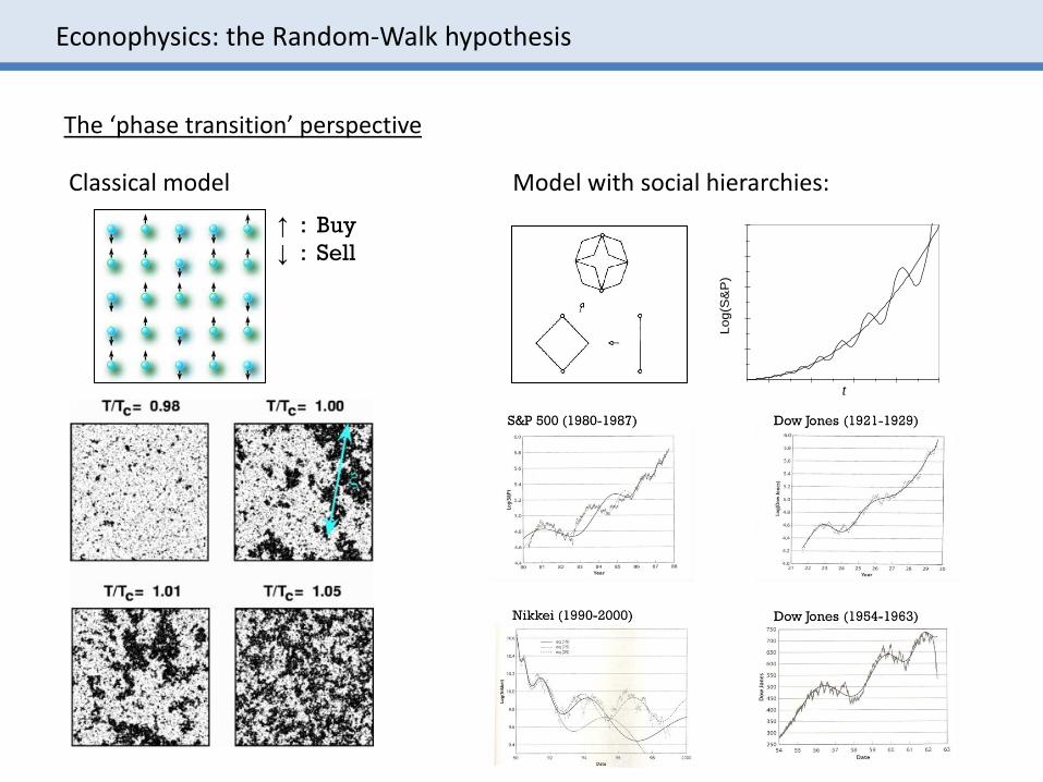
The ‘phase transition’ perspective
↑ : Buy
↓ : Sell
Classical model Model with social hierarchies:
Lo
g(S
&P
)
t
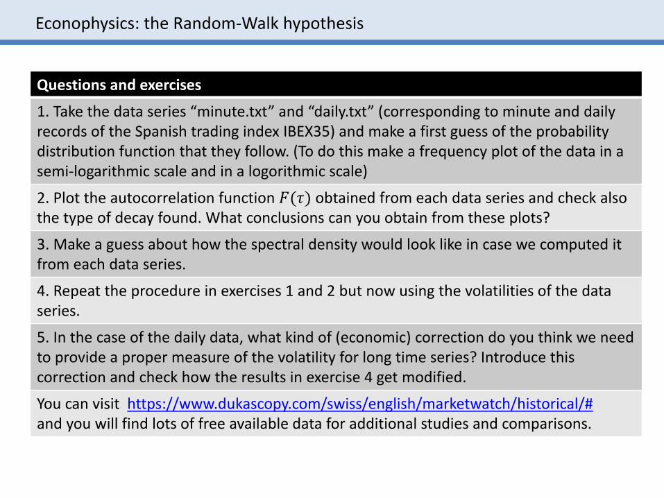
Questions and exercises
1. Take the data series “minute.txt” and “daily.txt” (corresponding to minute and dailyrecords of the Spanish trading index IBEX35) and make a first guess of the probabilitydistribution function that they follow. (To do this make a frequency plot of the data in a semi-logarithmic scale and in a logorithmic scale)
2. Plot the autocorrelation function 𝐹(𝜏) obtained from each data series and check alsothe type of decay found. What conclusions can you obtain from these plots?
3. Make a guess about how the spectral density would look like in case we computed itfrom each data series.
4. Repeat the procedure in exercises 1 and 2 but now using the volatilities of the data series.
5. In the case of the daily data, what kind of (economic) correction do you think we needto provide a proper measure of the volatility for long time series? Introduce thiscorrection and check how the results in exercise 4 get modified.
You can visit https://www.dukascopy.com/swiss/english/marketwatch/historical/#and you will find lots of free available data for additional studies and comparisons.
Econophysics: the Random-Walk hypothesis
4. EYE-TRACKINGCONTINUOUS-TIME RANDOM-WALKS
Eye-tracking: Continuous-Time Random Walks
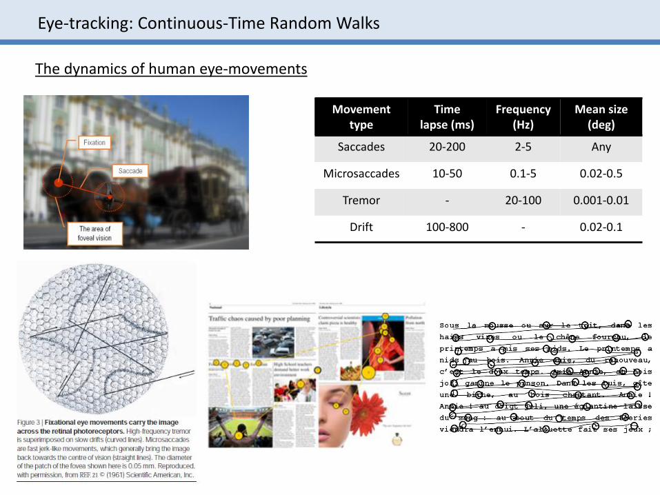
Movementtype
Timelapse (ms)
Frequency(Hz)
Mean size(deg)
Saccades 20-200 2-5 Any
Microsaccades 10-50 0.1-5 0.02-0.5
Tremor - 20-100 0.001-0.01
Drift 100-800 - 0.02-0.1
The dynamics of human eye-movements
Eye-tracking: Continuous-Time Random Walks
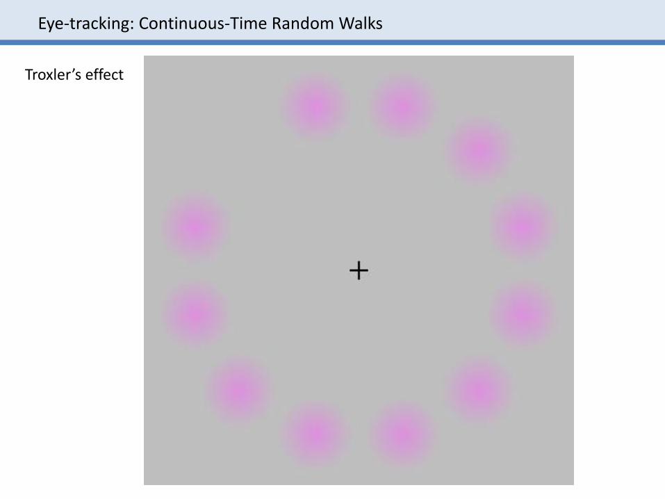
Troxler’s effect
Eye-tracking: Continuous-Time Random Walks
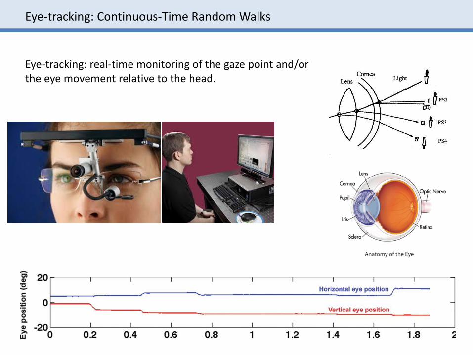
Eye-tracking: real-time monitoring of the gaze point and/orthe eye movement relative to the head.
Eye-tracking: Continuous-Time Random Walks
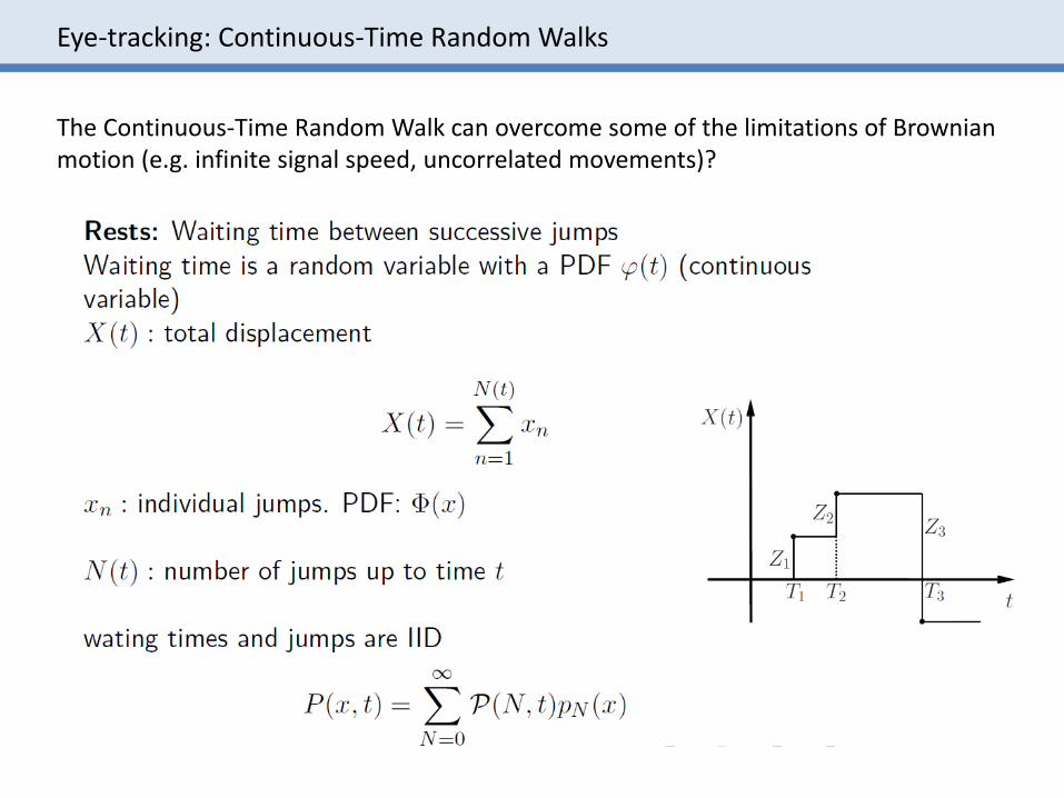
The Continuous-Time Random Walk can overcome some of the limitations of Brownianmotion (e.g. infinite signal speed, uncorrelated movements)?
Eye-tracking: Continuous-Time Random Walks
Eye-tracking: Continuous-Time Random Walks
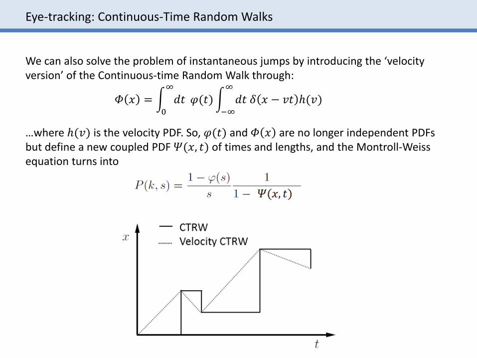
We can also solve the problem of instantaneous jumps by introducing the ‘velocityversion’ of the Continuous-time Random Walk through:
…where ℎ(𝑣) is the velocity PDF. So, 𝜑(𝑡) and 𝛷 𝑥 are no longer independent PDFsbut define a new coupled PDF 𝛹(𝑥, 𝑡) of times and lengths, and the Montroll-Weissequation turns into
𝛷 𝑥 = න0
∞
𝑑𝑡 𝜑(𝑡)න−∞
∞
𝑑𝑡 𝛿 𝑥 − 𝑣𝑡 ℎ(𝑣)
Questions and exercises
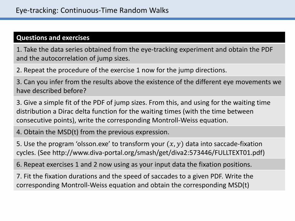
1. Take the data series obtained from the eye-tracking experiment and obtain the PDF and the autocorrelation of jump sizes.
2. Repeat the procedure of the exercise 1 now for the jump directions.
3. Can you infer from the results above the existence of the different eye movements wehave described before?
3. Give a simple fit of the PDF of jump sizes. From this, and using for the waiting time distribution a Dirac delta function for the waiting times (with the time betweenconsecutive points), write the corresponding Montroll-Weiss equation.
4. Obtain the MSD(t) from the previous expression.
5. Use the program ‘olsson.exe’ to transform your (𝑥, 𝑦) data into saccade-fixationcycles. (See http://www.diva-portal.org/smash/get/diva2:573446/FULLTEXT01.pdf)
6. Repeat exercises 1 and 2 now using as your input data the fixation positions.
7. Fit the fixation durations and the speed of saccades to a given PDF. Write thecorresponding Montroll-Weiss equation and obtain the corresponding MSD(t)
Eye-tracking: Continuous-Time Random Walks

5. SEARCH GAMESFIRST-PASSAGE PROCESSES
Search games: first-passage processes
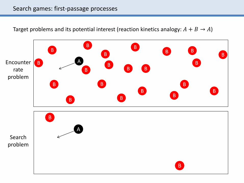
Target problems and its potential interest (reaction kinetics analogy: 𝐴 + 𝐵 ՜ 𝐴)
Encounterrate
problem
Searchproblem
Search games: first-passage processes
A
B
B
B
B
BB
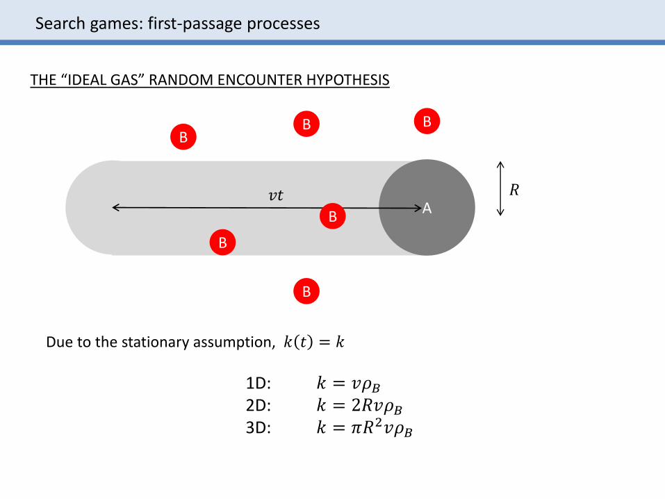
THE “IDEAL GAS” RANDOM ENCOUNTER HYPOTHESIS
Due to the stationary assumption, 𝑘 𝑡 = 𝑘
1D: 𝑘 = 𝑣𝜌𝐵2D: 𝑘 = 2𝑅𝑣𝜌𝐵3D: 𝑘 = 𝜋𝑅2𝑣𝜌𝐵
𝑅𝑣𝑡
Search games: first-passage processes
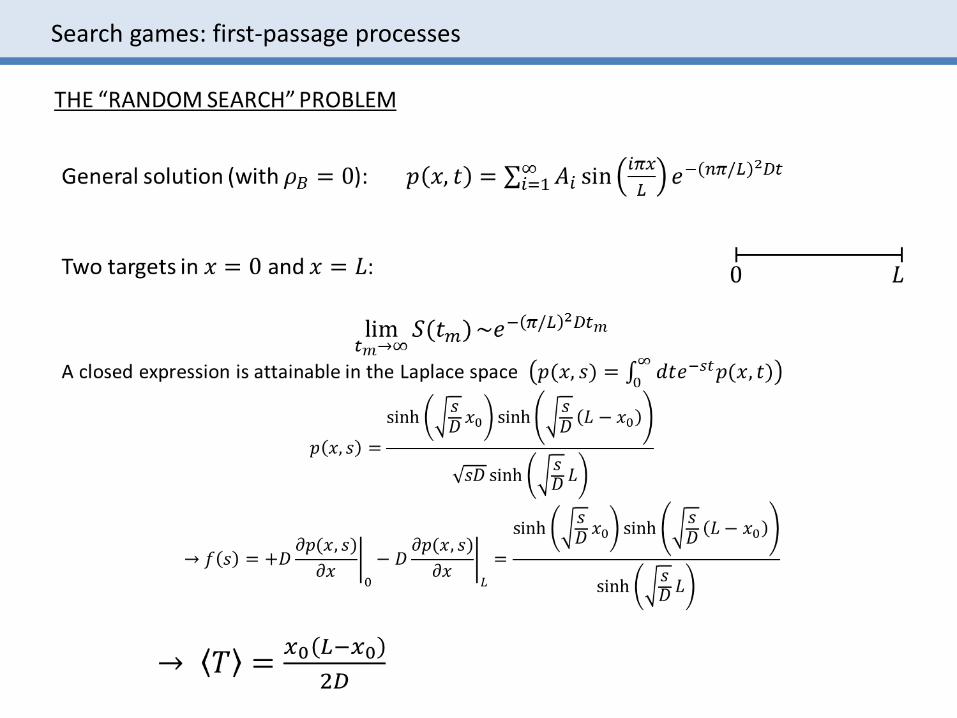
Search games: first-passage processes

Search games: first-passage processes
Search games: first-passage processes
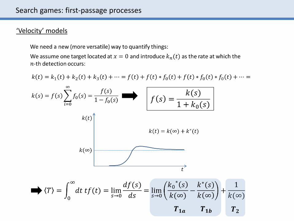
‘Velocity’ models
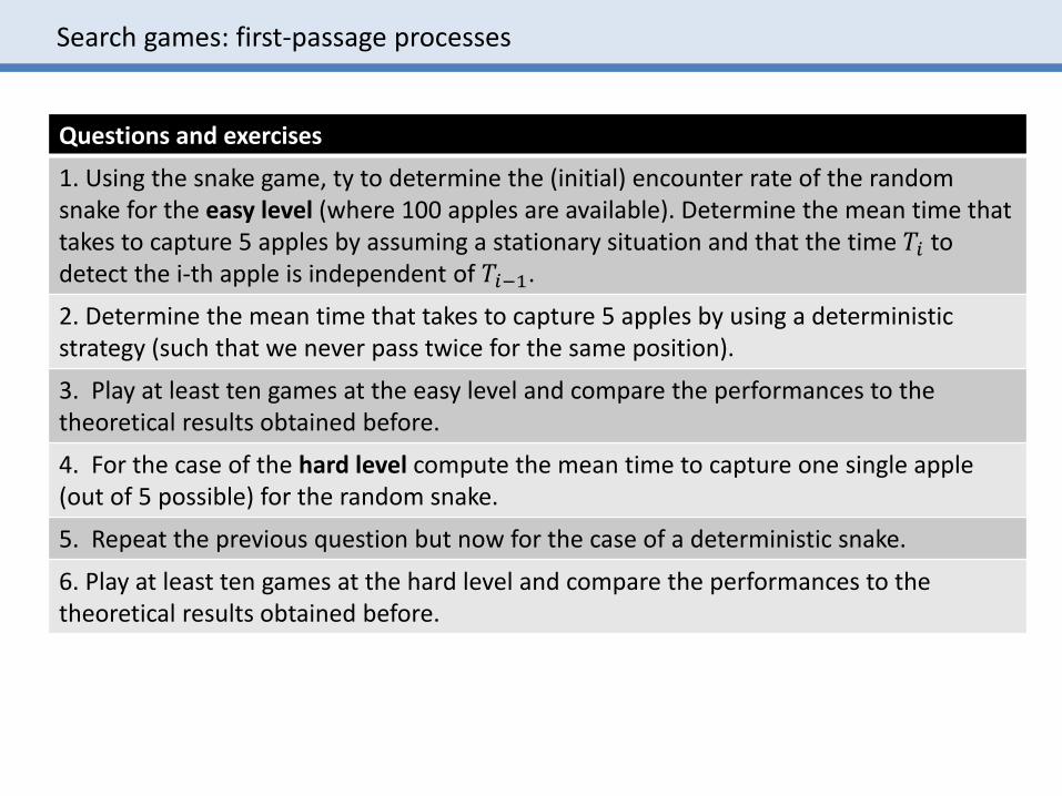
Questions and exercises
1. Using the snake game, ty to determine the (initial) encounter rate of the randomsnake for the easy level (where 100 apples are available). Determine the mean time thattakes to capture 5 apples by assuming a stationary situation and that the time 𝑇𝑖 todetect the i-th apple is independent of 𝑇𝑖−1.
2. Determine the mean time that takes to capture 5 apples by using a deterministicstrategy (such that we never pass twice for the same position).
3. Play at least ten games at the easy level and compare the performances to thetheoretical results obtained before.
4. For the case of the hard level compute the mean time to capture one single apple(out of 5 possible) for the random snake.
5. Repeat the previous question but now for the case of a deterministic snake.
6. Play at least ten games at the hard level and compare the performances to thetheoretical results obtained before.
Search games: first-passage processes