applying root-locus techniques to the analysis of coupled modes
TRANSCRIPT
Timothy Stilson CCRMA Affiliates [email protected] http://www-ccrma.stanford.edu/~stilti
Applying Root-Locus Techniquesto the Analysis of Coupled Modes
in Piano Strings
• The Root-Locus Analysis Method
• Loaded N-Port Junction String Coupling
• 2-Mode Coupling
– Root-Locus– Compare with Weinreich, etc.
• 2-String Coupling
• 3-Mode Coupling
• 3-String Coupling
• Conclusion
Originally presented at the Conference of the Acoustical Society of America, Hawaii, 1996. Also to bepresented at the International Computer Music Conference, Greece, 1997
1

Root-Locus Analysis
G
Hk
Transfer Function:
G
1 +kGH
Poles:
1 +kGH = 0⇒GH =−1
kk real, k > 0
Let ND
=GH, so that:
D+kN = 0
• At k = 0, the system poles are at the poles of GH
• As k→∞, the system poles go to the zeros of GH
• The complete root locus: {s : 6 G(s)H(s) = π}
2

N-Port Junction String Coupling
Gload
An N-Port Junction
delay
delay
delay
delay
GloopGloadGloop
Coupled Strings
delay1 Gloop
delay2 Gloop
Gload
Rearranged to Root-Locus Form
3

N-Port Junction String Coupling
delay1 Gloop
delay2 Gloop
Gload
GForward
For simplicity, let Gloop(s) =−a, then:
GForward(s) = Σn
−ae−sTn
1−ae−sTn
Poles of each term:
s =1
Tn(lna+ ikπ) for k = 0,±2,±4, . . .
Note that we do not define any input or output. Pole locationsare not affected by input/output choices. The ‘zeros’ we will talkabout are the zeros of the loop transfer function.
4
Zeros of Summed Poles
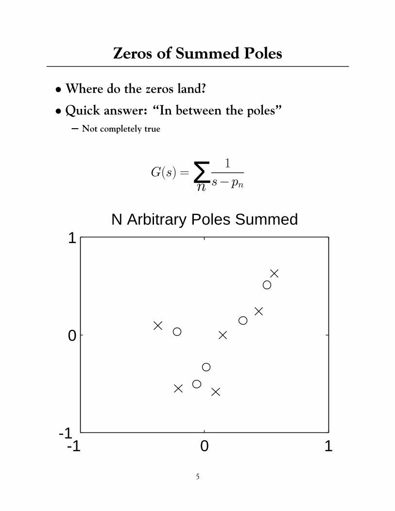
•Where do the zeros land?
• Quick answer: “In between the poles”– Not completely true
G(s) = Σn
1
s−pn
-1 0 1-1
0
1N Arbitrary Poles Summed
5

Zeros of Summed Poles, Phase Effects
• Extra phase in the poles (which happens in thestring case) moves the zero locations around.
G(s) = Σn
eiφn
s−pn
poles
zeros, poles have no extra phase
zeros, each pole also has a phase
-1 -0.5 0 0.5 1-1
0
1N Arbitrary Poles Summed, Extra Phase Effects
6

Zeros of Summed Poles, Strings
Summing two sets of poles: the zeros land between the poles.∑i
1
s−pi+∑i
1
s− qi
A single string is more like a product of its poles, so the sum oftwo strings has half the number of zeros:
1
1− e−sT1+
1
1− e−sT2≈
∏i
1
s−pi+∏i
1
s− qi
The phase of the strings moves the zeros:
−e−sT1
1− e−sT1+−e−sT2
1− e−sT2
7
Basic 2-Summed-Pole Root-LociRoot Loci in loop gain k
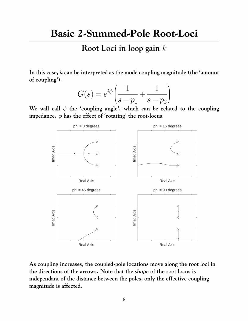
In this case, k can be interpreted as the mode coupling magnitude (the ‘amountof coupling’).
G(s) = eiφ 1
s−p1+
1
s−p2
We will call φ the ‘coupling angle’, which can be related to the couplingimpedance. φ has the effect of ‘rotating’ the root-locus.
Real Axis
Imag
Axi
s
phi = 0 degrees
Real Axis
Imag
Axi
s
phi = 15 degrees
Real Axis
Imag
Axi
s
phi = 45 degrees
Real Axis
Imag
Axi
s
phi = 90 degrees
As coupling increases, the coupled-pole locations move along the root loci inthe directions of the arrows. Note that the shape of the root locus isindependant of the distance between the poles, only the effective couplingmagnitude is affected.
8

Coupling Magnitude
We plot the Root-Locus on top of the magnitude of the looptransfer function (|GH|). The magnitude condition of theroot-locus (|GH|= 1
k) implies that the closed-loop poles will end
up at the intersection of the 6 (GH) = π and |GH| = 1/k
contours. Thus, the coupling magnitude k controls the characterof the coupling: at low coupling, the poles stay near theiropen-loop locations and beat against each other; at highcoupling, the poles go to similar frequencies, but with stronglydifferent decay rates (the ‘two-stage’ decay).
Root-Locus, with coupled-pole locationsfor a few values of coupling magnitude0-degree coupling
★
10-degree coupling
frequency
decayrate
The distance between the open-loop poles has a large effect onthe coupling: if the poles are close, the system will entertwo-stage decay at lower values of coupling magnitude. This willhave a large effect in detuned strings, where at low harmonics,the two strings’ harmonic poles are close, and at high harmonics,they are further apart. Thus, a given value of coupling can causetwo-stage decay at the low harmonics, but just cause beating atthe high harmonics.
9

Decay and Pole Location
Sum of two real poles:
-2 -1 0-1
0
1
0 5 10 1510
-1
100
101
102
Sum of complex poles:
-2 -1 08
10
12
0 5 10 1510
-2
10-1
100
101
Sum of rotated complex poles (like complex coupling):Note that the frequencies may beat together near crossover
-2 -1 07
8
9
10
0 5 10 1510
-2
10-1
100
101
Three poles (note the beating in the second stage):
-2 -1 08
10
12
0 5 10 1510
-2
10-1
100
101
11
}–.15 –.1 9.9 10 10.1
9.9
10
10.1
Moving Pole Frequency
0–degree coupling
–.15 –.1 9.9 10 10.1
9.9
10
10.1
11–degree coupling
Moving Pole Frequency
–.15 –.1 9.9 10 10.1
9.9
10
10.1
45–degree coupling
Moving Pole Frequency–.15 –.1 9.9 10 10.1
9.5
9.6
9.7
9.8
9.9
10
90–degree coupling
Moving Pole Frequency
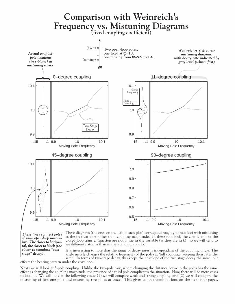
}Actual coupled-pole locations(in s-plane) as
mistuning varies.
Weinreich-stylefreq-vs-mistuning diagram,
with decay rate indicated bygray level (white: fast)
jω
(fixed)
(moving)
Two open-loop poles,one fixed at ω=10,one moving from ω=9.9 to 10.1
Comparison with Weinreich’sFrequency vs. Mistuning Diagrams
(fixed coupling coefficient)
MoreDamping
HigherFrequency
These diagrams (the ones on the left of each plot) correspond roughly to root-loci with mistuningas the free variable rather than coupling magnitude. In these root-loci, the coefficients of theclosed-loop transfer function are not affine in the variable (as they are in k), so we will tend tosee different patterns than in the ‘standard’ root loci.
It is interesting to note that the range of decay rates is independant of the coupling angle. Theangle merely changes the relative freqencies of the poles at ‘full coupling’, keeping their rates thesame. In terms of two-stage decay, this keeps the envelope of the two stage decay the same, but
effects the beating pattern under the envelope.
Next: we will look at 3-pole coupling. Unlike the two-pole case, where changing the distance between the poles has the sameeffect as changing the coupling magnitude, the presence of a third pole complicates the situation. Now, there will be more casesto look at. We will look at the following cases: (1) we will compare weak and strong coupling, and (2) we will compare themistuning of just one pole and mistuning two poles at once. This gives us four combinations on the next four pages.
Two-StageDecay
These lines connect polesof same open-loop mistun-ing. The closer to horizon-tal, the closer to black (thecloser to standard “two-stage” decay).
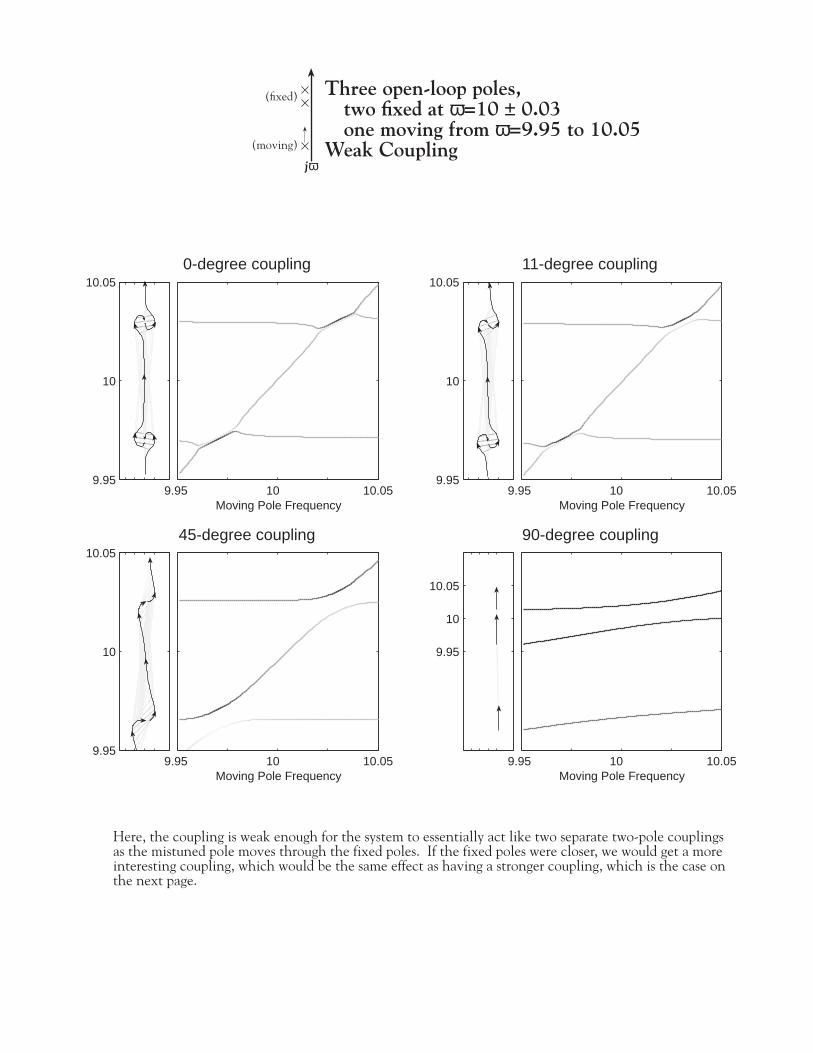
9.95 10 10.05Moving Pole Frequency
9.95
10
10.050-degree coupling
9.95 10 10.05Moving Pole Frequency
9.95
10
10.0511-degree coupling
9.95 10 10.05Moving Pole Frequency
9.95
10
10.0545-degree coupling
9.95 10 10.05Moving Pole Frequency
9.95
10
10.05
90-degree coupling
jω
(fixed)
(moving)
Three open-loop poles,two fixed at ω=10 ± 0.03one moving from ω=9.95 to 10.05
Weak Coupling
Here, the coupling is weak enough for the system to essentially act like two separate two-pole couplingsas the mistuned pole moves through the fixed poles. If the fixed poles were closer, we would get a moreinteresting coupling, which would be the same effect as having a stronger coupling, which is the case onthe next page.
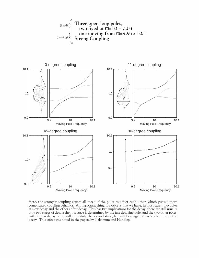
9.9 10 10.1Moving Pole Frequency
9.9
10
10.10-degree coupling
9.9 10 10.1Moving Pole Frequency
9.9
10
10.111-degree coupling
9.9 10 10.1Moving Pole Frequency
9.9
10
10.145-degree coupling
9.9 10 10.1Moving Pole Frequency
9.9
10
10.190-degree coupling
jω
(fixed)
(moving)
Three open-loop poles,two fixed at ω=10 ± 0.03one moving from ω=9.9 to 10.1
Strong Coupling
Here, the stronger coupling causes all three of the poles to affect each other, which gives a morecomplicated coupling behavior. An important thing to notice is that we have, in most cases, two polesat slow decay and the other at fast decay. This has two implications for the decay: there are still usuallyonly two stages of decay: the first stage is determined by the fast decaying pole, and the two other poles,with similar decay rates, will constitute the second stage, but will beat against each other during thedecay. This effect was noted in the papers by Nakamura and Hundley.

9.95 10 10.05Upper Moving Pole Frequency
9.95
10
10.050-degree coupling
9.95 10 10.05Upper Moving Pole Frequency
9.95
10
10.0545-degree coupling
9.95 10 10.05Upper Moving Pole Frequency
9.95
10
10.05
90-degree coupling
Three open-loop poles,one fixed at ω=10two moving from ω=9.95 & 9.92 to 10.05 & 10.02
Weak Couplingjω
(fixed)
(moving)
9.95 10 10.05Upper Moving Pole Frequency
9.95
10
10.0511-degree coupling
Here we get essintially the same effects as in the previous weak-coupling figure (2 pages back), but thetwo-pole couplings occur in the same frequency ranges, making the s-plane figures more complicated.We can see in the Weinreich diagrams, though, that the couplings are still mostly unaffected by eachother.

9.9 10 10.1Upper Moving Pole Frequency
9.9
10
10.1
0-degree coupling
9.9 10 10.1Upper Moving Pole Frequency
9.9
10
10.1
11-degree coupling
9.9 10 10.1Upper Moving Pole Frequency
9.9
10
10.1
45-degree coupling
9.9 10 10.1Upper Moving Pole Frequency
9.9
10
10.190-degree coupling
Three open-loop poles,one fixed at ω=10two moving from ω=9.9 & 9.87 to 10.1 & 10.07
Strong Couplingjω
(fixed)
(moving)
If we compare this case to the previous strong-coupling case (two pages back), the major difference isthat the poles are much closer to each other at their closest approach, which has the effect of makingthe coupling even stronger. Thus the fast-decay pole is further out to the left than before, and in thiscase the two moving poles have partially coupled together, so that even when they are far from the fixedpole, the fast pole stays at a quick decay.
The“Fast Pole”
These two poles would couple anyway, so aremoving to a two-stage position as they moveaway from the fixed pole. The fixed pole stillaffects the angle of their coupling, though.
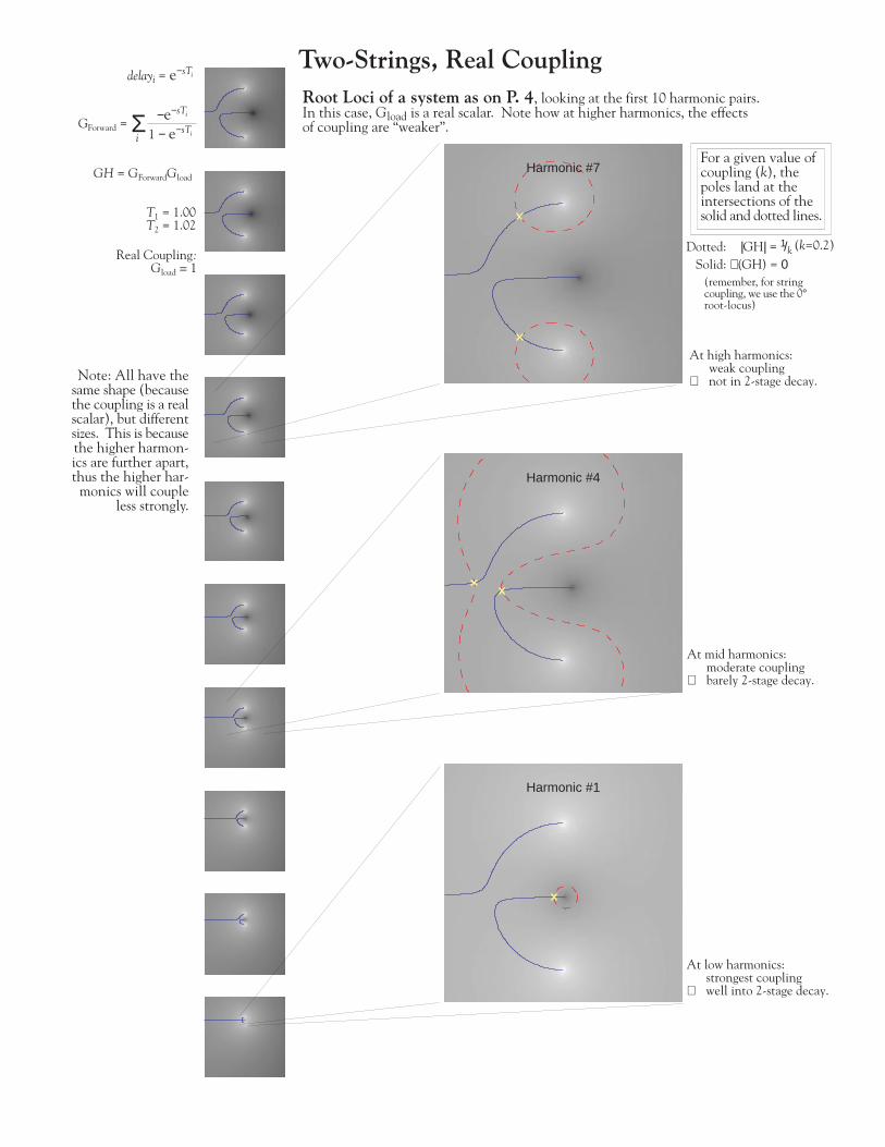
Harmonic #1
Harmonic #4
Harmonic #7
Two-Strings, Real Coupling
Note: All have thesame shape (becausethe coupling is a realscalar), but differentsizes. This is becausethe higher harmon-ics are further apart,thus the higher har-
monics will coupleless strongly.
Solid: ∠(GH) = 0Dotted: |GH| = 1/k (k=0.2)
At high harmonics: weak coupling⇒ not in 2-stage decay.
At mid harmonics: moderate coupling⇒ barely 2-stage decay.
At low harmonics: strongest coupling⇒ well into 2-stage decay.
delayi = e−sTi
GForward = −e−sTi
1 − e−sTiΣ
GH = GForwardGload
T1 = 1.00T2 = 1.02
Real Coupling:Gload = 1
Root Loci of a system as on P. 4, looking at the first 10 harmonic pairs.In this case, Gload is a real scalar. Note how at higher harmonics, the effectsof coupling are “weaker”.
i
For a given value ofcoupling (k), thepoles land at theintersections of thesolid and dotted lines.
(remember, for stringcoupling, we use the 0°root-locus)

Harmonic #1
Harmonic #4
Harmonic #7
Two-Strings, 1-Pole Coupling
At low frequencies, thecoupling filter has a
phase of essentially 0°(i.e. real). The couplingphase approaches 90° at
high harmonics, withcorrespondingly different
coupling behaviors.Solid: ∠(GH) = 0
Dotted: |GH| = 1/k (k=0.2)
In this case, Gload is a one-pole filter. This causes the coupling to be frequencydependant. i.e., each harmonic has a different coupling behavior.
For a given value ofcoupling (k), thepoles land at theintersections of thesolid and dotted lines.
(remember, for stringcoupling, we use the 0°root-locus)
One-Pole Coupling:
Gload =100
s+100
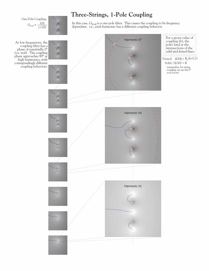
Harmonic #1
Harmonic #4
Harmonic #7
Three-Strings, 1-Pole Coupling
At low frequencies, thecoupling filter has a
phase of essentially 0°(i.e. real). The couplingphase approaches 90° at
high harmonics, withcorrespondingly different
coupling behaviors.Solid: ∠(GH) = 0
Dotted: |GH| = 1/k (k=0.2)
In this case, Gload is a one-pole filter. This causes the coupling to be frequencydependant. i.e., each harmonic has a different coupling behavior.
For a given value ofcoupling (k), thepoles land at theintersections of thesolid and dotted lines.
(remember, for stringcoupling, we use the 0°root-locus)
One-Pole Coupling:
Gload =100
s+100

Harmonic #1
Harmonic #4
Harmonic #7
Three-Strings, 1-Pole Coupling, with Damping
Solid: ∠(GH) = 0Dotted: |GH| = 1/k (k=0.2)
In this case,The strings also have damping, which moves their poles off the jω axis.This case also has a different detuning configuration than the previous figure.
For a given value ofcoupling (k), thepoles land at theintersections of thesolid and dotted lines.
(remember, for stringcoupling, we use the 0°root-locus)
One-Pole Coupling:
Gload =100
s+100

Note: There are 12 zeros, so all but one pole stay ‘near’ their open-loop positions (‘slow decay’),and the other pole goes out to the left (‘fast decay’).
White: Constant-Magnitude Contour,The closed-loop poles for a certain loop gainwill land at the intersections of the root-locus(blue) and this contour.
Root-Locus of 13 summedrandom single-poles
GForward = 1
s − piΣi
}
Conclusions
• The Root Locus Provides Intuition on CouplingBehavior
• In 3-Mode Coupling, Two Modes Stay at SlowDecays– This Gives the Beating in the Second Stage
• Different String Harmonics Couple Differently– Higher Harmonics are More Detuned (Absolute Detuning, Not
Relative).This Makes the Higher Harmonics “Less Coupled”.
– Frequency-Dependent Coupling Causes each Harmonic to CoupleDifferentlyEach Harmonic Couples with a Different Coupling Phase Angle.
References
[1] Weinreich, G. 1977. “Coupled Piano Strings”, J. Acoust. Soc. Am.Vol. 62, No. 6, pp. 1474-84.
[2] Hundley, C. et al 1978. “Factors Contributing to the Multiple Rate ofPiano Tone Decay”, J. Acoust. Soc. Am. Vol. 64, No. 4, pp. 1303-09.
[3] Nakamura, I. 1989. “Fundamental Theory and Computer simulation ofthe Decay Characteristics of Piano Sound”, J. Acoust. Soc. Jpn. Vol. 10,No. 5, pp. 289-97.
[4] Franklin, G., Powell, J.D., Emami-Naeini, A. 1994. Feedback Control ofDynamic Systems, New York: Addison-Wesley, pp. 243-336.
[5] Smith, J.O. 1993. “Efficient Synthesis of Stringed MusicalInstruments”, ICMC93, Tokyo, pp.64-71.
12