applying trajectory approach with static priority queuing for improving the use of available afdx...
TRANSCRIPT

Real-Time Syst (2012) 48:101–133DOI 10.1007/s11241-011-9142-9
Applying Trajectory approach with static priorityqueuing for improving the use of available AFDXresources
Henri Bauer · Jean-Luc Scharbarg ·Christian Fraboul
Published online: 1 December 2011© Springer Science+Business Media, LLC 2011
Abstract AFDX (Avionics Full Duplex Switched Ethernet) standardized as ARINC664 is a major upgrade for avionics systems. The mandatory certification implies aworst-case delay analysis of all the flows transmitted on the AFDX network. Up tonow, this analysis is done thanks to a tool based on a Network Calculus approach. Themore recent Trajectory approach has been proposed for the computation of worst-caseresponse time in distributed systems. It has been shown that the worst-case delay anal-ysis of an AFDX network can be improved using an optimized Trajectory approach.This paper extends this optimized approach with the integration of static priority QoSpolicies. This extension makes possible to compute the bounds needed for determin-istic avionics flows (high priority) when (lower priority) non avionics flows are added.Moreover, the paper provides an analysis of the pessimism of the obtained bounds.
Keywords Avionics networks · Worst-case delay analysis · AFDX · Trajectoryapproach
Notationsτi One flow on the networkPi Path of flow τi
hpi Set of flows having a fixed priority strictly higher than this of τi
spi Set of flows having a fixed priority equal to this of τi
lpi Set of flows having a fixed priority strictly lower than this of τi
Ti Minimum delay between two packets of τi
H. Bauer (�) · J.-L. Scharbarg · C. FraboulINP-ENSEEIHT and IRIT, Université de Toulouse, 2 rue Camichel, 31000 Toulouse, Francee-mail: [email protected]
J.-L. Scharbarge-mail: [email protected]
C. Fraboule-mail: [email protected]

102 Real-Time Syst (2012) 48:101–133
Ji Maximum release jitter of τi
Ci Transmission time of one packet of τi
Lmax Maximum switching delayaNh
m Arrival time of packet m in node Nh
bpNhBusy period of node Nh
f (Ni) First packet processed in bpNi
p(Ni−1) First packet processed in bpNiand coming from Ni−1
Ri Worst-case end-to-end response time of τi
Wlastii,t Latest starting time of a packet m generated at t on its last visited node
Ai,j Maximum relative jitter between τi and τj
Bi,j Maximum relative jitter between τi and τj
δhi Maximum non-preemption delay for τi on node h
ΔNhImpact of serialization on node Nh
1 Introduction
Designing and manufacturing new civilian aircraft has lead to an increase of the num-ber of embedded systems and functions. The AFDX (ARINC-664 2002–2005) bringsan answer by multiplexing a huge amount of communication flows over a full duplexswitched Ethernet network. It has become the reference communication technologyin the context of civilian avionics and provides a backbone network for the avionicsplatform.
Full duplex switched Ethernet eliminates the inherent indeterminism of vintage(CSMA-CD) Ethernet. Nevertheless, it shifts the indeterminism problem to theswitch level where various flows can enter in competition for sharing output portsof a given switch.
Main AFDX specific assumptions deal with the static definition of avionics flowswhich are described as multicast links. All the flows are asynchronous, but have torespect a bandwidth envelope (burst and rate) at network ingress point. Each flowis statically mapped on the network of interconnected AFDX switches. These spe-cific assumptions allow end-to-end delay analysis of each flow of a given avionicsconfiguration mapped on a given network of interconnected AFDX switches.
For a given flow, the end-to-end communication delay of a packet is the sum oftransmission delays on links and latencies in switches. As the links are full duplexthere is no packet collision on links. The transmission delay only depends on thetransmission rate and on the packet length. But, the latency in switches is highlyvariable because of the confluence of asynchronous flows, which compete on eachswitch output port (according to servicing policy). Therefore, it is necessary to an-alyze precisely the latency in every switch output port in order to determine up-per bounds on end-to-end delay and jitter of each flow (Jasperneite et al. 2002;Bauer et al. 2009, 2010a; Charara et al. 2006).
Previous work has been devoted to the worst case analysis of end-to-end delayson an AFDX network.
For certification reasons, a first tool, based on the Network Calculus theory, hasbeen proposed for the computation of an upper bound for the end-to-end delay ofeach flow (Grieu 2004; Itier 2007). This approach models the traffic on the AFDX

Real-Time Syst (2012) 48:101–133 103
network as a set of sporadic flows with no QoS classes differentiation. The inputflows and the output ports are respectively modeled with traffic envelopes and servicecurves. Since these envelopes and curves are pessimistic, the obtained upper boundsare pessimistic. The Network Calculus approach has been improved in the context ofAFDX by adding a grouping technique (flows sharing a common link are serializedand cannot arrive at the same time on a switch) (Frances et al. 2006).
The model-checking approach presented in Charara et al. (2006) computes theexact worst-case delay of each flow. Unfortunately, it cannot cope with real AFDXconfigurations, due to the combinatorial explosion problem for large configurations.Nevertheless, it is used in this paper as a reference for exact worst-case computationon an illustrative small configuration.
This paper deals with a third approach (Martin and Minet 2006a) which is basedon the Trajectory concept. It identifies for a packet m the busy periods and the packetsimpacting its end-to-end delay on all the nodes visited by m. Thus, it allows a worst-case delay computation. This approach has been applied (Bauer et al. 2010a, 2010b)to AFDX in the case of a FIFO output port policy. In this paper, we extend the previ-ous FIFO approach to integrate a fixed priority policy in the Trajectory approach. Theaim of this new approach is to provide the bounds needed for a deterministic avion-ics network with a static priority QoS policy. The idea is to introduce additional nonavionics traffic (with lower priority) for improving the use of available QoS AFDXresources.
A first contribution of this paper is to present how existing results for worst caseresponse time of flows scheduled with a combined Fixed Priority (FP) and First In,First Out (FIFO) algorithm (Martin and Minet 2006b) can be applied to QoS AFDXworst case delay analysis.
A second contribution of this paper deals with the explanation of how the FP/FIFOTrajectory approach can be optimized by introducing the serialization of flows (sim-ilar to the grouping technique proposed in the Network Calculus context and inte-grated in the purely FIFO Trajectory approach) with fixed priorities.
A third contribution of this paper is to provide an analysis of the pessimism of theupper bounds obtained by the optimized Trajectory approach.
The paper is organized as follows. Section 2 shortly introduces the AFDX worstcase delay analysis context. In Sect. 3, we explain how the trajectory approach canbe employed to analyze end-to-end communication delays on a network with differ-entiated QoS traffic classes. Section 4 introduces the process used in order to analyzethe pessimism of the approach. Section 5 illustrates the approach on a representativepart of an AFDX network.
2 The AFDX network worst case delay analysis
The AFDX is a switched Ethernet network taking into account avionics constraints.An illustrative example is depicted in Fig. 1. It is composed of five interconnectedswitches S1 to S5. Each switch has no input buffers on input ports and one FIFObuffer for each output port. The inputs and outputs of the network are called EndSystems (e1 to e10 in Fig. 1). Each end system is connected to exactly one switch

104 Real-Time Syst (2012) 48:101–133
Fig. 1 An illustrative AFDXconfiguration
port and each switch port is connected to at most one end system. Links betweenswitches are all full duplex.
The end-to-end avionics traffic characterization is made by the definition of VirtualLinks. As standardized by ARINC-664, Virtual Link (VL) is a concept of virtualcommunication channel. Thus it is possible to statically define all the flows (VL)which enter the network (ARINC-664 2002–2005).
End systems exchange packets through VLs. Switching a packet from a transmit-ting to a receiving end system is based on VL. The Virtual Link defines a logicalunidirectional connection from one source end system to one or more destinationend systems. Coming back to the example in Fig. 1, vx is a unicast VL with path{e3–S3–S4–e8}, while v6 is a multicast VL with paths {e1–S1–S2–e7} and {e1–S1–S4–e8}.
The routing is statically defined. Only one end system within the avionics networkcan be the source of one Virtual Link, (i.e. mono transmitter assumption). A VLdefinition also includes the Bandwidth Allocation Gap (BAG), the minimum and themaximum packet length (smin and smax). BAG is the minimum delay between twoconsecutive packets of the associated VL (which actually defines a VL as a sporadicflow).
VL parameters (BAG, smax) compliance is ensured by a shaping unit at end sys-tem level and a traffic policing unit at each switch entry port (specificity of AFDXswitches, compared to standard Ethernet switches). The delay incurred by the switch-ing fabric is upper bounded by a constant value defined in the standard, i.e. 16 µs.
All these constraints that the AFDX model adds to the vintage Ethernet enablesa precise analysis of the network, especially the computation of an upper bound forthe end-to-end delay of each flow and the dimensioning of output buffers so that nopacket is lost. However, the resulting network is lightly loaded.
The next step is to introduce additional load (lower priority non avionics flows).The challenge is to guarantee that existing avionics flows remain fully deterministic.Assuming that the deterministic constraint for additional traffic is less critical, a clas-sical solution is to consider two classes of flows (avionics and non avionics). Theseclasses of flows are served thanks to a fixed priority policy.
It has been shown in Bauer et al. (2010a) that an optimized Trajectory approachbrings the tightest upper bounds on end-to-end delays when a purely FIFO AFDXnetwork is considered. The application of the Trajectory approach to distributed sys-tems with a fixed priority policy has been proposed in Martin and Minet (2006b). Inthe next section, we show how this FP/FIFO Trajectory approach can be applied andoptimized in the context of a QoS AFDX network integrating a fixed priority policy.
Real-Time Syst (2012) 48:101–133 105
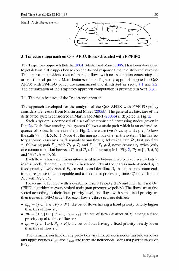
Fig. 2 A distributed system
3 Trajectory approach on QoS AFDX flows scheduled with FP/FIFO
The Trajectory approach (Martin 2004; Martin and Minet 2006a) has been developedto get deterministic upper bounds on end-to-end response time in distributed systems.This approach considers a set of sporadic flows with no assumption concerning thearrival time of packets. Main features of the Trajectory approach applied to QoSAFDX with FP/FIFO policy are summarized and illustrated in Sects. 3.1 and 3.2.The optimization of the Trajectory approach computation is presented in Sect. 3.3.
3.1 The main features of the Trajectory approach
The approach developed for the analysis of the QoS AFDX with FP/FIFO policyconsiders the results from Martin and Minet (2006b). The general architecture of thedistributed system considered in Martin and Minet (2006b) is depicted in Fig. 2.
Such a system is composed of a set of interconnected processing nodes (seven inFig. 2). Each flow crossing this system follows a static path which is an ordered se-quence of nodes. In the example in Fig. 2, there are two flows τ1 and τ2. τ1 followsthe path P1 = {4,5,6,7}. Node 4 is the ingress node of τ1 in the system. The Trajec-tory approach assumes, with regards to any flow τi following path Pi , that any flowτj following path Pj , with Pj �= Pi and Pj ∩ Pi �= ∅, never crosses τi twice (onlyone common portion between Pi and Pj ). In the example in Fig. 2, P2 = {1,5,6,3}and P1 ∩ P2 = {5,6}.
Each flow τi has a minimum inter-arrival time between two consecutive packets atingress node, denoted Ti , a maximum release jitter at the ingress node denoted Ji , afixed priority level denoted Pi , an end-to-end deadline Di that is the maximum end-to-end response time acceptable and a maximum processing time Ch
i on each nodeNh, with Nh ∈ Pi .
Flows are scheduled with a combined Fixed Priority (FP) and First In, First Out(FIFO) algorithm in every visited node (non preemptive policy). The flows are at firstsorted according to their fixed priority level, and flows with same fixed priority arethen treated in FIFO order. For each flow τi , three sets are defined:
• hpi = {j ∈ [1, n],Pj > Pi}, the set of flows having a fixed priority strictly higherthan this of flow τi ;
• spi = {j ∈ [1, n], j �= i,Pj = Pi}, the set of flows distinct of τi having a fixedpriority equal to this of flow τi ;
• lpi = {j ∈ [1, n],Pj < Pi}, the set of flows having a fixed priority strictly lowerthan this of flow τi ,
The transmission time of any packet on any link between nodes has known lowerand upper bounds Lmin and Lmax and there are neither collisions nor packet losses onlinks.

106 Real-Time Syst (2012) 48:101–133
The end-to-end response time of a packet is the sum of the times spent in eachcrossed node and the transmission delays on links. The transmission delays on linksare upper bounded by Lmax. The time spent by a packet m in a node Nh depends onthe static and dynamic higher priority packets in node Nh and on the delay due tothe non preemption of at most one lower priority packet. The higher priority packetscan be grouped into two categories. The first one contains the packets with the samefixed priority than packet m that have arrived in Nh before the arrival time of m in Nh
(all these packets have a higher dynamic priority than m, considering the FP/FIFOscheduling, and thus, will be processed before m). The other category includes thepackets with a higher fixed priority than packet m that have arrived before m beginsto be transmitted by Nh. The problem is then to upper bound the overall time spentin the visited nodes.
The solution proposed by the Trajectory approach is based on the busy periodconcept. A busy period of level L, as defined in Martin and Minet (2006b), is aninterval [t, t ′) such that t and t ′ are both idle times of level L and there is no idle timeof level L in (t, t ′). An idle time t of level L is a time such as all packets with prioritygreater than or equal to L generated before t have been processed at time t .
The Trajectory approach considers a packet m from flow τi generated at time t .It identifies the busy period and the packets impacting its end-to-end delay on all thenodes visited by m (starting from the last visited node backward to the ingress node).This decomposition enables the computation of the latest starting time of m on itslast node. This starting time can be computed recursively and leads to the worst caseend-to-end response time of the flow τi . This computation will be illustrated in thecontext of QoS AFDX.
The elements of the system considered in the Trajectory approach are instantiatedin the following way in the context of AFDX:
– each node of the system corresponds to an AFDX switch output port, including theoutput link,
– each link of the system corresponds to the switching fabric,– each flow corresponds to a VL path.
The assumptions of the Trajectory approach are verified by the existing AFDX (FIFOpolicy) and its evolution considered in this paper for QoS AFDX (FP/FIFO servicediscipline at switch output port level):
– the switching fabric delay is upper bounded by a constant value (16 µs) and mea-surements on AFDX switches show that this delay does not vary significantly, thus
L = Lmin = Lmax = 16 µs
– there are neither collisions nor packet loss on AFDX networks,– the routing of the VLs is statically defined,– VL parameters match the definition of sporadic flows in the following manner:
Ti = BAG, Chi = smax/R, Ji = 0
Since all the AFDX ports work at the same rate R = 100 Mb/s,
Chi = Ci = smax/R
for every node h in the network.

Real-Time Syst (2012) 48:101–133 107
Fig. 3 Illustrative AFDXconfiguration
Table 1 Illustrative AFDXconfiguration VL Priority BAG (µs) smax (bits) C (µs)
v1 1 4000 4000 40
v2 2 4000 4000 40
v3 2 4000 4000 40
v4 2 4000 4000 40
v5 2 4000 4000 40
3.2 Illustration on a sample AFDX configuration
Let us consider the sample AFDX configuration depicted in Fig. 3. The characteristicsof the five VLs v1, . . . , v5 which are transmitted on this AFDX network are givenin Table 1. v1 has the highest priority (1) and the four other VLs have the lowestpriority (2). Every link works at 100 Mb/s and the switching delay is 16 µs. Thetransmission time of a packet of 4000 bits on a link is 40 µs.
The FP/FIFO case is different from the purely FIFO case. Indeed, in a node, agiven packet m can be delayed by a higher priority packet which has arrived afterm in the node, or by a lower priority packet which is being transmitted at the arrivaltime of m in the node. It has an impact on the worst-case delay of m. Paragraph 3.2.1(resp. 3.2.2) shows how the Trajectory approach identifies the worst-case scenariofor a lowest priority packet (resp. a higher priority packet). Paragraph 3.2.3 exhibitsone source of pessimism of the Trajectory approach in the context of an AFDX net-work. This source of pessimism is similar for both the FP/FIFO and the purely FIFOcases. However, we will see in Sect. 3.3 that the limitation of this pessimism is morecomplex in the FP/FIFO case.
3.2.1 Identification of the worst-case for a packet with the lowest priority
Let us consider that VL v3 in Fig. 3 is under study. The worst-case delay for a packet3 of v3 occurs with a scheduling of packets leading to the latest starting time of 3 inits last node S3.
Figure 4 shows an arbitrary scheduling of the packets along the trajectory of v3.The packets are identified by their VL numbers (e.g. packet 3 is a packet from VL v3).The arrival time of a packet m in a node Nh is denoted a
Nhm . Time origin is arbitrarily
chosen as the arrival time of packet 3 in its source node e3. In each node, the packetsare processed with respect to the FP/FIFO policy. Consequently, packet 3 is delayedby packet 4 in S2. In node S3, packet 5 is delayed by packet 1 and delays packet 4,which delays packet 3.

108 Real-Time Syst (2012) 48:101–133
Fig. 4 An arbitrary scheduling of packets
Packet 3 from VL v3 crosses three busy periods
bpe3, bpS2, bpS3
on its trajectory, corresponding to the three nodes
N1 = e3, N2 = S2, N3 = S3
Let f (Ni) be the first packet which is processed in the busy period bpNi during whichpacket 3 is processed. Considering the scheduling in Fig. 4, we have
f (e3) = 3, f (S2) = 4, f (S3) = 1
As flows do not necessarily follow the same trajectory in the network, it is possiblethat packet f (Ni) does not come from the same previous node Ni−1 as packet 3.This case occurs in node S2, where packet 4 comes from node e4. It also occurs innode S3, where packet 1 comes from node S1. Therefore, p(Ni−1) is defined as thefirst packet which is processed in bpNi and comes from node Ni−1. Considering thescheduling in Fig. 4, we have
p(e3) = 3, p(S2) = 4
The starting time of packet 3 in node S3 is obtained by adding parts of the three busyperiods bpe3, bpS2, and bpS3 to the delays between the nodes, i.e. 2 × 16 µs. FromMartin and Minet (2006b), the part of the busy period bpNi which has to be addedis the processing time of packets between f (Ni) and p(Ni) minus the time elapsedbetween the arrivals of f (Ni) and p(Ni−1), i.e.
aNi
p(Ni−1)− a
Ni
f (Ni)
On the example in Fig. 4, the parts which have to be considered are:
– the transmission of packet 3 in node e3, i.e. 40 µs,– the time elapsed between the arrival of packet 3 and the end of processing of packet
4 in node S2, i.e. 4 µs,

Real-Time Syst (2012) 48:101–133 109
Fig. 5 Latest starting time of packet 3
– the time elapsed between the arrival of packet 4 and the end of processing of packet5 in node S3, i.e. 49 µs.
These parts are shown by thick lines on top of the packets in Fig. 4. Thus, the startingtime of packet 3 in node S3 on the example in Fig. 4 is:
40 + 4 + 49 + (2 × 16) = 125 µs
It has been shown (Martin and Minet 2006b) that the latest starting time of a packetm in its last node is reached when
(aNi
p(Ni−1)− a
Ni
f (Ni)) = 0
for every node Ni on the path of m. It comes to postpone the arrival time of everypacket joining the path of m in the node Ni in order to maximize the waiting time ofm in Ni .
The result of this postponing on the example in Fig. 4 is illustrated in Fig. 5. Thearrival time of packet 4 at node S2 is postponed to the arrival time of packet 3 at nodeS2. In node S3, packet 5 is postponed in order to arrive between packets 4 and 3, andpacket 1 is postponed in order to arrive not earlier than aS3
3 , packet 3 arrival time onnode S3 and before packet 3 departs from node S3.
Then, the worst case end-to-end delay of a packet is obtained by adding its lateststarting time on its last visited node and its processing time in this last node. Forpacket 3 in Fig. 5, this worst case end-to-end delay is
232 + 40 = 272 µs
More precisely, this delay includes the transmission times of packet 3 on node e3,packet 4 on node S2 and packets 4, 1, 5 and 3 on node S3. On this example, it can beseen that packets 3 and 4 are counted twice. Actually, it has been shown (Martin andMinet 2006b) that exactly one packet has to be counted twice in each node, exceptthe slowest one. In the context of the AFDX, all the nodes work at the same speed.Thus, the slowest node can be arbitrarily chosen as the last one. In the example inFig. 5, packet 3 and 4 are respectively counted twice in nodes e3 and S2. Packet 3is the longest one transmitted in nodes e3 and S2, while packet 4 is the longest onetransmitted in node S2 and S3.

110 Real-Time Syst (2012) 48:101–133
Fig. 6 Latest starting time of packet 1
3.2.2 Identification of the worst-case for a packet with a higher priority
The identification of a worst-case scenario for a packet with a higher priority is quitesimilar to what has been described in the previous section. The only difference con-cerns the non-preemption effect. Indeed, when a packet arrives in an output port, ithas to wait until the end of the packet under transmission in this port, regardless of thepriority of this packet. It means that even a packet with the highest possible prioritycan be delayed in an output port. The integration of this non-preemption effect in theTrajectory approach is now illustrated by studying the end-to-end delay of a packetfrom VL v1 on the AFDX configuration in Fig. 3. A worst-case scenario for v1 isdepicted in Fig. 6. In switch S1, packet 1 has the highest priority. Thus it cannot bedelayed by more than one lower priority packet. This packet has started transmissionan arbitrarily small instant ε before aS1
1 and it cannot be interrupted, due to the non-preemptive characteristic of AFDX. Here, this lower priority packet is packet 2 fromVL v2. The same scenario happens in switch S3, where v1 is the highest priorityflow, but is delayed by one packet of VL v5. Thus, the worst case end to end delay ofv1 is:
3 × C1 + C2 + C5 − 2 × ε + 2 × L = 5 × 40 − 2 × ε + 2 × 16
= 232 µs
3.2.3 Non optimality in the context of AFDX
Let us consider that a packet m is under study and a node Ni belongs to the trajectoryof m. The busy period of Ni in which m is transmitted includes packets coming fromthe same previous node as m and packets joining m in Ni . As it has been explainedin Paragraph 3.2.2, the worst-case scenario is built by the Trajectory approach in thefollowing way: the arrival time of every packet joining the trajectory of m in Ni ispostponed in order to maximize the waiting time of m in Ni . It means that the start ofthe busy period in Ni corresponds to the arrival time of the first packet coming fromthe same previous node as m. Consequently, a packet joining m in Ni cannot arrivebefore the first packet coming from the same previous node as m. Hence:
(a
Ni
p(Ni−1)− a
Ni
f (Ni)
) = 0

Real-Time Syst (2012) 48:101–133 111
Fig. 7 Latest starting time of VL v5
In the context of an AFDX network, for some VLs, it is not possible to find a schedul-ing which verifies this property for all the nodes of their trajectory.
Let us consider VL v5 of the example depicted in Fig. 3. bpS3 is the busy periodof level corresponding to the priority of packet 5. In order to maximize the delay ofpacket 5 in bpS3, the arrival time of packets 3 and 4 in S3 have to be as large aspossible, but not larger than the arrival time of packet 5 in node S3, because of theFIFO scheduling policy of flows with the same fixed priority:
aS33 ≤ aS3
5 and aS34 ≤ aS3
5 (1)
Since the two packets come from the same link, they are already serialized:∣∣∣aS3
3 − aS34
∣∣∣ ≥ C = 40 µs (2)
Without loss of generality, let us consider that packet 3 arrives before packet 4. From(1), we have:
aS34 = aS3
5 (3)
From (2) and (3), we have:
aS33 = aS3
5 − 40 µs (4)
The resulting worst-case scheduling is depicted in Fig. 7. p(e5) is packet 5 and f (S3)
is packet 3. From (4), we have (aS3p(e5) − aS3
f (S3)) ≥ 40 µs for any possible scheduling.
Thus, considering that (aNi
p(Ni−1)− a
Ni
f (Ni)) = 0 for every node Ni is a pessimistic
assumption in the context of the AFDX.
3.3 Optimization of the Trajectory approach computation
The optimization of the Trajectory approach computation aims at removing, or atleast limiting the pessimism induced by considering that the worst-case scenario for a

112 Real-Time Syst (2012) 48:101–133
packet m is obtained when (aNi
p(Ni−1)−a
Ni
f (Ni)) = 0 for every node Ni on the trajectory
of m. The idea is to compute a sure lower bound on the value of (aNi
p(Ni−1)− a
Ni
f (Ni))
for every node Ni on the trajectory of m. Such an optimization has been proposed inthe context of a purely FIFO AFDX (Bauer et al. 2010a). In the context of a FP/FIFOAFDX, the problem is slightly more complex, since packets with different fixed pri-orities have to be taken into account.
Paragraph 3.3.1 summarizes the basic computation of the FP/FIFO Trajectory ap-proach. Then, Paragraph 3.3.2 establishes a sure lower bound of (a
Ni
p(Ni−1)− a
Ni
f (Ni))
for every node Ni on the trajectory of m.
3.3.1 Basic computation
The computation of the worst-case end-to-end delay of a packet of a flow τi has beenformalized in Martin and Minet (2006b). In the context of this paper, all the nodeswork at the same rate and the jitter in each emitting node is null. Thus, the worst caseend-to-end response time of any flow τi is bounded by:
Ri = maxt≥0
(W
lastii,t + Ci − t
)
lasti is the last visited node of flow τi and Wlastii,t is a bound on the latest starting time
of a packet m generated at time t on its last visited node. The definition of Wlastii,t
given in Martin and Minet (2006b) becomes:
Wlastii,t =
∑
j∈spi∪{i}]Pj ∩Pi �=∅
(1 +
⌊t + Ai,j
Tj
⌋)· Cj (5)
+∑
j∈hpiPj ∩Pi �=∅
⎛
⎝1 +⎢⎢⎢⎣
Wlasti,ji,t + Bi,j
Tj
⎥⎥⎥⎦
⎞
⎠ · Cj (6)
+∑
h∈Pih�=lasti
⎛
⎜⎝ max
j∈hpi∪spi∪{i}h∈Pj
{Cj
}⎞
⎟⎠ (7)
+ (|Pi | − 1) · Lmax (8)
+∑
Nh∈Pi
δhi (9)
−∑
Nh∈PiNh �=firsti
ΔNh(10)
− Ci (11)

Real-Time Syst (2012) 48:101–133 113
Where
ΔNh= a
Nh
p(Nh−1)− a
Nh
f (Nh) (12)
The meaning of the different terms which compose Wlastii,t is the following.
– Term (5) corresponds to the processing time of packets from flows, crossing theflow τi , with a fixed priority level equal to this of τi and transmitted in the samebusy period as m. Ai,j integrates, for flows τi and τj , the maximum difference onthe delay between their source node and their first shared output port.
– Term (6) is similar to the previous one, but concerns the packets from flows witha fixed priority level higher than this of τi . Bi,j integrates, for flows τi and τj ,the maximum difference on the delay between their source node and their lastshared output port. Indeed, higher priority packet can overtake m until its effective
transmission in their last shared node (Wlasti,ji,t ). The amount of packet that can
delay the departure of packet m in its last node has thus to be computed iteratively.– Term (7) is the processing time of the longest packet for each node of path Pi ,
except the last one. It represents the packets which have to be counted twice, asexplained in Paragraph 3.2.1.
– Term (8) corresponds to the sum of switching delay.– Term (9) corresponds to the maximum delay due to the non preemption of packets
with a fixed priority lower than this of τi . In each node h, it is the transmissiontime of the biggest lower priority packet of a flow τj crossing flow τi in this node.It is denoted δh
i .– Term (10) sums for each node Nh in Pi the duration between the beginning of the
busy period and the arrival of the first packet coming from the preceding node inPi , i.e. Nh−1. This term is null in the context of Martin and Minet (2006b).
– Ci is subtracted, because Wlastii,t is the latest starting time and not the ending time
of the packet from τi on its last node.
The differences between the FIFO and the FP/FIFO computations are Terms (6)and (9), which take into account the packets with a higher or a lower fixed prior-ity level. These terms are obviously null in the FIFO context.
Solving
Ri = maxt≥0
(W
lastii,t + Ci − t
)
comes to find the maximum vertical deviation between the function
t → Wlastii,t + Ci
and the identity function
t → t
This computation is illustrated on VL v3 in Fig. 3. As there is no flow with a fixedpriority lower than this of v3, the term (9) is null. For this basic computation, Term

114 Real-Time Syst (2012) 48:101–133
Fig. 8 Input and output ports ofa switch
(10) is also null:
WS33,t + C3 =
(
1 +⌊
WS33,t + B3,1
T1
⌋)
· C1 +(
1 +⌊
t + A3,4
T4
⌋)· C4
+(
1 +⌊
t + A3,5
T5
⌋)· C5 +
(1 +
⌊t
T3 + A3,3
⌋)· C3
+ maxj with e3∈Pj
{Cj
} + maxj with S2∈Pj
{Cj
} − C3
+ (|P3| − 1) · Lmax + C3
=(
1 +⌊
WS33,t + 40
4000
⌋)
· 40 +(
1 +⌊
t + 40
4000
⌋)· 40
+(
1 +⌊
t + 40
4000
⌋)· 40 +
(1 +
⌊t
4000
⌋)· 40
+ 40 + 40 − 40 + (3 − 1) × 16 + 40
= 272 + 120
⌊t + 40
4000
⌋+ 40
⌊WS3
3,t + 40
4000
⌋
The upper-bound on the end-to-end delay is reached for t = 0 and RS35 = 272 µs.
3.3.2 Optimization of the computation in the context of the AFDX
The optimization of this computation in the context of the AFDX concerns Term(10). Indeed, it has been shown in Paragraph 3.2.3 that, for some VLs, there exists noscheduling leading to
ΔNh= a
Nh
p(Nh−1)− a
Nh
f (Nh) = 0, ∀Nh ∈ Pi
In the following, we establish a lower bound on ΔNh∀Nh ∈ Pi and we prove its
correctness. This result is an extension of the one proven in Bauer et al. (2010a).Let us consider the part of a switch depicted in Fig. 8. It includes kh + 1 input
ports and one output port. Each input port IPhi receives a sequence of packets seqh
i
which are all transmitted on the output port OPh.This part of a switch corresponds to a node in the Trajectory approach.

Real-Time Syst (2012) 48:101–133 115
Fig. 9 Illustration of ΔNh
The two next paragraphs address the optimization of the computation in the FIFOcontext (addressed in Bauer et al. 2010a) and its generalization in the FP/FIFO con-text (not addressed in Bauer et al. 2010a).
The FIFO context The value of ΔNhin this node in a FIFO context (one single
priority level) is illustrated in Fig. 9. A sure lower bound for ΔNhin this context has
been given in Bauer et al. (2010a).The packet m of flow τi under study is sent on the output link OPh in a busy period
bpNh . The packets which compose bpNh in the worst case scenario are determinedthanks to terms (5), (6) and (9). These packets are grouped by input link. IPh
0 is theinput link of τi , while IPh
x (1 ≤ x ≤ kh) are the other input links. Sequence seqhx
(0 ≤ x ≤ kh) contains the packets of bpNh coming form IPhx .
As defined in (12), ΔNhis the delay between the earliest arrival of a packet of
bpNh (i.e. the beginning of bpNh ) and the arrival of the first packet of bpNh comingfrom IPh
0 . In Fig. 9, ΔNhis the difference between the arrival of p3 and the arrival of
p(Nh−1).In order to maximize the delay of packet m in node Nh, sequences of packets
having a fixed priority equal to this of m are postponed so that the last packet ofeach sequence arrives at the same time θ as packet m. Indeed, these packets cannotdelay packet m if they arrive after time θ . This construction is a generalization of theTrajectory approach presented in Martin and Minet (2006b): instead of postponingindividually each packet, we only postpone sequences of already serialized packets.
The latest starting time of m in its last node is maximized when∑
Nh∈PiNh �=firsti
(ΔNh)
is minimized. It comes to determine the lower bound of each term ΔNhof the sum.

116 Real-Time Syst (2012) 48:101–133
From (12), it comes that the minimum value of ΔNhis obtained by minimizing
aNh
p(Nh−1)and maximizing a
Nh
f (Nh).
Let us define lhx (0 ≤ x ≤ kh) as the duration of sequence seqhx without its first
packet. Then, we have:
aNh
f (Nh) = θ − max1≤x≤kh
lhx (13)
aNh
p(Nh−1)= θ − lh0 (14)
Consequently, minimizing aNh
p(Nh−1)comes to maximize lh0 . It is obtained when the
smallest packet of sequence seqh0 is transmitted at the beginning of seqh
0 .
Similarly, maximizing aNh
f (Nh) comes to minimize each lhx for 1 ≤ x ≤ kh. It is
obtained when the largest packet of sequence seqhx is transmitted at the beginning of
seqhx , for 1 ≤ x ≤ kh.To summarize, in the FIFO context, ΔNh
is lower bounded by the maximum of 0and:
max1≤x≤kh
(min
(lhx
))− max
(lh0
)− max
y∈lpih−1∈Py
Chy (15)
The FP/FIFO context In the context of an FP/FIFO policy, there are packets withlower and higher priorities than m. These two types of packets have to be consideredin the computation of a sure lower bound for ΔNh
.Let us consider first the case of the lower priority packets. Their only impact is
due to the non preemption effect. It means that one single lower priority packet candelay m, provided it is under transmission at the arrival instant of f (Nh). In orderto maximize this effect, this lower priority packet has to be as long as possible andit has to start transmission immediately before the arrival of f (Nh). This worst-caseis depicted in Fig. 10, where this lower priority packet arrives from IPh
0 . The effectof this lower priority packet is to shorten ΔNh
. Indeed, it is equivalent to say thatno packet with the same priority as m arrives before the end of transmission of thislongest lower priority packet. Therefore, the transmission time of this longest lowerpriority packet is subtracted from ΔNh
.Second, we consider packets with a higher fixed priority (τj ∈ hpi ). These packets
can delay packet m even if they arrive on node h after time θ . In order to find thesmallest possible value of ΔNh
, the sequence seqh0 has to be as long as possible, while
the sequences seqhx (1 ≤ x ≤ kh) have to be as short as possible. This is achieved by
placing all higher priority packets coming from IPh0 in seqh
0 (i.e. before θ ) and allhigher priority packets coming from IPh
x (1 ≤ x ≤ kh) after θ . This is depicted inFig. 11. Then, transmission times of higher priority packets coming from IPh
0 aresubtracted from ΔNh
and the other higher priority packets have no effect on ΔNh.
3.4 Results on the sample AFDX configuration
The end-to-end delay upper bounds for all the VLs of the configuration in Fig. 3 arepresented in Table 2. The BT row corresponds to the classical Trajectory approach

Real-Time Syst (2012) 48:101–133 117
Fig. 10 Impact of lower priority packets on ΔNh
Table 2 Obtained end-to-enddelay upper bounds in µs
EWC: exact worst-caseBT: basic Trajectory approachOT: optimized Trajectoryapproach
VL EWC (µs) BT (µs) OT (µs)
v1 232 232 232
v2 192 192 192
v3 272 272 272
v4 272 272 272
v5 176 216 176
for FP/FIFO scheduled flows. The OT row gives the enhanced results obtained by ap-plying the grouping optimization. The exact worst case, that can be obtained on thissmall example with a model checking tool, is also presented in Table 2 for compar-ison purpose. The network calculus approach is not considered since it has not beenapplied to the AFDX for FP/FIFO scheduled flows.
There are four VLs (v1, v2, v3 and v4) for which the basic Trajectory approachgives the exact worst case. However, for VL v5, the basic Trajectory approach intro-duces a 40 µs pessimism, which is eliminated by the optimization of the computation.
4 Evaluation of the pessimism of the obtained upper bounds
It has been shown in Bauer et al. (2010a) that, in the context of an AFDX with FIFOpolicy, the upper bounds computed by an optimized Trajectory approach are stillpessimistic. This pessimism has been bounded and it appears that, on realistic AFDX

118 Real-Time Syst (2012) 48:101–133
Fig. 11 Impact of all higher packets on ΔNh
configurations, the upper bounds computed by the Trajectory approach are on averageat least two times less pessimistic than the upper bounds computed by the NetworkCalculus approach (Bauer et al. 2010a). In this section, an extension of the processused for the evaluation of the pessimism in the context of an AFDX with FIFO policyis proposed. This extended process can cope with an AFDX with FP/FIFO policy.Thus, it integrates packets with a fixed priority level which is not the same as the oneof the packet under study. The goal is to compare the pessimism of the Trajectoryapproach applied to an AFDX with FP/FIFO policy to the pessimism of both theNetwork Calculus and the Trajectory approaches applied to an AFDX with FIFOpolicy.
For a given path of a given VL, the pessimism of the upper bound computed by theTrajectory approach is the difference between the exact worst-case end-to-end delayof a frame transmitted on this path and the computed upper bound. For complexAFDX networks, the exact worst-case end-to-end delay is unknown. Then, the ideais to compute a sure upper bound of this difference. The principle has been introducedin Bauer et al. (2010b) for an AFDX with a FIFO policy. It is illustrated in Fig. 12.A sure lower bound of the worst-case end-to-end delay is computed. It is obtained bygenerating a scenario which is as close as possible from the exact worst-case scenario.It is called the unfavorable scenario in Fig. 12. Then, the difference between this surelower bound and the sure upper bound computed by the Trajectory approach gives anupper bound on the pessimism of the Trajectory approach.
Principle of the generation of an unfavorable scenario The key point of this pro-cess is the generation of the unfavorable scenario. A scenario is unfavorable for a

Real-Time Syst (2012) 48:101–133 119
Fig. 12 Evaluation of the pessimism of the Trajectory approach
given path of a given VL if the packet of this flow is delayed as much as possiblein each output port that the packet crosses. The generation of this unfavorable sce-nario is done by associating offsets to all the VLs which cross the VL vi under study.The offsets are assigned so that the sequences of packets in each input link of eachnode are synchronized in the same way as in Fig. 11. The generation proceeds in thefollowing steps.
First, the packets contained in the sequence of each input link are determined. Inorder to do that, it is assumed that vi and all the VLs which cross vi emit exactlyone packet. All the other VLs of the configuration emit no packet. This assumptionis valid, since VLs are defined as sporadic flows. Under this assumption, the packetscontained in the sequence of each input link are known. IPh
0 is defined as the inputport of vi in the node h.
Second, the instants of reception of the packets joining vi (i.e. coming from aninput link which is not IPh
0), are determined using the following criteria:
– the packets with the same priority as vi are placed in separate queues, depending ontheir incoming port. The packets are ordered in the queues by decreasing transmis-sion time (i.e. decreasing packet size), in order to avoid holes in further sequencesof reception, as exemplified in Bauer et al. (2010a),
– higher priority packets are all placed in a unique queue and are sorted by decreasingsize,
– the longest lower priority packet is selected for each input link.
Based on this criteria, the instant of reception of the packets are decided as follows.
– First the packets with the same priority as vi are considered. All the queues in-cluding these packets are aligned with the sequence coming from IPh
0 in order tohave the same arrival time for the last packet of each sequence. It corresponds tothe process which has been described in Bauer et al. (2010a) for the FIFO case.By this way, all the packets with the same priority as vi delay m, since they arriveat the output port no later than m. Moreover, they arrive at the output port as lateas possible, in order to maximize their effect on m. The arriving time of the lastpacket of each sequence is called θ .

120 Real-Time Syst (2012) 48:101–133
– Second, the impact of the non preemption effect of each of the selected lowerpriority packets is considered. Each selected packet is placed in order to delay asmuch as possible the starting time of the first packet of the longest sequence. Onlythe lower priority packet which has the biggest impact on the delay of the packetswith the same priority as vi is kept. The amount of packets with the same priorityas m, plus the impact of one lower priority packet, leads to a possible transmissiontime θ0 for packet m.
– Third, the higher priority packets are considered. These packets can be served be-fore m even if they arrive after θ . Moreover, since the higher priority packets aresorted by decreasing size, the whole burst can be served before m, if the first packetis served before m. The idea is then to place the first higher priority packet so thatit is received no later than θ0. If the transmission time of this longest higher prior-ity packet is less than (θ0 − θ ), this can be achieved by positioning the beginningof the sequence of higher priority packets at θ . Otherwise, this sequence has to beshifted before θ . Consequently, the sequence of packets with the same priority asvi coming from the same input link as the longest highest priority packet is broughtforward.
Finally, the packets are placed in the output buffer according to the FP/FIFO policy:the first available packet with the highest priority is served first. When two or morepackets with the same priority become available at the same time, the packets comingfrom an input link other than IPh
0 are served first. Thus m is always the last servedpacket.
Example of the generation of an unfavorable scenario The generation of the unfa-vorable scenarios is illustrated on the small example that has been presented in Fig. 3.The flow v1 from e1 has a higher priority than all other flows. Thus, it is only im-pacted by the non preemption effect of packets of lower priority. This happens innodes S1 and S3 (see Fig. 13). In node S1, packet 2 is placed just before the arrivaltime of packet 1, hence it is served first. Packet 2 does not follow packet 1 in thenext node. Thus, packet 1 is alone in IPS3
S1. The non preemption effect due to packet
3, 4 or 5 in node S3 is the same. Any of them can be placed just before packet 1.Let us suppose that it is packet 4. Then, it is served before packet 1. The resultingend-to-end delay for packet 1 is three times its transmission time, plus two delays onlinks, plus the transmission time of packets 2 and 4 (minus ε, with ε > 0). This gives:
3 × 40 + 2 × 16 + 2 × (40 − ε) < 232 µs
The flow v3 follows a trajectory that is quite similar to the trajectory of v1. Theunfavorable scenario for v3 is depicted in Fig. 14. Packets 3 and 4 have the samepriority. Thus, they arrive in S2 at the same time and packet 4 if served first. In thefollowing node, the sequence in IPS3
S2 is the same as the sequence on the output portof S2. Packet 5 has the same priority level, thus, it is placed at the arrival time ofpacket 3. Packets 4 and 5 create a sufficient amount of backlog at the arrival time ofpacket 3 (in fact, the transmission time of packet 5) and it is possible to place packet1 just after the arrival of packet 3. It will still be served before packet 3 because ofits higher priority level. The resulting end-to-end delay for packet 3 is three times its

Real-Time Syst (2012) 48:101–133 121
Fig. 13 Unfavorable scenario for packet 1 leading to a high end-to-end delay
transmission time, plus two delays on links, plus the transmission time of packets 4,5 and 1. This gives:
3 × 40 + 2 × 16 + 3 × 40 = 272 µs
The generation of an unfavorable scenario for v2 is depicted in Fig. 15. This caseillustrates the fact that a higher priority packet can not always be placed after theconsidered packet. Here in node S1, packet 2 is alone in its queue. In order to beprocessed before packet 2, packet 1 has to arrive at least at the same time as packet 2.Again, packet 2 is alone in the last node. The resulting end-to-end delay for packet 2is three times its transmission time, plus two delays on links, plus the transmissiontime of packet 1 in node S1. This gives:
3 × 40 + 2 × 16 + 40 = 192 µs
The serialization of packets is of course taken into account by the process. This isillustrated with the scenario generated for v5 in Fig. 16. In node S3, packet 5 meetsone higher priority packet (1) coming from node S1 and two packets (3 and 4) ofsame priority coming from node S2. Packets 3 and 4 are in a sequence of their own,thus they are serialized. This sequence is shifted so that the last packet (here packet 3)

122 Real-Time Syst (2012) 48:101–133
Fig. 14 Unfavorable scenario for packet 3 leading to a high end-to-end delay
arrives at the arrival time of packet 5. Hence, packet 4 is served too early and cannotdelay packet 5. There is though enough backlog in order to place packet 1 after thelower priority packets. The resulting end-to-end delay for packet 5 is two times itstransmission time, plus one delay on the link between e5 and S3, plus the transmissiontime of packets 3 and 5 in node S3. This gives:
2 × 40 + 16 + 2 × 40 = 176 µs
All the delays computed on this sample configuration are summarized in Table 3.We compare the delay of the unfavorable scenario with the upper bound obtained withthe optimized Trajectory approach. On this example, the generated scenario matcheswith the worst case for each flow.
5 Case study: a representative part of an industrial AFDX network
In this case study, the optimized Trajectory approach is applied on a real AFDXconfiguration to which non avionics flows have been added. The goal is to evaluateto which extent the well-known properties of the FP/FIFO policy are kept by theobtained upper bounds of the end-to-end delays. Two levels of priority are used. The

Real-Time Syst (2012) 48:101–133 123
Fig. 15 Unfavorable scenario for packet 2 leading to a high end-to-end delay
Fig. 16 Unfavorable scenario for packet 5 leading to a high end-to-end delay
higher one is allocated to the avionics flows, while the lower one is allocated to nonavionics flows. The case study gives some results about:
– the impact of the non avionics flows on the upper bounds of the end-to-end delaysof the avionics flows,
– the pessimism of the upper bounds computed for the non avionics flows.

124 Real-Time Syst (2012) 48:101–133
Table 3 Unfavorable scenariocompared to the computed upperbounds
EWC: exact worst-caseBT: basic Trajectory approachOT: optimized TrajectoryapproachHeur: unfavorable scenario
VL EWC (µs) BT (µs) OT (µs) Heur (µs)
v1 232 232 232 232
v2 192 192 192 192
v3 272 272 272 272
v4 272 272 272 272
v5 176 216 176 176
Fig. 17 An AFDX configuration with additional lower priority flows
Paragraph 5.1 briefly describes the AFDX configuration which is used for the casestudy. Paragraph 5.2 gives the upper bounds obtained by the optimized Trajectoryapproach, considering both FIFO and FP/FIFO policies. Paragraph 5.3 gives the im-provement brought by the optimization of the Trajectory approach in the context ofthe FP/FIFO policy. Finally, Paragraph 5.4 evaluates the pessimism of the obtainedupper bounds, thanks to the process presented in Sect. 4.
5.1 An AFDX network with additional lower priority flows
The results presented in this section are based on the AFDX architecture depicted inFig. 17. This configuration is a representative part of an industrial AFDX network.The part considered in this study includes 21 end systems, four switches and 91 VLs.Each avionics system is distributed on different end systems connected through VLs.The reference VL for this case study is the avionics one connecting end system ES0

Real-Time Syst (2012) 48:101–133 125
to end system ESDEST. It crosses switches SW1 and SW2. This flow is denoted VL0.It has the following parameters: BAG = 32 ms and smax = 384 bytes.
In this configuration, 18 end systems are added to the reference network. Each ofthem emits one non avionics (lower priority) flow. These VLs increase the load onthe output ports of the AFDX switches. In Fig. 17, thin arrows designate VLs whichshare only the output port of SW1 with VL0, while bold arrows designate VLs whichalso share the output port of SW2 with VL0. These additional VLs all have the samesmax and BAG parameters. The values of these parameters correspond to a given loadin the output ports of the switches.
All the worst case end-to-end delay results presented in this section have beencomputed with a dedicated tool developed in Python which implements the optimizedTrajectory approach with both FIFO and FP/FIFO policies. The worst case end-to-end delay of VL0 is 2397 µs when there are no non avionics flows. This value is areference for the evaluation of the impact of the additional load on the avionics traffic.The obtained upper bounds for the non avionics traffic are given for one non avionicsVL. This VL is generated by ESLoad 1-1 and shares both output ports of SW1 andSW2 with VL0. We take the output port of switch SW1 as a reference for the loadinformation. As all the additional VLs have identical parameters, the variation of loadin switch SW1 is representative of the global network load variation. The initial loadin the output port of switch SW1 without any additional load is about 13%.
5.2 Impact of a fixed priority strategy
As previously mentioned, adding lower priority traffic to the existing avionics trafficis a promising idea in order to better use available network resource. However, thisefficiency improvement should in no case impact the determinism of avionics dataflows. The determinism of those flows is closely related to their worst case end-to-enddelays. Thus, the upper bounds of these end-to-end delays have been computed forthe reference VL0 for different additional loads traffic. The first results concern theevolution of response time with a FIFO algorithm. This gives a reference to measurethe gain obtained thanks to a FP/FIFO scheduling strategy. The results for FIFO aredepicted in Fig. 18. Both end-to-end delay analysis are conducted with our tool whichfeatures the Trajectory approach optimization presented in Sect. 3.3.
Each flow generates a load depending on its BAG and smax parameters. A givenload can correspond to many (BAG, smax) combinations. If we do not consider theper-frame overhead, the same information can be sent with 80 bytes frames every8 ms, with 160 bytes frames every 16 ms or with 320 bytes frames every 32 ms,and so on. . . In AFDX networks, the BAG values are harmonic periods between 1 msand 128 ms. smax is limited by the standard Ethernet frame size. In Fig. 18, curvesrepresent iso-load evolutions. The reference line is the end-to-end response time withno additional load. Each point corresponds to a (BAG, smax) couple. The BAG valueis given on the horizontal axis and the smax value is displayed next to the point.
In the FIFO case, the end-to-end delay of VL0 is mainly impacted by the smax ofthe additional flows even at low level loads: the impact of a 37% additional load with(BAG = 1 ms, smax = 384 B) parameters is lower than for a 1% load and (64 ms,640 B) parameters. Generally, the impact goes lower with lower smax values. This is

126 Real-Time Syst (2012) 48:101–133
Fig. 18 Impact of an additional load on the end-to-end delay of VL0 with a FIFO policy
because in the worst case and for relatively low loads, an avionics packet will haveto wait in an output port during the transmission of packets from other flows, whichdirectly depends on their size. Moreover, using only minimal packet size generates ahigh amount of overhead.
The results confirm that FIFO cannot cope with such a traffic increase.
5.2.1 Bounding the impact on the existing avionics flows
Let us now consider that the flows are scheduled with a FP/FIFO policy. As previ-ously mentioned, avionics flows are allocated the higher priority, while non avionicsflows are allocated the lower priority. The results are depicted in Fig. 19. This fig-ure gives the same type of information on worst case end-to-end delays of VL0 thatFig. 18.
Not surprisingly, the results for VL0 with FP/FIFO are much better than withFIFO. Although there is still an impact on avionics worst case end-to-end responsetimes with increasing packet size, the increase is much more limited. The delay in-crease with 1024B packets is up to 20% lower than in FIFO. An avionics VL isstill delayed by lower priority level flows, but only due to the non preemption effect,which directly depends on the size of the lower priority packets.
The only packet of lower priority that can delay an avionics packet in a switchoutput port is a packet that is already being served. As the avionics load is constant,the end-to-end delay bound only depends on the smax parameter of the lower priorityflows. Indeed, it can be observed that all the point with a similar smax value are alignedand correspond to a given worst case end-to-end delay for VL0. This means thatthe impact on avionics traffic can easily be contained, simply by limiting the smax
parameter of the additional traffic, independently of the load. This requirement is

Real-Time Syst (2012) 48:101–133 127
Fig. 19 Impact of an additional load on the end-to-end delay of VL0 with a FP/FIFO policy
easy to specify and guarantees some scalability for future increase of the additionalload.
5.2.2 Impact of BAG and smax on lower priority flows
For the lower priority flows, FP/FIFO and FIFO results are quite similar: as thesesflows represent the major part of the traffic, the impact of the higher priority avionicsflows is discernible only for very low loads. The results for the FP/FIFO case arepresented in Fig. 20.
The worst case end-to-end delays decrease with the smax value for two reasons:
– since frames are shorter, their transmission time is shorter,– the other additional flows send shorter packets that create less congestion in the
output ports.
This decreasing is less significant for very small BAGs, because a lower prioritypacket can be delayed by more than one packet from another source.
5.3 Gain of the grouping optimization
In this paragraph, the gain brought by the optimization of the Trajectory approach isevaluated for both avionics and non avionics flows.
5.3.1 Gain for high priority VL0
The gain brought by the grouping optimization for the avionics flow VL0 is presentedin Table 4. The results are given for different additional lower priority traffic loads.

128 Real-Time Syst (2012) 48:101–133
Fig. 20 Impact of an additional load on the end-to-end delay of VLLoad1-1 with a FP/FIFO policy
Table 4 Gain of the grouping optimization on VL0 worst case end-to-end delay
BAG 0%load
1%load
3%load
6%load
18%load
37%load
45%load
1 ms
11.4%
– – 11.1% 10.7% 10.0% 9.6%
2 ms – 11.1% 10.9% 10.0% 8.7% 8.0%
4 ms – 10.9% 10.4% 8.7% 6.2% –
8 ms 11.1% 10.4% 9.5% – – –
16 ms 10.8% 9.5% 7.8% – – –
32 ms 10.2% 7.8% – – – –
64 ms 9.1% – – – – –
128 ms 7.0% – – – – –
The empty cells correspond to impossible combinations of BAG and smax values (be-cause of the AFDX frame minimal and maximal size). The 0% row corresponds tothe initial avionics configuration without additional traffic. In this case, the gain of thegrouping optimization is 11.4%. With additional load, the gain of the optimization isstill existing, but decreases when the load increases. Actually, we show in Fig. 21that the evolution of the gain is directly linked to the smax parameter of the additionalload. Indeed, in the ΔNh
computation, the only impact of lower priority flows is thetransmission time of one lower priority packet, due to the non preemption effect.
The worst case end-to-end delay without the grouping optimization for VL0 is2704 µs. With the optimization, this bound falls to 2397 µs. This represents the initial11.4% gain. With a 16% additional load of 1536 bytes packets and a 16 ms BAG, thebound without optimization raises up to 2950 µs. This raise corresponds to the 246 µs

Real-Time Syst (2012) 48:101–133 129
Fig. 21 Gain of the serialization optimization on VL0 worst case end-to-end delay
needed to transmit two 1536 bytes packets due to the non preemption effect. With theoptimization, the bound raises up to 2766 µs. This 369 µs raise corresponds to thetransmission time of three 1536 bytes packets (3 × 1536 × 8/100 = 368.64 µs). Twoof them correspond to the non preemption effect, as previously. The third packet isremoved from ΔNh
in the worst case end-to-end delay computation of VL0 in nodeSW-1. Indeed, this is the node where the grouping phenomenon occurs: VL0 meets30 already serialized avionics flows coming from switch SW-3. In the worst case, thetransmission time of a packet of lower priority has to be subtracted from ΔNh
. Thisis where the third occurrence of a 1536 bytes lower priority packet has to be counted.
5.3.2 Gain for lower priority VLLoad1-1
In Table 5, the gain of the optimization for each amount of additional traffic is sum-marized. The gain is higher for larger packet sizes (for each row, the packet size isproportional to the BAG). The delay introduced by the six lower priority serializedflows from switch SW-3 that cross the path of VLLoad1-1 in switch SW-1 is reducedto only one with the grouping optimization. The five packet gain is thus higher forlarger packet sizes. If we consider the configuration in the case of a 128 ms BAGand a 1280 bytes packet size (last row of the first column), the optimization gainis 631.76 µs. This corresponds to the transmission time of five 1280 bytes pack-ets (5 × 1280 × 8/100 = 512 µs) and the transmission time of one higher prioritypacket of 1497 bytes (119.76 µs). This packet is from VL567. Because of the smallBAG of this VL (2 ms), more than one packet from this flow can delay a packet fromVLLoad1-1. In fact, the serialization optimization reduces this phenomenon which hap-pens with high loads and low BAG values. This explains also the upturn in the twolast rows of Table 5 for the smallest BAG value.

130 Real-Time Syst (2012) 48:101–133
Table 5 Average gain of thegrouping optimization onVLLoad1-1 worst caseend-to-end delay
BAG 1%load
3%load
6%load
18%load
37%load
45%load
1 – – 5.0% 6.1% 15.4% 16.8%
2 – 5.1% 5.7% 7.9% 10.0% 10.8%
4 – 5.8% 7.1% 12.6% 20.2% –
8 5.3% 7.1% 9.3% 14.5% – –
16 6.2% 9.3% 12.3% – – –
32 7.7% 12.3% – – – –
64 10.3% – – – – –
128 13.5% – – – – –
Fig. 22 Trajectory end-to-end delay maximum pessimism with FP/FIFO
5.4 Pessimism of the obtained upper bounds
A sure lower bound of the end-to-end delay has been computed for all the paths ofthe avionics configuration evaluated in this paper, considering the unfavorable sce-narios. Based on these sure lower bounds, the pessimism of the Trajectory approachfor this configuration with FP/FIFO is summarized in Fig. 22. This is an averagemeasurement of all the possible (BAG, smax) combinations.
The maximum pessimism of the end-to-end delay bounds is always inferiorto 28%. For about 4% of the flows, the pessimism is null. This means that for thoseflows, the optimized trajectory approach computes the worst case end-to-end delay.The average bound on the pessimism considering all the flows is 8.7% with staticpriority scheduling. The average bound on the pessimism has been computed consid-

Real-Time Syst (2012) 48:101–133 131
ering the results obtained in a FIFO context (same priority for all the flows) by boththe optimized Trajectory approach and the Network Calculus one. The result is 6.2%for the Trajectory approach and 14% for the Network Calculus one. It means that, onthe configuration considered in this case study, the Trajectory approach with FP/FIFOis slightly more pessimistic than the same approach with FIFO and significantly lesspessimistic than the Network Calculus approach with FIFO.
6 Conclusion
In this paper, we first demonstrate that the Trajectory approach with FP/FIFOscheduling is able to guarantee worst case end-to-end delays for AFDX networkswith static priority flows differentiation QoS mechanisms.
Then we show how this approach can be enhanced in the AFDX context by takinginto account the serialization on links (grouping technique optimization). This im-provement allows to compute tighter upper-bounds on end-to-end delays. It has beenillustrated on a sample AFDX configuration.
Then, we analyze the impact of additional low priority traffic on a representativepart of an industrial AFDX network. We showed that the impact of low priority flowscan be upper bounded per switch by the transmission time of the biggest lower prior-ity packet (non preemption effect). Moreover, as the load induced by avionics flows islow, we conclude that the impact of FP/FIFO policy on lower priority flows is limited.
The pessimism of the Trajectory approach in the context of FP/FIFO is limited.On the case study considered in this paper, the average upper bound of this pes-simism is 8.7%. It means that the obtained upper bounds are quite close from theexact worst-case delays. Consequently, a further reduction of the upper bounds needsfurther assumptions.
One of these assumptions concerns a partial synchronization of the flows. Indeed,a subset of the VLs transmitted on an AFDX network are strictly periodic. When twoor more of these periodic VLs are emitted by the same end system, they are sched-uled and it is possible to determine minimum durations between frames of differentVLs. The integration of these minimum durations in the worst-case analysis can bevaluable, as it has been shown in Li et al. (2010). Further studies are needed in thisdirection.
Another extension of the work presented in this paper concerns the integrationof other scheduling policies, such as Weighted Fair Queueing (Parekh and Gallager1993). The idea is to dynamically share the remaining bandwidth between differentnon avionics flows.
References
ARINC-664 (2002–2005) ARINC specification 664: Aircraft data network, Parts 1, 2, 7. Tech rep,Aeronotical Radio Inc
Bauer H, Scharbarg JL, Fraboul C (2009) Applying and optimizing trajectory approach for performanceevaluation of AFDX avionics network. In: Proc of the 14th international conference on emergingtechnologies and factory automation, IEEE, Mallorca, Spain

132 Real-Time Syst (2012) 48:101–133
Bauer H, Scharbarg JL, Fraboul C (2010a) Improving the worst-case delay analysis of an AFDX networkusing an optimized trajectory approach. IEEE Trans Ind Inf 6(4):521–533
Bauer H, Scharbarg JL, Fraboul C (2010b) Worst-case end-to-end delay analysis of an avionics AFDXnetwork. In: Design automation and test in Europe conference and exhibition 2010, DATE’10, IEEE,Dresden, Germany
Charara H, Scharbarg JL, Ermont J, Fraboul C (2006) Methods for bounding end-to-end delays on anAFDX network. In: Proceedings of the 18th ECRTS, Dresden, Germany
Frances F, Fraboul C, Grieu J (2006) Using network calculus to optimize the AFDX network. In: Proceed-ings of ERTS, Toulouse, France
Grieu J (2004) Analyse et évaluation de techniques de commutation Ethernet pour l’interconnexion dessystèmes avioniques. PhD thesis, INP-ENSEEIHT, France
Itier JB (2007) A380 integrated modular avionics. In: Proceedings of the ARTIST2 meeting on integratedmodular avionics, vol 1(2), pp 72–75. http://www.artist-embedded.org/artist
Jasperneite J, Neumann P, Theis M, Watson K (2002) Deterministic real-time communication withswitched ethernet. In: Proceedings of the 4th IEEE international workshop on factory communicationsystems. IEEE Press, Västeras, pp 11–18
Li X, Scharbarg JL, Fraboul C (2010) Improving end-to-end delay upper bounds on an afdx network byintegrating offsets in worst-case analysis. In: Proc of the 14th international conference on emergingtechnologies and factory automation, Bilbao
Martin S (2004) Maîtrise de la dimension temporelle de la qualité de service dans les réseaux. PhD thesis,Université Paris XII
Martin S, Minet P (2006a) Schedulability analysis of flows scheduled with FIFO: application to the expe-dited forwarding class. In: Parallel and distributed processing symposium, IPDPS 2006 20th interna-tional, p 8
Martin S, Minet P (2006b) Worst case end-to-end response times of flows scheduled with FP/FIFO. In: IC-NICONSMCL ’06: Proceedings of the international conference on networking, international confer-ence on systems and international conference on mobile communications and learning technologies.IEEE Computer Society, Washington, p 54
Parekh A, Gallager R (1993) A generalised processor sharing approach to flow control in integrated ser-vices networks: the single-node case. IEEE Trans Netw
Henri Bauer received the PhD in computer science from the Universitéde Toulouse, France, in 2011. He is pursuing his research activities withthe IRT team of the IRIT laboratory at INPT/ENSEEIHT (Toulouse).His main research interest is embedded networks worst case analysis inavionics context.

Real-Time Syst (2012) 48:101–133 133
Jean-Luc Scharbarg received the PhD in computer science from theUniversity of Rennes, France, in 1990. He has been associate professorat the Universite de Toulouse (INPT/ENSEEIHT and IRIT laboratory)since 2002 and head of the IRT team of IRIT since 2010. His currentresearch interest concerns the analysis and performance evaluation ofembedded networks, mainly in the context of avionics and automotive.
Christian Fraboul received the Engineer Degree fromINPT/ENSEEIHT in 1974. From 1974 until 1998 he worked as a re-search engineer at ONERA. Since 1998 he is full time Professor atINPT where he has been in charge of Telecommunications and Net-works department of ENSEEIHT and of IRT team of IRIT laboratoryuntil 2009. His main fields of interest are embedded networks archi-tectures and performance evaluation of such architectures (mainly inavionics context).