approach to equilibrium of a quantum system and ...physics.unm.edu/kenkre/papers/vmk_mc.pdf ·...
TRANSCRIPT

June 21, 2017 16:45 IJMPB S0217979217502447 page 1
International Journal of Modern Physics B
Vol. 31 (2017) 1750244 (33 pages)c© World Scientific Publishing Company
DOI: 10.1142/S0217979217502447
Approach to equilibrium of a quantum system
and generalization of the Montroll–Shuler
equation for vibrational relaxation
of a molecular oscillator
V. M. Kenkre∗ and M. Chase†
Consortium of the Americas for Interdisciplinary Science,
University of New Mexico, Albuquerque, NM 87131, USA
Department of Physics and Astronomy,
University of New Mexico,Albuquerque, NM 87131, USA
∗[email protected]†[email protected]
Received 25 May 2017
Accepted 6 June 2017Published 22 June 2017
The approach to equilibrium of a quantum mechanical system in interaction with a
bath is studied from a practical as well as a conceptual point of view. Explicit memoryfunctions are derived for given models of bath couplings. If the system is a harmonic
oscillator representing a molecule in interaction with a reservoir, the generalized mas-ter equation derived becomes an extension into the coherent domain of the well-known
Montroll–Shuler equation for vibrational relaxation and unimolecular dissociation. A
generalization of the Bethe–Teller result regarding energy relaxation is found for shorttimes. The theory has obvious applications to relaxation dynamics at ultra-short times
as in observations on the femtosecond time scale and to the investigation of quantum
coherence at those short times. While vibrational relaxation in chemical physics is aprimary target of the study, another system of interest in condensed matter physics,an electron or hole in a lattice subjected to a strong DC electric field that gives rise
to well-known Wannier–Stark ladders, is naturally addressed with the theory. Specificsystem–bath interactions are explored to obtain explicit details of the dynamics. Gen-
eral phenomenological descriptions of the reservoir are considered rather than specific
microscopic realizations.
Keywords: Approach to equilibrium; Montroll-Shuler equation; vibrational relaxation.
PACS numbers: 05.30.-d, 05.60.Gg
∗Corresponding author.
1750244-1
Int.
J. M
od. P
hys.
B D
ownl
oade
d fr
om w
ww
.wor
ldsc
ient
ific
.com
by W
SPC
on
07/0
2/17
. For
per
sona
l use
onl
y.

June 21, 2017 16:45 IJMPB S0217979217502447 page 2
V. M. Kenkre & M. Chase
1. Introduction
Investigations into the time evolution of the process of relaxation of a quantum
mechanical system in interaction with a bath draw their importance from practical
as well as conceptual sources. Situations are often met within which the quantum
mechanical system is prepared in some particular state and allowed to return to
its equilibrium configuration as a consequence of its interaction with the bath. A
common example is encountered when light made to shine on a material raises a
molecule to an excited state, and its relaxation back into normal equilibrium needs
to be described and manipulated.1–16 An understanding of the process of relaxation
into equilibrium can be of interest in a variety of processes including unimolecular
dissociation17 and other chemical reactions,18 gentle or explosive.19,20 The concep-
tual importance should be obvious. Knowing how an arbitrary system disturbed
from equilibrium returns to the equilibrium state described by the postulates of
equilibrium statistical mechanics is an aim important in its own right as details
of the process whereby Boltzmann weights are achieved among the probabilities of
occupation of the systems and, simultaneously, decoherence leads to the random-
ization of phases21–24 are not fully understood. Our study has as its aims both these
aspects, conceptual understanding of the basic tenet of statistical mechanics and
practical insight into the relaxation of specific quantum systems.25–27 The latter,
along with a detailed theoretical understanding of quantum mechanical evolution
at very short times, has become important since the proliferation of femtoscale
experiments and the advent of even faster spectroscopy.18,25–29
Consider an isolated system with Hamiltonian H and therefore a spectrum of
energies corresponding to the various eigenstates of H. If we put the system ini-
tially in one of those eigenstates, nothing will obviously happen, in the sense that
the system will stay in that state, the phase merely evolving periodically in time.
When we encounter the system without any given preparation into a specific state,
we always invoke the postulate of equilibrium statistical mechanics (see any com-
mon text such as by Huang21), that the system density matrix will be diagonal
in the representation of the eigenstates and that its diagonal elements will have
Boltzmann weights in that representation. We wish to draw attention here to the
split nature of the postulate, made particularly clear by the text mentioned: one
part referring to the probabilities and the other to the phases. Invoking the pos-
tulate means that we tacitly (and naturally) assume that the system is not really
isolated but that there is an interaction of the system with the rest of the uni-
verse, or, simply put, with a bath. The system–bath interaction must have certain
properties for the postulate to be valid. The interaction must be strong enough,
and of such a nature, that, whatever the initial state, the evolution will drive the
system to a state with random phases and Boltzmann weights characteristic of
the temperature of the bath. Yet the interaction must be weak enough so that, in
the representation of the eigenstates of the given isolated system, the state reached
at equilibrium is diagonal and Boltzmann-weighted, no vestige of the bath, other
1750244-2
Int.
J. M
od. P
hys.
B D
ownl
oade
d fr
om w
ww
.wor
ldsc
ient
ific
.com
by W
SPC
on
07/0
2/17
. For
per
sona
l use
onl
y.

June 21, 2017 16:45 IJMPB S0217979217502447 page 3
Equilibrium approach of a quantum system and generalization of the MS equation
than the value of the temperature, being left in the state that the system ar-
rives at. Maintaining this weak-interaction qualification, let us ask for an evolution
equation which can describe the approach to equilibrium accurately, including at
times short with respect to the equilibration. This is the purpose of the present
paper.
If the interest is simply in the final (equilibrium) state, there is little to study
since we know it already as given by the split postulate of equilibrium statistical
mechanics (Boltzmann weights and random phases both in the H eigenstates repre-
sentation). If the interest is in the long-time evolution to the equilibrium state, the
answer is also known as given by a master equation for the probabilities of occu-
pation of the H eigenstates with detailed balance operating between the transition
rates. Typically, the off-diagonal elements of the density matrix are considered ir-
relevant at the level of such a coarse description. Although a number of theoretical
approaches have been developed more recently,2–4,10–12,16,30 the master equation
that has been a workhorse in chemical physics for the study of vibrational relax-
ation for almost 70 years is the Montroll–Shuler (MS) equation.9 Many details of
the properties of the Montroll–Shuler equation, the system evolution it describes
and extensions for various purposes have been worked out in the literature. See, for
example, Refs. 14, 15 and 31–33.
However, what is not known well is the evolution equation we should write
down if our interest is also in the short time evolution. As a result of the funda-
mental researches carried out by a number of theorists34–43 including, in particular,
Zwanzig,35–38 it is known that a formalistic answer capable of continuously linking
the short-time evolution to its long-time evolution counterpart is available in princi-
ple. The relevant equation is the forced generalized master equation (GME) obeyed
by the probabilities of the Hamiltonian eigenstates; the forcing term is determined
by the initial condition of the system. The nature of the bath influences both this
forcing term and the memory functions. Required is an explicit and usable equa-
tion, not merely an abstract formalism. This is by no means a trivial issue because
the bath must be minimalistic in that it must drive the system to a density matrix,
which, in its own H-eigenstate representation, is diagonal and Boltzmann-weighted
in the system, without leaving any other signatures of the nature of the bath in the
final state. Below we make an attempt to provide such a useable equation in the
form of an extension of the Montroll–Shuler equation.
For simplicity, we will begin assuming in the tradition of van Hove,34
Zwanzig35–38 and others39–43 that there is no forcing term in the equation and
that this is ensured, in the standard manner, by an initial random phase condition.
The absence of the initial condition term will be always valid if the system is
initially in a single eigenstate of H. We will return to the effect44 of nonvanish-
ing initial condition forcing terms in a subsequent publication. In the absence
of those terms, the probabilities of occupation P of the system among its H-
eigenstates, which we will denote by M , N , etc., obey, as known from the traditional
1750244-3
Int.
J. M
od. P
hys.
B D
ownl
oade
d fr
om w
ww
.wor
ldsc
ient
ific
.com
by W
SPC
on
07/0
2/17
. For
per
sona
l use
onl
y.

June 21, 2017 16:45 IJMPB S0217979217502447 page 4
V. M. Kenkre & M. Chase
literature,35–40,44,45
dPM (t)
dt=
∫ t
0
dt′∑N
[WMN (t− t′)PN (t′)−WNM (t− t′)PM (t′)] . (1)
The precise manner in which the approach to equilibrium will proceed in time
will indeed depend on the nature of bath even though the final state will not. We
will see in Appendix A that, under the simplification that the bath effects can be
characterized by a single45 bath function Y (z), the memory functions W(t) are
given by Fourier-transform expressions∫ ∞−∞
dzY (z) cos [(z ±∆E)t],
the system energy difference between the states considered being denoted by ∆E.
The ± refers to the two directions of transitions (energetically downward or up-
ward). The long-time rates bear detailed balance ratios to each other and thereby
ensure Boltzmann weights of the system probabilities in the steady state. The mem-
ory functions W(t) do not bear such ratios for all times but their time integrals
(from 0 to ∞), which are precisely the transition rates between the two states, do.
Indeed, if the bath is truly deserving of the name, it would bring any system put
in interaction with it to the same temperature T characteristic of itself. For this
purpose, Y (z) needs to satisfy a special condition which is
Y (−z) = Y (z)e−βz, (2)
where β = 1/kBT , kB being the Boltzmann constant and T the bath temperature.
An alternative form of this condition is
Y (z) =Ys(z)
1 + e−βz, (3)
where Ys(z) = Ys(−z) is symmetric in z. Various baths will differ in the actual form
of Ys(z) but will all produce the required approach to equilibrium of the system
at the bath temperature T as a result of Eq. (3), which ensures the property in
Eq. (2).
The present paper is laid out as follows. The necessary formalism to arrive at the
above evolution equations is given, only in essentials, in Appendix A. The effects of
the memory functions thereby obtained are explored in Secs. 2 and 3 for two sys-
tems. The first is our primary target of study, viz., an excited molecule undergoing
vibrational relaxation. The second is a related condensed matter system we report
on, a charged particle in a crystal accelerated by the strong electric fields leading
to the formation of Wannier–Stark ladders. In Sec. 2, the GME that naturally ex-
tends the Montroll–Shuler equation9 into the coherent domain is developed and
explored. The evolution of the Montroll–Shuler generating function thus general-
ized under coherence conditions is examined. An explicit solution is obtained in the
Laplace domain for initial Boltzmann conditions at a temperature different from
that of the bath and a query is made into the so-called canonical evolution.32,33
1750244-4
Int.
J. M
od. P
hys.
B D
ownl
oade
d fr
om w
ww
.wor
ldsc
ient
ific
.com
by W
SPC
on
07/0
2/17
. For
per
sona
l use
onl
y.

June 21, 2017 16:45 IJMPB S0217979217502447 page 5
Equilibrium approach of a quantum system and generalization of the MS equation
Moments are calculated and a result obtained previously by Bethe and Teller46
for long times for the evolution of the average energy of the relaxing molecule is
generalized for short times during which decoherence occurs. These should have
relevance to time-resolved ultrafast observations made by Zewail and collabora-
tors.18,25–27 In Sec. 3, where motion of a charge on a lattice under strong electric
fields is analyzed to illustrate the dynamics of a related system, the GME obtained
under the weak-coupling approximation with the bath is solved and expressions for
the propagator in the Laplace domain are given. The time-domain dynamics of the
charge are discussed and comparisons made with the short-time coherent evolution
and long-time dynamics. Illustrative, but explicit, analytic bath function calcula-
tions are presented in Sec. 4 without assuming microscopic details of the bath such
as whether it consists of harmonic oscillators, free colliding particles, two-state sys-
tems, etc. Microscopic underpinnings for the bath memories will be derived and
discussed in a subsequent article under preparation. Section 5 presents conclusions.
2. Beyond the Montroll–Shuler Equation for Vibrational
Relaxation of a Molecule
The equation introduced into the theory of vibrational relaxation by Shuler with
his collaborators7–9 and solved completely in its general, discrete, form by Montroll
and Shuler9 is given by
dPMdt
= κ[(M + 1)PM+1 +Me−βΩPM−1 − (M + (M + 1)e−βΩ)PM ]. (4)
Here PM (t) is the probability that the oscillator can be found in the Mth energy
level of the harmonic oscillator, Ω is the difference in energy between levels, equiv-
alently the frequency of the oscillator since we have put ~ = 1 throughout this
paper, κ is the relaxation rate and β = 1/kBT as mentioned above. All frequencies
are given in units of κ. The well-known basis of the master equation (4) is Landau–
Teller transitions47 that arise from an interaction of the harmonic oscillator with
the bath, taken to be linear in the oscillator coordinate.
On the basis of the Zwanzig procedure of diagonalizing projection operators35–38
generalized via coarse-graining as given by one of the present authors,45,48,49 we
write the GME for vibrational relaxation following the methodology sketched in
Appendix A. The GME is capable of describing the combined process of decoher-
ence and population for conditions in which the oscillator density matrix is initially
diagonal in its Hamiltonian eigenstates. In order to understand the formal connec-
tion of our GME to the Montroll–Shuler equation (4), let us first observe that the
latter has (M +1)PM+1−MPM as the terms describing energetically upward tran-
sitions and e−βΩ[MPM−1− (M + 1)PM ] as those describing downward transitions;
the detailed balance factor e−βΩ makes the difference particularly transparent. Let
us, accordingly, rearrange the terms in Eq. (4):
1
κ
dPMdt
= [(M + 1)PM+1 −MPM ]− e−βΩ[(M + 1)PM −MPM−1]. (5)
1750244-5
Int.
J. M
od. P
hys.
B D
ownl
oade
d fr
om w
ww
.wor
ldsc
ient
ific
.com
by W
SPC
on
07/0
2/17
. For
per
sona
l use
onl
y.

June 21, 2017 16:45 IJMPB S0217979217502447 page 6
V. M. Kenkre & M. Chase
The calculations in Appendix A indicate that the generalization for the description
of decoherence results simply in the respective terms being multiplied by memories
φ−(t) and φ+(t), respectively. The generalization we present is, thus, the GME
1
κ
dPM (t)
dt=
∫ t
0
dt′φ−(t− t′)[(M + 1)PM+1(t′)−MPM (t′)]
−φ+(t− t′)[(M + 1)PM (t′)−MPM−1(t′)]. (6)
The memory functions φ±(t) do not bear to each other a detailed balance ratio at
every t but their time integrals, as t goes from 0 to ∞, do. Typically, the memories
are rapidly decaying functions and the Markoffian approximation.
φ−(t) ≈ δ(t)[∫ ∞
0
dt′φ−(t′)
], φ+(t) ≈ δ(t)e−βΩ
[∫ ∞0
dt′φ−(t′)
],
allows the Montroll–Shuler equation to be recovered from our GME, see Eq. (6).
For times short with respect to the decay time of the memories, Eq. (6) describes
coherent phenomena such as oscillations not present in predictions of Eq. (5).
We have focused only on the probability evolution. The effects of the evolution of
the off-diagonal elements of the oscillator density matrix are by no means neglected,
however. Taking them, as well as the reservoir dynamics, into account leads to
the introduction of the ingredient in Eq. (6) that makes it an extension of the
Montroll–Shuler equation9 capable of describing quantum mechanical decoherence.
This ingredient is the memory function pair φ±(t).
The memory functions arise from the interactions of the bath with the relaxing
molecule (modeled here as a harmonic oscillator of frequency Ω). The calculation
is outlined in Appendix A and the consequences of the specific features of the bath
spectral function on the time dependence of the memories are elaborated on in Sec. 4
below. Our explicit calculations use the general, physically transparent, Fourier-
transform prescription first presented in Ref. 45 which expresses the memories in
terms of the spectral function Y (z) of the bath:
κφ±(t) =
∫ ∞−∞
dzY (z)cos((z ± Ω)t). (7)
The Markoffian approximation of this equation makes clear the relation,
κ = πY (Ω) = πY (−Ω)eβΩ,
of the relaxation rate κ and the bath spectral function, as well as the thermal
property of the bath spectral function required by detailed balance and given in
Eq. (2). We see that we may define, for later use, a sum-memory φS(t) as
κφS(t) = κ[φ−(t) + φ+(t)], (8)
which is the product of 2cos Ωt and the cosine transform of Y (z), and a difference-
memory φ∆(t) as
κφ∆(t) = κ[φ−(t)− φ+(t)], (9)
which is the product of 2sin Ωt and the sine transform of Y (z).
1750244-6
Int.
J. M
od. P
hys.
B D
ownl
oade
d fr
om w
ww
.wor
ldsc
ient
ific
.com
by W
SPC
on
07/0
2/17
. For
per
sona
l use
onl
y.

June 21, 2017 16:45 IJMPB S0217979217502447 page 7
Equilibrium approach of a quantum system and generalization of the MS equation
The explicit generalization (6) of the Montroll–Shuler equation (4) or (5) is one
of the new results in this paper. With its help we have
• obtained an explicit extension to the coherent domain of the generating function
evolution given in Ref. 9;
• obtained equations for arbitrary-order moments and factorial moments of the
probability distribution;
• investigated the Bethe–Teller prediction46 of the independence of the time evo-
lution of the average energy of the relaxing oscillator on the particulars of the
initial probability distribution, and
• investigated the property of canonical invariance32,33 through an explicit solution
of the generating function equation in the Laplace domain.
We describe these four results below.
2.1. First-order partial differential equation
for the generating function
The analysis of Montroll and Shuler9 owes its success to the introduction of a
powerful technique which is based on the transformation of the probabilities into
the generating function
G(z, t) =
∞∑M=0
zMPM (t). (10)
We maintain the Montroll–Shuler notation that the generating function argu-
ment is z. No confusion should occur with the use of the same variable for describing
frequency of the bath spectral function Y (z) for instance in Sec. 4. The transfor-
mation converts Eq. (5) into
1
κ
∂G(z, t)
∂t= (z − 1)
∂
∂z[(ze−θ − 1)G(z, t)], (11)
where θ = Ω/kBT is the ratio of the system energy to the thermal energy of the
bath. It is clear that the transformation [Eq. (10)] when applied to our GME,
Eq. (6), predicts a simple generalization of Eq. (11) valid for arbitrary coherence,
1
κ
∂G(z, t)
∂t= (z − 1)
∂
∂z
∫ t
0
dt′[(zφ+(t− t′)− φ−(t− t′))G(z, t′)]. (12)
The power of the Montroll–Shuler analysis comes from the solution of Eq. (11), a
first-order partial differential equation for the generating function, by the method of
characteristics. All that is necessary to obtain the exact solution G(z, t) of Eq. (11)
for any initial condition is to calculate the initial value of G(z, t):
G(z, 0) =∑M=0
zMPM (0) = G0(z).
1750244-7
Int.
J. M
od. P
hys.
B D
ownl
oade
d fr
om w
ww
.wor
ldsc
ient
ific
.com
by W
SPC
on
07/0
2/17
. For
per
sona
l use
onl
y.

June 21, 2017 16:45 IJMPB S0217979217502447 page 8
V. M. Kenkre & M. Chase
The exact solution for all t would then be obtained as
G(z, t) =1− e−θ
(z − 1)e−τe−θ − (ze−θ − 1)G0[ζ(z)]. (13)
Here, τ ≡ κt(1 − e−θ) and the second factor in Eq. (13) is simply G0(z) with z
substituted by the function ζ(z) given by
ζ(z) =(z − 1)e−τ − (ze−θ − 1)
(z − 1)e−τe−θ − (ze−θ − 1). (14)
This remarkable recipe provided by Montroll and Shuler allows one to obtain,
through an inverse transformation, the probabilities PM (t) for all times.
While we have not been able to similarly solve the integro-differential equation,
Eq. (12), for arbitrary initial conditions, we have obtained several partial results.
2.2. Moment and factorial moment equations from the GME
Using the factorial moment
fM (t) =∑N
N(N − 1) · · · (N −M + 1)PN (t), (15)
Montroll and Shuler obtained the simple equation
1
κ
dfMdt
+M(1− e−θ)fM = M2e−θfM−1. (16)
Our generalization from the GME turns out to be also simple:
1
κ
∂fM (t)
∂t+M
∫ t
0
dt′φ∆(t− t′)fM (t′) = M2
∫ t
0
dt′φ+(t− t′)fM−1(t′). (17)
Here we see the natural appearance of the difference-memory function φ∆(t) defined
in Eq. (8) and note that its time integral from 0 to∞ equals 1−e−θ. The evolution
equations for the direct moments have a slightly more complicated form:
1
κ
d〈Mn〉dt
+ nφ∆ ∗ 〈Mn〉 =
n−1∑p=1
(n
p− 1
)[(n+ 1)
pφ+ − (−1)n−pφ−
]∗ 〈Mp〉
+φ+ ∗ 1, (18)
where we use the notation g ∗f =∫ t
0dt′g(t− t′)f(t′). The first and second moments
obey
1
κ
d〈M〉dt
+
∫ t
0
dt′φ∆(t− t′)〈M〉(t′) =
∫ t
0
dt′φ+(t′), (19a)
1
κ
d〈M2〉dt
+ 2
∫ t
0
dt′φ∆(t− t′)〈M2〉(t′)
=
∫ t
0
dt′[φ∆(t− t′) + 4φ+(t− t′)]〈M〉(t′) +
∫ t
0
dt′φ+(t′). (19b)
1750244-8
Int.
J. M
od. P
hys.
B D
ownl
oade
d fr
om w
ww
.wor
ldsc
ient
ific
.com
by W
SPC
on
07/0
2/17
. For
per
sona
l use
onl
y.

June 21, 2017 16:45 IJMPB S0217979217502447 page 9
Equilibrium approach of a quantum system and generalization of the MS equation
It is thus seen that the memory combinations that occur are φ∆(t) and φ+(t).
Their form for the various baths can be gleaned in Sec. 4; under the Markoffian
approximation they are the products of δ(t) and, respectively, 1− e−θ and e−θ. We
remind the reader that as in the analysis of Montroll and Shuler we use the symbol
θ = βΩ.
2.3. Study of the validity of the Bethe–Teller result
in the coherent domain
In an important investigation of deviations from thermal equilibrium in shock
waves,46 Bethe and Teller found that the average energy E(t) of a molecule in
a reservoir would relax exponentially from its initial value E(0) to the thermal
value Eth = (Ω/2)coth(θ/2) according to
E(t) = E(0)e−κ(1−e−θ)t + Eth(1− e−κ(1−e−θ)t). (20)
This result can also be seen in the later work of Rubin and Shuler7 and of
Montroll and Shuler.9 There are two important questions here. The first is whether
the time dependence of the relaxation of the energy is different for different initial
values of the energy; the second is whether it depends on the particular form of
the initial distribution of the energy among the energy levels of the molecule for a
given value of the initial energy. The answers in the work of Bethe and Teller, which
are the same as those emerging from the Montroll–Shuler equation, are that the
time dependence is exponential throughout the evolution and that this exponential
nature is independent of the initial details of the distribution. The latter result is in
contrast to the evolution of the probabilities themselves which do depend on their
initial values.
In the context of our present investigation which addresses an arbitrary degree
of coherence in the vibrational relaxation, we also find, as in the Bethe–Teller
analysis, that the initial details of the probability distribution do not influence the
time dependence of the average energy; and that the initial value of the average
energy does so only in a trivial (multiplicative) way. However, we do expect that
if the time evolution shows an exponential nature, it would do so only in the long-
time limit when the Markoffian approximation becomes valid. We study now the
departures that occur at short times.
The answers in the presence of coherence are in the moment equations that we
have derived above. Below, and henceforth throughout the paper, ε is the Laplace
variable and tildes denote Laplace transforms. We find in the Laplace domain our
new result for the dynamics of the energy valid for an arbitrary degree of coherence:
E(ε) =E(0)
ε+ κφ∆(ε)+ Eth
[φS(ε)
φ∆(ε)tanh
(θ
2
)][1
ε− 1
ε+ κφ∆(ε)
]. (21)
The Markoffian limit of the energy relaxation dynamics we have obtained yields
the Bethe–Teller or Montroll–Shuler result in an interesting way. Abelian theorems
1750244-9
Int.
J. M
od. P
hys.
B D
ownl
oade
d fr
om w
ww
.wor
ldsc
ient
ific
.com
by W
SPC
on
07/0
2/17
. For
per
sona
l use
onl
y.

June 21, 2017 16:45 IJMPB S0217979217502447 page 10
V. M. Kenkre & M. Chase
can be invoked to obtain the time-domain limiting values at large times of the
memories φ(t) as the limiting values of εφ(ε) as ε tends to zero. We recall that the
ratio of the time integrals from 0 to ∞ of the sum- and difference-memories, φS(t),
φ∆(t), equals coth(θ/2). This renders the contents of the first square bracket in
Eq. (21) equal to 1 as ε tends to zero. If we write
η(ε) =1
ε+ κφ∆(ε),
in other words denote the first term on the right-hand side of Eq. (21) as the Laplace
transform of E(0)η(t), we see that the last square bracket in Eq. (21) is the Laplace
transform of 1−η(t). Thus, the generalization of Eq. (20) that arises from our GME
analysis,
E(t) = E(0)η(t) + Eth
∫ t
0
dt′ξ(t− t′)[1− η(t′)], (22)
maintains a form that is almost identical to the Bethe–Teller evolution. The only
differences are the nonexponential nature of η(t) in the presence of coherence and
the existence of the convolution with ξ(t), a function that is defined through its
Laplace transform via
ξ(ε) =φS(ε)
φ∆(ε)tanh
(θ
2
).
We display in Fig. 1 the oscillatory relaxation of the energy for coherent condi-
tions. The Lorentzian bath memory is taken for different assumed spectral widths
and the resulting oscillations in the relaxation, our generalization of the Bethe–
Teller result, are shown along with the incoherent limit. See figure caption. The
memories are responsible for the coherent behavior at short times but at long
times reproduce the Montroll–Shuler or Bethe–Teller behavior. As explained above,
this happens because in the Markoffian limit η(t) becomes e−κ(1−e−θ)t, and the
ratio of the time integrals from 0 to ∞ of the sum- and difference-memories,∫∞0dtφS(t)/
∫∞0dtφ∆(t), exactly equals coth(θ/2).
2.4. Lack of canonical invariance of the GME
The general solution for the generating function for the MS equation, Eq. (13), is
simplified a great deal when the initial distribution is taken to have Boltzmann
weights among the states corresponding to an “initial” temperature T0. With the
notation θ0 = Ω/kBT0, the initial value of the generating function is given by
G0(z) =1− e−θ01− ze−θ0
.
1750244-10
Int.
J. M
od. P
hys.
B D
ownl
oade
d fr
om w
ww
.wor
ldsc
ient
ific
.com
by W
SPC
on
07/0
2/17
. For
per
sona
l use
onl
y.

June 21, 2017 16:45 IJMPB S0217979217502447 page 11
Equilibrium approach of a quantum system and generalization of the MS equation
t0 2 4 6
E(t
)
0
1
2
3
4
5
6
7
8
9Incoherentw=2w=1w=1/2
t0 2 4 6
(t)
-3
-2
-1
0
1
2
3
4w=2w=1w=1/2
A
A
CC
B
B
Fig. 1. Generalization of the Bethe–Teller result for coherent conditions. Shown in the left panel
is the time evolution of the average energy of the relaxing molecule, E(t), normalized to its initialvalue E(0), as a function of the dimensionless time κt. The energy rises from its initial value and
saturates to the thermal value Eth [see Eq. (22)], the incoherent limit given by the Bethe–Teller
result, Eq. (20). This incoherent result is a simple exponential rise and is labeled by the symbol o.Coherent cases of the bath spectral function, assumed Lorentzian as in Eq. (37), with respective
(illustrative) scaled values of w as 2, 1, and 1/2 lead to oscillations in the energy with larger
and larger amplitudes of oscillation. The three difference-memory functions φ∆(t) from Eq. (38),corresponding to the three examples of the nonmonotonic evolution of the average energy, are
shown in the right panel. Assumed scaled values of other parameters, temperature and molecular
frequency, are illustrative, β = 1/2 and Ω = 4.
Upon the replacement of the argument of G0 with ζ(z), and subsequent expansion
of Eq. (13), the solution to the generating function simplifies into
G(z, t) =
[φ+(0)− φ−(0)
zφ+(0)− φ−(0)
] 1
1− (z−1)(φ+(0)−e−θ0 φ−(0))
(zφ+(0)−φ−(0))(1−e−θ0 )e−τ
, (23)
where we highlight the connection to the GME by replacing at the appropriate
places 1 and e−θ with the respective time integrals φ∓(ε = 0) relevant to the
Markoffian approximation.
Notice that the right-hand side of Eq. (23) is of the form C/(1−Ae−Bt), where A,
B and C are all constants. The Laplace transform is trivially written by expanding
the fraction in a power series. The Laplace transform of Eq. (23) is
G(z, ε) =
[φ+(0)− φ−(0)
zφ+(0)− φ−(0)
]∑k
1κ
εκ + k(φ−(0)− φ+(0))
×
[(z − 1)(φ+(0)− e−θ0 φ−(0))
(zφ+(0)− φ−(0))(1− e−θ0)
]k, (24)
where the k-summation is over integers from 0 to ∞. Equation (24) is the solu-
tion to the first-order differential equation with respect to z for the generating
1750244-11
Int.
J. M
od. P
hys.
B D
ownl
oade
d fr
om w
ww
.wor
ldsc
ient
ific
.com
by W
SPC
on
07/0
2/17
. For
per
sona
l use
onl
y.

June 21, 2017 16:45 IJMPB S0217979217502447 page 12
V. M. Kenkre & M. Chase
function, i.e.,
(z − 1)
[∂
∂z[zφ+(0)G(z, ε)]− ∂
∂zφ−(0)G(z, ε)
]=ε
κG(z, ε)− 1
κ
1− e−θ01− ze−θ0
,
when ε in φ±(ε) is set to zero. In the presence of coherence, we have to find the
solution of an equation that is identical to the above except for the replacement
of ε = 0 memories by ε-dependent counterparts. Noticing that the procedure for
the solution of the partial differential equation in z has nothing to do with the
ε-dependence of the memories, we obtain the full solution in the Laplace domain
when ε in φ± is arbitrary as
G(z, ε) =
[φ+(ε)− φ−(ε)
zφ+(ε)− φ−(ε)
]∑k
1κ
εκ + k(φ−(ε)− φ+(ε))
×
[(z − 1)(φ+(ε)− e−θ0 φ−(ε))
(zφ+(ε)− φ−(ε))(1− e−θ0)
]k. (25)
To ensure that this nonstandard manner of obtaining the solution that we give is
indeed accurate, it is necessary to substitute the suggested expression (25) in the
Laplace transform of Eq. (12). We have carried this out and shown explicitly that
the solution is indeed accurate.
For canonical invariance to hold, the time-domain generating function must be
of the form
G(z, t) =1− e−Θ(t)
1− ze−Θ(t),
where Θ(t) gives the time dependence of the temperature. A direct inversion of
Eq. (25) is analytically intractable for arbitrary bath memories φ. However, one can
easily see, from considerations of Eq. (25), that G(z, t) involves multiple temporal
convolutions for a general memory. Thus, no Θ(t) exists. Canonical invariance of
the solution only sets in at sufficiently long times when it is assured by the same
arguments that hold in the original analysis for the incoherent master equation.32,33
3. Quantum Evolution in a Related System: Stark Ladders
in a Crystal
A pedagogically simple quantum system to consider, in discussing the nuances of
the combined decoherence and population relaxation processes during the approach
to equilibrium, is a nonresonant dimer which has two nondegenerate states.50 The
molecule relaxing vibrationally in interaction with a reservoir discussed in the pre-
vious section can be considered to be a realistic extension of that nonresonant
dimer. The extension introduces complications, consequently richness of behavior,
that arise from two sources: the semi-infinite extent of the state-space (not just
M = 1, 2, but M going over all positive integers from 0 to ∞) and the square
root M -dependence of the matrix elements of the system–bath interaction assumed
1750244-12
Int.
J. M
od. P
hys.
B D
ownl
oade
d fr
om w
ww
.wor
ldsc
ient
ific
.com
by W
SPC
on
07/0
2/17
. For
per
sona
l use
onl
y.

June 21, 2017 16:45 IJMPB S0217979217502447 page 13
Equilibrium approach of a quantum system and generalization of the MS equation
linear in the oscillator displacement for simplicity in a Taylor expansion sense. The
practical relevance and usefulness of the studies presented for the vibrational relax-
ation are clear in light of an enormous experimental literature that exists on that
subject.1–16,19,20 A quite different system that can also be considered as a realis-
tic extension of the nonresonant dimer suggests itself. Because the system has an
energy spectrum that is not bounded below, it does not approach thermal equilib-
rium. Yet it is similar to the relaxing oscillator, its GME can be solved explicitly
and short-time conclusions that are interesting can be drawn. We describe that
system in this section.
The system is an electric charge (for instance an electron or hole) moving among
the sites (M , N , etc.) of a one-dimensional crystal lattice of intersite spacing a
to which a strong electric field has been applied. The product of the charge, the
spacing a and the electric field will be denoted by the symbol E . Known widely as
the Wannier–Stark ladder system, the eigenstates are known51–54 to be localized
around the sites of the crystal. Let us consider the system in the simplified one-band
form, and assume the bath interaction to connect only nearest-neighbor sites with
no dependence on the site label. This system is then less complex than the harmonic
oscillator system analyzed for vibrational relaxation because the matrix elements
are independent of the site index M but more complex in that the manifold of
states extends from −∞ to +∞.
Inspection of the end of Appendix A shows that the GME for PM (t), the prob-
ability of occupation of the Mth Wannier–Stark ladder state (or site), is rather
simple since
YMN (z) =
[Ys(z)
1 + e−βz
][δN,M+1 + δN,M−1].
Specifically, the GME is
1
κ
dPM (t)
dt=
∫ t
0
dt′φ∆(t− t′)[PM−1(t′)− PM+1(t′)]
+
∫ t
0
dt′φS(t− t′)[PM+1(t′) + PM−1(t′)− 2PM (t′)], (26)
which is nothing but the discrete counterpart of the well-known advective–diffusion
equation with memories introduced into it, φ∆ for the advective term and φS for
the diffusive term.
Solutions are entirely straightforward via discrete Fourier transforms. The prob-
ability for an initial localized condition PM (0) = δM,0 may be written in the Laplace
domain, with the understanding that the ± in the first factor of the denominator
is + for positive M and − for negative M , as
PM (ε) =
[(εκ + φS +
√φ2S − φ2
∆
)1/2
−(εκ + φ2
S −√φS − φ2
∆
)1/2]|M |
[φS ± φ∆
]|M | [( εκ + φS)2 + φ2
∆ − φ2S
]1/2 . (27)
1750244-13
Int.
J. M
od. P
hys.
B D
ownl
oade
d fr
om w
ww
.wor
ldsc
ient
ific
.com
by W
SPC
on
07/0
2/17
. For
per
sona
l use
onl
y.

June 21, 2017 16:45 IJMPB S0217979217502447 page 14
V. M. Kenkre & M. Chase
The moment expressions are also explicitly given in the Laplace domain from
Eq. (27). The expression for an arbitrary moment 〈Mn〉 is
〈Mn〉 =
n−1∑p=0
n−p even
(n− 1
p
)φS(ε)
κ〈Mp〉ε
+
n−1∑p=0
n−p odd
(n− 1
p
)φ∆(ε)
κ〈Mp〉ε
, (28)
the particular cases of the first and second moments being given by
〈M〉 =κφ∆(ε)
ε2, (29a)
〈M2〉 =κφS(ε)
ε2+ 2
(κφ∆(ε))2
ε3. (29b)
Both these expressions clearly reduce to their well-known respective values in the
extreme coherent and incoherent limits.
Although Eqs. (29) can be formally inverted, we have not displayed the result as
the time-domain expressions bestow no additional clarity. For illustrative purposes
we use one of the bath spectral functions we have derived, the Lorentzian, Eq. (37),
as an example. As discussed in Sec. 4, the spectral functions are specified by the
thermal energy kBT and the width of the symmetrical spectral function w. For
this particular case, the time-domain expression for the velocity of the charge is
given by
〈v〉 =
(1 + e−βE
π
)t
∫ ∞−∞
dz
[E2 + w2
z2 + w2
]tanh(βz/2) sinc[(z − E)t], (30)
and that for the mean-squared displacement (MSD) is
〈∆M2〉 =
(1 + e−βE
π
)2 ∫∫ ∞−∞
dzdz′[E2 + w2
z2 + w2
][E2 + w2
z′2 + w2
]× (F2(z, z′, t)− F1(z, t)F1(z′, t))
+
(1 + e−βE
2π
)∫ ∞−∞
dz
[E2 + w2
z2 + w2
]t2 sinc2 (z − E)t
2, (31)
where
F1(z, t) =
(t2
2
)sinc2 (z − E)t
2
(tanh
βz
2
),
F2(z, z′, t) = t2
(sinc2 (z−E)t
2 − sinc2 (z−E)t2
(z′ − z)(z′ + z − 2E)
)(tanh
βz′
2
),
sinc y being the function sin(y)/y.
In Fig. 2 we depict the average velocity of the charge, Eq. (30), for E = 1,
β = 1/4 and three values of the spectral width w = 1/16, 1/4, 2 in mutually
compatible (arbitrary) units. Incoherent and coherent limits of the velocity of the
charge are depicted with circles and crosses, respectively. The horizontal axis is
1750244-14
Int.
J. M
od. P
hys.
B D
ownl
oade
d fr
om w
ww
.wor
ldsc
ient
ific
.com
by W
SPC
on
07/0
2/17
. For
per
sona
l use
onl
y.

June 21, 2017 16:45 IJMPB S0217979217502447 page 15
Equilibrium approach of a quantum system and generalization of the MS equation
t0 5 10 15
v
0
0.1
0.2
0.3
0.4
0.5
0.6
0.7 Incoherentw=2w=1/4w=1/16Coherent
t0 10 20 30 40
M2
0
50
100
Fig. 2. Transition from coherent quantum localization to incoherent classical delocalization. De-
picted is the average velocity of the charge 〈v〉, Eq. (30), main figure, and the average-squareddisplacement, Eq. (31), inset, for the dimensionless frequencies/energies E = 1, kBT = 4 and three
values of the spectral width w = 1/16, 1/4, 2 as well as the coherent and incoherent limits. In the
case of arbitrary coherence, the charge initially remains at rest before a delayed acceleration. Thiscontrasts with its counterpart in the incoherent limit which instantaneously achieves its steady-
state value κ(1 − exp(−βE)). The average-velocity approaches its value in the incoherent limit
at long times. The effect of arbitrary coherence is similar for the average-squared displacement(inset) as well: at short times the extent of the charge oscillates as in the coherent case while at
long times it is purely diffusive as in the incoherent case.
the dimensionless time κt. At intermediate times, the velocity oscillates around the
incoherent steady-state value. As the spectral width is decreased these oscillations
persist for a longer period. The increase in the coherence time also results in a
longer delay in the initial motion of the charge corresponding to its localization.
For arbitrary coherence, the initial motion of the charge is similar to its behavior
in the coherent limit. The charge is initially at rest before the electric field acts to
accelerate it. The initial dynamics contrasts with the extreme incoherent limit, in
which the charge instantaneously accelerates to its final velocity. After the oscilla-
tions are damped, the velocity equals κ(1 − exp(−βE)) for all values of w. This is
expected from the Markoffian approximation to Eq. (29a).
The MSD of the charge, given by Eq. (31), is displayed in the inset of Fig. 2 for
the dimensionless energies E = 1, β = 1/4 and three values of the spectral width w =
1/16, 1/4, 2 along with the MSD in the incoherent (circles) and coherent (crosses)
limits. The particle initially “breathes” in the coherent limit as expected from
quantum mechanics. These oscillations damp away more quickly as w is increased.
The “breathing” frequency depends on the strength of the electric field, with a larger
E corresponding with an increase in the frequency. At long times, the thermalization
of the reservoir causes the charge to escape the region of initial localization.
4. Explicit Memory Functions for Specified Baths
We give here some explicit forms of the bath spectral function Y (z) and their result-
ing memories φ(t). The detailed balance requirement, which results in bath spectral
1750244-15
Int.
J. M
od. P
hys.
B D
ownl
oade
d fr
om w
ww
.wor
ldsc
ient
ific
.com
by W
SPC
on
07/0
2/17
. For
per
sona
l use
onl
y.

June 21, 2017 16:45 IJMPB S0217979217502447 page 16
V. M. Kenkre & M. Chase
functions of the form given in Eq. (3), allows Y (z) to be specified through the sym-
metrical function Ys(z). In the simplest cases, the bath can be simply characterized
by two energy parameters, the width of the symmetrical spectral function, which
we call w, and the thermal energy of the bath which we represent by the inverse
temperature β = 1/kBT . The system may have various characteristic energies. Let
us typify them in the two-state system by the energy difference 2∆ between the two
levels, in the Wannier–Stark ladder by the energy difference E between neighboring
sites and in the harmonic oscillator by the frequency Ω of the oscillator. In this
section, we use the symbol Ω as the characteristic energy of the system. We remind
the reader that energies are normalized by ~κ.
4.1. Effect of decoherence on memories
Consider first the triple delta-function, and its approximation with three Lorentzian
functions, which we introduce to elucidate the transition from coherent evolution
to incoherent. The delta-function triplet peaks at 0 and ±Ω. Here, in contrast to all
the other cases to be treated below, we have normalized Y (z) by setting its integral
to 1, given the presence of the δ-function at Ω. The bath spectral function is
Y (z) =2
1 + e−βz
(Hδ(z) + (1−H)
δ(z − Ω) + δ(z + Ω)
2
), (32)
with H determining the relative strengths of the zero-energy and Ω-energy transi-
tions. The memories κφ±(t) are then found to be proportional to
H cos Ωt+ (1−H)
[cos2 Ωt∓
(tanh
βΩ
2
)sin2 Ωt
].
Figure 3 in the left panel displays two examples each of the memories plotted against
the dimensionless time κt. The dashed line is φ+(t) and the dashed-dotted line is
φ−(t) for β = 1/2. The solid line is φ+(t) and the dotted line is φ−(t) for β = 2.
We take the characteristic system energy Ω = 1 and the spectral strength H = 1/2
in both. Both cases illustrate that a spectrum limited to delta-functions results in
purely oscillatory memories, and, therefore, in completely coherent motion.
Broadening of the delta-functions in the spectrum by Lorentzians
δ(z)→ 1
π
(α
z2 + α2
),
where α is the broadening (width) parameter, leads to the damping of the memories
as expected. Figure 3 in its right panel depicts these damped memories for two
values of α. The thermal energy scale is β = 1/2 in these plots. The dotted and solid
lines show the memories, φ+(t) and φ−(t), respectively, for α = 1/8; the coherent
oscillations persist for several periods before the memories decay. By contrast, for
larger α (= 1), the dashed-dotted and dotted lines depict the respective memories
getting damped much quicker. The delta-function spectrum and coherent memories
are recovered in the limit α→ 0.
1750244-16
Int.
J. M
od. P
hys.
B D
ownl
oade
d fr
om w
ww
.wor
ldsc
ient
ific
.com
by W
SPC
on
07/0
2/17
. For
per
sona
l use
onl
y.

June 21, 2017 16:45 IJMPB S0217979217502447 page 17
Equilibrium approach of a quantum system and generalization of the MS equation
t0 5 10 15
(t)
-0.5
0
0.5
1
+ =1/2
- =1/2
+ =2
- =2
t0 5 10 15
(t)
-0.2
0
0.2
0.4
0.6
0.8
1
+ =1/8
- =1/8
+ =1
- =1
Fig. 3. Time evolution of the memories φ± for the three-peaked spectral function. Coherentoscillations are seen for true delta-functions in the left panel while the introduction of α, which
broadens the delta-functions into Lorentzians, damps the memories in the right panel. Each mem-
ory is shown for two values of the thermal energy: β = 1/2, 2. The right panel depicts the memoriesthat result when each delta-function in Eq. (32) is represented with Lorentzians of finite width α:
1/8 and 1, respectively.
4.2. Effect of temperature on the spectral function
In order to understand the effect of temperature on the shape of the spectral func-
tion, we show Fig. 4, in which the Gaussian spectral function,
Y (z) =
[1
1 + e−βz
]e−
z2
w2 ,
is displayed for four values of the dimensionless energy ratio βΩ = 0, 1, 4, ∞. The
interval between the solid vertical lines indicates the width of the spectral function
and the horizontal axis is normalized by Ω. For very high temperatures, the spectral
function is symmetric (solid line). An increase in the parameter βΩ leads to a
z/-2 -1.5 -1 -0.5 0 0.5 1 1.5 2
Y(z
)
0
0.1
0.2
0.3
0.4
0.5
0.6
0.7
0.8
0.9
1=0=1=4=
Fig. 4. Gaussian bath spectral function Y (z) is displayed for 4 values of the parameter βΩ =
0, 1, 4,∞. The vertical lines indicate the width of the spectral function and we use Ω to normalize
the horizontal axis.
1750244-17
Int.
J. M
od. P
hys.
B D
ownl
oade
d fr
om w
ww
.wor
ldsc
ient
ific
.com
by W
SPC
on
07/0
2/17
. For
per
sona
l use
onl
y.

June 21, 2017 16:45 IJMPB S0217979217502447 page 18
V. M. Kenkre & M. Chase
loss of this symmetry in keeping with detailed balance between the energetically
upward and downward transitions, respectively. While for small values of βΩ (high
temperatures) the spectral function is approximately a Gaussian (βΩ = 1, 4) shifted
by small extents rightward, for high values (low temperatures) the function tends
to a half-Gaussian, being nonnegligible only for positive values of z (dotted line).
4.3. A catalog of spectral functions and resultant memories
Having focused on the important effects of damping and of temperature individu-
ally, we present, in the rest of this section, a catalog of several spectral functions
and their consequent memories. They should be useful for the analysis of coher-
ence not only in vibrational relaxation but in molecular crystals as well.56,57 We
study seven cases, grouped in three. Two examples of a simple truncated spec-
trum are provided by the flat box and the triangle. The last five consist of simple
one-parameter functions with infinite support: the Lorentzian, squared Lorentzian,
quartic, mod exponential and the Gaussian already referred to above. Each bath
spectrum function is normalized such that Y (Ω) = 1/π.
4.3.1. Spectral functions with compact support, i.e., vanishing outside a
finite interval
To satisfy detailed balance, the width w must be taken as greater than Ω for
truncated spectra. The “box” spectral function, centered at the origin, has width
2w and constant height 1/π. The expression for Y (z) is given by
Y (z) =1
π
[1 + e−βΩ
1 + e−βz
]Θ(w − |z|), (33)
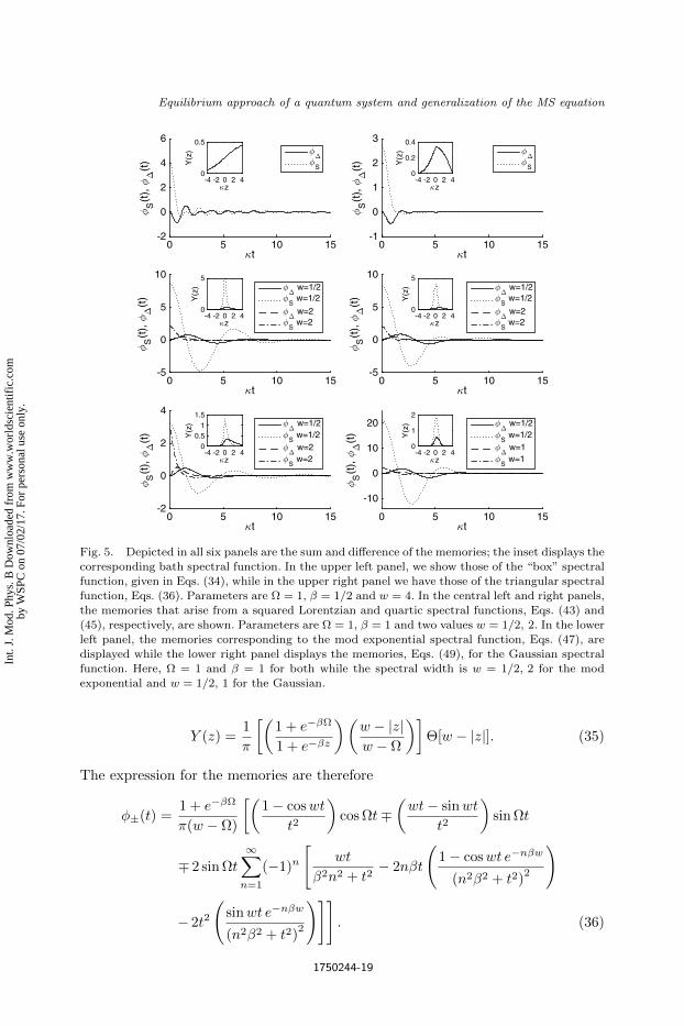
where Θ(z) is the Heaviside step function. The memories are
φ±(t) =1 + e−βΩ
π
[sinwt
tcos Ωt∓ 1− coswt
tsin Ωt
∓ 2 sin Ωt
∞∑n=1
(−1)n[(
t
n2β2 + t2
)(1− e−nβw coswt)
−(
nβ
n2β2 + t2
)e−nβw sinwt
]]. (34)
The sum φS(t) = φ−(t) + φ+(t) and difference φ∆(t) = φ−(t) − φ+(t) of the
memories given by Eqs. (34) are depicted in the upper left panel of Fig. 5, while
the bath spectral function for the “box,” Eq. (33), is shown in the inset. The
chosen parameter values are: thermal energy β = 1/2, the characteristic system
energy Ω = 1 and the spectral width w = 4. The discontinuous spectrum results in
memories with persistent oscillations.
The triangular spectral function is centered at the origin with width 2w, height
w/(w − Ω) and constant slope. The bath spectral function is given by
1750244-18
Int.
J. M
od. P
hys.
B D
ownl
oade
d fr
om w
ww
.wor
ldsc
ient
ific
.com
by W
SPC
on
07/0
2/17
. For
per
sona
l use
onl
y.
June 21, 2017 16:45 IJMPB S0217979217502447 page 19
Equilibrium approach of a quantum system and generalization of the MS equation
t0 5 10 15
S(t
),
(t)
-2
0
2
4
6
S
t0 5 10 15
S(t
),
(t)
-1
0
1
2
3
S
t0 5 10 15
S(t
),
(t)
-5
0
5
10 w=1/2
S w=1/2
w=2
S w=2
t0 5 10 15
S(t
),
(t)
-5
0
5
10 w=1/2
S w=1/2
w=2
S w=2
t0 5 10 15
S(t
),
(t)
-2
0
2
4 w=1/2
S w=1/2 w=2
S w=2
t0 5 10 15
S(t
),
(t)
-10
0
10
20 w=1/2
S w=1/2 w=1
S w=1
z-4 -2 0 2 4
Y(z
)
0
0.5
z-4 -2 0 2 4
Y(z
)
0
5
z-4 -2 0 2 4
Y(z
)
00.5
11.5
z-4 -2 0 2 4
Y(z
)
0
1
2
z-4 -2 0 2 4
Y(z
)
0
5
z-4 -2 0 2 4
Y(z
)
0
0.2
0.4
Fig. 5. Depicted in all six panels are the sum and difference of the memories; the inset displays thecorresponding bath spectral function. In the upper left panel, we show those of the “box” spectral
function, given in Eqs. (34), while in the upper right panel we have those of the triangular spectral
function, Eqs. (36). Parameters are Ω = 1, β = 1/2 and w = 4. In the central left and right panels,the memories that arise from a squared Lorentzian and quartic spectral functions, Eqs. (43) and
(45), respectively, are shown. Parameters are Ω = 1, β = 1 and two values w = 1/2, 2. In the lower
left panel, the memories corresponding to the mod exponential spectral function, Eqs. (47), aredisplayed while the lower right panel displays the memories, Eqs. (49), for the Gaussian spectral
function. Here, Ω = 1 and β = 1 for both while the spectral width is w = 1/2, 2 for the mod
exponential and w = 1/2, 1 for the Gaussian.
Y (z) =1
π
[(1 + e−βΩ
1 + e−βz
)(w − |z|w − Ω
)]Θ[w − |z|]. (35)
The expression for the memories are therefore
φ±(t) =1 + e−βΩ
π(w − Ω)
[(1− coswt
t2
)cos Ωt∓
(wt− sinwt
t2
)sin Ωt
∓ 2 sin Ωt
∞∑n=1
(−1)n
[wt
β2n2 + t2− 2nβt
(1− coswt e−nβw
(n2β2 + t2)2
)
− 2t2
(sinwt e−nβw
(n2β2 + t2)2
)]]. (36)
1750244-19
Int.
J. M
od. P
hys.
B D
ownl
oade
d fr
om w
ww
.wor
ldsc
ient
ific
.com
by W
SPC
on
07/0
2/17
. For
per
sona
l use
onl
y.

June 21, 2017 16:45 IJMPB S0217979217502447 page 20
V. M. Kenkre & M. Chase
The upper right panel of Fig. 5, depicts the sum and difference of the memories,
Eqs. (34), for the triangular spectra while the spectral function, Eq. (33), is in the
inset. Parameter values are Ω = 1, β = 1/2 and w = 4. Compared to the memories
that result from the “box” spectral function, those of the triangular Y (z) have
weaker oscillations; however, in both cases, the sharp truncation causes persistent
oscillations.
4.3.2. Spectral functions with infinite support
The Lorentzian spectral function, centered at the origin with spectral width w,
results in memories that are particularly simple. The normalized expression for the
bath spectral function is given by
Y (z) =
(1
π
)(1 + e−βΩ
1 + e−βz
)[Ω2 + w2
z2 + w2
]. (37)
The expressions for the memories that result from Eq. (37) are
φ±(t) =
(1 + e−βΩ
2
)(Ω2 + w2
w
)[(cos Ωt∓ tan
βw
2sin Ωt
)e−wt
∓ 4 sin Ωt
∞∑n=0
[βw
β2w2 − π2(2n+ 1)2
]e−π(2n+1)t
β
]. (38)
Figure 6, in its left panel, depicts the sum and difference of the memories, Eq. (38),
for two sets of the parameter values: characteristic system energy Ω = 1, thermal
energy β = 1 and spectral widths w = 1/4 and 4. An increase in the spectral
width leads to an increase in the damping of the memories. The inset displays
Lorentzian spectral functions that correspond to the characteristic energies above.
They are represented by solid and dashed-dotted lines, respectively. An increase in
the spectral width both broadens and shifts the bath spectral function.
The Lorentzian spectral function, Eq. (37), can be approximated for small values
of βw by a shifted Lorentzian with shift parameter z = βw/4. The width of the
approximated Lorentzian spectral function Y a(z) is modified such that w → w(1−z2). It is then given by
Y a(z) =
(1 + e−βΩ
2π
)Ω2 + w2
(z − wz)2 + w2(1− z2)2. (39)
The approximate spectra from Eq. (39) have been introduced because they lead
to memories φa±(t) that are somewhat simpler than the true memories, Eqs. (38).
They are given by
φa±(t) =
(1 + e−βΩ
2
)(Ω2 + w2
w(1− z2)
)cos (Ω± wz)t e−w(1−z2)t, (40)
and might be used for back-of-the-envelope calculations. The difference between the
real and approximate memories, Eqs. (38) and (40), respectively, is depicted in the
right panel of Fig. 6. Shown are φ∆(t)−φa∆(t) and φS(t)−φaS(t). The characteristic
1750244-20
Int.
J. M
od. P
hys.
B D
ownl
oade
d fr
om w
ww
.wor
ldsc
ient
ific
.com
by W
SPC
on
07/0
2/17
. For
per
sona
l use
onl
y.

June 21, 2017 16:45 IJMPB S0217979217502447 page 21
Equilibrium approach of a quantum system and generalization of the MS equation
t0 5 10 15
[-(t
)--a(t
)][
+(t
)-+a(t
)]
-0.2
-0.1
0
0.1
0.2
0.3
0.4
- a
S-
Sa
z-4 -2 0 2 4
Y(z
)-Y
a(z
)
-0.1
0
0.1
t0 5 10 15
S(t
),
(t)
-5
-4
-3
-2
-1
0
1
2
3
4
5
6
w=1/4
S w=1/4
w=4
S w=4
z-4 -2 0 2 4
Y(z
)
0
2
4
Fig. 6. The left panel displays the sum and the difference of the memories for a Lorentzian
spectral function, given in Eqs. (38). In the inset is the corresponding Y (z), Eq. (37). Here Ω = 1,β = 1 in both and two values of w = 1/4, 4 are shown. An increase in the spectral width leads to
a broadening of the spectrum (solid line in the inset) and an increase in the damping. Depicted in
the right panel are the difference between the real and approximated memories [φ−(t)− φa−(t)]−[φ+(t)− φa+(t)] for a single set of parameter values: Ω = 1, β = 1 and w = 1/4. In the inset is the
difference between the corresponding real and approximate bath spectral functions Y (z)−Y a(z).
Note the difference in scale for the left and right panels.
energies are taken to be the same as the first pair of memories (Ω = 1, β = 1 and
w = 1/4). The approximate bath spectral function, Eq. (39), differs from the true
Lorentzian spectral function closest to the origin (see inset of Fig. 6).
A generalization of the Lorentzian spectral function in Eq. (37) is the generalized
Cauchy distribution55 specified by the parameter ν which determines the high-
energy tails of the bath spectral function. The general expression is given by
Y (z; ν) =
(1
π
)(1 + e−βΩ
1 + e−βz
)[Ω2 + w2
z2 + w2
]ν, (41)
where ν > 1/2 is required for Y (z, ν) to be normalizable. The Lorentzian spec-
tral function, Eq. (37), re-emerges when ν = 1. Here, we give the case of ν = 2,
the square Lorentzian spectral function. This results in a z−4-dependence at high
energies. For this case, the generalized spectral function, Eq. (41), is specialized to
Y (z) =
(1
π
)(1 + e−βΩ
1 + e−βz
)[Ω2 + w2
z2 + w2
]2
. (42)
The memories that result from Eq. (42) are given by
φ±(t) =
(1 + e−βΩ
4
)(Ω2 + w2
w32
)2
×
[(1 + wt)(cos Ωt+ cos(Ωt± βw))± βw sin Ωt
1 + cosβwe−wt
∓ 8 sin Ωt
∞∑n=0
[β3w3
(β2w2 − π2(2n+ 1)2)2e−
π(2n+1)tβ
]]. (43)
1750244-21
Int.
J. M
od. P
hys.
B D
ownl
oade
d fr
om w
ww
.wor
ldsc
ient
ific
.com
by W
SPC
on
07/0
2/17
. For
per
sona
l use
onl
y.

June 21, 2017 16:45 IJMPB S0217979217502447 page 22
V. M. Kenkre & M. Chase
The bath spectral function, Eq. (42), and the sum and difference of the memories,
Eq. (43), are displayed in the central left panel of Fig. 5, for Ω = 1, β = 1 and
w = 1/2, 2. The bath spectral function (inset) shows the standard broadening and
shifting as the spectral width w is increased.
As a comparison, the quartic spectral function possesses a z−4-dependence at
high energies as well. The expression for its bath spectral function is
Y (z) =
(1
π
)(1 + e−βΩ
1 + e−βz
)[Ω4 + w4
z4 + w4
]. (44)
The distinction between the squared Lorentzian spectral function, Eq. (42), and
Eq. (44) is most evident in the intermediate energy regime. The memories that
result from Eq. (44) are given by
φ±(t) =
(1 + e−βΩ
√8
)(Ω4 + w4
w3
)[(cos
wt√2
+ sinwt√
2
)cos Ωt e
− wt√2
∓[(
sinh η + sin η
cosh η + cos η
)sin
wt√2−(
sinh η − sin η
cosh η + cos η
)cos
wt√2
]sin Ωt e
− wt√2
∓ 4√
2 sin Ωt∑n=0
[β3w3
β4w4 + π4(2n+ 1)4e−
π(2n+1)tβ
]]. (45)
Here η = βw/√
2. The sum and difference of the quartic spectral function memories,
Eqs. (43), are depicted for Ω = 1, β = 1 and w = 1/2 and 2 in the central right
panel of Fig. 5, with Y (z), Eq. (42), in the inset.
The mod exponential spectral function is centered at the origin with width w.
Its bath spectral function is given by
Y (z) =
(1
π
)(1 + e−βΩ
1 + e−βz
)e−|z|−Ωw . (46)
The memories that result from Eq. (46) are expressed as
φ±(t) =
(1 + e−βΩ
2π
)we
Ωw
[cos Ωt∓ wt sin Ωt
1 + w2t2
∓ 4 sin Ωt
∞∑n=1
(−1)nwt
(1 + nβw)2 + w2t2
](47)
The sum and difference of the memories, Eqs. (47), are depicted in the bottom left
panel of Fig. 5. The parameter values Ω = 1, β = 1 and two values of w = 1/2, 2
are considered. Inset is the mod exponential spectral function in dotted and solid
lines, respectively. The discontinuity in the derivative of the exponential spectral
function at z = 0 causes the oscillations to be persistent.
The final bath spectral function we consider is a Gaussian of width w already
referred to in our elucidation of temperature effects:
Y (z) =
(1
π
)(1 + e−βΩ
1 + e−βz
)e−
z2−Ω2
w2 . (48)
1750244-22
Int.
J. M
od. P
hys.
B D
ownl
oade
d fr
om w
ww
.wor
ldsc
ient
ific
.com
by W
SPC
on
07/0
2/17
. For
per
sona
l use
onl
y.

June 21, 2017 16:45 IJMPB S0217979217502447 page 23
Equilibrium approach of a quantum system and generalization of the MS equation
The magnitude of Eq. (48) is strongly dependent on the width. The memories that
result from a Gaussian spectral function are given by
φ±(t) =1 + e−βΩ
4
weΩ2
w2
√π
[e−
w2t2
4 cos Ωt± i(
w
(wt
2
)− w
(−wt
2
))sin Ωt
+ 2i sin Ωt∑n=1
(−1)n(
w
(wt+ inβw
2
)− w
(−wt+ inβw
2
))]. (49)
The Fourier transform of Eq. (48) results in a scaled error function of complex
argument which we represent with the Faddeeva function,58 w(iz) = exp(z2)erfc(z).
The presence of i in Eq. (49) should not lead the reader to conclude the memories
have imaginary components. As shown in the bottom right panel of Fig. 5, they
are certainly real. Depicted are the sum and difference of the memories for Ω = 1,
β = 1 and two values of w = 1/2 and 1 with the corresponding Y (z) inset with,
respectively, dotted and solid lines.
When the dimensionless energy ratio βw is small, the Gaussian spectral function
can be approximated with a shifted Gaussian centered at w(1−z2) where z = βw/4.
The approximation to the bath spectral function, Eq. (48), is given by
Y a(z) =1
π
1 + e−βΩ
2e−
Ω2
w2 e− (z−wz)2
w2(1−z2)2 . (50)
The exact memories for the approximate spectral function, Eq. (50), provide an
analytically tractable approximation for calculations. They are given by
φa±(t) =w(1− z2)√
π
1 + e−βΩ
2e
Ω2
w2 cos (Ω± wz)t e−w2(1−z2)2t2 (51)
4.4. Physical discussion of memory behavior
The behavior of the memories for particular bath spectral functions is intimately
related to the relative values of the three (dimensionless) energies that character-
ize the system and the reservoir: the system energy Ω, the thermal energy of the
bath 1/β and w, the energy that characterizes the spectral resolution of the bath.
Physically, the effects caused by the variation of these parameters are related to the
change in the ratios of the energy scales, βw, βΩ and Ω/w. The first ratio compares
the thermal energy of the reservoir to its average spectral energy. The second and
third ratios compare the respective reservoir energies to the system energy. Small
values of either lead to incoherent motion. The exchange of energy is suppressed
when the ratios are large, which extends the time scale of coherent system evolution.
It may be useful to discuss the effects on the memories directly in terms of
changes in the underlying energies. We do this in Figs. 7–9. In all the three figures,
we display the memories that result from a Lorentzian spectral function, Eq. (37),
and have set the time scale with κ.
In Fig. 7, we display the effects of varying the characteristic energy of the system
Ω on the memories. Two values, Ω = 1/2 and Ω = 2, are shown for three pairs of
1750244-23
Int.
J. M
od. P
hys.
B D
ownl
oade
d fr
om w
ww
.wor
ldsc
ient
ific
.com
by W
SPC
on
07/0
2/17
. For
per
sona
l use
onl
y.

June 21, 2017 16:45 IJMPB S0217979217502447 page 24
V. M. Kenkre & M. Chase
t0 10 20
(t)/
(0)
-0.8
-0.6
-0.4
-0.2
0
0.2
0.4
0.6
0.8
1
1.2
w=1/64
+ =1/2
- =1/2
+ =2
- =2
t0 2 4 6 8
(t)/
(0)
-0.4
-0.2
0
0.2
0.4
0.6
0.8
1w=1
+ =1/2
- =1/2
+ =2
- =2
t0 2 4 6 8
(t)/
(0)
-0.2
0
0.2
0.4
0.6
0.8
1w=64
+ =1/2
- =1/2
+ =2
- =2
Fig. 7. The normalized memories, φ±(t)/φ±(0), for the Lorentzian spectral function are shown
for two values of Ω in each of the panels. From left to right, the ratio of the characteristic reservoirenergies, βw, takes the values βw = 1/64 (β = 1/8, w = 1/8), βw = 1 (β = 1, w = 1) and
βw = 64 (β = 8, w = 8). The increase in Ω increases the oscillation frequency of the memories
and, therefore, the coherence time of the system evolution.
t0 5 10
(t)/
(0)
-0.8
-0.6
-0.4
-0.2
0
0.2
0.4
0.6
0.8
1
1.2
+ w=1/2
- w=1/2
+ w=2
- w=2
t0 5 10
(t)/
(0)
-0.6
-0.4
-0.2
0
0.2
0.4
0.6
0.8
1
+ w=1/2
- w=1/2
+ w=2
- w=2
t0 5 10
(t)/
(0)
-0.4
-0.2
0
0.2
0.4
0.6
0.8
1
+ w=1/2
- w=1/2
+ w=2
- w=2
Fig. 8. A variation to the spectral energy, at w = 1/2, 2, is displayed for the case of the Lorentzian
spectral function. Three pairs of the ratio of the characteristic system energy to the thermal energyof the reservoir are shown: (Ω = 8, β = 1/4), (Ω = 2, β = 1) and (Ω = 1/4, β = 8). The ratio
βΩ = 2 is held constant. An increase in the spectral width w generally results in an increase in
the damping relative to the oscillation period. However, smaller values of βw decrease the effectas the thermal energy scale begins to dominate the dynamics.
1750244-24
Int.
J. M
od. P
hys.
B D
ownl
oade
d fr
om w
ww
.wor
ldsc
ient
ific
.com
by W
SPC
on
07/0
2/17
. For
per
sona
l use
onl
y.

June 21, 2017 16:45 IJMPB S0217979217502447 page 25
Equilibrium approach of a quantum system and generalization of the MS equation
t0 2 4
(t)/
(0)
-0.6
-0.4
-0.2
0
0.2
0.4
0.6
0.8
1=1/2=2
t0 5 10
(t)/
(0)
-0.4
-0.2
0
0.2
0.4
0.6
0.8=1/2=2
t0 10 20
(t)/
(0)
-0.1
-0.05
0
0.05
0.1
0.15
0.2
0.25
0.3=1/2=2
Fig. 9. We display here the difference between the normalized memories, φ−(t)/φ−(0) −φ+(t)/φ+(0), against the dimensionless time κt for two values of the thermal energy, β = 1/2, 2,and three pairs of the ratio of the system energy and spectral width: left (Ω = 8, w = 48), center
(Ω = 2, w = 1) and right (Ω = 1/4, w = 1/8). Larger values of β result in an increase in the dis-
tinction between the memories. However, the effect itself becomes less important as βw decreasescommensurately with the increase in the spectral damping.
characteristic reservoir energies: β = 1/8 and w = 1/8 (left), β = 1 and w = 1
(center) and β = 8 and w = 8 (right). The characteristic reservoir energies are
chosen to highlight the effect of thermal deviations to the spectra. Generally, an
increase of Ω leads to a decrease in the period of oscillation. The left panel displays
the parameter regime where neither of the characteristic reservoir energy scales are
large compared to the system energy. Thus, the oscillation of the memories persist
for multiple periods. An increase to the characteristic reservoir energies, shown in
the second panel, results in an increase to the damping strength. However, as seen
in the right panel, when βw is large, thermal effects dominate the spectral energies
and coherency begins to re-emerge.
The memories for two values of the characteristic spectral energy, w = 1/2, 2,
are displayed in each panel of Fig. 8. The ratio of the characteristic system energy to
the thermal energy is held constant: left (Ω = 8, β = 1/4), center (Ω = 2, β = 1) and
right (Ω = 1/4, β = 8). As evidenced in Fig. 8, the coherent time scale is decreased
when the spectral width w is increased. Small values of w indicate a limit to the
capability of the reservoir to dissipate energy. The effect is diminished for small
values of βw when the thermal energy scale dominates the behavior of the reservoir.
Figure 9 depicts the effect of a change in β on the difference between the nor-
malized memories φ±(t)/φ±(0). This reflects the distinction between transitions to
sites at lower energy to those at higher energy. Each panel displays the difference
for two values, β = 1/2, 2, while the ratio of the characteristic system energy to
the spectral energies is held constant. From left to right, we use (Ω = 8, w = 4),
(Ω = 2, w = 1) and (Ω = 1/4, w = 1/8). An increase in the thermal energy leads to
1750244-25
Int.
J. M
od. P
hys.
B D
ownl
oade
d fr
om w
ww
.wor
ldsc
ient
ific
.com
by W
SPC
on
07/0
2/17
. For
per
sona
l use
onl
y.

June 21, 2017 16:45 IJMPB S0217979217502447 page 26
V. M. Kenkre & M. Chase
a commensurate increase in the distinguishability of the two memories. However,
this effect is damped when the spectral energy scale sets the energy of the reservoir,
i.e., when βw is large.
5. Conclusion
Although the analysis reported in this paper targets fundamental questions regard-
ing the approach to equilibrium of any quantum system, its aim is modest. It is not
to introduce the generalized master equation or solve the central problem of irre-
versibility or make understandable closure in nonequilibrium statistical mechanics,
all of which have been done (or attempted with a great deal of success) decades ago
by masters of the field.34–43 Even applications of the GME, particularly for trans-
port, have been systematically pursued as in the large body of work accumulated in
Frenkel exciton transport in molecular crystals.59 The focus of the present investi-
gation is rather on describing the approach to equilibrium with particular attention
paid to the simultaneous occurrence of decoherence and population relaxation; and
to use for this purpose simple GMEs obtained in the weak-coupling approximation.
The use of the weak-coupling approximation here should be noted as a desirable
feature rather than a source of apology since, as explained in Sec. 1, the interaction
with the bath that one must select is necessarily such that no superfluous signatures
of the bath are left in the final state. That final equilibrium state must be given
by the double postulate of equilibrium statistical mechanics (that has no reference
to the bath other than the value of the temperature, only to the eigenstates of the
system) as explained in textbooks.21
An analysis similar to the one reported here was initiated briefly in a previ-
ous publication50 where the system was rather elementary, a nonresonant dimer
(two-state system with unequal energies of the states). The present study targets
considerably more realistic systems: a harmonic oscillator representing a molecule
undergoing vibrational relaxation (Sec. 3) and a charged particle moving in a crys-
tal lattice made energetically nondegenerate by the application of a strong electric
field. Our study of the first system provides a GME generalization of the well-known
Montroll–Shuler equation9 in chemical physics and thereby extends its applicability
to very short times and opens the possibility of practical application in those time
ranges.
That work on vibrational relaxation, particularly at short times, reported in
Sec. 2 of this paper, is the primary practical goal of our investigation. Recent
availability of experimental methods capable of probing the process of vibrational
relaxation at shorter and shorter times (the passage of pico- into femto-spectroscopy
and now the advent of even faster spectroscopy) should make our study especially
relevant in the modern era. We mention, as examples, the work of Zewail and collab-
orators: femtosecond observation of coherent collisional confinement,25 of solvated
oxygen anions26 and of anomalies in the vibrational redistribution in azulene.27
1750244-26
Int.
J. M
od. P
hys.
B D
ownl
oade
d fr
om w
ww
.wor
ldsc
ient
ific
.com
by W
SPC
on
07/0
2/17
. For
per
sona
l use
onl
y.

June 21, 2017 16:45 IJMPB S0217979217502447 page 27
Equilibrium approach of a quantum system and generalization of the MS equation
Specifically, we have generalized the Montroll–Shuler equation (4), a respected
workhorse of traditional vibrational relaxation investigations, into the GME (6)
along with explicit prescriptions to obtain the memory functions φ±(t) from fea-
tures of the bath with which the relaxing molecule interacts. The bath features
are to be found in the spectral function Y (z). The Fourier-transform prescription
obtained by generalizing Zwanzig’s projection operators to include coarse-graining
is explained in Appendix A and a treatment cataloging various spectral functions
and consequent memories by the application of that prescription are provided in
Sec. 4. Section 2.3 and Fig. 1 make particularly clear how our theoretical predictions
may be compared, in principle, to coherent observations of vibrational relaxation
at ultra-short times.
While not the primary goal of our analysis in this paper, the charge in the
crystal lattice analyzed in Sec. 3 is a secondary target of our study, included here
as it is naturally studied with our methods. It can be viewed as a system that
generalizes the elementary example of the nonresonant dimer analyzed by Tiwari
and Kenkre50 by augmenting its two states into an infinite number of states (sites
of the crystal). The vibrational relaxation of the molecule analyzed in Sec. 2 is
a similar generalization to a semi-infinite number of states (appropriate to the
harmonic oscillator spectrum) starting from two in the simple system of Ref. 50
but also with the added complication of the site-dependent matrix elements of
the bath interaction Hamiltonian. Our study of the charge under the action of an
electric field in a crystal lattice uncovers an interesting transition from coherent
behavior at short times, characterized by localization around the initial state, to
delocalization at long times as the charge escapes to infinitely distant sites. This is
a passage from quantum mechanical motion to classical motion.
The study of several cases of the phenomenological bath is another feature of the
present paper. We have calculated the memory functions of our GME for various re-
alizations of the spectral bath function Y (z) and investigated the dependence of the
memory functions on the temperature as well as spectral features. The advantage
of using phenomenologically modeled baths and consequent spectral functions, as
we have done in the present paper, is that it allows the study of complex reservoir
interactions which are difficult to model simply but are reflected in independent
observations. This is best exemplified by the Forster prescription in the theory
of energy transfer60 where the independent observations are absorption and emis-
sion spectra while the phenomena that need to be described are those involving
excitation transfer.
Nevertheless, it is also possible to show how to obtain our GME and the mem-
ory functions in it directly for fully specified microscopic models. In cases wherein
the interaction term in equations such as Eqs. (A.3) and (A.4) is of the product
form V = VSVB , where the first (second) factor has operators only of the system
(bath), the memories can be simplified further. As in Ref. 16, the memory functions,
WMN (t) and WNM (t), can be written as products of pure system factors and pure
1750244-27
Int.
J. M
od. P
hys.
B D
ownl
oade
d fr
om w
ww
.wor
ldsc
ient
ific
.com
by W
SPC
on
07/0
2/17
. For
per
sona
l use
onl
y.

June 21, 2017 16:45 IJMPB S0217979217502447 page 28
V. M. Kenkre & M. Chase
bath correlations B(t) = 〈VBV †B(t)〉 and its complex conjugate B∗(t) = 〈VB(t)V †B〉:
WMN (t) = |〈M |VS |N〉|2(eiΩMN tB(t) + e−iΩMN tB∗(t)), (52a)
WNM (t) = |〈M |VS |N〉|2(e−iΩMN tB(t) + eiΩMN tB∗(t)). (52b)
Here ΩMN = EM − EN/~ is the frequency defined by the energy difference
between the system energy levels M and N ; and |〈M |VS |N〉|2 depends only on
the system (not bath). In the case of the degenerate system (no differences in the
energies between states, i.e., ΩMN = ΩNM = 0), the memory functions are found
to be equal to each other,
WMN (t) =WNM (t) = |〈M |VS |N〉|2(B(t) + B∗(t)). (53)
The bath correlation functions B(t) and B∗(t) involve symbols such as 〈· · · 〉and VB(t). These follow the standard notation in textbooks and represent, respec-
tively, the bath thermal average and the Heisenberg time dependence, HB being
the Hamiltonian of the bath. Thus
B(t) = 〈VBV †B(t)〉 =Tr(e−βHBVBe
itHBV †Be−itHB )
Tr(e−βHB ). (54)
Work with the help of the theory developed here is under way in several further
directions. One of them focuses on calculations of the memories and the study of
the short-time aspects of relaxation for microscopically specified baths via computa-
tions of the correlation function given by Eq. (54) appropriate to observations.4–6,16
Quantum representations of anharmonic reservoirs are also being studied in this
context.61 Another elucidates the effects of initial conditions of molecular exci-
tation or system preparation as described by driven GMEs. Such a treatment is
necessary because the analysis we have given here is only applicable for an initial
density matrix that is random in the representation of M , N , etc. For situations
in which this is not true, the GME must be supplemented by driving terms first
derived long ago by van Hove,34 Zwanzig35 and others and analyzed in specific con-
texts.44 Yet other directions of our current research focus on the understanding of
time-independent aspects of relaxation observations such as the puzzling inverted
temperature dependence of rates reported by Tokmakoff and collaborators.5 These
matters, available in the form of unpublished calculations, will be the contents of
a future publication.62
Acknowledgments
It is a pleasure to acknowledge helpful discussions with Anastasia Ierides.
Appendix A. Essentials of the Fourier-Transform Prescription
to Obtain Coarse-Grained Memories
A minimal description of how to obtain the Fourier-transform prescription45 origi-
nally given by one of the present authors is provided in this Appendix to facilitate
1750244-28
Int.
J. M
od. P
hys.
B D
ownl
oade
d fr
om w
ww
.wor
ldsc
ient
ific
.com
by W
SPC
on
07/0
2/17
. For
per
sona
l use
onl
y.

June 21, 2017 16:45 IJMPB S0217979217502447 page 29
Equilibrium approach of a quantum system and generalization of the MS equation
an understanding of the derivation. This appears useful because the original expo-
sition48 had been in the context of the extension into the coherent domain of the
Forster theory60 of excitation transfer in photosynthetic and related systems and
had a sharply specialized emphasis. The derivation uses coarse-grained projection
operators introduced as a generalization45,48,49 to the diagonalization projection
operators invented in Refs. 35–38. Starting with the von Neumann equation for the
density matrix ρ, we arrive under the guidance of the Zwanzig procedure at the
master equation for the probabilities. However, the latter are coarse-grained enti-
ties characteristic only of the system, rather than of the system–bath composite,
and obtained through a summation over the states of the bath. The summation
is built45,48,49 into the projection operator. Specifically, if M , N , etc. denote the
states of the system alone and m, n, p, etc. denote those of the bath, the projection
operator P is defined to act on any operator O, as
〈M,m|PO|N,n〉 =QmQ
[∑p
〈M,p|O|M,p〉
]δM,Nδm,n. (A.1)
Its action is threefold. The two Kronecker deltas correspond to the fact that PO is
diagonal. The sum coarse-grains over the bath states. Each microstate is weighted
through a factor Qm, idempotency of P being ensured by the normalization∑mQm = Q. As explained elsewhere,49 different realizations of the weighting factor
Qm may be used in the coarse-graining for different goals but here we take them as
corresponding to the bath thermal distribution proportional to e−βεm . The energy
of the mth bath eigenstate is denoted by εm, and as elsewhere, β is the dimension-
less inverse temperature. The rest of the calculation follows Zwanzig’s in its essence
but removes an important shortcoming by introducing sums over bath states in the
very prescription for the memories thereby providing a Fourier-transform recipe to
obtain memories from bath spectral functions. We obtain Zwanzig’s GME as
dPM (t)
dt=∑N
∫ t
0
dt′[WMN (t− t′)PN (t′)−WNM (t− t′)PM (t′)], (A.2)
where WMN (t) and WNM (t) are the memories but now directly between coarse-
grained states M and N , rather than between single states of the system–bath
combination. The memories are given by
WMN (t) = 2∑m,n
e−βεn
Z|〈M,m|V |N,n〉|2 cos [(εmn + EMN )t], (A.3a)
WNM (t) = 2∑m,n
e−βεm
Z|〈M,m|V |N,n〉|2 cos [(εmn + EMN )t], (A.3b)
where EMN = EM − EN and εmn = εm − εn are the differences in energy be-
tween the system states and bath states, respectively, and Z =∑n e−βεn is the
bath partition function. To get Eq. (A.3b), whose only difference from Eq. (A.3a)
is the presence of εm rather than of εn in the Boltzmann weighting factor within the
1750244-29
Int.
J. M
od. P
hys.
B D
ownl
oade
d fr
om w
ww
.wor
ldsc
ient
ific
.com
by W
SPC
on
07/0
2/17
. For
per
sona
l use
onl
y.

June 21, 2017 16:45 IJMPB S0217979217502447 page 30
V. M. Kenkre & M. Chase
bath summation, we first switch in Eq. (A.3a) labels N with M and n with m and
then use the indifference of cosine to the sign of its argument. These expressions
correspond with the textbook statement that one performs a thermal average over
initial states and a sum over the final states.
We can now again switch indices within the bath summation, use the properties
of the cosine and write Eq. (A.3b) in the form
WNM (t) = 2∑m,n
e−βεn
Z|〈M,m|V |N,n〉|2 cos [(εmn − EMN )t]. (A.4)
The distinction between the two memories connecting the coarse-grained states M–
N is then wholly in a sign in the argument of the cosine. The memory corresponding
to the transition from N to M has the difference of εmn and EMN whereas that
corresponding to the transition from M to N has their sum.
Consider now a complex system wherein the bath energy differences may be
regarded as continuous and denoted by the variable z. We split the unrestricted
summation∑m,n over the bath states into a primed (restricted) summation
∑′m,n
with the restriction that εmn equals the value z, followed by an integration over the
latter. Equations (A.3) may be written more appropriately in the integral form
WMN (t) =
∫ ∞−∞
dz YMN (z) cos [(z + EMN )t], (A.5a)
WNM (t) =
∫ ∞−∞
dz e−βzYNM (z) cos [(z + EMN )t], (A.5b)
with Eq. (A.4) becoming
WNM (t) =
∫ ∞−∞
dz YMN (z) cos [(z − EMN )t]. (A.6)
Several features deserve mention. The quantities YMN (z) and YNM (z) con-
tain everything in the summands except the cosines, thus YMN (z) =
2[ρ(z)/Z]∑′
m,n e−βεn |〈M,m|V |N,n〉|2, the factor e−βz in the second equation ap-
pears because of the switch of m and n in the indices in the summands and ρ(z)
is the density of states that emerges from the replacement of the summation by an
integration.
In systems such as the ones analyzed here, YMN (z) or YNM (z) are separable
into a product of a system expression and a bath expression. Thus, for the primary
situation analyzed in Sec. 2 of the main paper, the harmonic oscillator in interaction
with the bath, the system expression is proportional to
[√M + 1δN,M+1 +
√MδN,M−1]2 = (M + 1)δN,M+1 +MδN,M−1.
The expression is a consequence of the square root dependence of the matrix ele-
ment of the system–bath interaction between harmonic oscillator eigenstates and
its nearest-neighbor nature in the M,N -space. This is so because the interaction is
linear in the oscillator coordinate from the Taylor expansion employed by Landau
1750244-30
Int.
J. M
od. P
hys.
B D
ownl
oade
d fr
om w
ww
.wor
ldsc
ient
ific
.com
by W
SPC
on
07/0
2/17
. For
per
sona
l use
onl
y.

June 21, 2017 16:45 IJMPB S0217979217502447 page 31
Equilibrium approach of a quantum system and generalization of the MS equation
and Teller.47 By contrast, the second system analyzed in the paper, in Sec. 3, the
charge under the action of an electric field in a crystal, the system expression of
YMN (z) or YNM (z) has no similar square root dependence on the system state label
but is taken nearest-neighbor and thus proportional simply to [δN,M+1 + δN,M−1].
The other factor in the expression for YMN (z) or YNM (z) comes from bath
properties. We denote it by Y (z) without the indices M and N , and call it the
bath spectral function Y (z). It allows one to focus attention on a phenomenolog-
ical construction of the bath used in the present paper. The equivalence between
Eqs. (A.5b) and (A.6) shown above is an explicit proof of the generalized detailed
balance requirement, given in Eq. (2) in the text, that Y (z) respects the relation
Y (−z) = e−βzY (z) given in the text or that it can always be represented through
a symmetric function as in Eq. (3).
Finally, we can write down the YMN used in Sec. 2 as
YMN (z) =
[Ys(z)
1 + e−βz
][(M + 1)δN,M+1 +MδN,M−1], (A.7)
and that used in Sec. 3 as
YMN (z) =
[Ys(z)
1 + e−βz
][δN,M+1 + δN,M−1]. (A.8)
The transition rate κ is given by substituting z in κ = Ys(z)/(1 + e−βz) by Ω for
the harmonic oscillator case in Sec. 2 and E for the charge in the crystal case in
Sec. 3. The phenomenological introduction of any symmetric function for Ys(z),
with assumed z-dependence as discussed for various cases in Sec. 4, completes the
full specification of the GMEs, Eqs. (6) and (26), at the respective starting points
of Secs. 3 and 4.
References
1. A. Laubereau and W. Kaiser, Rev. Mod. Phys. 50, 605 (1978).2. S. H. Lin and H. Eyring, Annu. Rev. Phys. Chem. 25, 39 (1974).3. D. W. Oxtoby, Annu. Rev. Phys. Chem 32, 77 (1981).4. D. D. Dlott and M. D. Fayer, J. Chem. Phys. 92, 3798 (1990).5. A. Tokmakoff et al., Chem. Phys. Lett. 221, 412 (1994).6. A. Tokmakoff, B. Sauter and M. D. Fayer, J. Chem. Phys. 100, 9035 (1994).7. R. J. Rubin and K. E. Shuler, J. Chem. Phys. 25, 59 (1956); 25, 68 (1956).8. R. J. Rubin and K. E. Shuler, J. Chem. Phys. 26, 137 (1957).9. E. W. Montroll and K. E. Shuler, J. Chem. Phys. 26, 3 (1957).
10. A. Nitzan and J. Jortner, Mol. Phys. 25, 713 (1973).11. K. F. Freed and D. F. Heller, J. Chem. Phys. 61, 3942 (1974).12. D. J. Diestler, Adv. Chem. Phys. 35, 305 (1980).13. S. A. Adelman, R. Muralidhar and R. H. Stote, J. Chem. Phys. 95, 2738 (1991).14. V. M. Kenkre and V. Seshadri, Phys. Rev. A 15, 197 (1977).15. V. Seshadri and V. M. Kenkre, Phys. Rev. A 17, 223 (1978).16. V. M. Kenkre, A. Tokmakoff and M. D. Fayer, J. Chem. Phys. 101, 10618 (1994).17. F. P. Buff and D. J. Wilson, J. Chem. Phys. 32, 677 (1960).18. A. H. Zewail, J. Phys. Chem. A 104, 5660 (2000).
1750244-31
Int.
J. M
od. P
hys.
B D
ownl
oade
d fr
om w
ww
.wor
ldsc
ient
ific
.com
by W
SPC
on
07/0
2/17
. For
per
sona
l use
onl
y.

June 21, 2017 16:45 IJMPB S0217979217502447 page 32
V. M. Kenkre & M. Chase
19. K. E. Shuler, Symp. (Int.) Combust. 5, 56 (1955).20. A. Tokmakoff, M. D. Fayer and D. D. Dlott, J. Phys. Chem. 97, 1901 (1993).21. K. Huang, Statistical Mechanics (Wiley, New York, 1987) [see in particular pp. 172–
173].22. W. H. Zurek, S. Habib and J. P. Paz, Phys. Rev. Lett. 70, 1187 (1993).23. D. Giulini et al., Decoherence and the Appearance of a Classical World in Quantum
Theory (Springer, Berlin, 1996).24. W. H. Zurek, Rev. Mod. Phys. 75, 715 (2003).25. C. Wan et al., J. Chem. Phys. 106, 4353 (1997).26. E. W.-G. Diau, S. D. Feyter and A. H. Zewail, J. Chem. Phys. 110, 9785 (1999).27. N. J. Kim, D. H. Paik and A. H. Zewail, J. Chem. Phys. 118, 6930 (2003).28. S. K. Sundaram and E. Mazur, Nature Mater. 1, 217 (2002).29. E. Goulielmakis et al., Nature 466, 739 (2010).30. I. Tehver and V. Hizhnyakov, Zh. Eksp. Teor. Fiz. 69, 599 (1975) [English translation:
Sov. Phys.-JETP 42, 305 (1976)].31. V. M. Kenkre, Phys. Rev. A 16, 766 (1977).32. H. C. Andersen et al., J. Math. Phys. 5, 522 (1964).33. H. C. Andersen et al., J. Chem. Phys. 41, 3012 (1964).34. L. van Hove, Physica 23, 441 (1957).35. R. Zwanzig, J. Chem. Phys. 33, 1338 (1960).36. R. Zwanzig, Lectures in Theoretical Physics, Vol. 3, eds. W. E. Brittin, B. W. Downs
and J. Downs (Interscience, New York, 1961).37. R. Zwanzig, Physica 30, 1109 (1964).38. R. Zwanzig, Statistical mechanics of irreversibility, in Quantum Statistical Mechanics,
ed. P. H. E. Meijer (Gordon and Breach, New York, 1966), p. 139.39. E. G. D. Cohen (ed.), Fundamental Problems in Statistical Mechanics: Proc. NUFFIC
Int. Summer Course in Science at Nijenrode Castle, the Netherlands, August, 1961,(North-Holland, Amsterdam, 1962).
40. J. de Boer and G. E. Uhlenbeck, Studies in Statistical Mechanics, Vol. 1 (North-Holland, Amsterdam, 1962).
41. E. W. Montroll, in Fundamental Problems in Statistical Mechanics, ed. E. G. D. Cohen(North-Holland, Amsterdam, 1962), p. 230.
42. I. Prigogine and P. Resibois, Physica 24, 795 (1958).43. R. J. Swenson, J. Math. Phys. 3, 1017 (1962).44. V. M. Kenkre, J. Stat. Phys. 19, 333 (1978).45. V. M. Kenkre, The generalized master equation and its applications, in Statistical Me-
chanics and Statistical Methods in Theory and Application, ed. U. Landman (PlenumPress, New York, 1977), p. 441.
46. H. A. Bethe and E. Teller, Deviations from thermal equilibrium in shock waves, ReportNo. X-117, Ballistic Research Laboratory, Maryland, USA (1941).
47. L. Landau and E. Teller, Phys. Z. Sowjetunion 10, 34 (1936).48. V. M. Kenkre and R. S. Knox, Phys. Rev. B 9, 5279 (1974).49. V. M. Kenkre, Phys. Rev. B 11, 3406 (1975).50. M. Tiwari and V. M. Kenkre, Eur. Phys. J. B 87, 1 (2014).51. G. H. Wannier, Rev. Mod. Phys. 34, 645 (1962).52. J. B. Krieger and G. J. Iafrate, Phys. Rev. B 33, 5494 (1986).53. C. A. Moyer, J. Phys. C 6, 1461 (1973).54. D. Emin and C. F. Hart, Phys. Rev. B 36, 2530 (1987).55. P. R. Rider, Ann. Inst. Stat. Math. 9, 215 (1957).56. H. C. Wolf, Energy transfer in organic molecular crystals: A survey of experiments, in
1750244-32
Int.
J. M
od. P
hys.
B D
ownl
oade
d fr
om w
ww
.wor
ldsc
ient
ific
.com
by W
SPC
on
07/0
2/17
. For
per
sona
l use
onl
y.
June 21, 2017 16:45 IJMPB S0217979217502447 page 33
Equilibrium approach of a quantum system and generalization of the MS equation
Advances in Atomic and Molecular Physics, Vol. 3, eds. D. R. Bates and I. Eastermann(Academic Press, New York, 1967), pp. 119–142.
57. R. C. Powell and Z. G. Soos, J. Lumin. 11, 1 (1975).58. M. Abramowitz and I. E. Stegun, Handbook of Mathematical Functions (Dover,
Toronto, 1970).59. V. M. Kenkre and P. Reineker, Exciton Dynamics in Molecular Crystals and Aggre-
gates, ed. G. Hoehler, Springer Tracts in Modern Physics, Vol. 94 (Springer, Berlin,1982).
60. T. Forster, Ann. Phys. 2, 55 (1948).61. D. P. Visco, Jr. and S. Sen, Phys. Rev. E 57, 225 (1998); 58, 1419 (1998).62. A. A. Ierides and V. M. Kenkre, Analysis of Inverted Temperature Dependence of
Vibrational Relaxation Rates in Molecules Embedded in a Bath, University of NewMexico, preprint (2017).
1750244-33
Int.
J. M
od. P
hys.
B D
ownl
oade
d fr
om w
ww
.wor
ldsc
ient
ific
.com
by W
SPC
on
07/0
2/17
. For
per
sona
l use
onl
y.