APPROXIMATE KNOWLEDGE OF

RATIONALITY AND CORRELATED EQUILIBRIA

by

Fabrizio Germano and Peio Zuazo-Garin

2012

Working Paper Series: IL. 61/12

Departamento de Fundamentos del Análisis Económico I

Ekonomi Analisiaren Oinarriak I Saila

University of the Basque Country

Approximate Knowledge of Rationality and

Correlated Equilibria∗

Fabrizio Germano† and Peio Zuazo-Garin‡

July 16, 2012

Abstract

We extend Aumann’s [3] theorem deriving correlated equilibria as a consequence of common priors

and common knowledge of rationality by explicitly allowing for non-rational behavior. We replace the

assumption of common knowledge of rationality with a substantially weaker notion, joint p-belief of

rationality, where agents believe the other agents are rational with probabilities p = (pi)i∈I or more.

We show that behavior in this case constitutes a constrained correlated equilibrium of a doubled game

satisfying certain p-belief constraints and characterize the topological structure of the resulting set of p-

rational outcomes. We establish continuity in the parameters p and show that, for p sufficiently close to

one, the p-rational outcomes are close to the correlated equilibria and, with high probability, supported

on strategies that survive the iterated elimination of strictly dominated strategies. Finally, we extend

Aumann and Dreze’s [4] theorem on rational expectations of interim types to the broader p-rational

belief systems, and also discuss the case of non-common priors.

Keywords: Correlated equilibrium, approximate common knowledge, bounded rationality, p-rational

belief system, common prior, information, noncooperative game. JEL Classification: C72, D82, D83.

“Errare humanum est, perseverare diabolicum.”

1 Introduction

Rationality, understood as consistency of behavior with stated objectives, information, and strategies avail-

able, naturally lies at the heart of game theory. In a celebrated paper, [3], Aumann takes as point of

∗We are indebted to Bob Aumann, Eddie Dekel, Sergiu Hart, and Dov Samet, for valuable comments and conversations.Germano acknowledges financial support from the Spanish Ministry of Science and Technology (Grants SEJ2007-64340 andECO2011-28965), as well as from the Barcelona GSE Research Network and the Generalitat de Catalunya. Zuazo-Garinacknowledges financial support from the Spanish Ministry of Science and Technology (Grant ECO2009-11213), and inestimablehelp from professors Elena Inarra and Annick Laruelle, and from Jeon Hyang Ki. Both authors also thank the Center for theStudy of Rationality at the Hebrew University of Jerusalem for their generous support and hospitality. All errors are our own.†Universitat Pompeu Fabra, Departament d’Economia i Empresa, and Barcelona GSE, Ramon Trias Fargas 25-27, E-08005

Barcelona, Spain; fabrizio.germano@upf.edu.‡BRiDGE, Universidad del Paıs Vasco, Departamento de Fundamentos del Analisis Economico I, Avenida Lehendakari

Aguirre 83, E-48015, Bilbao, Spain; peio.zuazo@ehu.es.

1

departure the rationality of all agents in any state of the world, knowledge thereof, as well as the existence of

a common prior, to show that joint play by the players of the game will necessarily conform to a correlated

equilibrium.

Given that the objectives, strategies and information structure are part of the description of the game or

game situation at hand, they are relatively flexible restrictions and indeed in many cases should be adaptable

to the actual underlying game. Nonetheless it is both possible and plausible that agents may deviate from

a complete consistency with the assumed restrictions. This can happen in many ways as agents can make

mistakes at any stage of participating in the game situation:1 they can make a mistake in perceiving or

interpreting their objective (e.g., a trader may apply a wrong set of exchange exchange rates when deciding

a transaction), they may make a mistake in carrying out the selected strategy (e.g., a soccer player may trip

or make a wrong step when shooting a penalty kick), they may make a mistake in processing their available

information (e.g., a judge may forget to consult a crucial, requested technical report when deciding on a

specific court case) and so on. It is clear that departures from full rationality not only occur, occur often,

but also occur in innumerable ways.

In this paper, we build on the approach of [3] in formalizing the overall strategic interaction, but depart

from it by allowing agents to entertain the possibility that other agents may not always be consistent.

Specifically, we assume that agents believe that the other agents are rational with probability pi and that

with the remaining probability (1 − pi or less) they are not rational. In doing so we put as little structure

as possible on what it means to be not rational, except that the rules of the game force agents to select

some action in the game. This is in line with our belief that when modeling “social behavior” very broadly

defined, mistakes or inconsistencies not only occur but also occur in innumerable ways. Therefore, without

imposing assumptions on the kind of deviations from rational play that players may make, except that

its probability of occurrence is limited by some vector p, and maintaining the common prior assumption

(common to all types of agents), we explore the consequences of what we call joint p-belief of rationality.

The two assumptions together, common prior and joint p-belief of rationality, are what we call p-rationality,

for p ∈ [0, 1]I .

The main result of the paper, Theorem 1, then characterizes strategic behavior in games where players

are p-rational and share a common prior. This provides a generalization of [3], since our p-rational outcomes

collapse to the correlated equilibria when p = 1. Our second result, Theorem 2, shows basic topological

properties of the p-rational outcomes, in particular convexity, compactness but, more importantly, also

that the set varies continuously in the underlining parameters p. We also show that when p = minp is

sufficiently close to 1, then strategy profiles involving strategies that do not survive iterated elimination of

strictly dominated strategies get probability at most p under the common prior. Following Aumann and

Dreze in [4], we also ask what payoffs agents should expect under p-rationality, and thus characterize in

Theorem 3, what we call p-rational expectations of interim types. Finally, we also briefly discuss the case of

1We refer to [9] and [16] for surveys on bounded rationality, and to [8] for a survey of behavioral game theory.

2

non-common priors and show that in this case, joint p-belief of rationality puts no restriction on behavior.

The paper only considers the case of complete information games.

Overall, the paper is structured as follows. Section 2 provides the basic definitions, Section 3 contains

the main results characterizing the p-rational outcomes and expectations, Section 4 provides some examples,

and Section 5 some concluding remarks. All proofs are relegated to the Appendix.

2 p-Rational Belief Systems

Our main object of study are what we define as p-rational belief systems. These generalize the rational belief

systems of [3], [4], and [10], and allow us to formalize a situation where there is no common knowledge of

rationality, but where players nonetheless believe, with probabilities above certain levels (p = (pi)i), that

the other players are rational. Following [4] and [10] we start by defining belief systems, which are more

basic and which play a central role throughout the paper. They encapsulate what players believe about the

game and about the other players.

2.1 Belief Systems

Throughout the paper we denote by G =⟨I, (Ai)i∈I , (hi)i∈I

⟩a finite game in strategic form defined the

usual way, with I a finite set of players; Ai player i’s set of pure strategies, which we also assume to be finite,

where A = Πi∈IAi and A−i = Πj∈I\{i}Aj ; and hi : A→ R player i’s payoff function.

Definition 1 (Belief System) A belief system for the game G is a triple B =⟨(Ti)i∈I , (si)i∈I , (fi)i∈I

⟩such that, for each player i ∈ I,

• Ti is a finite type set,

• si : Ti → Ai is a strategy map and

• fi ∈ ∆ (T ) is i’s prior, such that T =∏i∈ITi, has full marginal support in Ti.

We refer to any given element of T , t = (ti)i∈I , as a state of the world, or simply, state. Note that for each

player i ∈ I, the prior fi induces posteriors on other players’ types, conditional on i’s type:

fi (ti) (t−i) =fi (t−i; ti)

fi (T−i × {ti}), for any t−i ∈ T−i.

We say that B satisfies the common prior assumption, CP , if fi = fj for all i, j ∈ I, will denote them by

just f , will refer to the latter as the common prior and will represent B by⟨(Ti)i∈I , (si)i∈I , f

⟩. For any

state t = (t−i; ti), we say that player i is rational at t, if

si(ti) ∈ argmaxai∈Ai

EB (h (a−i; ai) |fi (ti)) ,

3

where EB (h (a−i; ai) |fi (ti)) =∑t−i∈T−i

fi(ti) (t−i)hi (s−i (t−i) ; si). We denote by Ri the set of states in

which player i is rational. Note that at any state t, player i being rational in this state only depends on the

i-th component of t, namely, player i’s type ti. This implies the following characterization,

Ri = T−i ×{ti ∈ Ti

∣∣∣∣ s(ti) ∈ argmaxai∈Ai

EB (hi (a−i; ai) |fi (ti))

}.

The set of the states in which every player but i is rational (without excluding i’s possible rationality),⋂j∈I\{i}Rj , will be denoted by R−i. By R, we will denote the set of states in which every player is rational.

We will say that a belief system B satisfies common knowledge of rationality, CK (R), if every player is

rational at every state, that is, if T = R.2

Finally, we say that a belief system is rational if it satisfies both CP and CK (R). It is well known from

[3] that the outcome distributions over the set of strategies of a finite game in strategic form G played under

some rational belief system B, are precisely the correlated equilibria of game G, which we denote by CE(G).

2.2 p-Belief Operators and p-Rationality

By an event we mean any subset E ⊆ T . Recall that, following [14], and making the corresponding adap-

tations to the setup in the previous section, for any given pi ∈ [0, 1], and any event E ⊆ T , we can define

player i’s pi-belief operator as,

Bpii (E) = T−i × {ti ∈ Ti | fi (ti) (E) ≥ pi } .

For any t ∈ T , any event E, and any pi ∈ [0, 1], we say that player i pi-believes E in t, if t ∈ Bpii (E). For

p = (pi)i∈I ∈ [0, 1]I , we say that an event E is p-evident if E ⊆⋂i∈I B

pii (E), and given any state t, we say

that an event C is common p-belief in t if there exists some p-evident event E such that t ∈ E ⊆⋂i∈I B

pii (C).

We denote the event that C is common p-belief by CBp(C). We say that a belief system B satisfies common

p-belief of rationality if T = CBp (R). Now, it is easy to see that common p-belief of rationality is satisfied

if and only if T =⋂i∈I B

pii (R), so the latter is, for convenience, the characterization of common p-belief

of rationality we will make use of through the paper.3 As T is finite, it is again easy to check that a belief

system satisfies 1-belief of rationality if and only if it satisfies common knowledge of rationality.

For reasons explained below, the following notion of approximate knowledge of rationality replaces the

notion of CK(R) assumed in [3] and elsewhere.

Definition 2 (Joint p-Belief of Rationality) A belief system B satisfies joint p-belief of rationality,

JpB (R), if T =⋂i∈I B

pii (R−i).

2As is shown in [14], p.174, this does indeed imply common knowledge of rationality. In this case, T is clearly such anevident knowledge, and, hence, also R.

3Despite not being true, in general for an event E, that CBp(E) =⋂

i∈I Bpii (E).

4

The following are basic results regarding relations between common knowledge of rationality, common p-

belief of rationality and JpB (R).

Lemma 1 Let G be a game and B a belief system for G, then:

(a) For any p ∈ (0, 1]I , if B satisfies CBp (R), then B satisfies CK (R), and is therefore, rational.

(b) For any p ∈ (0, 1]I , if B satisfies CP and JpB (R), then f (CBp (R)) ≥ f (R) ≥ p2, where p = minp.

(c) For p = 1, we have that B satisfies CBp (R) if and only if B satisfies JpB (R).

Hence, if our aim is to replace the CK(R) assumption by a less restrictive one involving some p-belief of

rationality, the lemma above suggests that JpB (R) could be a sensible choice, since:

• common p-belief of rationality would lead to a model analogous to the one already considered before

(or without) introducing p-beliefs (this holds true with or without a common prior),

• although joint p-belief of rationality is defined as a joint and not necessarily common belief, it nonethe-

less implies common p-belief of rationality with probability (minp)2, and,

• as every pi converges to 1, joint p-belief of rationality converges to common 1-belief of rationality (or

common certainty of rationality) and therefore, to common knowledge of rationality.

In view of this, the following generalization of rational belief systems plays a key role in our analysis.

Definition 3 (p-Rational Belief System) A belief system is p-rational if it satisfies both CP and JpB (R).

Our aim is to characterize the set of distributions over outcomes or strategy profiles of complete information

games, played under p-rational belief systems, as is done for rational belief systems in [3].4

3 p-Rational Outcomes

The following definition formalizes the notion of distributions over outcomes that satisfy CP and JpB (R).

Definition 4 (p-Rational Outcome) Let G be a game and p ∈ [0, 1]I , then π ∈ ∆ (A) is a p-rational

outcome of G if there exists a p-rational belief system B with strategy map s and common prior f such that,

π(a) =(f ◦ [s]−1

)(a) for any a ∈ A.

We denote the outcome distribution over the set of strategies of G, induced by the p-rational belief system

B, by πB, and the set of p-rational outcomes of G, by p-RO (G).

4Another natural alternative, suggested to us by Dov Samet, would be to consider belief systems that satisfy f (CBp (R)) ≥1− ε for some ε > 0. This is a weakening of our notion of JpB (R) in that it imposes less structure on the beliefs of all types,nonetheless it appears to be less tractable; we return to this later.

5

Our main objective in this paper is to characterize the set p-RO (G). In order to do so, we will first introduce

the following notion of equilibrium, which generalizes that of correlated equilibrium:

Definition 5 ((X,p)-Correlated Equilibrium) Let G be a game, X =∏i∈I Xi ⊆ A, and p ∈ [0, 1]I .

Then, π ∈ ∆ (A) is a (X,p)-correlated equilibrium of G if and only if, for any i ∈ I:

• For any a′i ∈ Xi, the following incentive constraints are satisfied:

∑a−i∈A−i

π (a−i; a′i) [hi (a−i; a

′i)− hi (a−i; ai)] ≥ 0, for any ai ∈ Ai,

• For any ai ∈ Ai the following pi-belief constraint is satisfied:

∑a′−i∈X−i

π(a′−i; ai

)≥ pi

∑a−i∈A−i

π (a−i; ai) .

We denote by (X,p) -CE (G) the set of (X,p)-correlated equilibria of G.

Hence, we fix for each player, i ∈ I, pure actions Xi ⊆ Ai and a probability pi ∈ [0, 1], such that the

distribution on the overall set of action profiles A satisfies, for each i ∈ I, (i) standard incentive constraints

for all actions in Xi, and, (ii) pi-belief constraints, meaning each player assigns probability at least pi to

the other players all choosing action profiles from X−i =∏j 6=iXi. In words, the (X,p)-correlated equilibria

allow to relax incentive constraints on actions not in the Xi’s, while restricting the probability with which this

occurs. Note that if X = A or p = 1, then (X,p) -CE (G) = CE (G). The following definition generalizes

the idea of doubled game in [3]. For any n ∈ N we denote N = {0, 1, . . . , n− 1}.

Definition 6 (n-Game) Let G =⟨I, (Ai)i∈I , (hi)i∈I

⟩be a game, then the n-game is the tuple nG =⟨

I, (nAi)i∈I , (hn,i)i∈I⟩, where for each player i ∈ I we have,

• nAi = Ai × N is player i’s set of pure actions; we denote a generic element of nA =∏i∈I nAi by

(a, α), where α ∈ N I specifies which copy of Ai in nAi each player i’s pure action belongs to.

• hn,i is i’s payoff function, where for each (a, α) ∈ nA, hn,i (a, α) = hi (a).

In this context when writing the action spaces of the game nG as nAi = A×N meaning that for each player

there are n copies of the original action space Ai, which we denote by Ai × {k} for k ∈ N .

Note that any distribution on the action profiles of nG, π ∈ ∆ (nA), induces a distribution on the action

profiles of G in a natural way:

ProjA : ∆ (nA) −→ ∆ (A)

π →π : A −→ [0, 1]

a → π({a} ×N I

)6

With these definitions, the p-rational outcomes of G are readily characterized:

Theorem 1 Let G =⟨I, (Ai)i∈I , (hi)i∈I

⟩be a game and p ∈ [0, 1]I . Then the p-rational outcomes of G are

the projection on ∆(A) of the (X,p)-correlated equilibria of the doubled game 2G, where X = A × {0} is a

copy of the original action space of G. Formally,

p-RO (G) = ProjA [(X,p) -CE (2G)] ,

where X = A× {0}.

Clearly, due to the symmetric role of the different copies of the action spaces in the game 2G, the theorem

would also hold for X = A × {1}. Only one of the two copies of players’ actions satisfies the incentive

constraints (these are rational types) and does so with probabilities consistent with the pi’s. The next two

results characterize further the structure and nature of the set of p-rational outcomes.

Theorem 2 Let G be a finite game in strategic form with set of players I, and p ∈ [0, 1]I . Then the set of

p-rational outcomes of the game G is a nonempty, convex, compact set that varies continuously in p.5

Moreover, for p = 0, we have 0-RO(G) = ∆(A), for p = 1, we have 1-RO(G) = CE(G), and for any

p ∈ [0, 1)I , we have dim[p-RO(G)] = dim[∆(A)].

In [14], Monderer and Samet show (using common p-beliefs) that the p-rational outcomes for p = 1 are the

correlated equilibria. The above result strengthens this by showing that as p converges to 1 the p-rational

outcomes converge to the set of correlated equilibria. But more generally it also shows that the p-rational

outcomes always vary continuously in p, at any p ∈ [0, 1]I ; and go from being the entire set ∆(A) when

p = 0 to being the set of correlated equilibria when p = 1.

The very last statement further shows that all strategies can be in the support of p-rational outcomes

whenever p < 1. The next result qualifies this by showing that if p = minp is close enough 1, then strategy

profiles involving strategies that do not survive the iterated elimination of strictly dominated strategies get

a total weight of at most 1 − p. This can be interpreted as the p-rationality counterpart of the fact that

strategies that do not survive the iterated elimination of strictly dominated strategies are not in the support

of correlated equilibria. In what follows we denote by A∞ the set of all strategy profiles that survive the

iterated elimination of strictly dominated strategies and denote its complement in A by (A∞)c

= A \A∞.

Proposition 1 Let G be a finite game in strategic form with set of players I, then there exists p ∈ (0, 1)

such that, for any p ∈ [0, 1]I with minp = p ∈ [p, 1], we have that, if π ∈ p-RO(G), then π((A∞)c) ≤ 1− p.

The above results confirm in a precise sense the robustness of the correlated equilibrium benchmark when

weakening the underlying assumption of common knowledge of rationality to joint p-belief of rationality.

5A correspondence is continuous if it is both upper- and lower-hemicontinuous; see, e.g., Ch. 17 in [1] for further detailsand related definitions.

7

p-Rational Expectations

Following [4], we can analyze expected payoffs or expectations in a game from the point of view of a fixed

player. We assume this player knows his or her type given any belief system.

Definition 7 (p-Rational Expectation) Let G be a game, p ∈ [0, 1]I , and B a p-rational belief system

for G, then a p-rational expectation in G is the expected payoff of some type of some player. We denote the

set of all such p-rational expectations of G, by p-RE (G).

It is then easy to characterize:

Theorem 3 Let G be a game and p ∈ [0, 1]I . Then the p-rational expectations in G are the expected

payoffs of the (A× {0} ,p)-correlated equilibria of the tripled game 3G, conditional on playing an action in

3Ai. Moreover, the p-rational expectations of the rational types are the expected payoffs of the (A× {0} ,p)-

correlated equilibria of the tripled game 3G, conditional on playing an action in Ai × {0}.

This provides the joint p-belief of rationality counterpart of Aumann and Dreze’s characterization in [4].

4 Examples

The following examples illustrate the p-rational outcomes for some 2× 2 games.

Example 1 (Dominance Solvable Game) Consider the following game GD solvable by strict dominance

with corresponding augmented game 2GD,

GD ≡L R

T 2,2 1,1

B 1,1 0,0

, 2GD ≡

(L, 0) (R, 0) (L, 1) (R, 1)

(T, 0) 2,2 1,1 2,2 1,1

(B, 0) 1,1 0,0 1,1 0,0

(T, 1) 2,2 1,1 2,2 1,1

(B, 1) 1,1 0,0 1,1 0,0

.

To compute the p-RO(GD) we compute the (A×{0},p)-CE(2GD). For this notice that the strategies (B, 0)

and (T, 1) of the row player and (R, 0) and (L, 1) of the column player are strictly dominated, so that the

remaining constraints that need to be satisfied are the p-belief constraints, and one obtains,

p-RO(GD) =

π ∈ ∆(A)

∣∣∣∣∣∣ πTL ≥ p1(πTL + πTR), πBL ≥ p1(πBL + πBR)

πTL ≥ p2(πTL + πBL), πTR ≥ p2(πTR + πBR)

.

Figures 1 and 2 show the set p-RO(GD) for p = (0.95, 0.95) together with respectively the ε-neighborhood

of the set of correlated equilibria of GD, Nε(CE(GD)), and the set of ε-correlated equilibria, ε-CE(GD),6

both with ε = 0.20. Clearly the three sets are all distinct.

6In general, this is the set of probability distributions π ∈ ∆(A) that satisfy the incentive constraints for correlated equilibria

8

Figure 1: 0.95-RO(ΓD) (blue), 0.80-RO(ΓD) (red), N0.10CE(ΓD) (green)

Figure 2: 0.95-RO(GD) (blue), 0.80-RO(GD) (red), 0.10-CE(GD) (green)

9

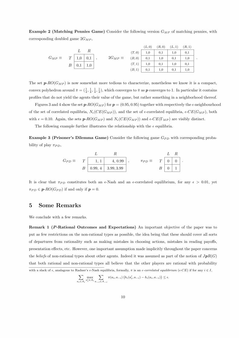
Example 2 (Matching Pennies Game) Consider the following version GMP of matching pennies, with

corresponding doubled game 2GMP ,

GMP ≡L R

T 1,0 0,1

B 0,1 1,0

, 2GMP ≡

(L, 0) (R, 0) (L, 1) (R, 1)

(T, 0) 1,0 0,1 1,0 0,1

(B, 0) 0,1 1,0 0,1 1,0

(T, 1) 1,0 0,1 1,0 0,1

(B, 1) 0,1 1,0 0,1 1,0

.

The set p-RO(GMP ) is now somewhat more tedious to characterize, nonetheless we know it is a compact,

convex polyhedron around π = ( 14 ,

14 ,

14 ,

14 ), which converges to π as p converges to 1. In particular it contains

profiles that do not yield the agents their value of the game, but rather something in a neighborhood thereof.

Figures 3 and 4 show the set p-RO(GMP ) for p = (0.95, 0.95) together with respectively the ε-neighbourhood

of the set of correlated equilibria, Nε(CE(GMP )), and the set of ε-correlated equilibria, ε-CE(GMP ), both

with ε = 0.10. Again, the sets p-RO(GMP ) and Nε(CE(GMP )) and ε-CE(ΓMP ) are visibly distinct.

The following example further illustrates the relationship with the ε equilibria.

Example 3 (Prisoner’s Dilemma Game) Consider the following game GPD with corresponding proba-

bility of play πPD,

GPD ≡L R

T 1, 1 4, 0.99

B 0.99, 4 3.99, 3.99

, πPD ≡L R

T 0 0

B 0 1

.

It is clear that πPD constitutes both an ε-Nash and an ε-correlated equilibrium, for any ε > 0.01, yet

πPD ∈ p-RO(GPD) if and only if p = 0.

5 Some Remarks

We conclude with a few remarks.

Remark 1 (P -Rational Outcomes and Expectations) An important objective of the paper was to

put as few restrictions on the non-rational types as possible, the idea being that these should cover all sorts

of departures from rationality such as making mistakes in choosing actions, mistakes in reading payoffs,

presentation effects, etc. However, one important assumption made implicitly throughout the paper concerns

the beliefs of non-rational types about other agents. Indeed it was assumed as part of the notion of JpR(G)

that both rational and non-rational types all believe that the other players are rational with probability

with a slack of ε, analagous to Radner’s ε-Nash equilibria, formally, π is an ε-correlated equilibrium (ε-CE) if for any i ∈ I,∑ai∈Ai

maxa′i∈Ai

∑a−i∈A−i

π(ai, a−i)(hi(a

′i, a−i)− hi(ai, a−i)

)≤ ε.

10

Figure 3: 0.95-RO(GMP ) (blue), N0.10CE(GMP ) (green)

Figure 4: 0.95-RO(GMP ) (blue), 0.10-CE(GMP ) (green)

11

pi or more. Another benchmark in line with our motivation would be to drop any restriction on the non-

rational types and allow them to have any kind of beliefs about others. This can be formalized by assuming

a larger vector P = (p,0) ∈ [0, 1]2I where the components associated to the rational types are the usual

probabilities p, while the components associated to the non-rational types are all zero. This leads to P -

rational outcomes of G. These are projections of (A× {0},P )-correlated equilibria of 2G, in that they are

distributions satisfying the same conditions as the (A× {0},p)-CE(2G) except that the p-belief constraints

for the non-rational types are dropped. In other words, (A× {0},p)-CE(2G) ⊂ (A× {0},P )-CE(2G) and

therefore also p-RO(G) ⊂ P -RO(G).

While the correspondence P -RO(G) maintains the basic topological properties of the correspondence

p-RO(G), it need not converge to the set of correlated equilibria of G as P → (1,0), but does so if one also

requires P → (1,1). This can be seen already in Example 1. A (1,0)-rational belief system can be very

far from a (1,1)-rational belief system in that the former need not put any restriction on the total mass of

rational types f(R).7

The alternative notion of approximate knowledge of rationality requiring f(CBp) > 1 − ε, for ε > 0,

(instead of JpB(R)), is more flexible with respect to the players’ beliefs in that it only restricts the total

mass of common p-belief and hence does not specify directly what beliefs individual players and types have.

A characterization of p-rational outcomes with this definition is possible along the lines of our Theorem 1,

but involves more complicated incentive and p-belief constraints that are imposed over all possible subsets

and permutations of players.

Remark 2 (Non-Common Priors) Throughout the paper we assumed the existence of a common prior

(CP ). This together with the notion of joint p-belief of rationality allowed us to derive relatively stringent

restrictions on behavior. At the same time it is natural to ask, what happens if the common prior assumption

is relaxed. As it turns out, under subjective or non-common priors, joint p-belief of rationality puts no

restrictions on possible behavior – even when p = 1. This provides a stark contrast with the cases of common

knowledge of rationality and also common p-belief of rationality as studied respectively in [2, 5, 7, 15, 17]

and [6, 12], and in a sense further highlights the stringency of the common prior assumption.8

To see the non-common prior case, define belief system B =⟨(Ti)i∈I , (si)i∈I , (fi)i∈I

⟩to be subjectively

p-rational if T =⋂i∈I B

pii (R−i). Given a finite game in strategic form G with set of players I and set

of action profiles A, and given p ∈ [0, 1]I , we say that a family of distributions (πi)i∈I ∈ (∆ (A))I

is a

7To see this, let P = (p, q) ∈ [0, 1]2I , where p, q are the probabilities for the rational and non-rational types respectively.To see that in a (1,0)-rational belief system the total mass of non-rational types is unrestricted, take the game in Example 1and consider the belief system B =

⟨(Ti)i∈I , (si)i∈I , (fi)i∈I

⟩, where Ti = Ai, si(ai) = ai, for all ai ∈ Ai, i ∈ I, and where

f ∈ ∆(A) is given by fTL = fTR = fBL = 0 and fBR = 1. It can be checked that it is (1,0)-rational and clearly f(R) = 0. Atthe same time, in a (p, q)-rational belief system it is always the case that, for any i ∈ I, ti ∈ Ti, fi(ti)(R−i) ≥ qi, hence

f(R−i ∩ (T−i × {ti}) ≥ qif(T−i × {ti}) =⇒∑

ti∈Ti

f(R−i ∩ (T−i × {ti}) = qi∑

ti∈Ti

f(T−i × {ti}) =⇒ f(R−i) ≥ qi,

which besides confirming the expected convergence to the correlated equilibria as (p, q)→ (1,1), also shows that positive qi’sdo put restrictions on the total mass of rational types f(R).

8Recall that the result of Lemma 1(a) also holds with non-common priors.

12

p-subjectively rational outcome of G (p-SRO(G)) if there exists some subjectively p-rational belief system

B =⟨(Ti)i∈I , (si)i∈I , (fi)i∈I

⟩for G such that for any i ∈ I, we have πi = fi ◦ [s]−1. As shown in the

Appendix, it is easy to see that, for any p ∈ [0, 1]I , the whole space is obtained, namely:

p-SRO (G) = (∆ (A))I.

In particular any pure strategy profile in A is consistent with subjective p-rationality, even when p = 1.

Remark 3 (Comparison with Further Solution Concepts) The sets of p-rational outcomes define sets

of probability distributions of play that are broader than the correlated equilibria that follow their own logic.

As the examples show, they are distinct from ε-neighbourhoods of the correlated equilibria, thus putting

further structure on the types of deviations from the set CE(G) that occur as p departs from 1. At the same

time, they are distinct from the ε-correlated equilibria, reflecting the fact that they impose no constraints

on the type of departure from rationality assumed – unlike with the ε-correlated equilibria, which assume

the agents are ε-optimizers. A similar remark applies to the quantal response equilibria of McKelvey and

Palfrey [13] or other models such as the level-k reasoning models (e.g, [8]) that put specific restrictions on

how players can deviate from rationality. It remains an empirical question to what extent the p-rational

outcomes bound observed behavior in a robust and useful manner.

Remark 4 (Learning to Play p-Rational Outcomes) Clearly, all learning dynamics that lead to corre-

lated equilibria (see e.g., [11]) will also lead to p-rational outcomes. The question arises as to what further

dynamics (not necessarily converging to correlated equilibria) may converge to p-rational outcomes and

whether they include interesting dynamics that for example allow for faster or more robust convergence.

References

[1] Aliprantis, C.D. and K.C. Border (2006) Infinite Dimensional Analysis: A Hitchhiker’s Guide, (Third

Ed.), Berlin, Springer Verlag.

[2] Aumann, R.J. (1974) “Subjectivity and Correlation in Randomized Strategies,” Journal of Mathematical

Economics, 1: 67–96.

[3] Aumann, R.J. (1987) “Correlated Equilibrium as an Expression of Bayesian Rationality,” Econometrica,

55: 1–18.

[4] Aumann, R.J. and J.H. Dreze (2008) “Rational Expectations in Games,” American Economic Review,

98: 72–86.

[5] Pearce, D. (1984) “Rationalizable Strategic Behavior,” Econometrica, 52: 1007–1028.

13

[6] Borgers, T. (1996) “Weak Dominance and Approximate Common Knowledge,” Journal of Economic

Theory, 64: 265-276.

[7] Brandenburger, A., and E. Dekel (1987) “Rationalizability and Correlated Equilibria,” Econometrica,

55: 1391–1402.

[8] Camerer, C.F. (2003) Behavioral Game Theory: Experiments in Strategic Interaction, New York, Prince-

ton University Press.

[9] Conlisk, J. (1996) “Why Bounded Rationality?,” Journal of Economic Literature, 34: 669-700.

[10] Harsanyi, J.C. (1967–1968) “Games with Incomplete Information Played by ‘Bayesian’ Players. I–III,”

Management Science, 14: 159–182, 320–334, 486–502.

[11] Hart, S. (2005) “Adaptive Heuristics,” Econometrica, 73: 1401–1430.

[12] Hu, T.W. (2007) “On p-Rationalizability and Approximate Common Certainty of Rationality,” Journal

of Economic Theory, 136: 379-391.

[13] McKelvey, R.D., and T.R. Palfrey (1995) “Quantal Response Equilibria in Normal Form Games,” Games

and Economic Behavior, 7: 6–38.

[14] Monderer, D. and D. Samet (1989) “Approximating Common Knowledge with Common Beliefs,” Games

and Economic Behavior, 1: 170–190.

[15] Pearce, D. (1994) “Rationalizable Strategic Behavior and the Problem of Perfection,” Econometrica,

52: 1029–1050.

[16] Rubinstein, A. (1998) Modelling Bounded Rationality, Cambridge, MA, MIT Press.

[17] Tan, T.C., and S.R. Werlang (1988) “The Bayesian Foundation of Solution Concepts of Games,” Journal

of Economic Theory, 45: 370-391.

14

APPENDIX

A Proofs of Lemma 1

(a) By definition, CBp (R) ⊆⋂i∈I B

pii (R), and therefore, for any i ∈ I, CBp (R) ⊆ Bpii (Ri). But now:

(t−i; ti) ∈ Bpii (Ri) ⇐⇒ fi (ti) (Ri) =f (Ri ∩ (T−i × {ti}))

f (T−i × {ti})≥ pi.

So, as pi > 0, T−i × {ti} ⊆ Ri and therefore, Bpii (Ri) ⊆ Ri.

(b) First, if T =⋂i∈I B

pi (R−i), then:

R = R ∩ T =⋂i∈I

(Bpi (R−i) ∩Ri) =⋂i∈I

Bpii (R) ⊆ CBp (R) ,

and therefore, R ⊆ CBp (R). Now, again, since T =⋂i∈I B

pi (R−i), we have both:

f (R−i) ≥ p, and f (R−i ∩Ri) ≥ pf (Ri) .

The fact that, for any j 6= i, f (R) = f (R−i|Ri) f (Ri) ≥ pf (Ri) ≥ pf (R−j) ≥ p2 completes the proof.

(c) As mentioned in the paper, it is easy to check that:

T = (CBp)|p=1 (R) ⇐⇒ T =⋂i∈I

B1i (R) .

Now, take t = (ti)i∈I . Then,

t ∈⋂i∈I

B1i (R) ⇐⇒ ∀i ∈ I, fi(ti)(R) = 1 ⇐⇒

⇐⇒ ∀i ∈ I, fi (R ∩ (T−i × {ti})) = fi (T−i × {ti})∗⇐⇒

∗⇐⇒ ∀i ∈ I, fi (R−i ∩ (T−i × {ti})) = fi (T−i × {ti}) ⇐⇒

⇐⇒ t ∈⋂i∈I

B1i (R−i) .

* The left implication is immediate; the right implication is a consequence of the non-emptiness of

R ∩ (T−i × {ti}).

15

B Proof of Theorem 1

We first introduce and prove the following lemma:

Lemma 2 Let G a finite game in strategic form, p ∈ [0, 1]I, n ∈ N, k ≤ n, and π ∈ (A× {k} ,p) -CE (nG).

Let, B =⟨(nAi)i∈I , (si)i∈I , π

⟩where si (ai, αi) = ai for any (ai, αi) ∈ nAi, and any i ∈ I. B is a p-rational

belief system for G such that πB = ProjA (π).

Proof. Since π is a (A× {k} ,p)-correlated equilibrium of nG:

• From the incentive constraints we know that for any i ∈ I, Ai × {k} ⊆ Ri.

• From the p-belief constraints we know that for any i ∈ I, and any (ai, αi) ∈ nAi:

π ((A−i × {k−i})× {(a, αi)}) ≥ piπ (nA−i × {(ai, αi)}) .

Thus, we obtain that for any (ai, αi) ∈ nAi, π (R−i ∩ (nA−i × {(ai, αi)})) ≥ piπ (nAi × {(ai, αi)}),

and therefore, that B is p-rational.

Finally, πB = ProjA (π) is an obvious identity.

Let’s go on with the proof of the theorem. For k ∈ {0, 1}; by −k we denote the element complementary

to k in this set.

⊆

Let B =⟨(Ti)i∈I , (si)i∈I , f

⟩a p-rational belief system for G. For each player i ∈ I we can define:

βk,i : Ti −→ 2Ai

ti ∈ Ri → (si (i) , k)

ti /∈ Ri → (si (i) ,−k)

Now, for any (a, α) ∈ 2A, let π (a, α) = f(∏

i∈I β−1k,i (ai, αi)

). It is immediate that ProjA (π) = πB . Let’s

check that π is a (A× {k} ,p)-correlated equilibrium of 2G. Let i ∈ I:

• Let (ai, k) ∈ Ai × {k} and (ai, αi) ∈ 2Ai. Then:

∑(a−i,αi)∈2A−i

π ((a−i, α−i) ; (ai, k))h2,i ((a−i, α−i) ; (a, αi)) =

=∑

ti∈[βk,i]−1(ai,k)

f(T−i × {ti} |[βk,i]−1 (ai, k)

) ∑a−i∈A−i

EB [hi (a−i; ai) |fi (ti)] .

Since by construction, T−i × [βk,i]−1 (ai, k) ⊆ Ri, (ai, k) is maximizer of the above.

16

• Let (ai, αi) ∈ 2Ai. Then:

π ((A−i × {k−i})× {ai, αi}) =

= f(R−i ∩

(T−i × [βk,i]

−1 (ai, αi)))≥ pif

(T−i × [βk,i]

−1 (ai, αi))

= piπ (2A−i × {(ai, αi)}) .

⊇

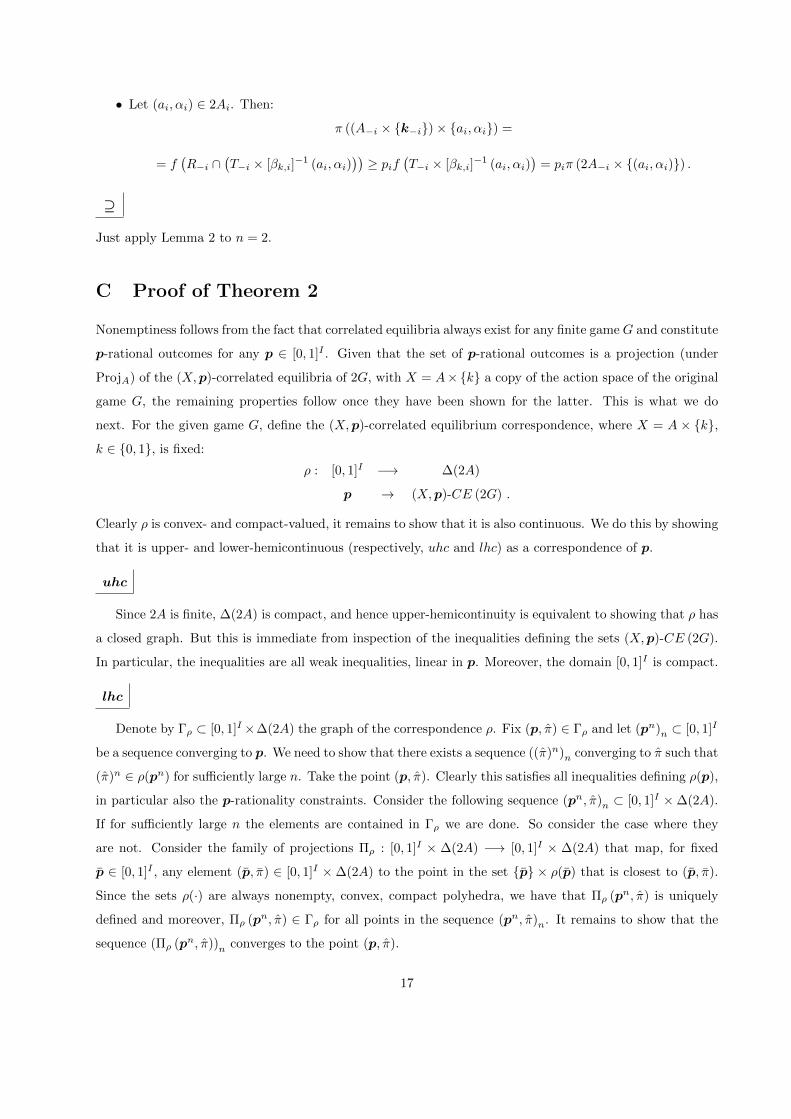
Just apply Lemma 2 to n = 2.

C Proof of Theorem 2

Nonemptiness follows from the fact that correlated equilibria always exist for any finite game G and constitute

p-rational outcomes for any p ∈ [0, 1]I . Given that the set of p-rational outcomes is a projection (under

ProjA) of the (X,p)-correlated equilibria of 2G, with X = A×{k} a copy of the action space of the original

game G, the remaining properties follow once they have been shown for the latter. This is what we do

next. For the given game G, define the (X,p)-correlated equilibrium correspondence, where X = A × {k},

k ∈ {0, 1}, is fixed:

ρ : [0, 1]I −→ ∆(2A)

p → (X,p)-CE (2G) .

Clearly ρ is convex- and compact-valued, it remains to show that it is also continuous. We do this by showing

that it is upper- and lower-hemicontinuous (respectively, uhc and lhc) as a correspondence of p.

uhc

Since 2A is finite, ∆(2A) is compact, and hence upper-hemicontinuity is equivalent to showing that ρ has

a closed graph. But this is immediate from inspection of the inequalities defining the sets (X,p)-CE (2G).

In particular, the inequalities are all weak inequalities, linear in p. Moreover, the domain [0, 1]I is compact.

lhc

Denote by Γρ ⊂ [0, 1]I×∆(2A) the graph of the correspondence ρ. Fix (p, π) ∈ Γρ and let (pn)n ⊂ [0, 1]I

be a sequence converging to p. We need to show that there exists a sequence ((π)n)n converging to π such that

(π)n ∈ ρ(pn) for sufficiently large n. Take the point (p, π). Clearly this satisfies all inequalities defining ρ(p),

in particular also the p-rationality constraints. Consider the following sequence (pn, π)n ⊂ [0, 1]I ×∆(2A).

If for sufficiently large n the elements are contained in Γρ we are done. So consider the case where they

are not. Consider the family of projections Πρ : [0, 1]I × ∆(2A) −→ [0, 1]I × ∆(2A) that map, for fixed

p ∈ [0, 1]I , any element (p, π) ∈ [0, 1]I ×∆(2A) to the point in the set {p} × ρ(p) that is closest to (p, π).

Since the sets ρ(·) are always nonempty, convex, compact polyhedra, we have that Πρ (pn, π) is uniquely

defined and moreover, Πρ (pn, π) ∈ Γρ for all points in the sequence (pn, π)n. It remains to show that the

sequence (Πρ (pn, π))n converges to the point (p, π).

17

Apart from the p-belief constraints all other constraints defining ρ(p) are independent of p. Hence,

if (p, π) satisfies those constraints, then so must any other point in the sequence (pn, π)n. Therefore the

only constraints that can be violated by elements of the sequence (pn, π)n are the p-belief constraints.

Consequently, any point in the sequence (Πρ (pn, π))n lies on the boundary of the polyhedra defined by the

p-belief constraints. As mentioned, these constraints are linear in p, and since they also define nonempty,

convex, compact polyhedra, the sequence (Πρ (pn, π))n indeed converges to (p, π). This shows the continuity

of ρ and hence also of p-RO(G) in p.

Finally, the claims that, for p = 0, we have 0-RO(G) = ∆(A), and for p = 1, we have 1-RO(G) = CE(G),

are immediate. To see that for any p ∈ [0, 1), we have dim[p-RO(G)] = dim[∆(A)], notice that the (X,p)-

correlated equilibria with X = A1 and p < 1 entail distributions that put strictly positive weight on all

strategies in A2 as well as all convex combinations of such distributions. Projecting onto the original space

∆(A) implies distributions with strictly positive weights on all strategies in A as well as all possible convex

combinations. This concludes the proof.

D Proof of Proposition 1

Fix G and let An = Πi∈IAni denote the space of all pure strategy profiles that survive n rounds of iterated

elimination of strictly dominated strategies in G, and similarly for the individual sets Ani . Let Gn denote

the subgame of G with strategies restricted to An. Because G is finite, the limit sets A∞i , A∞, and G∞ are

well defined (and are obtained after finitely many iterations). Also, for any subset Y ⊂ A, let Y c = A \ Y

denote the complement of Y in A.

For any given p ∈ [0, 1], let p ∈ [0, 1]I

be such that min p ≥ p. We show that for p sufficiently close to 1,

behavior is supported with high probability (p) in A∞. Specifically, we construct a p < 1 such that for any

p ∈ [p, 1], if π ∈ p-RO(G), then π ((A∞)c) ≤ 1− p.

Consider the game G0 = G and pick some p1 < 1. It immediately follows from p-rationality that for

p ∈ [p1, 1], if π ∈ p-RO(G), we have π((A1)c) ≤ 1− p.

Suppose now that the above statement is true for n − 1, namely there exists pn−1 < 1 such that for

p ∈ [pn−1, 1], if π ∈ p-RO(G), then we have π((An−1

)c) ≤ 1 − p. We show that the statement also holds

for n.

Fix the game Gn−1. It follows from finiteness of G and continuity of the payoffs that there exists

pn ∈ [pn−1, 1) such a strategy in An−1 \ An that is strictly dominated in Gn−1 (by some strategy in Gn−1

and hence in G) is also strictly dominated in G (by the same strategy) given a p-rational belief system

with minp ≥ p and p ≥ pn; (this follows from pn ≥ pn−1, and because π ∈ p-RO(G) with p ≥ pn−1

implies π((An−1

)c) ≤ 1 − p). This implies that for any p ∈ [pn, 1] and any π ∈ p-RO(G), we also have

π ((An)c) ≤ 1− p.

Finiteness of the game implies that the process ends after finitely many steps implying that indeed there

18

exists p∞ < 1 such that for p ∈ [p∞, 1] and any π ∈ p-RO(G), we have π ((A∞)c) ≤ 1 − p. Taking p = p∞

shows the claim.

E Proof of Theorem 3

We prove the first statement. The one concerning the p-rational expectation of rational types becomes

obvious after that proof. The statement is given for k = 0, and we suppose we are taking some player i0’s

expectation.

⊆

Let B =⟨(Ti)i∈I , (si)i∈I , f

⟩a p-rational belief system for G, i0 ∈ I, and ti0 ∈ Ti0 . For any i ∈ I \ {i0}, we

define:

βk,i : Ti −→ 3Ai

ti ∈ Ri → (si (ti) , k)

ti /∈ Ri → (si (ti) , k + 1 mod 3)

and:

βk,i0 : Ti −→ 3Ai0

t′i0 ∈ Ri0 \ {ti0} → (si0 (ti0) , k)

t′i0 /∈ Ri0 ∪ {ti0} → (si0 (ti0) , k + 1 mod 3)

t′i0 = ti0 → (si0 (ti0) , k + 2 mod 3)

By an identical argument to the one in the first part of the proof of Theorem 1, we can conclude that π =

f ◦β−1 is a (A× {k} ,p)-correlated equilibrium of G, and it is immediate that EB [hi0 (a−i0 ; si0 (ti0)) |fi0 (ti0)]

is exactly player i0’s expectation conditional on playing (si0 (ti0) , k + 2 mod 3) induced by π.

⊇

It is again a reduction of Lemma 2, this time to n = 3.

F Proof of Result in Remark 2

Following Aumann, [2, 3], for any X =∏i∈I Xi ⊆ A, we say that the family (πi)i∈I ⊆ (∆ (A))

Iis a

(X,p)-subjective correlated equilibrium of G, if for any i ∈ I:

• For any a′i ∈ Xi, the following incentive constraints are satisfied:

∑a−i∈A−i

πi (a−i; a′i) [hi (a−i; a

′i)− hi (a−i; ai)] ≥ 0, for any ai ∈ Ai,

19

• For any ai ∈ Ai the following pi-belief constraint is satisfied:

∑a′−i∈X−i

πi(a′−i; ai

)≥ pi

∑a−i∈A−i

πi (a−i; ai) .

We denote the set of (X,p)-subjective correlated equilibria of game G by (X,p) -SCE (G). Given n ∈ N and

a n-game nG, we have the projection ProjAI : (∆ (nA))I → (∆ (A))

I, where for any (πi)i∈I ∈ (∆ (nA))

I,

ProjAI

((πi)i∈I

)= (ProjA (πi))i∈I . Then, the proof of the identity:

p-SRO (G) = ProjAI [(A× {0}) -SCE (2G)]

is the same as the one for Theorem 1 after slight modifications (just add sub-indices where needed). To

see that the above projections constitute the whole space, let(ai)i∈I ⊆ A, and for any i ∈ I, πi = 1{ai}.

Fix k ∈ {0, 1}, and define, for any i ∈ I, πi = 1{((ai−i,k−i);(aii,−k))}. It is immediate that ProjA((πi)i∈I

)=

(πi)i∈I . Now, let i ∈ I, then the incentive constraints are trivially satisfied, since πi (2A−i × (Ai × {k})) = 0.

Moreover, the pi-belief constraint is also satisfied, because regardless of i’s action, the sums are on both sides

1 or 0. We conclude that(1{ai}

)i∈I ∈ ProjA ((A× {k} ,p) -SCE (2G)) for any

(ai)i∈I ⊆ A, so by convexity,

ProjA ((A× {k} ,p) -SCE (2G)) = (∆ (A))I.

20