approximate neural networks for speech … neural networks for speech applications in...
TRANSCRIPT

Approximate Neural Networks for Speech Applications in
Resource-Constrained Environments
by
Sairam Arunachalam
A Thesis Presented in Partial Fulfillmentof the Requirements for the Degree
Master of Science
Approved May 2016 by theGraduate Supervisory Committee:
Chaitali Chakrabarti, Co-ChairJae-sun Seo, Co-Chair
Yu Cao
ARIZONA STATE UNIVERSITY
August 2016
ABSTRACT
Speech recognition and keyword detection are becoming increasingly popular appli-
cations for mobile systems. While deep neural network (DNN) implementation of
these systems have very good performance, they have large memory and compute
resource requirements, making their implementation on a mobile device quite chal-
lenging. In this thesis, techniques to reduce the memory and computation cost of
keyword detection and speech recognition networks (or DNNs) are presented.
The first technique is based on representing all weights and biases by a small num-
ber of bits and mapping all nodal computations into fixed-point ones with minimal
degradation in the accuracy. Experiments conducted on the Resource Management
(RM) database show that for the keyword detection neural network, representing the
weights by 5 bits results in a 6 fold reduction in memory compared to a floating point
implementation with very little loss in performance. Similarly, for the speech recogni-
tion neural network, representing the weights by 6 bits results in a 5 fold reduction in
memory while maintaining an error rate similar to a floating point implementation.
Additional reduction in memory is achieved by a technique called weight pruning,
where the weights are classified as sensitive and insensitive and the sensitive weights
are represented with higher precision. A combination of these two techniques helps re-
duce the memory footprint by 81 - 84% for speech recognition and keyword detection
networks respectively.
Further reduction in memory size is achieved by judiciously dropping connec-
tions for large blocks of weights. The corresponding technique, termed coarse-grain
sparsification, introduces hardware-aware sparsity during DNN training, which leads
to efficient weight memory compression and significant reduction in the number of
computations during classification without loss of accuracy. Keyword detection and
speech recognition DNNs trained with 75% of the weights dropped and classified with
i

5-6 bit weight precision effectively reduced the weight memory requirement by ∼95%
compared to a fully-connected network with double precision, while showing similar
performance in keyword detection accuracy and word error rate.
ii

DEDICATION
To my family for their support
iii

ACKNOWLEDGEMENTS
I would like to express my sincere gratitude to Dr. Chaitali Charkrabarti and Dr.
Jae-sun Seo for their continuous guidance throughout my research work during the
past year. I’m also grateful to Dr. Yu Cao for taking the time to review my work.
I would like to thank Dr. Mohit Shah for his support throughout my research
work. He introduced me to speech recognition tools and helped me even after his
graduation. I’m grateful to Deepak Kadetotad for his insights into my research and
collaboration in the project.
I also thank my parents, brother, friends and roommates for supporting me though
the past two years.
I also gratefully acknowledge the financial support provided by Dr. Jae-sun Seo
and Dr. Chaitali Chakrabarti.
iv
TABLE OF CONTENTS
Page
LIST OF TABLES . . . . . . . . . . . . . . . . . . . . . . . . . . . . . . . . . . . . . . . . . . . . . . . . . . . . . . . . . vii
LIST OF FIGURES . . . . . . . . . . . . . . . . . . . . . . . . . . . . . . . . . . . . . . . . . . . . . . . . . . . . . . . . viii
CHAPTER
1 INTRODUCTION . . . . . . . . . . . . . . . . . . . . . . . . . . . . . . . . . . . . . . . . . . . . . . . . . . . 1
1.1 Speech Recognition, Keyword Detection . . . . . . . . . . . . . . . . . . . . . . . . . . 1
1.2 Speech Recognition and Keyword Detection with Neural Networks . 2
1.3 Problem Definition. . . . . . . . . . . . . . . . . . . . . . . . . . . . . . . . . . . . . . . . . . . . . . 3
1.4 Proposed Method . . . . . . . . . . . . . . . . . . . . . . . . . . . . . . . . . . . . . . . . . . . . . . . 4
1.5 Contributions . . . . . . . . . . . . . . . . . . . . . . . . . . . . . . . . . . . . . . . . . . . . . . . . . . 4
1.6 Organization . . . . . . . . . . . . . . . . . . . . . . . . . . . . . . . . . . . . . . . . . . . . . . . . . . . 5
2 BACKGROUND . . . . . . . . . . . . . . . . . . . . . . . . . . . . . . . . . . . . . . . . . . . . . . . . . . . . 6
2.1 Deep Neural Network Structure . . . . . . . . . . . . . . . . . . . . . . . . . . . . . . . . . . 6
2.2 Training Strategy for DNNs . . . . . . . . . . . . . . . . . . . . . . . . . . . . . . . . . . . . . 8
2.3 Keyword Detection . . . . . . . . . . . . . . . . . . . . . . . . . . . . . . . . . . . . . . . . . . . . . 10
2.3.1 Input Features . . . . . . . . . . . . . . . . . . . . . . . . . . . . . . . . . . . . . . . . . . . 10
2.3.2 Data Preparation . . . . . . . . . . . . . . . . . . . . . . . . . . . . . . . . . . . . . . . . 10
2.3.3 Neural Network Architecture . . . . . . . . . . . . . . . . . . . . . . . . . . . . . 11
2.3.4 Post Processing . . . . . . . . . . . . . . . . . . . . . . . . . . . . . . . . . . . . . . . . . . 11
2.3.5 Evaluation . . . . . . . . . . . . . . . . . . . . . . . . . . . . . . . . . . . . . . . . . . . . . . 12
2.4 Speech Recognition . . . . . . . . . . . . . . . . . . . . . . . . . . . . . . . . . . . . . . . . . . . . . 13
2.4.1 Input Features . . . . . . . . . . . . . . . . . . . . . . . . . . . . . . . . . . . . . . . . . . . 13
2.4.2 Neural Network Architecture . . . . . . . . . . . . . . . . . . . . . . . . . . . . . 13
2.4.3 Post Processing . . . . . . . . . . . . . . . . . . . . . . . . . . . . . . . . . . . . . . . . . . 14
2.4.4 Evaluation . . . . . . . . . . . . . . . . . . . . . . . . . . . . . . . . . . . . . . . . . . . . . . 15
v
CHAPTER Page
2.5 Simulation Setup . . . . . . . . . . . . . . . . . . . . . . . . . . . . . . . . . . . . . . . . . . . . . . . 15
3 FIXED POINT ARCHITECTURE AND WEIGHT PRUNING . . . . . . . . . 17
3.1 Fixed-Point NN for Keyword Detection . . . . . . . . . . . . . . . . . . . . . . . . . . . 17
3.2 Fixed-Point NN for for Speech Recognition . . . . . . . . . . . . . . . . . . . . . . . 20
3.3 Weight Pruning. . . . . . . . . . . . . . . . . . . . . . . . . . . . . . . . . . . . . . . . . . . . . . . . . 22
3.3.1 Results . . . . . . . . . . . . . . . . . . . . . . . . . . . . . . . . . . . . . . . . . . . . . . . . . . 23
3.4 Conclusions . . . . . . . . . . . . . . . . . . . . . . . . . . . . . . . . . . . . . . . . . . . . . . . . . . . . 25
4 COARSE GRAIN SPARSIFICATION . . . . . . . . . . . . . . . . . . . . . . . . . . . . . . . . 26
4.1 Overview. . . . . . . . . . . . . . . . . . . . . . . . . . . . . . . . . . . . . . . . . . . . . . . . . . . . . . . 26
4.2 Block Structure . . . . . . . . . . . . . . . . . . . . . . . . . . . . . . . . . . . . . . . . . . . . . . . . . 27
4.3 Training of Sparse Neural Networks . . . . . . . . . . . . . . . . . . . . . . . . . . . . . . 28
4.4 Results . . . . . . . . . . . . . . . . . . . . . . . . . . . . . . . . . . . . . . . . . . . . . . . . . . . . . . . . 29
4.4.1 Keyword Detection. . . . . . . . . . . . . . . . . . . . . . . . . . . . . . . . . . . . . . . 29
4.4.2 Speech Recognition . . . . . . . . . . . . . . . . . . . . . . . . . . . . . . . . . . . . . . 33
4.5 Conclusions . . . . . . . . . . . . . . . . . . . . . . . . . . . . . . . . . . . . . . . . . . . . . . . . . . . . 36
5 CONCLUSIONS. . . . . . . . . . . . . . . . . . . . . . . . . . . . . . . . . . . . . . . . . . . . . . . . . . . . . 37
5.1 Summary . . . . . . . . . . . . . . . . . . . . . . . . . . . . . . . . . . . . . . . . . . . . . . . . . . . . . . 37
5.2 Future Work . . . . . . . . . . . . . . . . . . . . . . . . . . . . . . . . . . . . . . . . . . . . . . . . . . . 38
REFERENCES . . . . . . . . . . . . . . . . . . . . . . . . . . . . . . . . . . . . . . . . . . . . . . . . . . . . . . . . . . . . 39
vi
LIST OF TABLES
Table Page
3.1 AUC and Memory Requirements of Floating and Fixed Point Imple-
mentations for Keyword Detection Network . . . . . . . . . . . . . . . . . . . . . . . . . . 20
3.2 WER and Memory Requirements of Floating and Fixed-Point Imple-
mentations for Speech Recognition Network. . . . . . . . . . . . . . . . . . . . . . . . . . 22
3.3 Memory Requirement of Networks with Pruned Weights . . . . . . . . . . . . . . 24
4.1 AUC and Memory Requirements of Floating and Fixed Point Imple-
mentations for Keyword Detection Network . . . . . . . . . . . . . . . . . . . . . . . . . . 31
4.2 WER and Memory Requirements of Floating and Fixed-Point Imple-
mentations for Speech Recognition Network. . . . . . . . . . . . . . . . . . . . . . . . . . 36
vii

LIST OF FIGURES
Figure Page
2.1 A Feed-Forward Neural Network with a Single Hidden Layer . . . . . . . . . . 7
2.2 A Model of a Neuron with ReLU Activation In a Feed-Forward Neural
Network Architecture . . . . . . . . . . . . . . . . . . . . . . . . . . . . . . . . . . . . . . . . . . . . . . 8
2.3 Neural Network Architecture for Keyword Detection Consists of 2 Hid-
den Layers with 512 Neurons Per Layer. The Input Feature Dimension
Is 403 and the Output Dimension Is 12 (10 Keywords, 1 OOV and 1
Silence) . . . . . . . . . . . . . . . . . . . . . . . . . . . . . . . . . . . . . . . . . . . . . . . . . . . . . . . . . . . 12
2.4 Neural Network Architecture for the Speech Recognition System Con-
sists of Four Hidden Layers with 1024 Neurons Per Layer. The Input
Feature Dimension Is 440 and the Output Layer Consists of 1483 Nodes
Representing the Posterior Probability of the 1483 HMM States . . . . . . . 14
3.1 A Comparison of the Average ROC Across All Keywords Between Net-
works with Different Number of Nodes Per Hidden Layer . . . . . . . . . . . . . 18
3.2 Histogram of Weights and Biases for Keyword Detection Neural Network 19
3.3 Effect of Fractional Precision of Weights and Biases On the Average
AUC for Keyword Detection Network . . . . . . . . . . . . . . . . . . . . . . . . . . . . . . . 19
3.4 Histogram of Weights for Speech Recognition Neural Network . . . . . . . . . 21
3.5 Effect of Fractional Precision of Weights On WER for Speech Recog-
nition Network . . . . . . . . . . . . . . . . . . . . . . . . . . . . . . . . . . . . . . . . . . . . . . . . . . . . 22
3.6 Effect of Threshold On AUC for Keyword Detection Neural Network . . 24
3.7 Effect of Weight Pruning Threshold On WER for Speech Recognition
Network . . . . . . . . . . . . . . . . . . . . . . . . . . . . . . . . . . . . . . . . . . . . . . . . . . . . . . . . . . . 25
4.1 Weight Matrix Compression . . . . . . . . . . . . . . . . . . . . . . . . . . . . . . . . . . . . . . . . 28
viii

Figure Page
4.2 Effect of Block Size and Percentage Dropout On WER of Speech Recog-
nition Network . . . . . . . . . . . . . . . . . . . . . . . . . . . . . . . . . . . . . . . . . . . . . . . . . . . . 30
4.3 Histogram of Weights and Biases of CGS Architecture with 64×64 At
75% Drop for Keyword Detection . . . . . . . . . . . . . . . . . . . . . . . . . . . . . . . . . . . 32
4.4 Effect of Fractional Precision of Weights and Bias On Average AUC of
Keyword Detection Network for CGS Architecture . . . . . . . . . . . . . . . . . . . 32
4.5 ROC Curve of Different Deep Neural Network Implementations for
Keyword Detection. . . . . . . . . . . . . . . . . . . . . . . . . . . . . . . . . . . . . . . . . . . . . . . . . 33
4.6 Effect of Block Size and Percentage Dropout On WER of Speech Recog-
nition Network . . . . . . . . . . . . . . . . . . . . . . . . . . . . . . . . . . . . . . . . . . . . . . . . . . . . 34
4.7 Histogram of Weights and Biases of CGS Architecture with 64×64 At
75% Drop . . . . . . . . . . . . . . . . . . . . . . . . . . . . . . . . . . . . . . . . . . . . . . . . . . . . . . . . . 35
4.8 Effect of Fractional Precision of Weights and Bias On WER of Speech
Recognition System for CGS Architecture . . . . . . . . . . . . . . . . . . . . . . . . . . . 35
ix
Chapter 1
INTRODUCTION
1.1 Speech Recognition, Keyword Detection
Automatic Speech Recognition (ASR) refers to the task of converting speech/audio
input to text. Applications for speech recognition include speech-to-text systems
(for word processors), personal assistance systems (Apple Siri, Google Now, Amazon
Alexa, etc.). Keyword detection refers to the task of detecting specific keywords
embedded in speech. Keyword detection can be used to control the front-end in
personal assistant systems to trigger a speech recognition engine, or in performing
certain actions depending on keyword detected in speech (e.g. “call home”).
A speech signal can be modeled as a stationary process in a short time scale
(frame) of 25ms. It can also be thought of as a Markov process where the probability
of the future outputs depends not only on the current state but also on the previous
states. This makes Hidden Markov Models (HMM) (Baker et al., 2009) an appropriate
choice to model acoustic information.
There is a vast amount of literature for both speech recognition and keyword
detection systems. For speech recognition, the usual process involves using a Hidden
Markov Model (HMM) for modeling the sequence of words/phonemes and using a
Gaussian Mixture Model (GMM) for acoustic modeling (Su et al., 2010; Sha and Saul,
2006; Juang et al., 1986; Gales and Young, 2008). This modeling can be done using
the Expectation-Maximization method. The most likely sequence can be determined
from the HMMs by employing the Viterbi algorithm. The GMMs can be implemented
in a parallel fashion, but the Viterbi algorithm is inherently sequential.
1
Keyword detection falls under speech recognition umbrella and is relatively less
complex. There are different approaches for detecting a keyword. For instance, the
speech recognition system can be used to perform keyword detection. In this ap-
proach, first speech recognition is performed and then keywords are detected from
the decoded transcription (Miller et al., 2007; Parlak and Saraclar, 2008; Mamou
et al., 2007). The drawback for such a method is that it requires the entire phrase to
be decoded before the keywords can be detected. The second method involves train-
ing separate models for keywords and out-of-vocabulary (OOV) words and detecting
keywords based on the likelihood over each model. A separate GMM-HMM is trained
for each keyword and the out-of-vocabulary words are modeled using a garbage or
filler model (Rohlicek et al., 1989; Rose and Paul, 1990; Wilpon et al., 1991; Silaghi
and Bourlard, 1999; Silaghi, 2005). Such a system is suitable in environments where
the set of keywords is known beforehand.
1.2 Speech Recognition and Keyword Detection with Neural Networks
Recently, neural network (NN) based methods have shown tremendous success
in speech recognition tasks. This success has come after advances made in the field
of deep learning (Dahl et al., 2011; Chen et al., 2014). These networks are well-
suited to capture the complex and non-linear patterns from the acoustic properties of
speech. Detection is performed through feed-forward computation; a matrix-vector
multiplication step followed by a non-linear operation at each layer, making it highly
suitable for parallel implementations. One such implementation for keyword detection
was presented in (Chen et al., 2014), for keyword detection. This system was also
shown to outperform the traditional GMM-HMM based approach. While its detection
performance was very good, the network was quite large, requiring up to a few million
multiplications every few milliseconds as well as large memory banks for storing the
2

weights.
The neural network for a typical speech recognition system is even larger and a
straightforward implementation would require huge memory for storing the weights
and large number of compute resources. The DNNs in speech recognition are used to
predict the probabilities of the different HMM states. Traditionally the GMMs were
used to model the relationship between the HMM states (Juang et al., 1986). The
GMMs failed to model data that lie on a non-linear manifold in dataspace. Artificial
neural networks, trained through backpropagation, have the potential to learn such
data representations (Hinton et al., 2012). In our work, the traditional GMM-HMM
model is used to derive the target vectors for training the DNN-HMM hybrid system.
The DNN based speech model is also shown to outperform the traditional GMM
based model (Dahl et al., 2012).
1.3 Problem Definition
The neural networks for speech recognition and keyword detection have large mem-
ory and compute resource requirements, making their implementation on a mobile
device quite challenging. Keyword detection engine can run as a background service
to an ASR in a mobile environment. Since it is always ‘on’, its power consumption has
to be very small. Compared to the keyword detection engine, the automatic speech
recognition system has very high memory and compute resource requirements. Im-
plementing such a system in a mobile or resource constrained environment is even
more challenging. Thus there is a strong need to develop an architectural frame-
work for such applications with the goal of reducing memory footprint and lowering
power consumption. In this thesis, low cost neural network architectures for keyword
detection and speech recognition have been designed and their performance analyzed.
3

1.4 Proposed Method
Reduction in memory and power of a neural network can be achieved in many
ways such as reducing the number of hidden layers, reducing size of hidden layers,
pruning the precision of weights and dropping weights and biases. Methods to reduce
the size of the hidden layer and scaling down the precision of the weights and biases
have been researched in (Shah et al., 2015). In order to further reduce the memory
requirement of the neural network, we propose two approaches. In the first method
called weight pruning (detailed in Chapter 3), the connections (weights and biases) are
classified as sensitive and insensitive based on the error produced by the connections
and the insensitive connections are scaled to a lower precision. In the second approach
(detailed in Chapter 4) we drop/remove a large portion of connections within a neural
network in a block structure to form a coarse-grain sparse weight matrix. The dropped
connections are not stored in the memory, which leads in a reduced memory footprint
for the network. The proposed systems are shown to perform at par with a fully
connected neural network with floating point architecture while requiring only a small
fraction of the memory.
1.5 Contributions
Overall, this thesis makes the following contributions.
� Design of fixed point neural network architecture with 4 hidden layers and 1024
neurons per layer for speech recognition. The weights and biases are represented
by 6 bits resulting in memory requirement reducing from 19.53MB to 3.66MB,
while maintaining a word error rate of 1.77%.
� Development of an algorithm to classify weights based on their sensitivity and
represent insensitive weights with lower precision to reduce memory require-
4

ment. This method was applied to speech recognition and keyword detection
networks resulting in 0.82 -2.12% memory reduction with loss in accuracy by
0.03 AUC and 0.17% reduction in WER, respectively.
� Development of static coarse-grain sparsification technique that can substan-
tially reduce the memory footprint as well as computations when deep neural
networks are implemented in hardware with minimal degradation in accuracy.
� A combination of fixed point implementation along with the coarse-grain drop-
connect structure reduced the memory requirement of the speech recognition
network from 19.53MB to 0.85MB with word error rate of 1.64%.
� A combination of fixed point implementation along with the coarse-grain drop-
connect structure reduced the memory requirement of the keyword detection
network from 1.81M to 101.26KB with detection accuracy of 0.91 AUC.
1.6 Organization
The reminder of the thesis is organized as follows. In Chapter 2, we discuss the
background details of DNN training and its application in speech recognition and
keyword detection. A method to prune the weights and biases based on their relative
sensitivity is discussed in Chapter 3. In Chapter 4, a coarse-grain sparsification
methodology to compress weight memory is described. Finally, the conclusions and
future work are presented in Chapter 5.
5
Chapter 2
BACKGROUND
2.1 Deep Neural Network Structure
A Deep Neural Network (DNN) is an artificial neural network with multiple hidden
layers between the input layer and output layer. A simple neural network consisting
of a single hidden layer is shown in Figure 2.1. DNNs have shown to be capable of
learning complex non-linear relationship present in data. In recent years, DNNs have
been implemented for image recognition and speech recognition tasks, significantly
outperforming their predecessors performance.
At a high level, a DNN consists of multiple layers of non-linear information pro-
cessing, where each layer is trained using supervised/unsupervised method (Deng
and Yu, 2014). One aspect of DNNs is to learn representation of data from examples.
DNNs attempt to learn feature representation of data from supervised learning algo-
rithms and these models can substitute the traditional handcrafted features used in
learning algorithms (Song and Lee, 2013).
In a feed-forward DNN, the neurons in one layer of the network are connected
to neurons in the next layer. The neurons within a layer are not connected and no
cycles are allowed within the network. There are certain architectures where cycles
in connections are allowed, but in this thesis we only consider feed-forward networks.
The computations involved in a neuron are described by Eqn. (2.1).
nj =N∑i=0
wij ∗ xi + bj (2.1)
where wij is the weight of the connection between ith neuron in the previous layer
6

Figure 2.1: A feed-forward neural network with a single hidden layer.
and the jth neuron in the current layer, bj is the bias value for the current neuron
and N is the number of input neurons.
The weighted sum is processed using a non-linear transformation to obtain the
output. While any non-linear function can be used to model the neuron output,
typically sigmoid (Eqn. (2.2)), ReLU (Eqn. (2.3)) or tanh are used. The ReLU
activation best mimics the biological neuron model and is commonly used in recent
deep networks.
h1j =
1
(1 + e−z1j )(2.2)
h1j = max(0, z1j ) (2.3)
The networks with ReLU activation are easier to train and no pre-training is gen-
erally required for such networks (Zeiler et al., 2013). Moreover, the ReLU activation
requires a simple comparison operation compared to sigmoid or tahn functions. This
makes the hardware implementation simple and reduces energy costs associated with
7
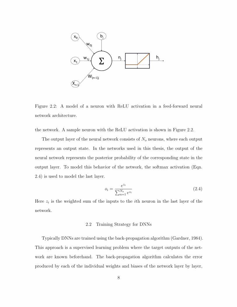
Figure 2.2: A model of a neuron with ReLU activation in a feed-forward neural
network architecture.
the network. A sample neuron with the ReLU activation is shown in Figure 2.2.
The output layer of the neural network consists of No neurons, where each output
represents an output state. In the networks used in this thesis, the output of the
neural network represents the posterior probability of the corresponding state in the
output layer. To model this behavior of the network, the softmax activation (Eqn.
2.4) is used to model the last layer.
oi =ezi∑No
n=1 ezi
(2.4)
Here zi is the weighted sum of the inputs to the ith neuron in the last layer of the
network.
2.2 Training Strategy for DNNs
Typically DNNs are trained using the back-propagation algorithm (Gardner, 1984).
This approach is a supervised learning problem where the target outputs of the net-
work are known beforehand. The back-propagation algorithm calculates the error
produced by each of the individual weights and biases of the network layer by layer,
8

such that the errors are propagated backwards from the output layer to the input
layer.
Mathematically the neural network training aims to achieve the least value for
the cost-function associated with the network. Typical cost functions include squared
error, cross-entropy, etc. Previous works (Van Ooyen and Nienhuis, 1992) have sug-
gested that the cross-entropy error helps in reducing the training time and improves
the convergence of the network parameters. Accordingly we use cross-entropy de-
scribed in Eqn.( 2.5), for the learning process.
E = −N∑i=1
ti ∗ ln(yi) (2.5)
Here N is the size of the output layer, yi is the ith output node and ti is the ith
target value or label. The mini-batch stochastic gradient method (Gardner, 1984) is
used to train the network. The weights are updated using Eqn. (2.6).
(wij)k+1 = (wij)k + lr ∗ (m ∗∆(wij)k−1 + ∆(wij)k) (2.6)
where (wij)k is the wijth weight during the kth iteration, lr is the learning rate and
m is the momentum. The learning rate is kept small. Since the ReLU activation is
used, a small learning rate leads to better convergence. A higher learning rate can
cause the algorithm not to reach a local minimum but overshoot and not converge at
all.
The change in weight is the error produced at the output due to the particular
weight. This value is the gradient of the cost of the network output with respect to
the weight described in Eqn. (2.7)
∆(wij)k =∂E
∂(wij)k(2.7)
9

Here (wij)k is an element of the weight matrix at layer k and E is the cost-function
associated with the neural network.
The momentum method is incorporated into the training procedure with the coef-
ficient m in the weight update equation described in Eqn (2.6) in order to accelerate
the convergence of the training algorithm (Sutskever et al., 2013). The key idea in
using this method is that the weight change can be stabilized by making non-radical
changes by incorporating the previous changes to the weights.
The above training approach is implemented using batches of training input for a
number of training iterations over the whole training data (epochs).
2.3 Keyword Detection
2.3.1 Input Features
The speech signal is divided into overlapping signals of short duration (typically
25ms) called frames. The frames from the speech signal are extracted every 10ms. The
Mel-Frequency Cepstral Coefficients (Huang et al., 2001) are used to represent mean-
ingful features of the speech frame. For every speech frame, a spectrum in obtained
using Fast Fourier Transform (FFT). This is then passed through Mel-filters. Cep-
tral analysis is performed on these mel-ceptrum to obtain the Mel-frequency Ceptral
Coefficient(MFCC) features. Typical ASR systems and keyword detection systems
use the first 13 MFCC coefficients.
2.3.2 Data Preparation
The first 13 MFCCs from a frame are augmented with MFCCs of the 15 previous
frames and 15 future frames to form a 403-dimension feature vector per frame. The
31 frames with 13 MFCCs/frame corresponds to 310ms of speech. Since the average
10
word duration for this database is 300ms, this choice was deemed to be appropriate
for modeling words or sub-word units. Ten keywords were chosen for this work:
ships, list, chart, display, fuel, show, track, submarine, latitude and longitude. Forced
alignment was done using the Kaldi-toolkit (Povey et al., 2011) to obtain the word
boundaries. Then each frame was labeled as one of the three categories: a particular
keyword, Out Of Vocabulary (OOV) in case the keyword was not in the list above, or
silence. The speaker-independent train and test partitions are already specified in the
database; there are 109 and 59 speakers in the training and test dataset, respectively.
The speech features are z-normalized to zero mean and unit variance for each speaker.
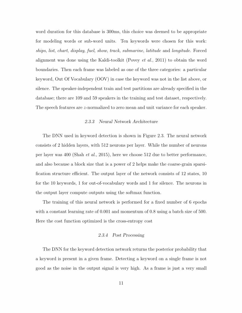
2.3.3 Neural Network Architecture
The DNN used in keyword detection is shown in Figure 2.3. The neural network
consists of 2 hidden layers, with 512 neurons per layer. While the number of neurons
per layer was 400 (Shah et al., 2015), here we choose 512 due to better performance,
and also because a block size that is a power of 2 helps make the coarse-grain sparsi-
fication structure efficient. The output layer of the network consists of 12 states, 10
for the 10 keywords, 1 for out-of-vocabulary words and 1 for silence. The neurons in
the output layer compute outputs using the softmax function.
The training of this neural network is performed for a fixed number of 6 epochs
with a constant learning rate of 0.001 and momentum of 0.8 using a batch size of 500.
Here the cost function optimized is the cross-entropy cost
2.3.4 Post Processing
The DNN for the keyword detection network returns the posterior probability that
a keyword is present in a given frame. Detecting a keyword on a single frame is not
good as the noise in the output signal is very high. As a frame is just a very small
11

Figure 2.3: Neural network architecture for keyword detection consists of 2 hidden
layers with 512 neurons per layer. The input feature dimension is 403 and the output
dimension is 12 (10 keywords, 1 OOV and 1 silence).
sample of the speech signal, a keyword is likely to span multiple frames and as such
the output signal consists of spikes. To reduce the noise in estimation, the estimates
are smoothed using a moving average window of W frames. Another sliding window
of size C is applied over the smoothed estimates, and if the average probability over
the window is greater than a certain threshold the keyword, is said to be present.
The values of W and C are varied to find the optimal value. The optimal values were
found to be W = 50 and C = 25(Shah et al., 2015).
2.3.5 Evaluation
In keyword detection, there can be cases where the system predicts that a keyword
is present (True Positive) or predicts that a keyword is absent (False Alarm). A good
metric to measure the performance of such system is the area under the curve (AUC)
of the receiver operator characteristics (ROC) curve (Bradley, 1997). The ROC is
the plot between rate of true positive detection and rate of false alarms. The area
under this curve represent the probability that the detection system chooses a true
positive case over a false alarm.
12

2.4 Speech Recognition
2.4.1 Input Features
Feature space Maximum Likelihood Linear Regression (fMLLR) is widely used in
speech recognition technologies for speaker adaptation. The fMLLR features (Rath
et al., 2013) are extracted by applying certain transformations on the MFCC features
of the speech signal. Six frames from the neighbourhood of the current frame (3 past
frames and 3 future frames) are chosen and the MFCC features of these frames are
augmented to the MFCC features of the current frame totalling 13*7 =91 features.
These features are then reduced to 40 features by de-correlation and dimensionality
reduction using Linear Discriminant Analysis (LDA). These features are further de-
correlated using the Maximum Likelihood Linear Transform (MLLT). The fMMLR
features can further be spliced in time (5 future frames and 5 past frames) to obtain
the final feature vector for each frame in the speech signal. In this thesis, the features
are obtained by using Kaldi-toolkit (Povey et al., 2011) and the Kaldi and PDNN
scripts (Miao, 2014).
2.4.2 Neural Network Architecture
The DNN used for the speech recognition system is shown in Figure 2.4. This
system consists of 4 hidden layers with 1024 neurons per layer. The output of the
neural network consists of 1483 HMM states obtained from the baseline GMM-HMM
model for the speech recognition system. Similar to the DNN used for keyword
detection, the outputs of neurons in the hidden layers are computed using a ReLU
activation and the neurons in the output layer use the softmax function to compute
the outputs.
The training for this network is performed using a “newbob” approach (Ooi et al.,
13
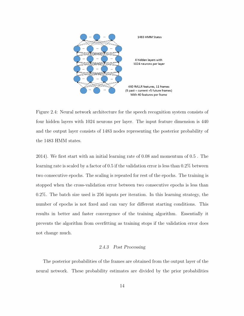
Figure 2.4: Neural network architecture for the speech recognition system consists of
four hidden layers with 1024 neurons per layer. The input feature dimension is 440
and the output layer consists of 1483 nodes representing the posterior probability of
the 1483 HMM states.
2014). We first start with an initial learning rate of 0.08 and momentum of 0.5 . The
learning rate is scaled by a factor of 0.5 if the validation error is less than 0.2% between
two consecutive epochs. The scaling is repeated for rest of the epochs. The training is
stopped when the cross-validation error between two consecutive epochs is less than
0.2%. The batch size used is 256 inputs per iteration. In this learning strategy, the
number of epochs is not fixed and can vary for different starting conditions. This
results in better and faster convergence of the training algorithm. Essentially it
prevents the algorithm from overfitting as training stops if the validation error does
not change much.
2.4.3 Post Processing
The posterior probabilities of the frames are obtained from the output layer of the
neural network. These probability estimates are divided by the prior probabilities
14

that were obtained for each state from the baseline GMM-HMM model (Bourlard
and Morgan, 1994). The scaled estimates are then fed to the Viterbi algorithm to
determine the best sequence of phonemes. These phonemes are then used to transcribe
the words and sentences for the particular input sequence. The post processing of
the neural network output is done using the scripts for the database provided by the
Kaldi-toolkit.
2.4.4 Evaluation
To evaluate different speech recognition implementations, we use the Word Error
Rate (WER) (Morris et al., 2004) metric. WER is derived from Levenshtien distance,
which works at the word level instead of the phoneme level. It is measured as
WER = 100 ∗ (S + D + I)
N(2.8)
where S is the number of substitutions, D is the number of deletions, I is the number
of insertions and N is the number of reference words. In the RM database, the
test portion contains 1460 sentences. While the error rates are for the whole system
(neural network + HMM), the analysis here focuses only on the neural network part.
2.5 Simulation Setup
For the purpose of developing the speech recognition and keyword detection neural
networks, the RM database (Price et al., 1988) is used. This database consists of
sentences recorded in a naval resource management task. It consists of 160 speakers
(70% male and 30% female evenly over four geographic locations NE-NY, Midland,
South, North-West) with varied dialects. The Kaldi toolkit (Povey et al., 2011) is used
to train the speech recognition models. The Kaldi-toolkit is an open source software to
train speech recognition models. This toolkit provides command line tools to perform
15

various operations including training, decoding and evaluating speech models. The
scripts for training the speech models on popular databases are also provided with
the toolkit.
16

Chapter 3
FIXED POINT ARCHITECTURE AND WEIGHT PRUNING
Previous research into reduction of memory for neural network for resource con-
strained hardware involved using a fixed-point architecture to represent values of
weights and biases (Shah et al., 2015). The precision of the weights and biases were
kept constant throughout the network for ease of implementation. To further reduce
the memory, this thesis proposes to use two sets of precision levels one higher pre-
cision and one lower precision level. In this chapter, first a fixed point architecture
with constant precision for keyword detection and speech recognition is presented,
and then the pruning algorithm that results in minimal degradation in performance
is described.
3.1 Fixed-Point NN for Keyword Detection
The neural network for keyword detection consists of two hidden layers with 512
neurons per layer and a output layer with 12 neurons. The input layer consists of 403-
D MFCC features. A floating point architecture of this network requires 1.81MB of
memory. To reduce this memory requirement, the weights, biases and neuron outputs
are represented in fixed-point with fewer bits while keeping the performance of the
system comparable to the floating point architecture. The technique to implement
the fixed-point architecture is as follows.
First, the precision of the weights and biases of the network are determined. In
this step, the neurons in all the layers are kept at 32-bit floating point precision.
The ROC curves for floating point implementations with different number of neu-
rons per hidden layer (256, 512 and 1024 neurons) are shown in Figure 3.1. We see
17
0.0 0.2 0.4 0.6 0.8 1.0
0.0
0.2
0.4
0.6
0.8
1.0
True
Pos
itive
Rat
e
False Alarm Rate
1024 512 256
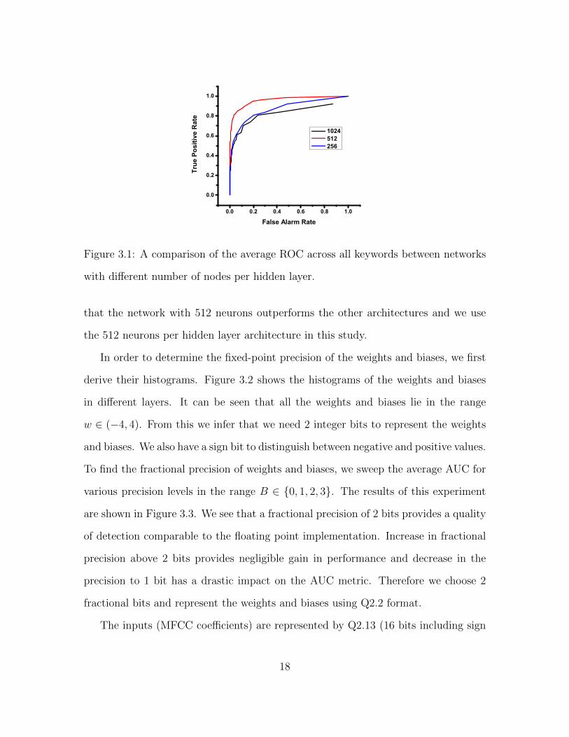
Figure 3.1: A comparison of the average ROC across all keywords between networks
with different number of nodes per hidden layer.
that the network with 512 neurons outperforms the other architectures and we use
the 512 neurons per hidden layer architecture in this study.
In order to determine the fixed-point precision of the weights and biases, we first
derive their histograms. Figure 3.2 shows the histograms of the weights and biases
in different layers. It can be seen that all the weights and biases lie in the range
w ∈ (−4, 4). From this we infer that we need 2 integer bits to represent the weights
and biases. We also have a sign bit to distinguish between negative and positive values.
To find the fractional precision of weights and biases, we sweep the average AUC for
various precision levels in the range B ∈ {0, 1, 2, 3}. The results of this experiment
are shown in Figure 3.3. We see that a fractional precision of 2 bits provides a quality
of detection comparable to the floating point implementation. Increase in fractional
precision above 2 bits provides negligible gain in performance and decrease in the
precision to 1 bit has a drastic impact on the AUC metric. Therefore we choose 2
fractional bits and represent the weights and biases using Q2.2 format.
The inputs (MFCC coefficients) are represented by Q2.13 (16 bits including sign
18

-5 0 50
2000
4000Layer #1 Weights
-0.5 0 0.50
50
100Layer #1 Bias
-5 0 50
2000
4000Layer #2 Weights
-0.025 -0.02 -0.015 -0.01 -0.005 00
50
100Layer #2 Bias
-4 -3 -2 -1 0 1 2 30
200
400Layer #3 Weights
-0.04 -0.02 0 0.02 0.04 0.060
5
10Layer #3 Bias
Figure 3.2: Histogram of weights and biases for keyword detection neural network
0 1 2 3 40.86
0.87
0.88
0.89
0.90
0.91
0.92
0.93
0.94
0.95
Ave
rage
AU
C
Fractional Precision
Figure 3.3: Effect of fractional precision of weights and biases on the average AUC
for keyword detection network
19
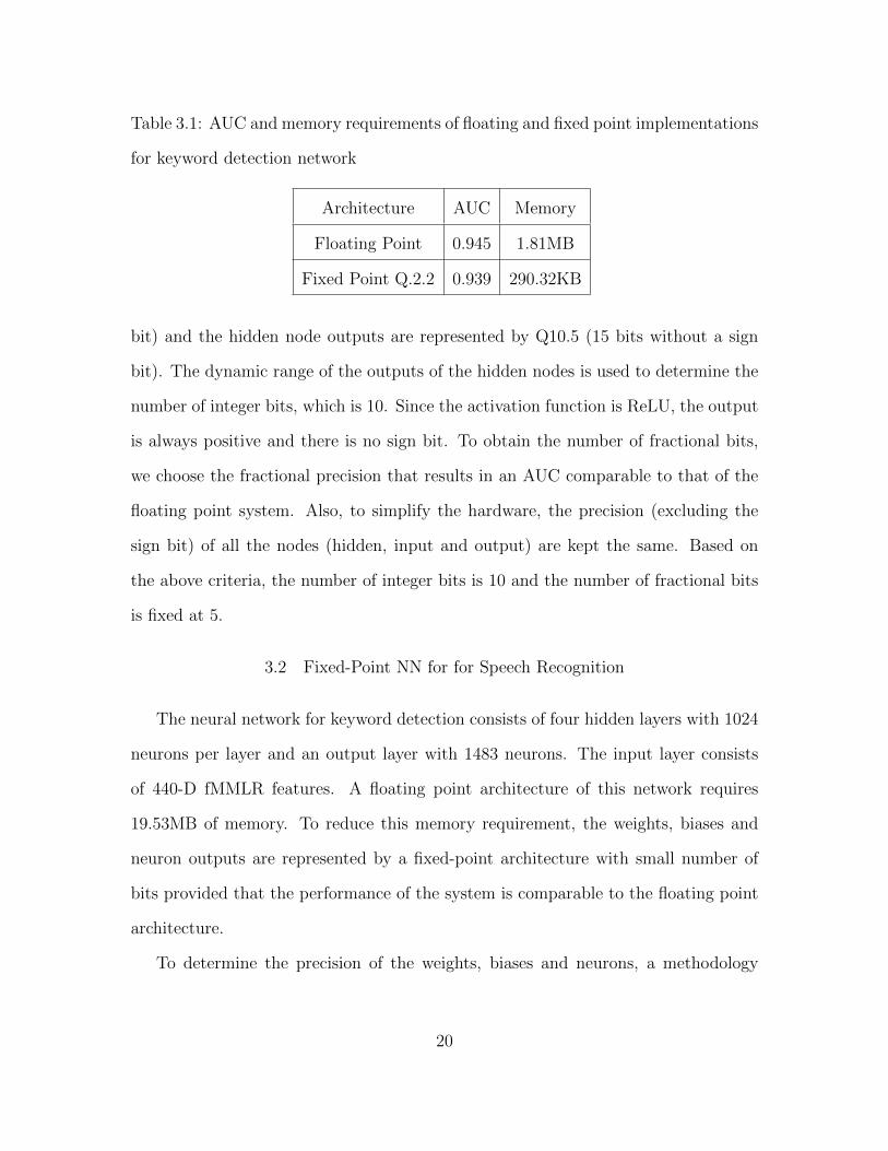
Table 3.1: AUC and memory requirements of floating and fixed point implementations
for keyword detection network
Architecture AUC Memory
Floating Point 0.945 1.81MB
Fixed Point Q.2.2 0.939 290.32KB
bit) and the hidden node outputs are represented by Q10.5 (15 bits without a sign
bit). The dynamic range of the outputs of the hidden nodes is used to determine the
number of integer bits, which is 10. Since the activation function is ReLU, the output
is always positive and there is no sign bit. To obtain the number of fractional bits,
we choose the fractional precision that results in an AUC comparable to that of the
floating point system. Also, to simplify the hardware, the precision (excluding the
sign bit) of all the nodes (hidden, input and output) are kept the same. Based on
the above criteria, the number of integer bits is 10 and the number of fractional bits
is fixed at 5.
3.2 Fixed-Point NN for for Speech Recognition
The neural network for keyword detection consists of four hidden layers with 1024
neurons per layer and an output layer with 1483 neurons. The input layer consists
of 440-D fMMLR features. A floating point architecture of this network requires
19.53MB of memory. To reduce this memory requirement, the weights, biases and
neuron outputs are represented by a fixed-point architecture with small number of
bits provided that the performance of the system is comparable to the floating point
architecture.
To determine the precision of the weights, biases and neurons, a methodology
20
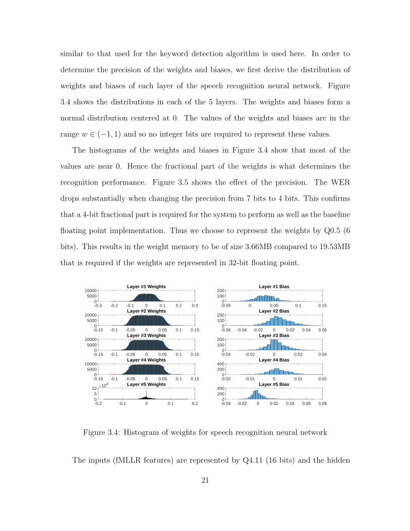
similar to that used for the keyword detection algorithm is used here. In order to
determine the precision of the weights and biases, we first derive the distribution of
weights and biases of each layer of the speech recognition neural network. Figure
3.4 shows the distributions in each of the 5 layers. The weights and biases form a
normal distribution centered at 0. The values of the weights and biases are in the
range w ∈ (−1, 1) and so no integer bits are required to represent these values.
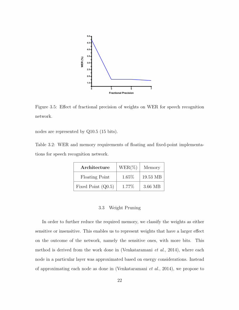
The histograms of the weights and biases in Figure 3.4 show that most of the
values are near 0. Hence the fractional part of the weights is what determines the
recognition performance. Figure 3.5 shows the effect of the precision. The WER
drops substantially when changing the precision from 7 bits to 4 bits. This confirms
that a 4-bit fractional part is required for the system to perform as well as the baseline
floating point implementation. Thus we choose to represent the weights by Q0.5 (6
bits). This results in the weight memory to be of size 3.66MB compared to 19.53MB
that is required if the weights are represented in 32-bit floating point.
-0.3 -0.2 -0.1 0 0.1 0.2 0.30
500010000
Layer #1 Weights
-0.15 -0.1 -0.05 0 0.05 0.1 0.150
500010000
Layer #2 Weights
-0.15 -0.1 -0.05 0 0.05 0.1 0.150
500010000
Layer #3 Weights
-0.15 -0.1 -0.05 0 0.05 0.1 0.150
500010000
Layer #4 Weights
-0.2 -0.1 0 0.1 0.2
×104
05
10Layer #5 Weights
-0.05 0 0.05 0.1 0.150
100200
Layer #1 Bias
-0.06 -0.04 -0.02 0 0.02 0.04 0.060
100200
Layer #2 Bias
-0.04 -0.02 0 0.02 0.040
100200
Layer #3 Bias
-0.02 -0.01 0 0.01 0.020
200400
Layer #4 Bias
-0.04 -0.02 0 0.02 0.04 0.06 0.080
200400
Layer #5 Bias
Figure 3.4: Histogram of weights for speech recognition neural network
The inputs (fMLLR features) are represented by Q4.11 (16 bits) and the hidden
21
4 5 6 7
1.5
2.0
2.5
3.0
3.5
4.0
4.5
5.0
WER
(%)
Fractional Precision
Figure 3.5: Effect of fractional precision of weights on WER for speech recognition
network.
nodes are represented by Q10.5 (15 bits).
Table 3.2: WER and memory requirements of floating and fixed-point implementa-
tions for speech recognition network.
Architecture WER(%) Memory
Floating Point 1.65% 19.53 MB
Fixed Point (Q0.5) 1.77% 3.66 MB
3.3 Weight Pruning
In order to further reduce the required memory, we classify the weights as either
sensitive or insensitive. This enables us to represent weights that have a larger effect
on the outcome of the network, namely the sensitive ones, with more bits. This
method is derived from the work done in (Venkataramani et al., 2014), where each
node in a particular layer was approximated based on energy considerations. Instead
of approximating each node as done in (Venkataramani et al., 2014), we propose to
22
approximate the weights that aids in reducing the memory footprint.
To derive such an architecture, we need to first identify which connections are
sensitive. We achieve weight approximation by piggy-backing on the well known back
propagation algorithm that calculates the gradients at different levels of the network
by back tracking from the output. We train the network by minimizing the cross-
entropy error as described in Section 2.2. Once the trained network is obtained, we
once again use the back propagation algorithm on a sample of M inputs to reduce the
bias and compensate for bad predictions during classification. In our experiments, we
choose the value of M to be 100,000. The errors are used to determine the sensitivity
of the connection. In a specific layer, if the error for a particular weight/bias is greater
than the threshold, we classify the weight as sensitive and use more bits to represent
the value; if the error is below a threshold we deem the weight to be insensitive and
we use fewer bits to represent its value. We sweep the threshold values and determine
the value that results in minimal loss in quality. No retraining is necessary here as
the error produced by incremental retraining will not be high enough to update the
already approximated weights.
3.3.1 Results
The above mentioned pruning algorithm is implemented on both the keyword
detection and speech recognition neural networks.
In the keyword detection neural network, described in Section 3.1, the weights and
biases were represented using Q2.2 format. In order to further reduce the memory
requirement, the sensitive weights and biases are represented using Q2.2 and the
insensitive weights and biases are represented using Q2.1. Figure 4.2 shows the effect
of threshold on the average AUC of such an implementation. For a threshold of 0.4,
52,611 weights and biases are represented using Q2.1 out of a total of 475,660 format
23

resulting in a total memory of 283.89KB.
0.0 0.2 0.4 0.6 0.8 1.00.910
0.915
0.920
0.925
0.930
0.935
0.940
0.945
Ave
rage
AU
C
Threshold
Figure 3.6: Effect of threshold on AUC for keyword detection neural network
In the speech recognition neural network, described in Section 3.2, the weights and
biases were represented using Q0.5 format. In order to further reduce the memory
requirement, the sensitive weights and biases are represented using Q0.5 and the
insensitive weights and biases are represented using Q0.4. Figure 3.7 shows the effect
of threshold on the average AUC of such an implementation. For a threshold of 0.4,
226,791 weights and biases are represented using Q0.4 out of a total of 5,120,459
resulting in memory size of 3.63MB.
Table 3.3: Memory Requirement of Networks with Pruned Weights.
Network Memory Performance
Keyword Detection 283.89KB 0.91 (AUC)
Speech Recognition 3.63MB 1.82%(WER)
The results for the weight pruning algorithm are tabulated in Table 3.3. We see
that the keyword detection and speech recognition networks perform with minimal
24

0.0 0.2 0.4 0.6 0.8 1.01.5
2.0
2.5
3.0
3.5
4.0
4.5
5.0
WER
Threshold
Figure 3.7: Effect of weight pruning threshold on WER for speech recognition net-
work.
degradation of performance with a memory reduction of 0.82% and 2.12%, respec-
tively.
3.4 Conclusions
In this chapter a fully-connected feed-forward fixed point neural network architec-
ture was presented for two key speech applications, namely, keyword detection and
speech recognition. Techniques were developed to represent the weights and biases
with minimum number of bits to reduce the memory footprint while minimally af-
fecting the detection/recognition performance. With a fixed point architecture the
memory requirement of the network was reduced by 83% compared to a naive floating
point architecture. This was achieved by using a fixed point implementation using 5
-7 bits. A weight pruning technique was also presented.
25

Chapter 4
COARSE GRAIN SPARSIFICATION
In this chapter, a hardware-centric methodology to develop neural network with a
small memory footprint and computational requirement is described. Such a design
is achieved by judiciously dropping large blocks of weights. This method, termed
coarse-grain sparsification, resulted in 20x memory compression when tested on neural
network architectures for both keyword detection and speech recognition.
4.1 Overview
The large memory requirement of the neural network is due to the large weight
matrices, which have very large dimensions. For instance, the speech recognition
system uses three weight matrices of size 1024× 1024, and two matrices each of size
1024 × 440 and 1024 × 1483. To reduce memory requirement of a neural network,
some of the weights/connections between the layers can be dropped. The challenge is
to drop a select set that will not affect the performance of the network adversely. The
removal of connections reduces the memory requirement significantly when compared
to the weight pruning algorithm. This is because here we are able to remove all the
bits for the weights instead of removing only 1 or 2 bits from the weights as in the
weight pruning algorithm.
In the rest of this chapter, the coarse-grain sparsification(CGS) technique, that
efficiently compresses the memory, is presented. The key idea here is to drop the
connections in large blocks (e.g., 64× 64, 128× 128), and enforce such a constraint in
a static manner throughout the training phase of the algorithm. The remaining con-
nections of the network can be efficiently mapped onto SRAM arrays with minimal
26

address information for classification. The blocks of connections are removed with a
certain probability (e.g. 75%) during the initialization of the network and this struc-
ture is kept constant throughout training and classification phases. This structure
is different from the Dropout (Srivastava et al., 2014) and Dropconnect (Wan et al.,
2013) architecture that are commonly used in deep learning algorithms to prevent
overfitting. Dropout and Dropconnect drop nodes or weights in a dynamic manner
in every training iteration. Since the removal of the weights/nodes is dynamic, these
approaches do not aid in reducing the memory footprint of the network and the fully
connected network is required during classification.
4.2 Block Structure
There exists prior work on partially connected neural networks where some con-
nections between layers have been dropped. Previous approaches drop the weights
based on a specific criteria (e.g. if the value is lower than a threshold). Such an
approach prevents efficient mapping onto hardware since the weights, as well as the
indices of the non-zero weights, have to be stored. To overcome this inefficiency, in our
technique, the connections are dropped in large blocks and the weights are dropped
on a block-by-block basis. A fully-connected neural network is first initialized and
then a certain percentage of the connections are removed block-by-block keeping the
number of remaining blocks (e.g. 50%, 75%) constant along either the row or col-
umn dimension. Throughout training and classification, the weights in the dropped
blocks remain zero. This ensures that there is no memory allocated for these dropped
connections, resulting in reduced memory footprint.
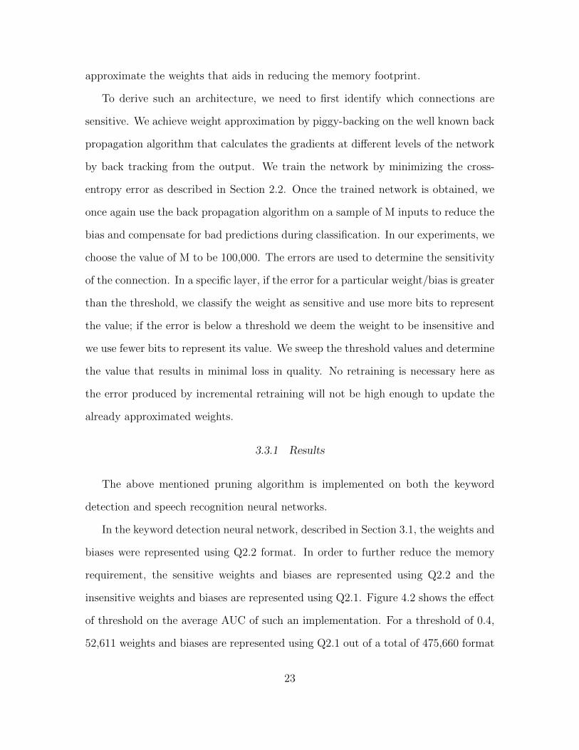
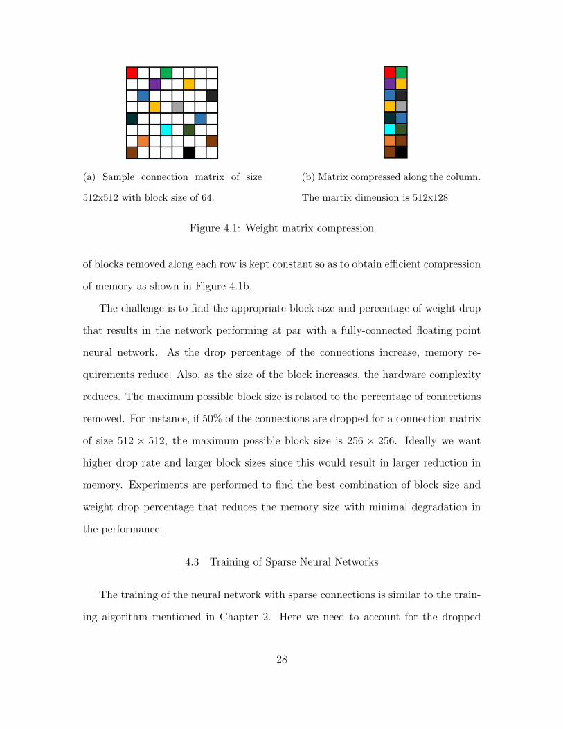
Figure 4.1a shows a sample connection matrix with size of 512× 512. The matrix
is divided into 64 blocks each of size 64×64. The white blocks indicate the absence of
connections and the colored blocks indicate the presence of connections. The number
27
(a) Sample connection matrix of size
512x512 with block size of 64.
(b) Matrix compressed along the column.
The martix dimension is 512x128
Figure 4.1: Weight matrix compression
of blocks removed along each row is kept constant so as to obtain efficient compression
of memory as shown in Figure 4.1b.
The challenge is to find the appropriate block size and percentage of weight drop
that results in the network performing at par with a fully-connected floating point
neural network. As the drop percentage of the connections increase, memory re-
quirements reduce. Also, as the size of the block increases, the hardware complexity
reduces. The maximum possible block size is related to the percentage of connections
removed. For instance, if 50% of the connections are dropped for a connection matrix
of size 512 × 512, the maximum possible block size is 256 × 256. Ideally we want
higher drop rate and larger block sizes since this would result in larger reduction in
memory. Experiments are performed to find the best combination of block size and
weight drop percentage that reduces the memory size with minimal degradation in
the performance.
4.3 Training of Sparse Neural Networks
The training of the neural network with sparse connections is similar to the train-
ing algorithm mentioned in Chapter 2. Here we need to account for the dropped
28
connections when performing the forward propagation and the back-propagation in
the training algorithm. A connection matrix C is introduced, where the element Cij
is a binary variable that represents a connection between ith neuron in one layer and
jth neuron in another layer. The connection matrix can take values of either one or
zero depending on whether a connection between the neurons across adjacent layers
is present or absent.
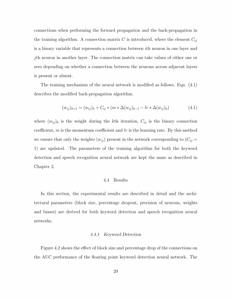
The training mechanism of the neural network is modified as follows. Eqn. (4.1)
describes the modified back-propagation algorithm.
(wij)k+1 = (wij)k + Cij ∗ (m ∗∆(wij)k−1 − lr ∗∆(wij)k) (4.1)
where (wij)k is the weight during the kth iteration, Cij is the binary connection
coefficient, m is the momentum coefficient and lr is the learning rate. By this method
we ensure that only the weights (wij) present in the network corresponding to (Cij =
1) are updated. The parameters of the training algorithm for both the keyword
detection and speech recognition neural network are kept the same as described in
Chapter 2.
4.4 Results
In this section, the experimental results are described in detail and the archi-
tectural parameters (block size, percentage dropout, precision of neurons, weights
and biases) are derived for both keyword detection and speech recognition neural
networks.
4.4.1 Keyword Detection
Figure 4.2 shows the effect of block size and percentage drop of the connections on
the AUC performance of the floating point keyword detection neural network. The
29

1x1 2x2 4x4 8x8 16x1632x3264x64128x1280.800.820.840.860.880.900.920.940.960.98
Ave
rage
AU
C
Block Size
25% weight drop 50% weight drop 75% weight drop 88% weight drop
Figure 4.2: Effect of block size and percentage dropout on WER of speech recognition
network
percentage drop of the connections are with respect to the two middle layers. We
do not drop connections in the last layer since it consists of only 12 nodes and is
relatively sensitive. Also since the last layer contributes to 1% of the total weights
in the system, any reduction in this layer does not result in substantial reduction in
memory requirement. From Figure 4.2, we see that for the same block size, increasing
the percentage of dropped connections adversely affects the AUC performance, as
expected. When the drop in connections is less than 50%, there is little change in the
AUC performance even when the block size is large. However, for larger drops, the
AUC performance becomes sensitive to the block size. For instance, the performance
of a system with 75% of its weights dropped has an AUC performance loss of up to
0.029 when the block size is 128×128. The AUC performance loss is only 0.015 when
the block size is 64× 64, and so we use this configuration in our sparse network.
To determine the fixed point precision of the CGS architecture for keyword de-
30
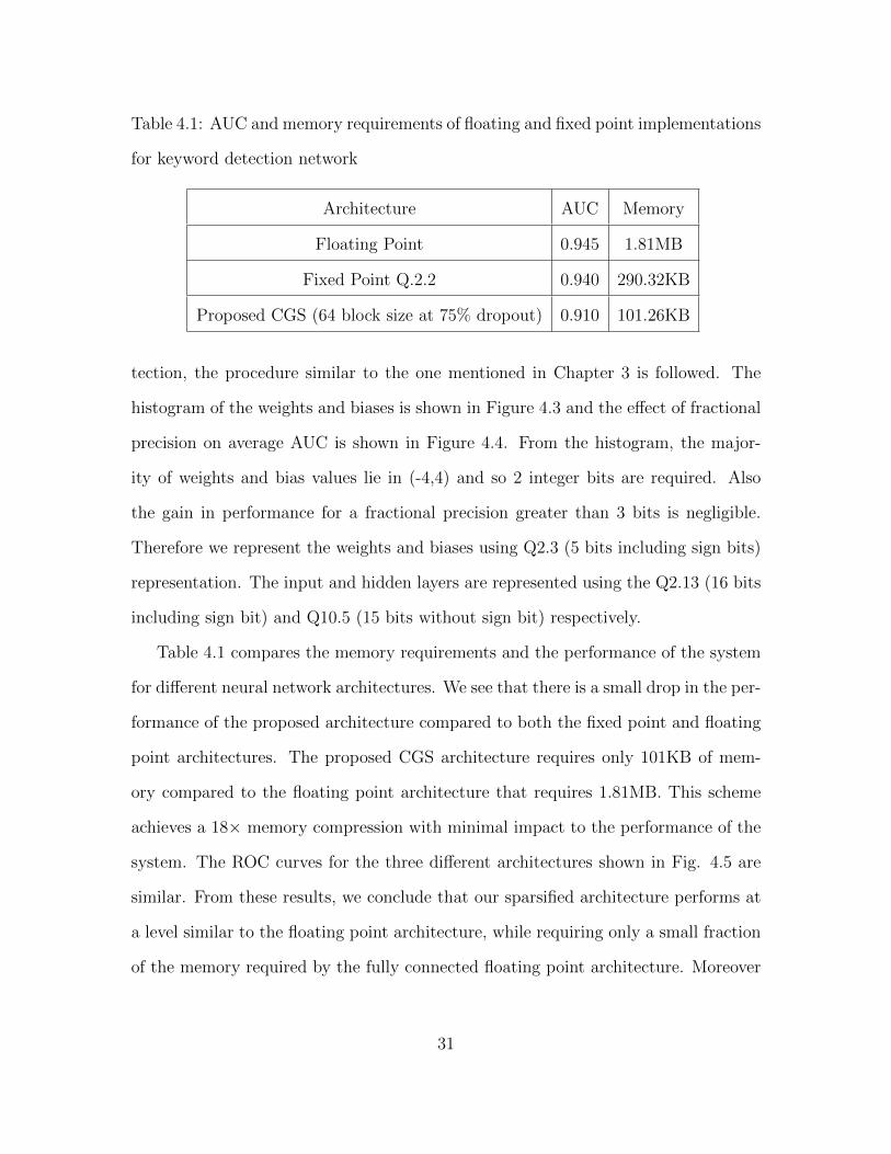
Table 4.1: AUC and memory requirements of floating and fixed point implementations
for keyword detection network
Architecture AUC Memory
Floating Point 0.945 1.81MB
Fixed Point Q.2.2 0.940 290.32KB
Proposed CGS (64 block size at 75% dropout) 0.910 101.26KB
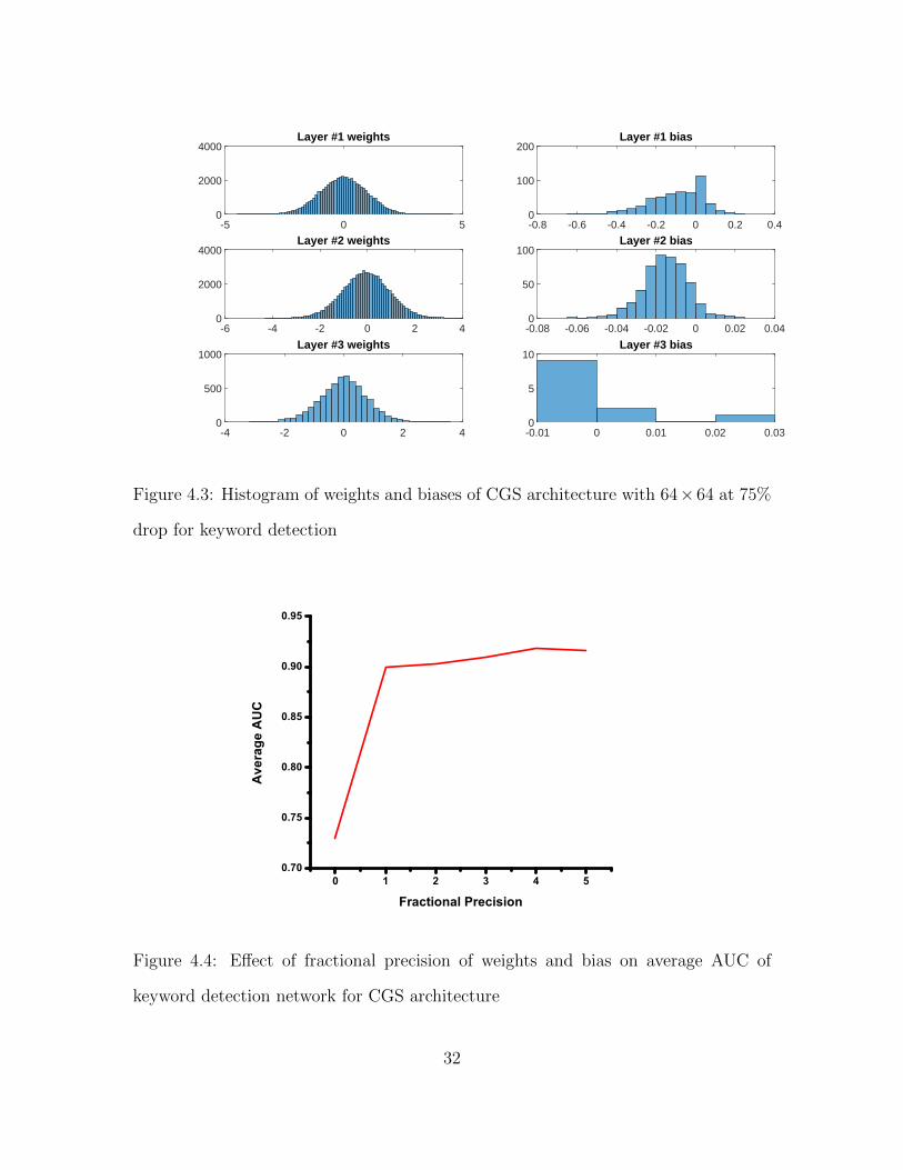
tection, the procedure similar to the one mentioned in Chapter 3 is followed. The
histogram of the weights and biases is shown in Figure 4.3 and the effect of fractional
precision on average AUC is shown in Figure 4.4. From the histogram, the major-
ity of weights and bias values lie in (-4,4) and so 2 integer bits are required. Also
the gain in performance for a fractional precision greater than 3 bits is negligible.
Therefore we represent the weights and biases using Q2.3 (5 bits including sign bits)
representation. The input and hidden layers are represented using the Q2.13 (16 bits
including sign bit) and Q10.5 (15 bits without sign bit) respectively.
Table 4.1 compares the memory requirements and the performance of the system
for different neural network architectures. We see that there is a small drop in the per-
formance of the proposed architecture compared to both the fixed point and floating
point architectures. The proposed CGS architecture requires only 101KB of mem-
ory compared to the floating point architecture that requires 1.81MB. This scheme
achieves a 18× memory compression with minimal impact to the performance of the
system. The ROC curves for the three different architectures shown in Fig. 4.5 are
similar. From these results, we conclude that our sparsified architecture performs at
a level similar to the floating point architecture, while requiring only a small fraction
of the memory required by the fully connected floating point architecture. Moreover
31
-5 0 50
2000
4000Layer #1 weights
-6 -4 -2 0 2 40
2000
4000Layer #2 weights
-4 -2 0 2 40
500
1000Layer #3 weights
-0.8 -0.6 -0.4 -0.2 0 0.2 0.40
100
200Layer #1 bias
-0.08 -0.06 -0.04 -0.02 0 0.02 0.040
50
100Layer #2 bias
-0.01 0 0.01 0.02 0.030
5
10Layer #3 bias
Figure 4.3: Histogram of weights and biases of CGS architecture with 64×64 at 75%
drop for keyword detection
0 1 2 3 4 50.70
0.75
0.80
0.85
0.90
0.95
Ave
rage
AU
C
Fractional Precision
Figure 4.4: Effect of fractional precision of weights and bias on average AUC of
keyword detection network for CGS architecture
32

0.0 0.5 1.00.0
0.5
1.0
True
Pos
itive
Rat
e
False Alarm Rate
Proposed CGS with Fixed Point Fully Connected Floating Point Fully Connected Fixed Point
Figure 4.5: ROC Curve of different deep neural network implementations for keyword
detection.
with 75% of the weights dropped, we also achieve a 4× reduction in the number of
computations, which further reduces the power consumption of the network.
4.4.2 Speech Recognition
Figure 4.6 shows the effect of percentage drop of connections on the WER of the
floating point system as a function of the block size. At up to 75% weight drop at
all layers of the network, the performance of the system is comparable to the fully
connected floating point DNN. Increasing the drop rate to 88% for block sizes larger
than 64× 64, increases the error rate. Based on this analysis, we choose a drop rate
of 75% across all layers with block size of 64× 64.
To determine the fixed point precision of the CGS architecture, the procedure
similar to the one mentioned in Chapter 3 is followed. The histogram of the weights
and biases is shown in Figure 4.7 and the effect of fractional precision on WER is
33

4x4 8x8 16x16 32x32 64x64 128x128256x256
1.6
1.7
1.8
1.9
2.0
2.1
2.2
WER
(%)
Block Size
75% Drop 50% Drop 88% Drop
Figure 4.6: Effect of block size and percentage dropout on WER of speech recognition
network
shown in Figure 4.8. From the histogram, we see that the majority of weights and bias
values lie in (-1,1) and so 0 integer bits are required. Also the gain in performance
for a fractional precision greater than 4 bits is negligible. Therefore we represent the
weights and biases using Q0.4 (5 bits including sign bits) representation. The input
and hidden layers are represented using Q4.11 (16 bits including sign bit) and Q10.5
(15 bits without sign bit) respectively.
Table 4.2 compares the performance of our system with the fully connected floating
point and fixed point architectures. The sparse fixed-point DNN using the proposed
technique with up to 75% of its connections dropped, has an WER close to that of
the floating point fully-connected DNN. The proposed architecture requires memory
size of only 0.85MB compared to 19.53MB of a fully connected floating point archi-
tecture. Thus, the sparsified fixed point network is able to drop ∼95% of the memory
requirement with a small drop in performance. Moreover, with 75% of the weights
34

-1.5 -1 -0.5 0 0.5 1 1.50
20004000
Layer #1 Weights
-1 -0.5 0 0.5 10
500010000
Layer #2 Weights
-0.6 -0.4 -0.2 0 0.2 0.40
5000Layer #3 Weights
-0.6 -0.4 -0.2 0 0.2 0.4 0.60
500010000
Layer #4 Weights
-1 -0.5 0 0.5 1
×104
012
Layer #5 Weights
-2 -1 0 1 20
100200
Layer #1 Bias
-0.5 0 0.5 10
200400
Layer #2 Bias
-0.4 -0.2 0 0.2 0.4 0.60
200400
Layer #3 Bias
-0.2 -0.1 0 0.1 0.2 0.30
200400
Layer #4 Bias
-0.5 0 0.5 1 1.50
200400
Layer #5 Bias
Figure 4.7: Histogram of weights and biases of CGS architecture with 64×64 at 75%
drop
2 3 4 5 6 7
0
10
20
30
40
50
60
WER
Fractional Precision
Figure 4.8: Effect of fractional precision of weights and bias on WER of speech
recognition system for CGS architecture
35
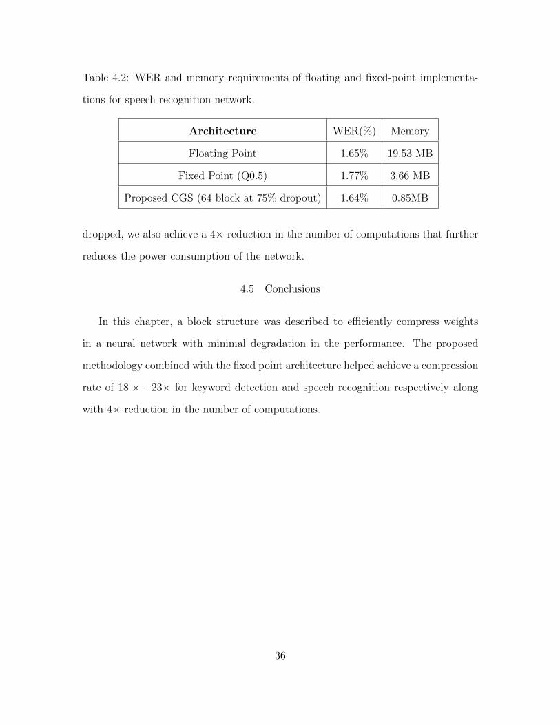
Table 4.2: WER and memory requirements of floating and fixed-point implementa-
tions for speech recognition network.
Architecture WER(%) Memory
Floating Point 1.65% 19.53 MB
Fixed Point (Q0.5) 1.77% 3.66 MB
Proposed CGS (64 block at 75% dropout) 1.64% 0.85MB
dropped, we also achieve a 4× reduction in the number of computations that further
reduces the power consumption of the network.
4.5 Conclusions
In this chapter, a block structure was described to efficiently compress weights
in a neural network with minimal degradation in the performance. The proposed
methodology combined with the fixed point architecture helped achieve a compression
rate of 18 × −23× for keyword detection and speech recognition respectively along
with 4× reduction in the number of computations.
36
Chapter 5
CONCLUSIONS
5.1 Summary
This thesis focused on developing techniques to reduce the memory size in deep
networks, specifically in feed-forward neural networks for keyword detection and
speech recognition. The neural network for keyword detection consists of 2 hidden
layers, with 512 neurons per layer, while the network for speech recognition is much
larger with 4 hidden layers and 1024 neurons per layer.
First, techniques were developed to represent the weights and biases with mini-
mum number of bits to reduce the memory footprint while minimally affecting the
detection/recognition performance. For keyword detection, where 10 keywords were
selected from the RM corpus, experimental results show that there is only a marginal
loss in performance when the weights are stored in Q2.2 (5 bits) format. The to-
tal memory required in this case is approximately 290KB (compared to 1.81MB if
the weights were represented by 32 bit floating point), making it highly suitable for
resource constrained hardware devices. On the larger speech recognition network,
the memory reduction is even more significant. Here the memory size dropped from
19.53MB to 3.66MB when the weights are represented in Q0.5 (6 bits) format. An
additional 0.82%-2.12% reduction (compared to fixed point implementation) can be
obtained by representing insensitive weights by lower precision.
Even larger reduction in memory was achieved by dropping connections in blocks.
Instead of reducing the precision levels of the individual weights, here the weight
connections are removed from the network. We show that the keyword detection
37
and speech recognition networks with 75% of its connections removed performs at
a level similar to that of fully connected networks. Application of this technique on
fixed point reduced precision implementation, helped reduce the memory requirement
by ∼95% compared to a fully connected double precision floating point architecture.
Such an architecture also reduces the number of computations by 4×. Therefore, these
proposed techniques can substantially reduce the memory and power requirement
of resource-constrained devices. As speech recognition becomes more mainstream,
the proposed techniques will enable implementation of these networks in mobile and
wearable devices.
5.2 Future Work
Future work in this area can be directed towards finding an optimal block selection
that maximizes the accuracy of the system. Other approaches include implementing
Convolutional Neural Networks (Abdel-Hamid et al., 2014) to analyze the input fea-
tures. Recently Recurrent Neural Networks (Graves and Jaitly, 2014) have been
shown to perform comparable to DNN-HMM systems. These networks have greatly
simplified the speech recognition pipeline. Implementing the proposed memory re-
duction schemes on RNNs can simplify their hardware implementations significantly.
38
REFERENCES
Abdel-Hamid, O., A.-R. Mohamed, H. Jiang, L. Deng, G. Penn and D. Yu, “Con-volutional neural networks for speech recognition,” IEEE/ACM Transactions onAudio, Speech, and Language Processing 22, 10, 1533–1545 (2014).
Baker, J. M., L. Deng, J. Glass, S. Khudanpur, C.-H. Lee, N. Morgan and D. O.Shaughnessy, “Developments and directions in speech recognition and understand-ing, Part 1 [dsp education],” Signal Processing Magazine, IEEE 26, 3, 75–80 (2009).
Bourlard, H. A. and N. Morgan, Connectionist speech recognition: a hybrid approach,vol. 247 (Springer Science & Business Media, 1994).
Bradley, A. P., “The use of the area under the roc curve in the evaluation of machinelearning algorithms,” Pattern recognition 30, 7, 1145–1159 (1997).
Chen, G., C. Parada and G. Heigold, “Small-footprint keyword spotting using deepneural networks,” in IEEE International Conference on Acoustics, Speech and Sig-nal Processing (ICASSP), pp. 4087–4091 (2014).
Dahl, G. E., D. Yu, L. Deng and A. Acero, “Large vocabulary continuous speechrecognition with context-dependent DBN-HMMs,” in IEEE International Confer-ence on Acoustics, Speech and Signal Processing (ICASSP), pp. 4688–4691, (2011).
Dahl, G. E., D. Yu, L. Deng and A. Acero, “Context-dependent pre-trained deepneural networks for large-vocabulary speech recognition,” IEEE Transactions onAudio, Speech, and Language Processing 20, 1, 30–42 (2012).
Deng, L. and D. Yu, “Deep learning: Methods and applications,” Foundations andTrends in Signal Processing 7, 3–4, 197–387 (2014).
Gales, M. and S. Young, “The application of hidden Markov models in speech recog-nition,” Foundations and trends in signal processing 1, 3, 195–304 (2008).
Gardner, W. A., “Learning characteristics of stochastic-gradient-descent algorithms:A general study, analysis, and critique,” Signal Processing 6, 2, 113–133 (1984).
Graves, A. and N. Jaitly, “Towards end-to-end speech recognition with recurrentneural networks,” in Proceedings of the 31st International Conference on MachineLearning (ICML-14), pp. 1764–1772 (2014).
Hinton, G., L. Deng, D. Yu, G. E. Dahl, A.-r. Mohamed, N. Jaitly, A. Senior, V. Van-houcke, P. Nguyen, T. N. Sainath et al., “Deep neural networks for acoustic mod-eling in speech recognition: The shared views of four research groups”, SignalProcessing Magazine, IEEE 29, 6, 82–97 (2012).
Huang, X., A. Acero, H.-W. Hon and R. Foreword By-Reddy, Spoken language pro-cessing: A guide to theory, algorithm, and system development (Prentice Hall PTR,2001).
39

Juang, B.-H., S. E. Levinson and M. M. Sondhi, “Maximum likelihood estimationfor multivariate mixture observations of Markov chains,” IEEE Transactions onInformation Theory 32, 2, 307–309 (1986).
Mamou, J., B. Ramabhadran and O. Siohan, “Vocabulary independent spoken termdetection,” in Proceedings of the 30th Annual International ACM SIGIR Confer-ence on Research and Development in Information Retrieval, pp. 615–622 (ACM,2007).
Miao, Y., “Kaldi+ pdnn: building DNN-based ASR systems with Kaldi and PDNN,”arXiv preprint arXiv:1401.6984 (2014).
Miller, D. R., M. Kleber, C.-L. Kao, O. Kimball, T. Colthurst, S. A. Lowe, R. M.Schwartz and H. Gish, “Rapid and accurate spoken term detection,” in INTER-SPEECh, pp. 314-317 (2007).
Morris, A. C., V. Maier and P. D. Green, “From WER and RIL to MER and WIL: im-proved evaluation measures for connected speech recognition,” in INTERSPEECH,pp. 2765-2768 (2004).
Ooi, W. T., C. G. Snoek, H. K. Tan, C. K. Ho, B. Huet and C.-W. Ngo, 15th PacificRim Conference on Advances in Multimedia Information Processing-PCM , vol.8879 (Springer, 2014).
Parlak, S. and M. Saraclar, “Spoken term detection for Turkish broadcast news,”in IEEE International Conference on Acoustics, Speech and Signal Processing,(ICASSP), pp. 5244–5247, (2008).
Povey, D., A. Ghoshal, G. Boulianne, L. Burget, O. Glembek, N. Goel, M. Han-nemann, P. Motlicek, Y. Qian, P. Schwarz et al., “The kaldi speech recognitiontoolkit,” in IEEE 2011 workshop on automatic speech recognition and understand-ing, No. EPFL-CONF-192584 (IEEE Signal Processing Society, 2011).
Price, P., W. M. Fisher, J. Bernstein and D. S. Pallett, “The Darpa 1000-word re-source management database for continuous speech recognition,” in InternationalConference on Acoustics, Speech, and Signal Processing (ICASSP), pp. 651–654(1988).
Rath, S. P., D. Povey, K. Vesely and J. Cernocky, “Improved feature processing fordeep neural networks,” in INTERSPEECH, pp. 109–113 (2013).
Rohlicek, J. R., W. Russell, S. Roukos and H. Gish, “Continuous hidden Markovmodeling for speaker-independent word spotting,” in 1989 International Conferenceon Acoustics, Speech, and Signal Processing, , pp. 627–630, (1989).
Rose, R. C. and D. B. Paul, “A hidden markov model based keyword recognition sys-tem,” in 1990 International Conference on Acoustics, Speech, and Signal Processing(ICASSP), pp. 129–132, (1990).
40
Sha, F. and L. K. Saul, “Large margin Gaussian Mixture Modeling for phoneticclassification and recognition,” in IEEE International Conference on Acoustics,Speech and Signal Processing (ICASSP), vol. 1, pp. I–I (2006).
Shah, M., J. Wang, D. Blaauw, D. Sylvester, H.-S. Kim and C. Chakrabarti, “A fixed-point neural network for keyword detection on resource constrained hardware,” in2015 IEEE Workshop on Signal Processing Systems (SiPS), pp. 1–6 (2015).
Silaghi, M.-C., “Spotting subsequences matching an HMM using the average obser-vation probability criteria with application to keyword spotting,” in Proceedings ofthe American Association on Artificial Intelligence, vol. 20, pp. 1118-1123 (MenloPark, CA; Cambridge, MA; London; AAAI Press; MIT Press; 2005).
Silaghi, M.-C. and H. Bourlard, “Iterative posterior-based keyword spotting with-out filler models,” in Proceedings of the IEEE Automatic Speech Recognition andUnderstanding Workshop, pp. 213–216 (1999).
Song, H. A. and S.-Y. Lee, “Hierarchical representation using NMF,” in Neural In-formation Processing, pp. 466–473 (Springer, 2013).
Srivastava, N., G. Hinton, A. Krizhevsky, I. Sutskever and R. Salakhutdinov,“Dropout: A simple way to prevent neural networks from overfitting,” The Journalof Machine Learning Research 15, 1, 1929–1958 (2014).
Su, D., X. Wu and L. Xu, “GMM-HMM acoustic model training by a two levelprocedure with Gaussian components determined by automatic model selection,”in IEEE International Conference on Acoustics, Speech and Signal Processing(ICASSP), pp. 4890–4893 (2010).
Sutskever, I., J. Martens, G. Dahl and G. Hinton, “On the importance of initial-ization and momentum in deep learning,” in Proceedings of the 30th internationalconference on machine learning (ICML-13), pp. 1139–1147 (2013).
Tomas, J., J. A. Mas and F. Casacuberta, “A quantitative method for machine trans-lation evaluation,” in Proceedings of the EACL 2003 Workshop on Evaluation Ini-tiatives in Natural Language Processing: Are evaluation methods, metrics and re-sources reusable?, pp. 27–34 (Association for Computational Linguistics, 2003).
Van Ooyen, A. and B. Nienhuis, “Improving the convergence of the back-propagationalgorithm”, Neural Networks 5, 3, 465–471 (1992).
Venkataramani, S., A. Ranjan, K. Roy and A. Raghunathan, “Axnn: energy-efficientneuromorphic systems using approximate computing,” in Proceedings of the 2014International Symposium on Low Power Electronics and Design, pp. 27–32 (2014).
Wan, L., M. Zeiler, S. Zhang, Y. L. Cun and R. Fergus, “Regularization of neuralnetworks using dropconnect,” in Proceedings of the 30th International Conferenceon Machine Learning (ICML-13), pp. 1058–1066 (2013).
41

Wilpon, J., L. Miller and P. Modi, “Improvements and applications for key wordrecognition using hidden Markov modeling techniques,” in 1991 International Con-ference on Acoustics, Speech, and Signal Processing,, pp. 309–312, (1991).
Zeiler, M. D., M. Ranzato, R. Monga, M. Mao, K. Yang, Q. V. Le, P. Nguyen,A. Senior, V. Vanhoucke, J. Dean, G. Hinton, “On rectified linear units for speechprocessing,” in 2013 IEEE International Conference on Acoustics, Speech and Sig-nal Processing (ICASSP), pp. 3517–3521, (2013).
42