approximate proximity problems in high dimensions via
TRANSCRIPT

3 April 2007
Approximate Proximity Problems in High Dimensions
via Locality-Sensitive HashingPiotr Indyk

3 April 2007
Closest Pair• We have seen several algorithms for the closest
pair problem over n points in Rd
– d=2: O(n log n)– d>2: dO(d) n (or O(dn2) )
• The exponential dependence on d, a.k.a. “curse of dimensionality”, is a very common phenomenon– See talk by Nina Amenta, 4pm, Kiva/Star
• Next few lectures: how to get around this problem

3 April 2007
Nearest Neighbor• For a set P of n points in Rd
– Nearest Neighbor: for any query q, returns a point p∈P minimizing ||p-q||
– r-Near Neighbor: for any query q, returns a point p∈P s.t. ||p-q|| ≤ r (if it exists)
• If we have data structure with – Construction time T(n)– Query time Q(n)then we can solve r-Close Pair intime [ T(n) + n Q(n) ] log n
• Unfortunately, no algorithm with small T(n) and Q(n) is known
q
r

3 April 2007
Approximate Near Neighbor• c-Approximate r-Near Neighbor: build data
structure which, for any query q: – If there is a point p∈P, ||p-q|| ≤ r– it returns p’∈P, ||p-q|| ≤ cr
• Reductions:– c-Approx r-Close Pair – c-Approx Nearest Neighbor reduces to c-Approx
Near Neighbor (log overhead)
– One can enumerate all approx near neighbors→ can solve exact near neighbor problem
– Other apps: c-approximate Minimum Spanning Tree, clustering, etc.
q
r
cr

3 April 2007
Today
• A c-Approx r-Near Neighbor:– Preprocessing: dn1+1/c
– Query time: dn1/c
– …for binary vectors• Sketch how to improve 1/c to 1/c2+δ

3 April 2007
Locality-Sensitive Hashing
• Idea: construct hash functions g: Rd → U such that for any points p,q:– If ||p-q|| ≤ r, then Pr[g(p)=g(q)]
is “high”– If ||p-q|| >cr, then Pr[g(p)=g(q)]
is “small”• Then we can solve the
problem by hashing
“not-so-small”
q
p

3 April 2007
LSH [Indyk-Motwani’98]
• A family H of functions h: Rd → U is called (P1,P2,r,cr)-sensitive, if for any p,q:– if ||p-q|| <r then Pr[ h(p)=h(q) ] > P1
– if ||p-q|| >cr then Pr[ h(p)=h(q) ] < P2
• Example: Hamming distance– LSH functions: h(p)=pi, i.e., the i-th bit of p– Probabilities: Pr[ h(p)=h(q) ] = 1-D(p,q)/d
p=10010010q=11010110

3 April 2007
LSH Algorithm• We use functions of the form
g(p)=<h1(p),h2(p),…,hk(p)>• Preprocessing:
– Select g1…gL– For all p∈P, hash p to buckets g1(p)…gL(p)
• Query:– Retrieve the points from buckets g1(q), g2(q), … , until
• Either the points from all L buckets have been retrieved, or• Total number of points retrieved exceeds 3L
– Answer the query based on the retrieved points– Total time: O(dL)

3 April 2007
Analysis
• Lemma1: LSH solves c-approximate NN with:– Number of hash fun: L=nρ, ρ=log(1/P1)/log(1/P2)
– Constant success probability per query q• Lemma 2: for LSH functions as seen
earlier we have ρ=1/c

3 April 2007
Proof of Lemma 1 by picture• Points in {0,1}d
• Collision prob. for k=1..3, L=1..3 (recall: L=#indices, k=#h’s )
• Distance ranges from 0 to d=10
0
0.2
0.4
0.6
0.8
1
1.2
1 3 5 7 9 11
Distance
Col
lisio
n pr
obab
ility
k=1
k=2
k=3
0
0.2
0.4
0.6
0.8
1
1.2
1 3 5 7 9 11
Distance
Col
lisio
n Pr
obab
ility
k=1k=2
k=3
0
0.2
0.4
0.6
0.8
1
1.2
1 2 3 4 5 6 7 8 9 10
Distance
Col
lisio
n pr
obab
ility
k=1
k=2
k=3

3 April 2007
Proof
• Define:– p: a point such that ||p-q|| ≤ r– FAR(q)={ p’∈P: ||p’-q|| >c r }– Bi(q)={ p’∈P: gi(p’)=gi(q) }
• Will show that both events occur with >0probability:– E1: gi(p)=gi(q) for some i=1…L– E2: Σi |Bi(q) ∩ FAR(q)| < 3L

3 April 2007
Proof ctd.
• Set k=log1/P2 n• For p’∈FAR(q) ,
Pr[gi(p’)=gi(q)] ≤ P2k =1/n
• E[ |Bi(q)∩FAR(q)| ] ≤ 1• E[Σi |Bi(q)∩FAR(q)| ] ≤ L• Pr[Σi |Bi(q)∩FAR(q)|≥3L ] ≤ 1/3

3 April 2007
Proof, ctd.
• Pr[ gi(p)=gi(q) ] ≥ 1/P1k = 1/nρ =1/L
• Pr[ gi(p)≠gi(q), i=1..L] ≤ (1-1/L)L ≤ 1/e

3 April 2007
Proof, end
• Pr[E1 not true]+Pr[E2 not true] ≤ 1/3+1/e =0.7012.
• Pr[ E1 ∩E2 ] ≥ 1-(1/3+1/e) ≈0.3

3 April 2007
Proof of Lemma 2
• Statement: for – P1=1-r/d– P2=1-cr/d
we have ρ=log(P1)/log(P2) ≤ 1/c• Proof:
– Need P1c ≥ P2– But (1-x)c ≥ (1-cx) for any 1>x>0, c>1

3 April 2007
For the curious…

3 April 2007
Projection-based LSH[Datar-Immorlica-Indyk-Mirrokni’04]
• Define hX,b(p)=⎣(p*X+b)/w⎦:– w ≈ r– X=(X1…Xd) , where Xi is
chosen from:• Gaussian distribution (for l2
norm)
– b is a scalar
Xw
w
p

3 April 2007
Analysis
• Need to:– Compute Pr[h(p)=h(q)] as a function of ||p-q||
and w; this defines P1 and P2
– For each c choose w that minimizesρ=log1/P2(1/P1)
• Method:– For l2: computational– For general ls: analytic
w
w
3 April 2007
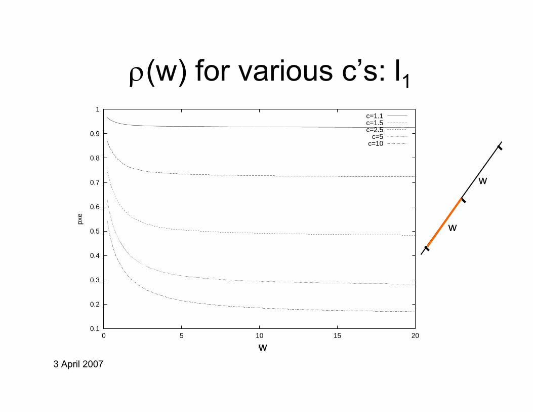
ρ(w) for various c’s: l1
0.1
0.2
0.3
0.4
0.5
0.6
0.7
0.8
0.9
1
0 5 10 15 20
pxe
r
c=1.1c=1.5c=2.5
c=5c=10
w
w
w

3 April 2007
ρ(w) for various c’s: l2
0
0.1
0.2
0.3
0.4
0.5
0.6
0.7
0.8
0.9
1
0 5 10 15 20
pxe
r
c=1.1c=1.5c=2.5
c=5c=10
w
w
w

3 April 2007
ρ(c) for l2
1 2 3 4 5 6 7 8 9 100
0.1
0.2
0.3
0.4
0.5
0.6
0.7
0.8
0.9
1
Approximation factor c
rho1/c

3 April 2007
New LSH scheme [Andoni-Indyk’06]
• Instead of projecting onto R1,project onto Rt , for constant t
• Intervals → lattice of balls– Can hit empty space, so hash until
a ball is hit• Analysis:
– ρ=1/c2 + O( log t / t1/2 )– Time to hash is tO(t)
– Total query time: dn1/c2+o(1)
• [Motwani-Naor-Panigrahy’06]: LSH in l2 must have ρ ≥ 0.45/c2
Xw
w
p
p

3 April 2007
New LSH scheme, ctd.• How does it work in practice ?• The time tO(t)dn1/c2+f(t) is not very
practical– Need t≈30 to see some improvement
• Idea: a different decomposition of Rt
– Replace random balls by Voronoidiagram of a lattice
– For specific lattices, finding a cell containing a point can be very fast →fast hashing
3 April 2007
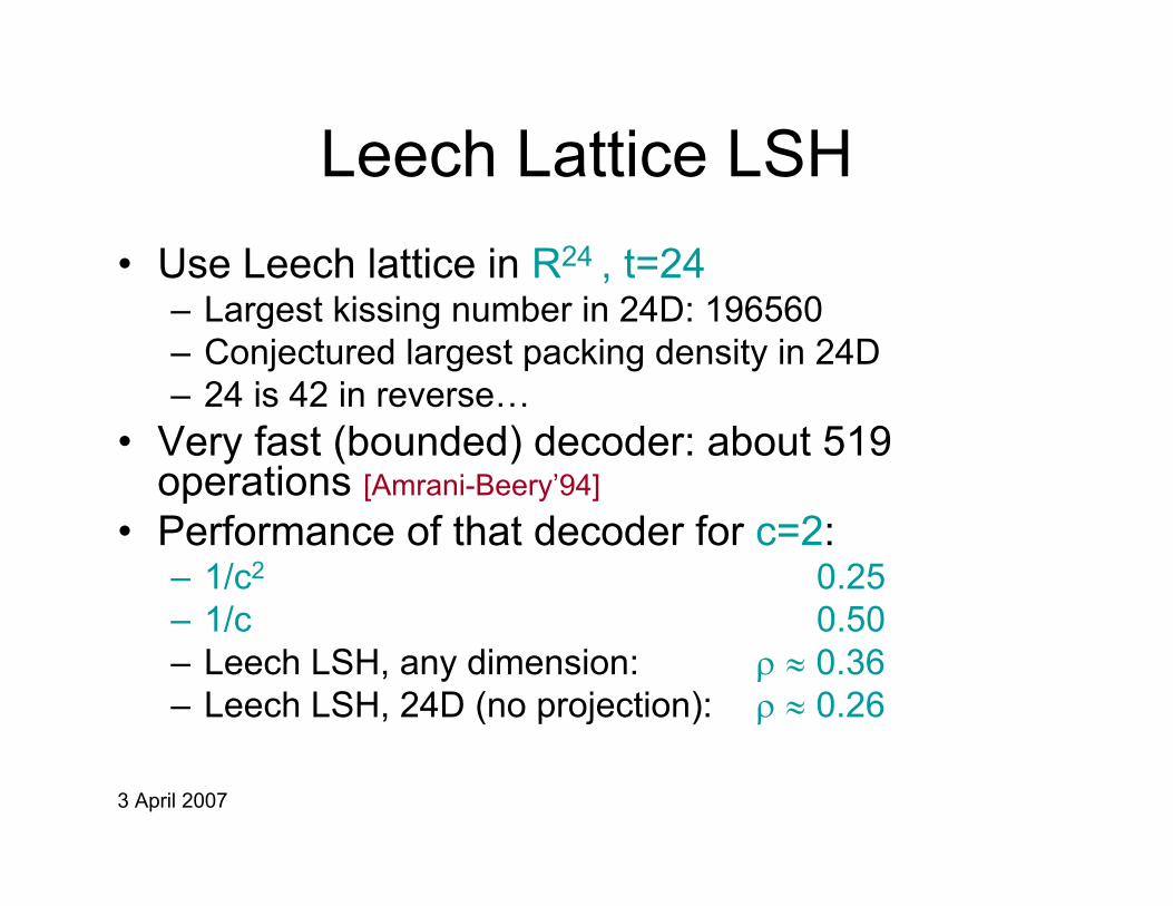
Leech Lattice LSH• Use Leech lattice in R24 , t=24
– Largest kissing number in 24D: 196560– Conjectured largest packing density in 24D– 24 is 42 in reverse…
• Very fast (bounded) decoder: about 519 operations [Amrani-Beery’94]
• Performance of that decoder for c=2:– 1/c2 0.25– 1/c 0.50– Leech LSH, any dimension: ρ ≈ 0.36– Leech LSH, 24D (no projection): ρ ≈ 0.26

3 April 2007
Experiments

3 April 2007
Experiments (with ’04 version)• E2LSH: Exact Euclidean LSH (with Alex Andoni)
– Near Neighbor– User sets r and P = probability of NOT reporting a point within
distance r (=10%)– Program finds parameters k,L,w so that:
• Probability of failure is at most P• Expected query time is minimized
• Nearest neighbor: set radius (radiae) to accommodate 90% queries (results for 98% are similar)– 1 radius: 90%– 2 radiae: 40%, 90%– 3 radiae: 40%, 65%, 90%– 4 radiae: 25%, 50%, 75%, 90%

3 April 2007
Data sets• MNIST OCR data, normalized (LeCun)
– d=784– n=60,000
• Corel_hist– d=64– n=20,000
• Corel_uci– d=64– n=68,040
• Aerial data (Manjunath)– d=60– n=275,476

3 April 2007
Other NN packages
• ANN (by Arya & Mount):– Based on kd-tree– Supports exact and approximate NN
• Metric trees (by Moore et al):– Splits along arbitrary directions (not just x,y,..)– Further optimizations
3 April 2007
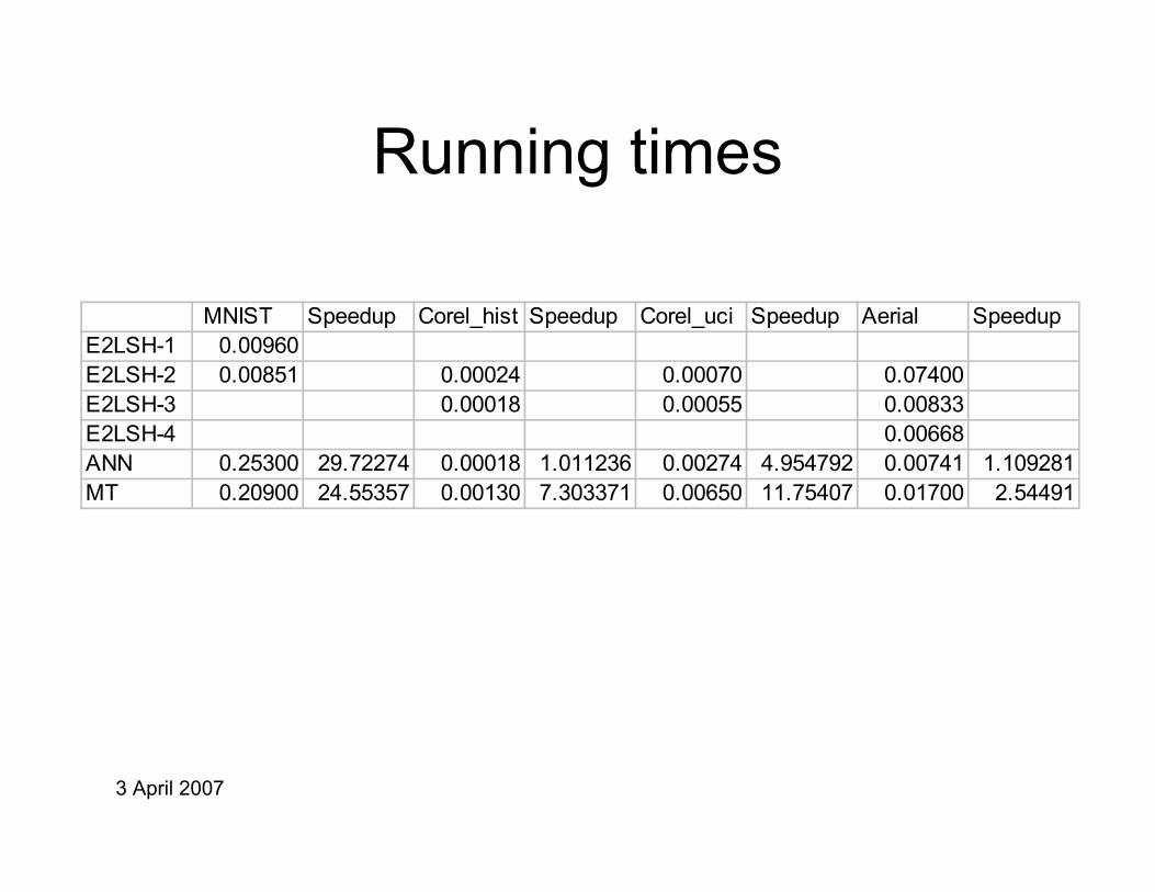
Running times
MNIST Speedup Corel_hist Speedup Corel_uci Speedup Aerial SpeedupE2LSH-1 0.00960 E2LSH-2 0.00851 0.00024 0.00070 0.07400E2LSH-3 0.00018 0.00055 0.00833E2LSH-4 0.00668ANN 0.25300 29.72274 0.00018 1.011236 0.00274 4.954792 0.00741 1.109281MT 0.20900 24.55357 0.00130 7.303371 0.00650 11.75407 0.01700 2.54491
3 April 2007
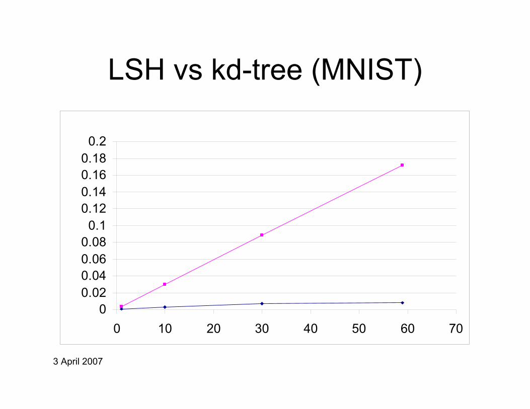
LSH vs kd-tree (MNIST)
00.020.040.060.08
0.10.120.140.160.18
0.2
0 10 20 30 40 50 60 70

3 April 2007
Caveats
• For ANN (MNIST), setting ε=1000% results in:– Query time comparable to LSH– Correct NN in about 65% cases, small error otherwise
• However, no guarantees• LSH eats much more space (for optimal
performance):– LSH: 1.2 GB– Kd-tree: 360 MB
3 April 2007
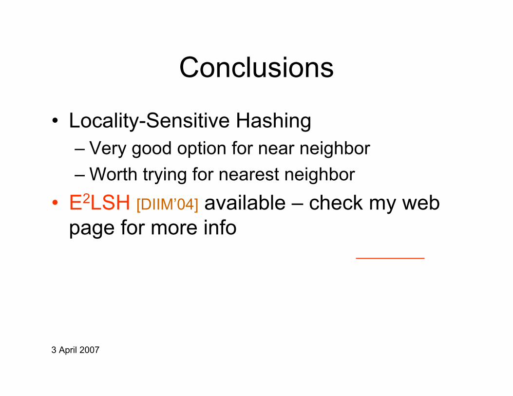
Conclusions
• Locality-Sensitive Hashing– Very good option for near neighbor– Worth trying for nearest neighbor
• E2LSH [DIIM’04] available – check my web page for more info