Approximation algorithms for some vehicle routing problems ∗

Cristina Bazgan † Refael Hassin ‡ Jerome Monnot †

Abstract

We study vehicle routing problems with constraints on the distance traveled byeach vehicle or on the number of vehicles. The objective is either to minimize thetotal distance traveled by vehicles or to minimize the number of vehicles used. Wedesign constant differential approximation algorithms for kVRP. Note that, using thedifferential bound for Metric 3VRP, we obtain the randomized standard ratio 197

99+

ε, ∀ε > 0. This is an improvement of the best-known bound of 2 given by Haimovich etal. [12]. For natural generalizations of this problem, called Edge Cost VRP, VertexCost VRP, Min Vehicle and kTSP we obtain constant differential approximationalgorithm and we show that these problems have no differential approximation scheme,unless P=NP.

Keywords: differential ratio, approximation algorithm, VRP, TSP

1 Introduction

Vehicle routing problems that involve the periodic collection and delivery of goods and ser-vices as mail delivery or trash collection are of great practical importance. Simple variantsof these real problems can be modeled naturally with graphs. Unfortunately even simplevariants of vehicle routing problems are NP -hard. In this paper we consider approximationalgorithms, and measure their efficiencies in two ways. One is the standard measure givingthe ratio apx

opt, where opt and apx are the values of an optimal and approximate solution, re-

spectively. The other measure is the differential measure, that compares the worst ratio of,on the one hand, the difference between the cost of the solution generated by the algorithmand the worst cost, and on the other hand, the difference between the optimal cost and theworst cost. Formally, the differential measure gives the ratio α = wor−apx

wor−opt, where wor is the

value of the optimal solution for the complementary problem. In [15], the measure 1 − α

is considered and it is called there z-approximation. Justification for this measure can befound for example in [1, 6, 27, 15, 20].

The main subject of this paper is differential approximation of routing problems. Inthese problems n customers have to be served by vehicles of limited capacity from a commondepot. A solution consists of a set of routes, where each starts at the depot and returnsthere after visiting a subset of customers, such that each customer is visited exactly once.We refer to a problem as a vehicle routing problem (VRP) if there is a constraint onthe (possibly weighted) number of customers visited by a vehicle. This constraint reflects

∗A preliminary shortened version has appeared in CIAC’03† LAMSADE, Universite Paris-Dauphine, Place du Marechal de Lattre de Tassigny, 75775 Paris Cedex

16, France. Email: {bazgan,monnot}@lamsade.dauphine.fr‡ Department of Statistics and Operations Research, Tel-Aviv University, Tel Aviv 69978, Israel. E-mail:

hassin@post.tau.ac.il

1

the assumption that the vehicle has a finite capacity and that it collects from the customers(or distributes among them) a commodity. The goal is to find a solution such that the totallength of the routes is as small as possible. In other cases, the vehicle is just supposedto visit the customers, for example, in order to serve them. In such cases we refer to theproblem as a TSP problem. We will assume in such cases that the limitation is on the totaldistance traveled by a vehicle and not on the number of customers it visits, and in this casewe search solution with a minimum number of vehicles used.

The problems that are considered here generalize the (undirected) Traveling Sales-man Problem (TSP). Differential approximation algorithms for the TSP are given byHassin and Khuller [15] and Monnot [20]. We will sometimes use these algorithms togenerate approximations for the problems of this paper. However, we note an importantdifference. In the TSP, adding a constant k to all of the edge length does not affect the setof optimal solutions or the value of the differential ratio. The reason is that every solutioncontains exactly n edges and therefore every solution value increases by exactly the samevalue, namely nk. In particular, this means that for the purpose of designing algorithmswith bounded differential ratio, it doesn’t matter whether d is a metric or not (it can bemade a metric by adding a suitable constant to the edge lengths). In contrast, in some ofproblems dealt with here, the number of edges used by a solution is not the same for everysolution and therefore it may turn out, as we will see, that in some cases the metric versionis easier to approximate.

It is easy to see that 2VRP is polynomial time solvable. For k ≥ 3, Metric kVRPwas proved NP -hard by Haimovich and Rinnooy Kan [11]. In [12], Haimovich, RinnooyKan and Stougie gave a 5

2 −32k

standard approximation for Metric kVRP. We study for thefirst time the differential approximability of kVRP. More exactly we give a 1

2 differentialapproximation for the non-metric case for any k ≥ 3. We improve this bound to 3

5 forMetric 4VRP and 2

3 for Metric kVRP with 5 ≤ k ≤ 8. We also improve the cases

k = 3 and k ≥ 9 to 5099 − ε, ∀ε > 0 and 25(k−1)

33k− ε, ∀ε > 0 respectively by using a random

algorithm. An approximation lower bound of 22192220 is given here for Metric nVRP with

length 1 and 2 using a lower bound of TSP(1,2) [8].

We study a generalization of VRP, called Edge Cost VRP, where the maximumlength traversed by each vehicle is bounded. We establish a 1

3 differential approximationfor this problem.

Min-Max kTSP is a generalization of TSP where we search to cover the customers byat most k vehicles such that the maximum length traversed by the vehicles is minimum.The metric case of the problem was studied by Fredrickson, Hecht and Kim [9] wherethey give a 5

2 − 1k

standard approximation algorithm by constructing a reduction fromthis problem to Metric TSP and using Christofides’ algorithm [4] . We establish a 1

2differential approximation for Metric Min-Max kTSP and prove that it has no differentialapproximation scheme. We also give a standard lower bound of p+1

pfor Min-Max ⌊n

p⌋TSP,

for p ≥ 6.

Min-Sum EkTSP is another generalization of TSP where we search to cover the cus-tomers by exactly k vehicles such that the total length is minimum. We show that MetricMin-Sum EkTSP is 2

3 differential approximable and it has no differential approximationscheme unless P=NP.

In Min vehicle the goal is to minimize the number of vehicles subject to a constraint onthe maximum length traversed by any single vehicle. In [19], Li, Simchi-Levi and Desrochersproved that Min Vehicle is not standard 2 approximable, unless P=NP and it is 1 + α

α−2

2

standard approximable where α = λdm

and dm = max{d0,1, . . . , d0,n}. We first present a23 differential approximation algorithm and show how to improve the bound to 289

360 . Wealso show that even when λ is constant and the lengths are 1 and 2, Min Vehicle has nostandard and differential approximation scheme, unless P=NP. We can improve the boundof 2

3 to 289360 .

The paper is organized as follows: In section 2 we give the necessary definitions. Insection 3 we give a constant differential approximation algorithm for General kVRP, anda better constant differential approximation for the metric case. In section 4 the main resultis a constant differential approximation for Edge Cost VRP. In the last three sections weshow that Min-Max kTSP, Min-Sum EkTSP and Metric Min Vehicle are constantdifferential approximable and have no differential approximation scheme, if P 6= NP.

2 Terminology

Given an instance x of an optimization problem and a feasible solution y of x, we denoteby val(x, y) the value of the solution y, by opt(x) the value of an optimal solution of x, andby wor(x) the value of a worst solution of x. The differential approximation ratio of y is

defined as δ(x, y) = |val(x,y)−wor(x)||opt(x)−wor(x)| . This ratio measures how the value of an approximate

solution val(x, y) is located in the interval between opt(x) and wor(x). In particular, it isequivalent for a minimization problem to prove δ(x, y) ≥ ε and val(x, y) ≤ εopt(x) + (1 −ε)wor(x).

For a function f , f(n) < 1, an algorithm is a f(n) differential approximation algorithmfor a problem Q if, for any instance x of Q, it returns a solution y such that δ(x, y) ≥ f(|x|).We say that an optimization problem is constant differential approximable if, for someconstant δ < 1, there exists a polynomial time δ differential approximation algorithm forit. An optimization problem has a differential polynomial time approximation scheme ifit has a polynomial time (1 − ε) differential approximation, for every constant ε > 0. Wesay that two optimization problems are standard (differential) equivalent if a δ differentialapproximation algorithm for one of them implies a δ standard (differential) approximationalgorithm for the other one.

We consider in this paper several routing problems. The problems are defined on acomplete undirected graph denoted G = (V, E). The vertex set V consists of a depot vertex0, and customer vertices {1, . . . n}, and each edge (i, j) ∈ E is endowed with a weightdi,j ≥ 0. We call a such graph a complete valued graph. We refer to the version of theproblem in which d is assumed to satisfy the triangle inequality as the metric case. Theoutput to the problems consists of a p-tour, that is, a set of simple cycles, C1, . . . , Cp, suchthat V (Ci)∩ V (Cj) = {0}, ∀i 6= j, and ∪p

i=1V (Ci) = V . The sequence (0, i, 0) with i 6= 0 isaccepted as a cycle. We now describe the problems. For each one we specify the input, theproblem’s constraints, and the output.

kVRPInput: A complete valued graph.Constraint: |Cj | ≤ k + 1, j = 1, . . . , p.Output: A p-tour minimizing the total weight of the cycles.

Edge Cost VRPInput: A complete valued graph and a metric {ℓi,j (i, j ∈ E}, and λ > 0.

3

Constraint:∑

e∈E(Cj) ℓe ≤ λ, j = 1, . . . , p.Output: A p-tour minimizing the total weight of the cycles.

Vertex Cost kVRPInput: A complete valued graph and a function {ci ≥ 0 i ∈ V }, where ci denotes the costof the vertex i.Constraint:

∑

i∈V (Cj) ci ≤ k, j = 1, . . . , p.Output: A p-tour minimizing the total weight of the cycles.

Min-Max kTSPInput: A complete valued graph.Constraint: p ≤ k.Output: A p-tour minimizing the maximum weight of the cycles.

Min-Sum EkTSPInput: A complete valued graph.Constraint: p = k.Output: A p-tour minimizing the total weight of the cycles.

Min VehicleInput: A complete valued graph and λ > 0.Constraint:

∑

e∈E(Cq) de ≤ λ, j = 1, . . . , p.Output: A p-tour minimizing p.

Min DistanceInput: A complete valued graph and λ > 0.Constraint:

∑

e∈E(Cq) de ≤ λ, j = 1, . . . , p.Output: A p-tour minimizing the total weight of the cycles.

For an optimization problem Q with edge lengths, we denote by Q(a, b) the version ofQ where weights are between a and b and more specifically Q[t], for t > 1, the variantwhere b ≤ ta for any a > 0. We will use the following problem:

Min TSP Path(1,2) is the variant of Min TSP(1,2) problem where instead of a tourwe ask for a Hamiltonian path of minimum weight. Min TSP Path(1,2) has no differentialapproximation scheme [22] even if opt = n − 1 and wor = 2(n − 1) where n is the numberof vertices since it is proved in [2] that Min TSP(1,2), when the subgraph restricted toedges of length 1 is Hamiltonian and cubic, has no standard approximation scheme.

We will also use the following problems:

partitioning into paths of length k (kPP): Given a graph G = (V, E) with |V | =(k + 1)q, is there a partition of V into q paths P1, . . . , Pq, each path with k + 1 vertices?2PP have been proved NP-complete in [10] whereas, more generally, the NP-completenessof kPP is proved in [18] as a special of G-partition problem. Thus (n − 1)PP is thedecision version of Hamiltonian Path.

Maximum weighted partitioning into paths with at most k vertices (Maxweighted atmostkPP): Given a weighted complete graph G where each edge (i, j) ∈ E isendowed with a weight di,j ≥ 0, we want to find a partition of vertices into paths P1, . . . , Pq,each path with at most k vertices (or indifferently k−1 edges) such that

∑qi=1 d(Pi) is max-

4

imum. There is an easy reduction proving the NP -hardness of this problem between kPPand Max weighted atmost(k + 1)PP that consist to complete the graph G instance ofkPP by edges of weight 0.

A binary 2-matching (also called 2-factor or cycle cover) is a subgraph in which eachvertex in V has a degree of exactly 2. Since the graph is simple, each cycle has at leastthree vertices. A minimum binary 2-matching is one with minimum total edge weight.Hartvigsen [14] has shown how to compute a minimum binary 2-matching in O(n3) time(see [25] for another O(n2|E|) algorithm). More generally, a binary f-matching, where f isa vector of size n + 1, is a subgraph in which each vertex i of V has a degree of exactly fi.A minimum binary f-matching is one with minimum total edge weight and is computablein polynomial time [5].

3 kVRP

nVRP is standard equivalent to TSP. So, using the result of Sahni and Gonzalez [26] wededuce that nVRP is not 2p(n) standard approximable for any polynomial p, unless P=NP.In fact for any k ≥ 5 the problem is as hard to approximate as nVRP.

Theorem 3.1 For all k ≥ 5 (even if k is a function of n), kVRP, is not 2p(n) standardapproximable for any polynomial p, unless P=NP.

Proof: We use a reduction from partitioning into paths of length k (kPP). Given thegraph G = (V, E) on n = (k+1)q vertices we construct a graph G′ instance of (k+3)VRP.We add a vertex 0 (the depot) to G and a set A of 2q vertices. We define the function d

as follows: di,j = 1, if i ∈ V ∪ {0} and j ∈ A or if (i, j) ∈ E and i, j ∈ V . Finally, theremaining edges have weight n2p(n).

If G contains a decomposition into disjoint paths of k+1 vertices then opt(G′) = q(k+4),otherwise opt(G′) > n2p(n). So, a 2p(n) standard approximation for (k+3)VRP could decidekPP in polynomial time. The conclusion follows.

3.1 General kVRP

When d is a metric, the reduction of TSP to nVRP is straightforward, and it easily followsthat computing opt is NP-hard. On the other hand, this reduction between the correspond-ing maximization problems Max TSP and Max nVRP leading to the conclusion thatcomputing wor is also NP-hard, does not work. We can easily prove this result by applyinga reduction from kPP with weight 1 and 3.

In the following we give a 12 differential approximation for non-metric kVRP.

We first compute a lower bound LB. Then we generate a feasible solution for G withvalue good = LB + δ1. Next, we generate another feasible solution of value bad = LB + δ2

where δ2 ≥ δ1. This proves that the approximate solution with value good is an α-differentialapproximation where

α =wor − good

wor − opt≥

bad − good

bad − opt≥

δ2 − δ1

bad − LB=

δ2 − δ1

δ2= 1 −

δ1

δ2, (1)

since for a minimization problem wor ≥ bad ≥ good ≥ opt ≥ LB. To generate LB wereplace 0 by a complete graph with a set V0 of 2n vertices and zero length edges. The

5

distance between a vertex of V0 and a vertex i of V \V0 is the same as the distance between0 and i. Denote the resulting graph by G′. Compute in G′ a minimum weight binary2-matching M ′.

Lemma 3.2 Let LB denote the weight of M ′, and denote by opt the value of an optimalVRP solution. Then opt ≥ LB.

Proof: It is sufficient to show that for any VRP solution in G there exists a binary 2-matching in G′ with the same value. Consider an optimal VRP solution in G and let C be acycle in it. Generate in G′ a cycle C ′ which is as C except for that 0 is replaced by two newadjacent vertices from V0. Repeat this process for every cycle in the VRP solution, takingcare that the subsets of vertices selected from V0 are disjoint (an optimal solution may onlycontain cycles (0, i, 0) for i = 1, . . . , n and in such a case, we need to use all vertices of V0).In the last cycle insert all the remaining vertices of V0. The result is a binary 2-matchingsince every cycle has at least three vertices and the cycles are disjoint and cover V . Sincethe value of cycle C ′ is the same as the value of C, the optimum of VRP is greater than orequal to the minimum binary 2-matching.

Lemma 3.3 A binary 2-matching M ′ of G′ can be transformed in polynomial time into aset M of cycles covering vertices of G with the same weight.

Proof: If a cycle of M ′ does not contain a vertex of V0 then this cycle is considered inM . If a cycle of M ′ contains more than one consecutive vertices from V0 then replace thesevertices by one vertex of V0. Consider in the following a cycle C ′ of M ′ containing at leastone vertex from V0 and one from V (G′)\V0. Suppose that C ′ = (v1

0, µ1, v20, µ2, . . . , v

t0, µt, v

10)

where paths µ1, . . . , µt contain only vertices from V (G′) \ V0. Then M will contain t cycles(0, µ1, 0), (0, µ2, 0), . . . , (0, µt, 0) that have the same weight as C ′.

We suggest the following algorithm. W.l.o.g. we suppose that the current cycle is(0, 1, . . . , m, 0).

Algo Differential VRP

1 Compute LB the weight of a minimum weight binary 2-matching M ′ in G′;

2 Transform M ′ into M = {C1, . . . , Cp}, using Lemma 3.3;

3 For every cycle Ci = (1, . . . , mi, 1) of M do

3.1 If mi ≡ 0 mod 2 then

3.1.1 soli,1 := {(0, 1, 2, 0), (0, 3, 4, 0), . . . , (0, mi − 1, mi, 0)};

3.1.2 soli,2 := {(0, mi, 1, 0), (0, 2, 3, 0), . . . , (0, mi − 2, mi − 1, 0)};

3.2 If mi ≡ 1 mod 2 then

3.2.1 soli,1 := {(0, 1, 2, 0), (0, 3, 4, 0), . . . , (0, mi − 4, mi − 3, 0)}∪{(0, mi − 2, mi − 1, mi, 0)};

3.2.2 soli,2 := {(0, mi, 1, 0), (0, 2, 3, 0), . . . , (0, mi − 3, mi − 2, 0)} ∪ {(0, mi − 1, 0)};

6

1

2

3

4

5

66

11

1

6

4

55

5

sol3sol2sol1C

4

62 2 2

4

333

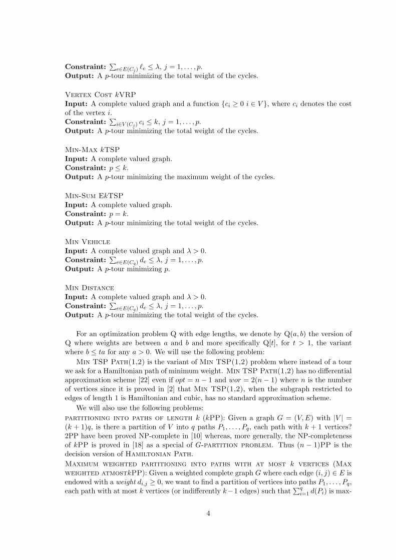
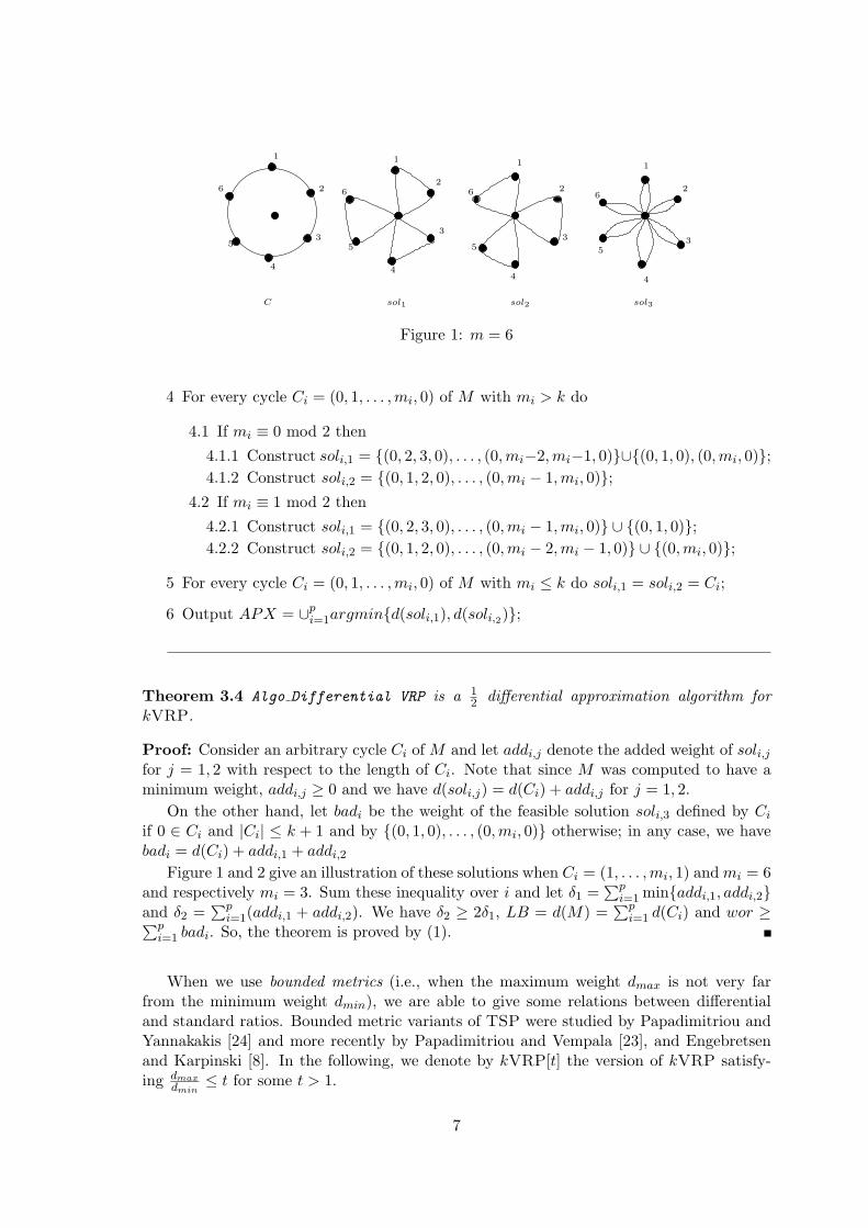
Figure 1: m = 6

4 For every cycle Ci = (0, 1, . . . , mi, 0) of M with mi > k do

4.1 If mi ≡ 0 mod 2 then

4.1.1 Construct soli,1 = {(0, 2, 3, 0), . . . , (0, mi−2, mi−1, 0)}∪{(0, 1, 0), (0, mi, 0)};

4.1.2 Construct soli,2 = {(0, 1, 2, 0), . . . , (0, mi − 1, mi, 0)};

4.2 If mi ≡ 1 mod 2 then

4.2.1 Construct soli,1 = {(0, 2, 3, 0), . . . , (0, mi − 1, mi, 0)} ∪ {(0, 1, 0)};

4.2.2 Construct soli,2 = {(0, 1, 2, 0), . . . , (0, mi − 2, mi − 1, 0)} ∪ {(0, mi, 0)};

5 For every cycle Ci = (0, 1, . . . , mi, 0) of M with mi ≤ k do soli,1 = soli,2 = Ci;

6 Output APX = ∪pi=1argmin{d(soli,1), d(soli,2)};

Theorem 3.4 Algo Differential VRP is a 12 differential approximation algorithm for

kVRP.

Proof: Consider an arbitrary cycle Ci of M and let addi,j denote the added weight of soli,jfor j = 1, 2 with respect to the length of Ci. Note that since M was computed to have aminimum weight, addi,j ≥ 0 and we have d(soli,j) = d(Ci) + addi,j for j = 1, 2.

On the other hand, let badi be the weight of the feasible solution soli,3 defined by Ci

if 0 ∈ Ci and |Ci| ≤ k + 1 and by {(0, 1, 0), . . . , (0, mi, 0)} otherwise; in any case, we havebadi = d(Ci) + addi,1 + addi,2

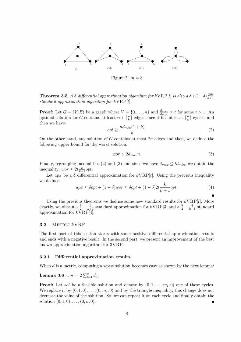
Figure 1 and 2 give an illustration of these solutions when Ci = (1, . . . , mi, 1) and mi = 6and respectively mi = 3. Sum these inequality over i and let δ1 =

∑pi=1 min{addi,1, addi,2}

and δ2 =∑p

i=1(addi,1 + addi,2). We have δ2 ≥ 2δ1, LB = d(M) =∑p

i=1 d(Ci) and wor ≥∑p

i=1 badi. So, the theorem is proved by (1).

When we use bounded metrics (i.e., when the maximum weight dmax is not very farfrom the minimum weight dmin), we are able to give some relations between differentialand standard ratios. Bounded metric variants of TSP were studied by Papadimitriou andYannakakis [24] and more recently by Papadimitriou and Vempala [23], and Engebretsenand Karpinski [8]. In the following, we denote by kVRP[t] the version of kVRP satisfy-ing dmax

dmin≤ t for some t > 1.

7

3

222

3

C sol1 sol2 sol3

13 111

Figure 2: m = 3

Theorem 3.5 A δ differential approximation algorithm for kVRP[t] is also a δ+(1−δ) 2tkk+1

standard approximation algorithm for kVRP[t].

Proof: Let G = (V, E) be a graph where V = {0, . . . , n} and dmax

dmin≤ t for some t > 1. An

optimal solution for G contains at least n + ⌈nk⌉ edges since it has at least ⌈n

k⌉ cycles, and

then we have:

opt ≥ndmin(1 + k)

k. (2)

On the other hand, any solution of G contains at most 2n edges and then, we deduce thefollowing upper bound for the worst solution:

wor ≤ 2dmaxn. (3)

Finally, regrouping inequalities (2) and (3) and since we have dmax ≤ tdmin, we obtain theinequality: wor ≤ 2t k

k+1opt.

Let apx be a δ differential approximation for kVRP[t]. Using the previous inequalitywe deduce:

apx ≤ δopt + (1 − δ)wor ≤ δopt + (1 − δ)2tk

k + 1opt. (4)

Using the previous theorems we deduce some new standard results for kVRP[t]. Moreexactly, we obtain a 7

2 −3

k+1 standard approximation for kVRP[3] and a 92 −

4k+1 standard

approximation for kVRP[4].

3.2 Metric kVRP

The first part of this section starts with some positive differential approximation resultsand ends with a negative result. In the second part, we present an improvement of the bestknown approximation algorithm for 3VRP.

3.2.1 Differential approximation results

When d is a metric, computing a worst solution becomes easy as shown by the next lemma:

Lemma 3.6 wor = 2∑n

i=1 d0,i

Proof: Let sol be a feasible solution and denote by (0, 1, . . . , mi, 0) one of these cycles.We replace it by (0, 1, 0), . . . , (0, mi, 0) and by the triangle inequality, this change does notdecrease the value of the solution. So, we can repeat it on each cycle and finally obtain thesolution (0, 1, 0), . . . , (0, n, 0).

8

In Theorem 3.4 we have shown that kVRP is 12 differential approximable. We now show

that in the metric case, the same bound can be achieved by a simpler algorithm.

We compute a minimum weight perfect matching M on the subgraph induced by{1, . . . , n}, if n is even, or by {0, 1, . . . , n} if n is odd. We link each endpoint differentof 0 of M to the depot. We claim that

opt ≥ 2d(M). (5)

Indeed, consider an optimum solution for kVRP. Walk around it and shortcut in orderto obtain a Hamiltonian cycle C on {0, 1, . . . , n} if n is odd and a Hamiltonian cycle C on{1, . . . , n} if n is even. We have opt ≥ d(C) by the triangle inequality and this cycle is thesum of two perfect matchings which are greater than or equal to M .

Using (5), Lemma 3.6 and the construction of the approximate solution, we obtain:

apx = d(M) +n

∑

i=1

d0,i ≤1

2opt +

1

2wor , (6)

proving that the result is a 12 differential approximation.

Theorem 3.7 Metric kVRP is δ·k−1k

differential approximable, where δ is the differentialapproximation ratio for Metric TSP.

Proof: Our algorithm modifies the Optimal Tour Partitioning heuristic of Haimovich,Rinnooy Kan and Stougie [12]: first construct a tour T of value val(T ) on V using the δ

differential approximation algorithm for TSP. W.l.o.g., assume that this tour is describedby the sequence (0, 1, . . . , n, 0). We produce k solutions soli for i = 1, . . . , k and we selectthe best solution. The first cycle of soli is formed by the sequence (0, 1, . . . , i, 0) and theneach other cycle (except possibly the last) of soli has exactly k consecutive vertices (forinstance, the second cycle is (0, i + 1, . . . , i + k, 0)) and finally, the last cycle is formed bythe unvisited vertices (connecting n to the depot 0). Denote by apxi for i = 1, . . . , k thevalues of the solution soli and by apx the value of the best one.

In the union of solutions sol1, . . . , solk each edge of T \ {(0, 1), (0, n)} appear exactly(k − 1) times and each edge (0, j) for j 6= 1, n appears exactly twice. Finally, edges (0, 1)and (0, n) appear exactly (k + 1) times. Since worV RP = 2

∑ni=1 d0,i by Lemma 3.6, we

deduce:

apx ≤1

k

k∑

i=1

apxi ≤(k − 1)

kval(T ) +

1

kworV RP . (7)

Since T is a δ differential approximation then

val(T ) ≤ (1 − δ)worTSP + δoptTSP . (8)

Since it is possible to construct from an optimum solution of VRP a solution of TSP witha smaller value (using the triangle inequality), it follows that

optTSP ≤ optV RP (9)

Also, by connecting the depot twice with each customer, we can construct from a solutionof TSP a solution of VRP with a greater value, and therefore

worTSP ≤ worV RP (10)

9

Using (7)-(10) we obtain that

apx ≤ δk − 1

koptV RP +

(

1 − δk − 1

k

)

worV RP .

Since the best known differential approximation algorithm for TSP is 23 [15, 20] then

the algorithm of Theorem 3.7 is an 23 · k−1

kdifferential approximation algorithm for metric

kVRP. For k > 4 this is an improvement over the bound of 12 given by Theorem 3.4 for

the general (non-metric) kVRP.

We will proceed now to improve the bound given in Theorem 3.7 by using a genericalgorithm. When we deal with a cycle of size m we consider the vertices modulo m.

Algo Differential MetrickVRP

1 Find a partition of V \ {0} by cycles M = {C1, . . . , Cp} using a Preprocessing

algorithm;

2 For every cycle Ci = (1, . . . , mi, 1) of M with mi = kq + r, 0 ≤ r < k do

2.1 For j = 1 to mi do

2.1.1 Let (µ1, . . . , µ⌈mik

⌉) = Ci\[{(j, j+1)}∪{(j+r+ℓk, j+r+1+ℓk) : 0 ≤ ℓ < q}];

2.1.2 Construct soli,j = ∪⌈

mik

⌉

ℓ=1 {(0, µℓ, 0)};

2.2 Let soli = argmin{d(soli,1), . . . , d(soli,mi)}

3 Output APX = ∪pi=1soli;

By using the construction of solutions soli,1, . . . , soli,mi, we easily deduce the following

lemma:

Lemma 3.8 Consider a cycle Ci = (1, . . . , mi, 1) of M with mi = kq + r, 0 ≤ r < k. Wehave:

(i)∑mi

j=1 d(soli,j) = (mi − q)d(Ci) + 2q∑mi

j=1 d(0, j) if r = 0.

(ii)∑mi

j=1 d(soli,j) = (mi − q − 1)d(Ci) + 2(q + 1)∑mi

j=1 d(0, j) if r 6= 0.

Proof:(i): soli,j contains ⌈mi

k⌉ = q cycles for every j = 1, . . . , mi. Thus, in ∪mi

j=1soli,j , eachedge of Ci appears exactly mi − q times and each edge (0, j) appears exactly 2q times.

(ii): soli,j contains ⌈mi

k⌉ = q + 1 cycles for every j = 1, . . . , mi. So, the same argument

as previously shows that each edge of Ci appears exactly mi − (q + 1) times and each edge(0, j) appears exactly 2(q + 1) times in ∪mi

j=1soli,j .

Theorem 3.9 Metric 4VRP is 35 differential approximable and Metric kVRP is 2

3differential approximable with 5 ≤ k ≤ 8.

10

Proof: Our preprocessing algorithm works as follows: we compute a minimum weightbinary 2-matching M = (C1, . . . , Cp) on the subgraph induced by V \{0}. Consider a cycleCi = (1, . . . , mi, 1) of M with mi = kq + r and let wori = 2

∑mi

j=1 d0,j .

Assume q = 0. Since the best solution (i.e., soli) is better than the average one, weobtain using Lemma 3.8:

d(soli) ≤r − 1

rd(Ci) +

1

rwori =

1

r(wori − d(Ci)) + d(Ci) . (11)

Since wori ≥ d(Ci) by the triangle inequality and r ≥ 3 (Ci contains at least 3 vertices),we deduce:

d(soli) ≤2

3d(Ci) +

1

3wori . (12)

Now, assume q ≥ 1. If r = 0, then we deduce:

d(soli) ≤k − 1

kd(Ci) +

1

kwori ≤

2

3d(Ci) +

1

3wori . (13)

since k ≥ 3. Otherwise, we have r ≥ 1 and we obtain:

d(soli) ≤q + 1

kq + r(wori − d(Ci)) + d(Ci)

and we deduce since r, q ≥ 1:

d(soli) ≤k − 1

k + 1d(Ci) +

2

k + 1wori (14)

On the one hand, it is possible to construct from an optimum solution of Metric VRPa feasible solution of TSP on the subgraph induced by V \ {0} (by shortcutting) with asmaller value and we deduce d(M) =

∑pi=1 d(Ci) ≤ optTSP ≤ optV RP . On the other hand

wor =∑q

i=1 wori. Finally, by summing over i the inequalities (12), (13) and (14) and bydistinguishing the case k = 4 and k > 4 we obtain the expected result.

The algorithm of Theorem 3.9 works for any k ≥ 3 and it gives the ratio 12 for Metric

3VRP and 23 for k ≥ 9. We now improve the previous bound for k = 3 and k ≥ 9 using

another preprocessing algorithm. But surprisingly, this algorithm compute an approximateTSP with maximum weight.

Observation 3.10 The differential and standard approximation ratios for Max weightedatmostkPP coincide. Indeed, we have wor = 0 since {Pi}i∈V where Pi = {i} is a feasiblesolution.

This problem is very close to Metric kVRP when we deal with differential ratio:

Theorem 3.11 For any k ≥ 3, Max weighted atmostkPP and Metric kVRP aredifferential equivalent.

Proof: In order to reduce Metric kVRP to Max weighted atmostkPP, consider aninstance G of Metric kVRP with n customers. We construct an instance I ′ of Maxweighted atmostkPP as follows: we delete the depot 0 and consider the graph Kn andset d′x,y = d0,x + d0,y − dx,y for any vertices x, y ∈ V \ {0}. By the triangle inequality,

11

d′x,y ≥ 0. d′x,y denotes the saving gained with respect to the worst solution, by joining x

and y in a cycle rather then reaching each of them from the depot. We have an one to onecorrespondence between a path P = (1, . . . , j) using at most k vertices in I ′ and the cycleC = (0, 1, . . . , j, 0) with at most k customers in G. Moreover, d′(P ) = 2

∑ji=1 d0,i − d(C).

Finally, we also have an one to one correspondence between feasible solutions of these twoproblems, and since wor = 2

∑ni=1 d0,i, for any solution of G of value val we have

val′ = worV RP − val. (15)

Conversely we reduce Max weighted atmostkPP to Metric kVRP. Let G and d

be an instance of Max weighted atmostkPP. We add a depot 0 and we set: d′0,i =maxe∈E de,∀i ∈ V and d′i,j = 2 maxe∈E de − di,j ,∀i, j ∈ V . The rest of the proof is similar.

Let ρ be the standard approximation ratio for Max TSP. The current best value for ρ

is 2533 obtained by a randomized algorithm in [17].

Theorem 3.12 Metric kVRP is (2533

k−1k

− ε) differential randomized approximable fork ≥ 3 and any ε > 0.

Proof: Let G be an instance of Metric kVRP with n customers and let ε > 0. In order toobtain a good solution for G, we apply algorithm Algo Differential MetrickVRP wherethe preprocessing is a tour T = C1. This tour is produced by the algorithm from [17]applied on the instance I ′ = (Kn, d′) with n = kq + r obtained from G as in Theorem 3.11,algorithm that is a 25

33 randomized approximation. Using the definition of weight d′ and theLemma 3.8, we obtain:

worV RP − apx = max1≤j≤n

d′(sol1,j) ≥

∑nj=1 d′(sol1,j)

n≥ (

k − 1

k− ε)d′(C1).

when q ≥ k−1εk2 − 1

k. Otherwise, we exhaustively solve the problem.

On the other hand, an optimal solution of Max weighted atmostkPP on I ′ can beused to construct a feasible solution of Max TSP on I ′ by joining the endpoints of the paths.Hence optMaxTSP ≥ optMax weighted atmostkPP. Finally, by using the 25

33 standard approxi-mation algorithm for Max TSP for obtaining the tour T , we have d′(C1) ≥

2533optMaxTSP

and optMax weighted atmostkPP = worV RP − optV RP since (15).

In particular, we obtain a (5099 − ε) differential randomized approximation for Metric

3VRP, that is better than the 12 differential approximation given in Theorem 3.4. It

also improves the result of Theorem 3.9 for k ≥ 9 since we obtain the differential ratioδ = 25(k−1)

33k− ε > 2

3 for Metric kVRP. For instance, this ratio is 200297 ≃ 0.67 for k = 9.

We summarize in the following the differential results that we obtain for Metric kVRP:

• Metric 3VRP is (5099 − ε) differential randomized approximable for any ε > 0.

• Metric 4VRP is 35 differential approximable.

• Metric kVRP is 23 differential approximable for 5 ≤ k ≤ 8.

• Metric kVRP is (2533

k−1k

− ε) differential randomized approximable for any k ≥ 9and for any ε > 0.

12

Finally, note the similarity between the results given in Theorem 3.7 and the one givenin Theorem 3.12. They both deal with the reduction in approximation from MetrickVRP to Max TSP (Max TSP and Min Metric TSP are equivalent with respect tothe differential ratio [20]) and the expansion is very similar δ k−1

kfor Theorem 3.7 and

ρk−1k

− ε for Theorem 3.12. The only difference is on the measure used: The first reductionconsiders the differential ratio for the two problems whereas the second one considers thestandard ratio for Max TSP. Actually, the standard ratio ρ = 25

33 is better than differentialratio δ = 2

3 for Max TSP and more generally the best standard ratio ρbest for Max TSPwill be always better than the best differential ratio δbest (i.e., ρbest ≥ δbest) since we have atrivial reduction from any maximization problem to itself transforming a differential resultinto a standard result (see Lemma 1.3 in Monnot [20]), leading to the conclusion that thereduction of Theorem 3.12 is better. Nevertheless, if the optimal result is ρbest = δbest thenthe reduction of Theorem 3.7 will be better.

Since nVRP and TSP are standard equivalent, from the result of Papadimitriou andYannakakis [24] we deduce immediately that nVRP(1,2) has no standard approximationscheme unless P = NP. Also TSP(1,2) has no differential approximation scheme [21] butwe cannot deduce immediately that nVRP(1,2) has no differential approximation schemesince wornV RP and worTSP may be very far. However, we prove in the following a lowerbound for the differential approximation of nVRP(1,2).

Theorem 3.13 nVRP(1, 2) is not (22192220 − ε) differential approximable, for any constant

ε > 0, unless P=NP.

Proof: Since wornV RP ≤ 4n ≤ 4optnV RP , a δ differential approximation for nVRP(1, 2)gives a δ+4(1−δ) standard approximation for nVRP(1, 2). Using the negative result givenin [8] that TSP(1,2) is not 741

740 − ε standard approximable, we obtain the expected result.

3.2.2 Some standard approximation results

Despite these observations, by using Theorem 3.9 for Metric kVRP and Theorem 3.5 weestablish better standard approximation ratio than Haimovich, Rinnooy Kan and Stougie(i.e., (5

2 − 32k

) standard approximation) when we deal with bounded metrics, i.e., dmax ≤tdmin. More exactly, Metric 4VRP[2] is 47

25 standard approximable and Metric kVRP[2]is (2 − 4

3(k+1)) standard approximable for k ≥ 5.

We now describe some results concerning the standard approximability of MetrickVRP. In [12], a (5

2 − 32k

) standard approximation for Metric kVRP is obtained byreduction to Metric TSP and using Christofides’ algorithm.

The following theorem gives a reduction preserving the approximation scheme betweenstandard and differential ratio even if we deal with unbounded metrics (dmax

dminis not upper

bounded).

Theorem 3.14 A δ differential approximation algorithm for Metric kVRP is also ak − δ(k − 1) standard approximation algorithm.

13

Proof: Consider an optimal solution for an instance G of Metric kVRP and w.l.o.g.denote by (0, 1, . . . , mi, 0) one of its cycles. Using the triangle inequality, the length of thiscycle is at least 2max{d0,i : i = 1, . . . , mi} ≥ 2

k

∑mi

i=1 d0,i. Summing over each cycle, weobtain using Lemma 3.6:

opt ≥2

k

n∑

i=1

d0,i =wor

k. (16)

Let apx be a δ differential approximation for G. Using the inequality (16) we deduce:

apx ≤ δopt + (1 − δ)wor ≤ δopt + k(1 − δ)opt. (17)

Using Theorem 3.14, Observation 3.10 and Theorem 3.12 we obtain:

Corollary 3.15 Metric 3VRP is (3− 43ρ+ ε) standard approximable for all ε > 0 where

δ is the standard approximation ratio for Max TSP.

More exactly, since ρ = 2533 [17] we obtain the bound 197

99 ≃ 1.99 that is an improvementof the 2 standard approximation of Haimovich et al. [12].

4 Edge Cost VRP

We assume now that each edge is associated with a cost ℓ satisfying the triangle inequality,and the solution must satisfy that the total cost on each cycle does not exceed λ.

Note that if we do not assume that ℓ is a metric then even deciding whether the problemhas any feasible solution is NP-complete. For a proof see Theorem 7.1 below. Therefore,we assume that ℓ satisfies the triangle inequality, and to ensure feasibility we also assumethat 2ℓ0,i ≤ λ for i = 1, . . . , n.

Theorem 4.1 Edge Cost VRP is 13 differential approximable.

Proof: We start with a binary 2-matching as described in Lemma 3.2 except that theinitial graph is not a complete undirected graph G but a partial graph G′ of it built bydeleting the edges (i, j) for i 6= 0 and j 6= 0 such that ℓ0,i + ℓi,j + ℓj,0 > λ. Observe thatM is still a lower bound of an optimal solution of Edge Cost VRP. Then, we applythe algorithm Algo Differential VRP except that we change steps 3.2, 5 and 6. Thestep 3.2 becomes the following: we produce mi solutions soli,1, . . . , soli,mi

where soli,j ={(0, j + 1, j + 2, 0), . . . , (0, j − 2, j − 1, 0)} ∪ {(0, j, 0)} for j = 1, . . . , mi.

The step 5 becomes: for every cycle Ci = (0, 1, . . . , mi, 0) of M with∑

e∈E(Ci) ℓe ≤ λ dosoli,1 = soli,2 = Ci whereas the step 6 becomes: the solution APX is the solution obtainedby concatenating the shortest of soli,j for each cycle Ci.

Observe that in step 3.2, each edge of Ci appears exactly ⌊mi

2 ⌋ times in (∪j≤misoli,j)

and each edge (0, j) appears exactly mi +1 times. Thus, since mi ≥ 2, the same argumentsas in Theorem 3.4 proved that APX is a 1

3 differential approximation.

In [12], the authors consider two versions of kVRP with additional constraint on thelength of each cycles. In the first problem that we will call here Vertex Cost kVRP, eachcustomer has a cost and we want to find a solution such that the total customer cost on

14

each cycle does not exceed k. In the second, called in [19] Min metric Distance, we wantto find a solution such that the total cost on each cycle does not exceed a given bound λ.For each of these two problems, we give a differential reduction preserving approximationscheme from Edge Cost VRP.

Lemma 4.2 A δ differential approximation solution for Edge Cost VRP (respectively,metric case) is also a δ differential approximation for Vertex Cost kVRP (respectively,metric case).

Proof: Let G = (V, E) with d and c be an instance of Vertex Cost kVRP. We constructan instance of Edge Cost VRP as follows. First we set λ = k. The graph and the functiond are the same whereas the function ℓ is defined by: ℓi,j =

ci+cj

2 where we assume thatc0 = 0. This function satisfies the triangle inequality. Moreover, let C be a cycle linkingthe depot to a subset of customers. We have

∑

i∈V (C) ci ≤ λ iff∑

e∈E(C) ℓe ≤ λ.

Corollary 4.3 Vertex Cost kVRP is 13 differential approximable.

Min Metric Distance is a particular case of Edge Cost VRP where the function ℓ

is exactly the function d. Thus, from Theorem 4.1 we deduce the corollary:

Corollary 4.4 Min Metric Distance is 13 differential approximable.

For Edge Cost VRP and Vertex Cost kVRP there have neither standard nordifferential approximation scheme unless P = NP since these two problems contain nVRP.

5 Min-Max kTSP

The metric case of the problem was studied by Fredrickson, Hecht and Kim [9] wherethey give a 5

2 − 1k

standard approximation algorithm by constructing a reduction from thisproblem to Metric TSP and using Christofides’ algorithm [4].

Theorem 5.1 Min-Max rTSP is not 2p(n) standard approximable for any polynomial p

and r ≥ 1, unless P=NP.

Proof: We reduce Hamiltonian Path problem to Min-Max rTSP. We start with thereduction described in Theorem 3.1 with k = n − 1 and q = 1 and the weight n2p(n) isreplaced by (n + 3)2p(n) (recall that the (n − 1)PP problem is the Hamiltonian Pathproblem) and we apply r times this reduction (so, the final graph consists of depot and r

copies of G and set A of 2r vertices). Thus, a 2p(n) standard approximation for Min-MaxrTSP could decide Hamiltonian Path, that is proved NP-hard in [10].

We now turn to the metric case. We give a 12 differential approximation algorithm for

Metric Min-Max kTSP, k ≥ 2 and we show that the problem has neither standard nordifferential approximation scheme unless P=NP.

Theorem 5.2 Metric Min-Max 2TSP is 12 differential approximable.

15

Proof: Consider a tour T = (0, . . . , n, 0) of G. Let i be the smallest index such that∑i

j=0 dj,j+1 ≥ d(T )2 . We consider the solution C1 = (0, 1, . . . , i, 0) and C2 = (0, i + 1, . . . , n, 0).

Note that

d(C1) − d0,i =i−1∑

j=0

dj,j+1 ≤d(T )

2

and

d(C2) − d0,i+1 = d(T ) −i

∑

j=0

dj,j+1 ≤ d(T ) −d(T )

2=

d(T )

2.

So, max{d(C1), d(C2)} ≤ d(T )2 + max{d0,i, d0,i+1} ≤ worTSP

2 + opt2TSP

2 . Since a worsttour on V with the value worTSP is a feasible solution for 2TSP then wor2TSP ≥ worTSP .Thus, max{d(C1), d(C2)} ≤ wor2TSP

2 + opt2TSP

2 .

Corollary 5.3 Metric Min-Max kTSP is 12 differential approximable.

Proof: The previous algorithm is a 12 differential approximationfor general k ≥ 3 since we

have also workTSP ≥ worTSP and max{d0,i, d0,i+1} ≤ optkTSP

2 .

Theorem 5.4 Min-Max kTSP(1,2), k ≥ 2 has neither standard nor differential polyno-mial time approximation scheme, unless P=NP.

Proof: We construct a L-reduction from Min TSP(1,2), when the subgraph restricted tothe edges of length 1 is Hamiltonian, to Metric Min-Max kTSP.

Let G be a complete graph on n vertices, with edges of length 1 and 2. We construct aninstance G′ of Min-Max kTSP adding to G a depot, the vertex 0, and we set the distancebetween 0 and a vertex i of G to 2. Suppose that n = q · k + r, 0 < r ≤ k. It is easyto see that opt(G) = optTSP (G) = n and opt(G′) = optMin−Max kTSP (G′) = q + 4 sincethe optimum of G′ is obtained when the Hamiltonian cycle is divided in k paths where thedifference of sizes is at most 1. So opt(G′) = opt(G)−r

k+ 4, or opt(G) = k · opt(G′) − 4k + r.

From a solution of G′ with value val′ we construct a solution in G putting together thepaths induced by the solution in G and linking these paths by edges of length at most 2.This solution has the value val ≤ k(val′ − 4) + 2k. So,

val−opt(G) ≤ k ·val′−2k−k ·opt(G′)−4k + r ≤ k[val′−opt(G′)]−5k ≤ k[val′−opt(G′)].

Since Min TSP(1,2), when the subgraph restricted to edges of length 1 is Hamiltonian,has no standard polynomial time approximation scheme [2], then Min-Max kTSP also hasno standard approximation scheme.

In order to see that Min-Max kTSP has no differential approximation scheme, we showthat if it was the case then Min-Max kTSP on the particular instances that we considerabove would have a standard approximation scheme. Suppose that Min-Max kTSP hasa differential approximation scheme Aδ, ∀δ, 0 < δ < 1. So, Aδ gives a solution for G′ witha value val ≤ δopt(G′) + (1 − δ)wor(G′). For the above instances G′ of Min-Max kTSP,opt(G′) = n−r

k+4 and wor(G′) = 2(n−1)+4 ≤ 2kopt(G′). Thus, val ≤ [δ+2k(1−δ)]opt(G′),

and for an (1 + ε) standard approximation solution for an instance of Min-Max kTSP,∀ε > 0, we apply Aδ with δ = 1 − ε

2k−1 .

For certain cases we can give inapproximability gaps, for examples, when we have ⌊n6 ⌋

vehicles we can prove that the problem is not 76 approximable and more generally we obtain:

16

Theorem 5.5 Min-Max ⌊nk⌋TSP(1,2), k ≥ 6 is not k+1

k− ε standard approximable for

any ε > 0, unless P=NP.

Proof: We use a reduction from (k − 4)PP with k ≥ 6. We use the reduction described inTheorem 3.1 except that we replace the distances n2p(n) by distances 2. Then, if G containsa decomposition in paths of length k − 4 then opt(G′) = k, otherwise opt(G′) ≥ k + 1. So,a k+1

k− ε standard approximation for Min-Max ⌊n

k⌋TSP(1,2) could decide (k − 4)PP in

polynomial time.

6 Min-Sum EkTSP

Bellmore and Hong [3] showed that when the constraint p = k is replaced by p ≤ k, thenMin-Sum kTSP is standard equivalent to TSP on an extended graph. This is true evenfor the directed version of the problem and when there is a cost associated with activatinga salesman. For our case the transformation simply involves replacing the depot vertex 0by k vertices of zero distance. Also, the metric case of the p ≤ k version is not of interestsince the solution is just a single cycle (thus, we deal with the case p = k and Min-SumEkTSP denote this problem).

Min-Sum EkTSP is differential equivalent to Metric Min-Sum EkTSP. This obser-vation follows since the number of edges in every solution is the same (like in the TSPcase). Hence, we add a constant to all the edge lengths and achieve the triangle inequalitywithout affecting the best and worst solutions.

Similarly, Min-Sum EkTSP is differential equivalent to Max-Sum EkTSP.

Theorem 5.1 can be adapted in order to prove that Min-Sum EkTSP is not 2p(n)

standard approximable, for any polynomial p, unless P=NP.

We now give the main results of this section.

Theorem 6.1 Metric Min-Sum EkTSP is 23 differential approximable, ∀k ≥ 1.

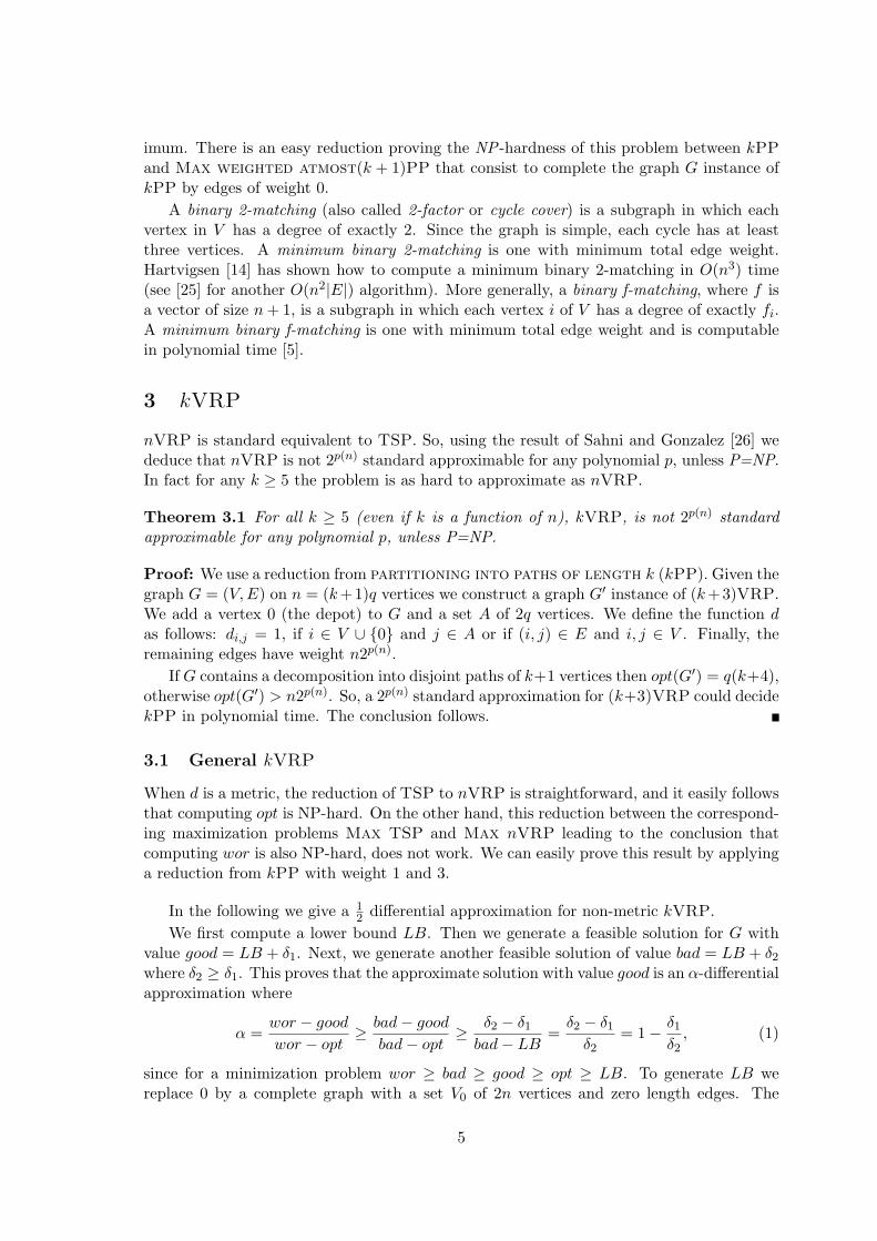
Proof: Let G and d be an instance of Metric Min-Sum EkTSP. Add to every edgeincident with the depot a parallel copy. Compute a minimum binary f -matching M ={C1, . . . , Cp} (C1, . . . , Ck denote the cycles of M containing the depot 0) on G where f(0) =2k and f(v) = 2 for v ∈ V \ {0}. Compute by using a 2

3 differential approximationalgorithm of [15] or [20] a solution C ′ for TSP on the subgraph G′ of G induced by V ′ =V \ (∪k−1

i=1 V (Ci)) ∪ {0}. The approximate solution sol for Metric Min-Sum EkTSPis composed of C ′ and the cycles C1, . . . , Ck−1. See Figure 3. Since M is a minimumbinary f -matching M on G then M ′ = M \ (∪k−1

i=1 Ci) is an optimum binary 2-matchingon G′. Let r =

∑k−1i=1 d(Ci). It is proved in [15] or [20] that the TSP algorithm gives a

solution satisfying val ≤ 23d(M ′)+ 1

3worTSP (G′). Since workTSP (G) ≥ worTSP (G′)+r andoptkTSP (G) ≥ d(M ′) + r, we deduce that the value of sol satisfies:

apx = val + r ≤2

3[d(M ′) + r] +

1

3[worTSP (G′) + r] ≤

2

3optkTSP (G) +

1

3workTSP (G)

Theorem 6.2 Unless P=NP, Min-Sum EkTSP(1,2) has no standard and differential ap-proximation scheme for any k ≥ 2.

17

C1

Ck−1

C1

Ck−1Ck

C′

0 0

Msol

V ′

Figure 3: M and sol

Proof: We reduce Min TSP Path (1,2) on Hamiltonian cubic graphs to Min-SumE2TSP(1,2). From a graph G = (V, E) on n vertices, we construct a graph G′ instanceof Min-Sum E2TSP(1,2). G′ consists of two copies of G and a vertex 0 (the depot).Within a copy, the edges have the same distance as in G; d0,i = 1, for each vertex i in oneof the two copies; di,j = 2 if i and j are vertices in different copies. Using the equalities

opt(G) = n−1 = wor(G)2 and opt(G′) = 2n+2, wor(G′) = 4n, we have opt(G′) = 2opt(G)+4

and wor(G′) = 2wor(G) + 4. Given a solution S of G′ with two cycles, we can transformit in another one S′ that contains exactly two cycles (0, P1, 0), (0, P2, 0), each of these twopaths are contained in a copy of G and with a better value. The idea for doing this is toremove the edges between the two copies in the solution S and in each copy, we arbitrarilyconnect the resulting paths. We consider as solution for G the path with the smallest value

among the two. So, val = min{val(P1), val(P2)} ≤ val(P1)+val(P2)2 = val(S′)−4

2 ≤ val(S)−42 .

Since opt(G) = opt(G′)2 − 2 and wor(G) = wor(G′)

2 − 2 then a δ differential approximationof Min-Sum E2TSP(1,2) gives a δ differential approximation for Min TSP Path (1,2)on Hamiltonian and cubic graphs. The conclusion follows for Min-Sum E2TSP(1,2) sinceMin TSP Path (1,2) on Hamiltonian and cubic graphs has no differential approximationscheme ([2, 22]). It is easy to see that if S is a (1 + ε

2) standard approximation of Min-Sum E2TSP(1,2) then the same solution as above with value val is a (1 + ε) standardapproximation of Min TSP Path (1,2). The proof for k ≥ 3 is similar.

7 Min Vehicle

In this problem, the goal is to visit the customers by a minimum number of vehicles, undera constraint on the total distance traveled by a vehicle.

In [19], it is proved that Metric Min Vehicle is not standard 2 approximable, unlessP=NP. Indeed even deciding whether the problem has a feasible solution is NP-complete:

Theorem 7.1 Deciding the feasibility of Min Vehicle is NP-complete.

Proof: In order to prove the NP-hardness, we reduce Hamiltonian Path problem to

18

Min Vehicle. We again apply the reduction described in Theorem 3.1 with k = n−1 andq = 1, except that the distances n2p(n) are replaced by the distances λ. Trivially there is afeasible solution for G′ only if λ ≥ n + 3. It is easy to see that Min Vehicle has a feasiblesolution iff G contains a Hamiltonian path.

In contrast, deciding the feasibility of Metric Min Vehicle is trivial, and the conditionsimply amounts to d(0, i) ≤ λ

2 for i = 1, . . . , n. The following theorem gives a positive resultfor this problem:

Theorem 7.2 Metric Min Vehicle is 23 differential approximable.

Proof: Consider the collection C of sets of vertices of feasible cycles (cycles that includethe depot and whose length is at most λ). Since we assume that d is a metric, C is amonotone collection, that is, if C ′ ⊂ C and C ∈ C then also C ′ ∈ C. This means that if G′

is a subgraph of G that includes the depot, then the optimal solution on G′ is at most thatof G. This allows us to apply the following “greedy” approach:

Construct feasible cycles with the depot and three vertices, as long as this is possible.Let G′ be the graph G except the vertices of these cycles (the depot is preserved in G′).For an edge (i, j), if d0,i + d0,j + di,j > λ then we remove this edge from G′. Denote theresulting graph also by G′. Find a maximum size matching in G′. We will show below thata such maximum size matching in G′ is an optimum solution on G′. We now show that theunion of these cycles is a 2

3 differential approximation.

Denote by k3 the number of cycles on three vertices and the depot, constructed in thefirst step of the algorithm. Denote by k2 (and k1) the number of edges (and isolated vertices)obtained in G′ when we search a maximum size matching. So, val(G) = k1 + k2 + k3.The value of the solution obtained in G′ in this way is val′ = k1 + k2 = |V (G′)| − k2

since k1 + 2k2 = |V (G′)|. Since we want to minimize val′ a maximum size matching givesan optimum solution. Since opt(G) ≥ opt(G′) and wor = n = |V (G)|, we obtain thatval(G) = k1 + k2 + k3 = k1 + k2 + n−k1−2k2

3 ≤ 23opt(G) + 1

3wor(G).

The algorithm of Theorem 7.2 is similar to the approach in [16] for obtaining differentialapproximation for Graph Coloring. By applying approximation algorithms for 3-SetCover and following the ideas of Halldorsson [13] for obtaining better differential approx-imation for Graph Coloring (see also [15]), the bound can be improved. Consider thefollowing algorithm: Construct feasible cycles with four vertices as long as this is possible.Let G′ be the graph G except the vertices of these cycles. List all the feasible cycles inG′. Note that such cycles include the depot and at most three other vertices, and thereforetheir number is polynomial. Apply an approximation algorithm for Min 3-Set ExactCover of a Monotone Collection, such as the algorithm of Halldorsson [13] or Duhand Furer [7]. This former result is a 3

4 -differential approximation (see Theorem 5.2 in [13]),and the latter gives a bound of 289

360 (see Theorem 4.2 in [7]). Note that the mentioned resultswere developed to give differential approximations for Graph Coloring, but they applyas well to any problem of exact covering by sets that correspond to a monotone collection(see Section 4 of [15]).

In [19], it is proved that unless P=NP, Min Vehicle is not standard 2 approximable andthus without standard approximation scheme when λ → ∞. In the following we establishthe same result for λ constant and for the differential case.

19

Theorem 7.3 Min Vehicle(1,2) has no standard and differential approximation schemeeven if λ is constant, unless P=NP.

Proof: We prove firstly that Min Vehicle(1,2) has no standard approximation scheme,if P 6= NP by reducing Min TSP(1,2) problem on Hamiltonian graphs to Min Vehi-cle(1,2). Min TSP(1,2) problem on cubic Hamiltonian graphs has no standard approxi-mation scheme [2], thus there is a constant ε0, 0 < ε0 < 1, such that it is not 1+ ε standardapproximable for ε ≤ ε0, if P 6= NP.

Given a graph G = (V, E) on n vertices, we construct a graph G′ instance of MinVehicle. G′ consists of one copy of G and a vertex 0 (the depot) and we define thefunction d′ as follows: d′0,i = 1, for i ∈ {1, . . . , n} and d′i,j = di,j if i, j ∈ {1, . . . , n}. It iseasy to see that opt1 = opt(G) = n and opt2 = opt(G′) = ⌈ n

λ−1⌉ ≤ nλ−1 + 1 ≤ n

λ−2 whenn ≥ (λ − 1)(λ − 2). Given a solution S′ of G′ with val2 vehicles, S′ = C1, . . . , Cval2 , weconsider as solution S for G the restriction of this solution to the vertices of G. The valueof S is val1 ≤

∑val2i=1 d(Ci) ≤ λval2 by the triangle inequality.

Suppose that Min Vehicle(1,2) would have a standard approximation scheme Aδ.We prove that this assumption imply that Min TSP(1,2) has an approximation scheme,contradiction. In order to obtain an (1 + ε) approximation for G, we apply A ε

3

on G′ with

λ = 3 + ⌈3ε⌉. Thus

val1 ≤ λ(1 +ε

3)

n

λ − 2≤ (1 + ε)n

since λ ≥ 3 + 3ε.

Using this last result we prove that this problem has no differential approximationscheme if P=NP. Suppose that Min Vehicle(1,2) when the graph restricted to edges ofweight 1 is Hamiltonian would have a differential δ approximation scheme Aδ, ∀δ, 0 < δ < 1.Therefore, for each instance G of the problem on n vertices, with λ = 3 + ⌈ 3

ε0⌉, this

algorithm gives a solution for G with a value val(G) ≤ δopt(G) + (1 − δ)wor(G). Sinceon these instances wor(G) = n and opt(G) = ⌈ n

λ−1⌉ ≥ nλ−1 then wor(G) ≤ (2 + 3

ε0)opt(G)

and so val(G) ≤ [δ + (2 + 3ε0

)(1 − δ)]opt(G). Thus, in order to obtain a standard (1 + ε)approximation algorithm, 0 < ε < 1, we have to take the solution given by Aδ withδ = 1 − ε ε0

3+ε0. The result follows since as we prove above Min Vehicle(1,2) on these

instances has no standard approximation scheme, unless P=NP.

References

[1] G. Ausiello, A. D’Atri and M. Protasi, “Structure preserving reductions amongconvex optimization problems,” Journal of Computing and System Sciences21(1980) 136-153.

[2] C. Bazgan, Approximation of optimization problems and total function of NP,Ph.D. Thesis (in French), Universite Paris Sud (1998).

[3] M. Bellmore and S. Hong, “Transformation of Multi-salesmen Problem to theStandard Traveling Salesman Problem,” Journal of the Association for ComputingMachinery 21(1974) 500-504.

[4] N. Christofides, “ Worst-case analysis of a new heuristic for the traveling salesmanproblem”, Technical report 338, Grad. School of Industrial Administration, CMU,1976.

20

[5] W.J. Cook, W.H. Cunningham, W.R. Pulleyblank, and A. Schrijver CombinatorialOptimization John Wiley & Sons Inc New York 1998 (Chapter 5.5).

[6] M. Demange and V. Paschos, “On an approximation measure founded on thelinks between optimization and polynomial approximation theory,” TheoreticalComputer Science 158(1996) 117-141.

[7] R-c. Duh and M. Furer, “Approximation of k-set cover by semi-local optimiza-tion,” Proc. of the Twenty Ninth Annual ACM Symposium on Theory of Comput-ing, 1996 256-264.

[8] L. Engebretsen and M. Karpinski, “Approximation hardness of TSP with boundedmetrics,” http://www.nada.kth.se/∼enge/papers/BoundedTSP.pdf

[9] G. N. Fredrickson, M. S. Hecht and C. E. Kim, “Approximation algorithms forsome routing problems,” SIAM J. on Computing 7(1978) 178-193.

[10] M. R. Garey and D. S. Johnson, “Computers and intractability. A guide to thetheory of NP-completeness,” Freeman, C.A. San Francisco (1979).

[11] M. Haimovich and A. H. G. Rinnooy Kan, “Bounds and heuristics for capacitatedrouting problems,” Mathematics of Operations Research 10(1985) 527-542.

[12] M. Haimovich, A. H. G. Rinnooy Kan and L. Stougie, “ Analysis of Heuristicsfor Vehicle Routing Problems,” in Vehicle Routing Methods and Studies, Golden,Assad editors, Elsevier (1988) 47-61.

[13] M.M. Halldorsson, “Approximating k-set cover and complementary graph color-ing,” Proc. of the 5th Conf. on Integer Programming and Combinatorial Optimiza-tion 1996, 118-131.

[14] D. Hartvigsen, Extensions of Matching Theory. Ph.D. Thesis, Carnegie-MellonUniversity (1984).

[15] R. Hassin and S. Khuller, “z-approximations,” Journal of Algorithms 41(2001)429-442.

[16] R. Hassin and S. Lahav, “Maximizing the number of unused colors in the vertexcoloring problem,” Information Processing Letters 52(1994) 87-90.

[17] R. Hassin and S. Rubinstein, “Better approximations for max TSP”, InformationProcessing Letters 75(2000) 181-186.

[18] D. G. Kirkpatrick and P. Hell, “On the completeness of a generalized matchingproblem,” Proc. of the 10th ACM Symposium on Theory and Computing (1978)240-245.

[19] C-L. Li, D. Simchi-Levi and M. Desrochers, “On the distance constrained vehiclerouting problem,” Operations Research 40(1992) 790-799.

[20] J. Monnot, “Differential approximation results for the traveling salesman andrelated problems,” Information Processing Letters 82(2002) 229-235.

21

[21] J. Monnot, V. Th. Paschos and S. Toulouse, “ Differential Approximation Resultsfor the Traveling Salesman Problem with Distances 1 and 2,” Proc. FCT (2001)275-286.

[22] J. Monnot, “The maximum Hamiltonian path problem with specified end-point(s),” Technical report Cahier du LAMSADE 176(2001).

[23] C. Papadimitriou and S. Vempala, “ On the approximability of the traveling sales-man problem ,” Proc. of the 32nd ACM Symposium on Theory and Computing(2000) 126-133.

[24] C. Papadimitriou and M. Yannakakis, “The traveling salesman problem with dis-tances one and two,” Mathematics of Operations Research 18(1993) 1-11.

[25] J. F. Pekny and D. L. Miller, “A staged primal-dual algorithm for finding a mini-mum cost perfect two-matching in an undirected graph,” ORSA Journal on Com-puting 6(1994) 68-81.

[26] S. Sahni and T. Gonzalez,“P-complete approximation problems” Journal of theAssociation for Computing Machinery 23(1976) 555-565.

[27] E. Zemel, “Measuring the quality of approximate solution to zero-one program-ming problems,” Mathematics of Operations Research 6(1981) 319-332.

22