approximation capabilities of wasserstein generative

Approximation Capabilities of WassersteinGenerative Adversarial Networks

Yihang GaoDepartment of Mathematics

The University of Hong KongHong Kong

[email protected]

Mingjie ZhouDepartment of Mathematics


[email protected]

Michael K. NgDepartment of Mathematics


[email protected]

Abstract

In this paper, we study Wasserstein Generative Adversarial Networks (WGANs) us-ing GroupSort neural networks as discriminators. We show that the error bound forthe approximation of target distribution depends on both the width/depth (capacity)of generators and discriminators, as well as the number of samples in training. Aquantified generalization bound is established for Wasserstein distance betweenthe generated distribution and the target distribution. According to our theoreticalresults, WGANs have higher requirement for the capacity of discriminators thanthat of generators, which is consistent with some existing theories. More impor-tantly, overly deep and wide (high capacity) generators may cause worse results(after training) than low capacity generators if discriminators are not strong enough.Numerical results on the synthetic data (swiss roll) and MNIST data confirm ourtheoretical results, and demonstrate that the performance by using GroupSort neuralnetworks as discriminators is better than that of the original WGAN.

1 Introduction

Generative Adversarial Networks (GANs), first proposed by Goodfellow et al. [17], have becomepopular in recent years for their remarkable abilities to approximate various kinds of distributions,e.g., common probability distributions in statistics, distributions of pixels in images [17, 31], and evenfor the natural language generation [8]. Several variants of GANs achieve much better performancesnot only in generation quality [3, 28, 20, 32, 37] but also in training stability [3, 34, 9] and efficiency[24, 22]. For more details about GANs, please refer to some latest reviews [18, 10, 16, 1].

Although empirical results have shown the success of GANs, theoretical understandings of GANsare still not sufficient. Even if the discriminator is fooled and the generator wins the game intraining, we usually cannot answer whether the generated distribution D is close enough to thetarget distribution Dtarget. Arora [4] found that if the discriminator is not strong enough (with fixedarchitecture and some constraints on parameters), the generated distribution D can be far away fromthe target distribution Dtarget, even though the learning has great generalization properties. Basedon the theoretical non-convergence of GANs (with constrained generators and discriminators), Baiet al. [5] designed some special discriminators with restricted approximability to let the trainedgenerator approximate the target distribution in statistical metrics, i.e., Wasserstein distance. However,their design of discriminators are not applicable enough because it can only be applied to some

arX

iv:2

103.

1006

0v2

[cs

.LG

] 2

6 M

ay 2

021

specific statistical distributions (e.g., Gaussian distributions and exponential families) and invertibleor injective neural networks generators. Liang [23] proposed a kind of oracle inequality to develop thegeneralization error of GANs’ learning in TV distance. However, several assumptions are requiredand KL divergence must be adopted to measure the distance between distributions. It may beinappropriate in generalization (convergence) analysis of GANs because many distributions in naturalcases lie on low dimensional manifolds. The support of the generated distribution must coincide wellwith that of the target distribution, otherwise, the KL divergence between these two are infinite, whichmay be not helpful in generalization analysis. After all, error bounds are usually much more strictthan empirical errors. Liang [23] showed the effectiveness of GANs in approximating probabilitydistributions to some extent.

Neural networks has been proved to have extraordinary expressive power. Two-layer neural networkswith sufficiently large width can approximate any continuous function on compact sets [19, 11, 27].Deep neural networks with unconstrained number of width and depth are capable of approximatingwider ranges of functions [40, 41]. After the wide applications and researches of deep generativemodel, e.g. VAEs and GANs, researchers began to study the capacity of deep generative networks forapproximating distributions. Yang et al. [39] recently proved that neural networks with sufficientlylarge width and depth can generate a distribution that is arbitrarily close to a high-dimensional targetdistribution in Wasserstein distances, by inputting only a one-dimensional source distribution (it leadsto the same conclusion for multi-dimensional source distribution).

Although deep generative networks have capacities to approximate distributions, discriminatorsplay an especially important role in GANs. If the discriminator is not strong enough (e.g. ReLUneural networks with limited architectures and constrained parameters), it can easily be fooled by thegenerator with even imperfect parameters. Both empirical and theoretical results show that GroupSortNeural Networks [35, 2] can approximate any 1-Lipschitz function arbitrary close in a compact setwith large enough width and depth. Therefore, in our generalization analysis of Wasserstein GAN,we adopt GroupSort Neural Networks as discriminators.

Motivated by the above mentioned research works, in this paper, we study the approximation fordistributions by Wasserstein GAN. Our contributions are given as follows.

(i) We connect the capacity of deep generative networks and GroupSort networks and derive ageneralization bound for Wasserstein GAN with finite samples. It implies that with sufficient trainingsamples, the Wasserstein GAN with proper choice of width and depth can approximate distributionswell. To the best of our knowledge, this is the first paper deriving the generalization bound inWasserstein distance of Wasserstein GAN in terms of the depth/width of the generators (ReLU deepneural networks) and discriminators (GroupSort Neural Networks), as well as the number of bothgenerated and real samples in training.

(ii) We analyse the importance for both generators and discriminators in WGANs. WGANs havehigher requirement for the capability of discriminators than that of generators according to ourderived generalization bound. We show that for nonparametric discriminators (discriminators arestrong enough), the generalization is easier to be obtained while the GroupSort neural networks (asdiscriminators) suffer a lot in the curse of dimensionality.

(iii) With the growing capacity (width and depth) of generators, width and depth of discriminatorsshould also be increased. Otherwise, the error will be augmented because of the large difference be-tween generators from the same generator class. In other words, overly deep and wide (high capacity)generators may cause worse results (after training) than low capacity generators if discriminators arenot strong enough.

Although generative models have potential risks, e.g. generating fake information, no further riskis created by our work which provides theoretical guidance and guarantee to the convergence ofthe previously proposed WGANs. Moreover, there exist some works on deep-fake detection [36].Therefore, the negative impacts produced by our work are limited.

The outline of the paper is given as follows. In Section 2, we give notations and mathematicalpreliminaries. In Section 3, we study generalization analysis for Wasserstein GAN and show theabove mentioned theoretical results. Numerical experiments are displayed in Section 4 to furtherverify our theoretical results. Finally, some concluding remarks are given in Section 5.

2

2 Notations and Preliminaries

2.1 Notations

Throughout the paper, we use ν, π and µθ to denote the target distribution, the source distribution (asan input to the generator) and the generated distribution (with θ as the parameters of the generator)respectively. More concretely, µθ is the distribution of gθ(Z), Z ∼ π, where gθ is a generator.The source distribution π lies on Rr, and both the target and the generated distribution are definedon Rd, where r and d are the number of dimensions. In Section 3, we use m for the number ofgenerated samples from µθ (the same number for samples from the source distribution π) and nfor the number of real data from the target distribution ν. The symbol . is used to hide someunimportant constant factors. For two functions `, h of a number n, ` . h means limn→+∞ `/h ≤ Cfor a non-negative constant C. For two positive real numbers or functions A and B, the term A ∨Bis equivalent to max{A,B} while A ∧ B is equivalent to min{A,B}. For V = (Vi,j) a matrixof size p × q, we let ||V||∞ = sup||x||∞=1 ||Vx||∞. We may also use the (2,∞) norm of V , i.e.||V||2,∞ = sup||x||2=1 ||Vx||∞.

2.2 Preliminaries

Different from the original model in [17], Generative Adversarial Networks (GANs) can be formulatedin a more general form:

mingθ∈G

maxf∈F

EZ∼πf(gθ(Z))− EX∈νf(X) (1)

where G is the generator class and F is the discriminator class. Here we assume that our pre-defineddiscriminator class is symmetric, i.e. f ∈ F and −f ∈ F . The symmetry condition is easy to besatisfied, e.g., feed-forward neural networks without activation functions in the last layer. Intuitively,the capacity of generator class G determines the upper bound for the quality of generated distributionsand the discriminator class F improves learning, pushing the learned parameters close to the optimalone. In practise, we can only access finite samples of target distribution; besides, only finite generateddata is considered due to limited computing power.. Empirically, instead of dealing with (1), weneed to solve the following adversarial problem and obtain the estimated (learned) parameters of thegenerator:

θm,n = mingθ∈G

maxf∈F{EmZ∼πf(gθ(Z))− EnX∼νf(X)} (2)

where EmZ∼π (respectively EnX∼ν) denotes the expectation on the empirical distribution of m (resp.n) i.i.d. samples of random variables Z (resp. X) from π (resp. ν). Therefore, the learned generatorgθm,n is obtained from (2).

Suppose that we have the following generator class G:

G = {gθ = NN(Wg, Dg, θ) : ‖Wi‖2 ≤M, ||bi||2 ≤M, 1 ≤ i ≤ Dg, θ = {W, b}} (3)

where NN(Wg, Dg, θ) denotes Neural Networks with Dg layers (depth), Wg neurons in each layer(width), and θ is the set of parameters. We useWi to represent the matrix of linear transform between(i− 1)-th and i-th layer. Here, we adopt ReLU as the activation function σ. The architecture of theneural networks is formulated as

NN(Wg, Dg,W) =WDg ◦ σ(WDg−1 ◦ σ(· · · ◦ σ(W1x+ b1) + · · · ) + bDg−1) + bDg

For Wasserstein GANs [3], the discriminator class FW is

FW = {f : ||f ||Lip ≤ 1} (4)

where ||f ||Lip is the Lipschitz constant of f . In section 3.1, we use FW as the discriminator class.However, the discriminator class FW is empirically impractical. In practice, several strategies areadopted to approximate FW in Wasserstein GANs. In this paper, we choose GroupSort neuralnetworks [2, 35] as the discriminator class. A GroupSort neural network is defined as

GS(Wf , Df , α) = VDf ◦ σk(VDf−1 ◦ σk(· · · ◦ σk(V1x+ c1) + · · · ) + cDf−1) + cDf (5)

where α = {V, c} denotes parameters of the GroupSort neural network, Wf is the width of eachlayer, Df is the depth (number of layers) and σk is the GroupSort activation function with groupingsize k. In the paper, k = 2. The Discriminator class is defined as

FGS = {fα = GS(Wf , Df , α) : GS(Wf , Df , α) is a Neural Network of form (5)} (6)

3

For more kinds of generator and discriminator classes, please refer to [22, 29, 30, 33].

Several kinds of probability metrics are available to measure the distance between two distributions.Empirical and theoretical results show their great performances [15, 21, 14, 25]. It has been statedabove that KL divergence and JS divergence (a special case of KL divergence) are not suitable forgeneralization (convergence) analysis of GANs due to the low dimensional properties of distributionsas well as the non-generalization property [3]. Wasserstein distance is a more relaxed and flexiblemetric and can generalize with some mild conditions (3-Moment of the distribution is finite). In ouranalysis, we adopt Wasserstein-1 distance (W1) as the evaluation metric between the generated andthe target distributions. The Wasserstein-p Distance (p ≥ 1) between two distributions µ and ν isdefined as

Wp(µ, ν) = infγ∈Γ(µ,ν)

∫||x− y||pd(γ(x, y))

where Γ(µ, ν) denotes the set of all joint distributions γ(x, y) whose marginals are µ and ν respec-tively. When p = 1, Kantorovich-Rubinstein duality [38] gives an alternative definition of W1:

W1(µ, ν) = sup||f ||Lip≤1

|EX∼µf(X)− EX∼νf(X)| = sup||f ||Lip≤1

EX∼µf(X)− EX∼νf(X). (7)

The last equation holds because of the symmetry (||f ||Lip = || − f ||Lip).

The remaining part studies how well the trained generator (obtained from (2)) is, with respect to itsWasserstein-1 distance to the target distribution ν (i.e. W1(µθm,n , ν)) for pre-defined generator classG and discriminator class F .

3 Generalization Analysis for Wasserstein GAN

3.1 Nonparametric Discriminators

In this subsection, we let the discriminator class F in (2) to be FW (defined in (4)) and the estimatedgenerator gθm,n is obtained from (2). Combining with Lemma 2, the following assumption guaranteesthat with sufficiently many samples, the empirical distributions ν and π are close (convergent) to νand π in W1 distance, respectively. The convergence requirements for both the source and the targetdistributions are essential because they are the base for GANs. If their empirical distributions are notconvergent, let alone distributions from learned generators.Assumption 1. Both the d dimensional target distribution ν and the r dimensional source distributionπ have finite 3-Moment, i.e. M3(ν) = EX∼ν |X|3 <∞ and M3(π) = EZ∼π|Z|3 <∞.Theorem 1 (Generalization of Wasserstein GAN with nonparametric discriminators). Suppose thatAssumption 1 holds for the target distribution ν (lies on Rd) and the source distribution π (lies onRr). For GANs, the generator class G is defined in (3) and the discriminator class F = FW (definedin (4)), i.e., the Wasserstein GAN. Let the learned parameters θm,n be obtained from (2), then thefollowing holds,

EW1(µθm,n , ν) ≤ mingθ∈G

W1(µθ, ν)+C1·MDg ·

m−1/2, r = 1m−1/2 logm, r = 2m−1/r, r ≥ 3

+C2·

n−1/2, d = 1n−1/2 log n, d = 2n−1/d, d ≥ 3

(8)where constants C1 and C2 are independent of M , Dg , Wg , m and n.

Proof of Theorem 1 can be found in Appendix A.1.Lemma 1 (Capacity of deep generative networks to approximate distributions [39]). Let p ∈ [1,∞)and π be an absolutely continuous probability distribution on R. Assume that the target distributionν is on Rd with finite absolute q-moment Mq(ν) <∞ for some q > p. Suppose that Wg ≥ 7d+ 1and Dg ≥ 2. Then there exists a neural network gθ = NN(Wg, Dg, θ) such that the generateddistribution µθ of gθ(Z), Z ∼ π has the following property:

Wp (µθ, ν) ≤ C(Mqq (ν) + 1

)1/p{ (W 2gDg

)−1/d, q > p+ p/d(

W 2gDg

)−1/d (log2W

2gDg

)1/d, p < q ≤ p+ p/d

where C is a constant depending only on p, q and d.

4

Remark. Although Lemma 1 holds for 1-dimensional source distribution, the result can be eas-ily generalized to high dimensional absolutely continuous source distributions simply by linearprojections.

Based on Lemma 1, we set p = 1 and q = 3, the generative net can transform the source distributionπ to a distribution that are arbitrary close to the target distribution ν. That means letting Wg , Dg andM be large enough, mingθ∈GW1(µθ, ν) can be arbitrarily small, i.e., with sufficiently large Wg , Dg

and M ,mingθ∈G

W1(µθ, ν) ≈ 0

With the fixed generator class G (Wg , Dg and M are fixed), letting m and n large enough, by (8) wehave

EW1(µθm,n , ν) ≈ mingθ∈G

W1(µθ, ν) ≈ 0

Because W1(µθm,n , ν) ≥ 0, we deduce that

W1(µθm,n , ν) ≈ 0, for most of the cases.

Lemma 1 provides an upper bound estimation for mingθ∈GW1(µθ, ν), however, for a concretebound of EW1(µθm,n , ν), we need further assumptions because the generator class in Lemma 1 isnot bounded. However, for a fixed target distribution ν and source distribution π, it’s reasonable toassume that Lemma 1 holds for the generator class with bounded parameters and fixed number oflayers (||W||2 ≤ M for sufficient large M and Dg is fixed but Wg is also bounded by M ). In thefollowing Assumption 2, we constrain the upper bound of Wg because wider matrix can have largeroperation norm.Assumption 2. For fixed target distribution ν and source distribution π, generator class G is definedin (3). Suppose that there exists a fixed depth Dg (Dg ≥ 2), and let M be large enough that for all7d+ 1 ≤Wg ≤M1/2, the bound of W1(µθ, ν) in Lemma 1 holds, i.e.

mingθ∈G

W1(µθ, ν) ≤ C ·W−2/dg D−1/d

g (9)

where C depends on M3(ν) and d.Remark. As we can see that ||W||2 usually grows with increasing width (i.e. Wg), that’s why webound Wg by M1/2. The assumption can be revised to other similar forms, as long as Wg is boundedby a monotonically increasing function of M . For large enough m, we assume that the Assumption 2holds for some M ≤ m1/(3rDg).Theorem 2 (Generalization bound for Wasserstein GAN with nonparametric discriminators). Sup-pose that Assumption 1 holds for the target distribution ν (lies on Rd) and the source distribution π(lies on Rr) respectively. For GANs, the generator class G is defined in (3) and the discriminator classF = FW (defined in (4)), i.e., the Wasserstein GAN. Further assume that Assumption 2 holds for thegenerators with fixed depthDg (Dg ≥ 2), large enoughM ≤ m1/(3rDg), and 7d+1 ≤Wg ≤M1/2.Let the parameters θm,n be obtained from (2), then the following holds,

EW1(µθm,n , ν) ≤ C·W−2/dg D−1/d

g +C1·m1/3r·

m−1/2, r = 1m−1/2 logm, r = 2m−1/r, r ≥ 3

+C2·

n−1/2, d = 1n−1/2 log n, d = 2n−1/d, d ≥ 3

(10)for large enough m and n, where constant C depends on M3(ν) and d; constant C1 depends onM3(π) and d; and constant C2 depends on M3(ν) and d.

Proof. Based on the above Theorem 1 and Assumption 2, (10) can be easily obtained.

3.2 Parametric Discriminators (GroupSort Neural Networks)

It is impractical to use FW as the discriminator class F . According to one of the approximationstrategies, we adopt GroupSort neural networks as discriminator class, i.e. F = FGS . The followingAssumption 3 guarantees that all the GroupSort Neural Networks in FGS are 1-Lipschitz becauseGroupSort activation function preserves norms.

5

Assumption 3. For all α =(V1, . . . ,VDf , c1, . . . , cDf

),

‖V1‖2,∞ 6 1 and max(‖V2‖∞ , . . . ,

∥∥VDf∥∥∞) 6 1

Assumption 4 (Decaying condition). Suppose that for a large enough number M satisfying M &M2Dg and M ≥ 2Dg ·MDg , and for s ≥ 3, there exists a constant C such that

P(||gθ(Z)||2 ≥ M

)≤ C · M−s and P

(‖X‖2 ≥ M

)≤ C · M−s

hold for X ∼ ν and all gθ ∈ G with Z ∼ π.

Remark. One of the reasons we bound the parameters of generator class are for the above decayingcondition (Assumption 4). For example, if the source distribution Z ∼ π is standard GaussianN (0, Ir) (one of the most accepted source distributions in GANs), then for all gθ ∈ G (which is MDg

Lipschitz), gθ(Z) is sub-Gaussian. To be more concrete, for any gθ ∈ G, we have

||gθ(Z)||2 ≤MDg ||Z||2 +Dg ·MDg

therefore,

P(||gθ(Z)||2 ≥ M

)≤ P

(||Z||2 ≥M−Dg (M −Dg ·MDg )

)≤ P

(||Z||2 ≥

1

2M−DgM

)When M & M2Dg and Z is from standard Gaussian distribution, then there exists a universalconstant C such that

P(||Z||2 ≥

1

2M−DgM

)≤ C · M−s

because P(||Z||2 ≥ M

)≤ C ′ · exp(−M2/2r). Any bounded distribution (i.e. values of samples

are bounded almost everywhere) apparently satisfies the above assumption. Moreover, with thedecaying condition, Assumption 1 for the finite 3-moment of ν is automatically satisfied.

Theorem 3 (Generalization bound for Wasserstein GAN with parametric discriminators). Supposethat Assumption 1 holds for the target distribution ν (lies on Rd) and the source distribution π(lies on Rr) respectively. For GANs, the generator class G is defined in (3) and the discriminatorclass F = FGS (defined in (6) and satisfying Assumption 3), i.e., the parametric Wasserstein GAN(GroupSort Neural Networks as discriminators). Further assume that Assumption 2 holds for thegenerators with fixed depth Dg (Dg ≥ 2), large enough M . m1/(3rDg) and 7d+ 1 ≤Wg ≤M1/2.Assumption 4 holds for some s ≥ 3 and M & M2Dg ≥ 2Dg ·MDg . Let the learned parametersθm,n be obtained from (2), then the following holds,

EW1(µθm,n , ν) . W−2/dg D−1/d

g + (m−1/6 logm ∨m−2/(3r)) + (n−1/2 log n ∨ n−1/d)

+ (2−Df/(2Cd2) ∨W−1/(2d2)

f ) +D−(s−1)f ∨W−(s−1)/(2d2)

f

(11)

when m, n, Df and Wf are sufficiently large, Df ≤ 2Df/(2Cd2) and M2Dg . M = W

1/(2d2)f ∧Df .

Here, . hides the parameters w.r.t d, r and some universal constants. C is a universal constant.

Remark. For detailed proof, please see Appendix A.2. The first term in the right hand side of(11) represents the error from the generator class. If we fix the number of layers and let the boundof parameters be large enough, then the capacity of generators improves with increasing width(with Assumption 2). The second term is the generalization error of generators with only finitenumber of samples. As we can see this term is actually related to the diversity of generators (aboutM and Dg), that’s why we constrain the number of layers and bound the parameters. The thirdterm is generalization error from the target distribution due to the limited number of observeddata. And the last two terms come from the approximation of GroupSort Neural Networks to 1-Lipschitz functions. The error is small if the width and depth of discriminators are large enough (theerror decays exponentially and polynomially with depth and width, respectively), which implies thecapacity and ability of Neural Networks. Noted that M2Dg . M = W

1/2d2

f ∧ Df shows severecurse of dimensionality in Wasserstein GAN’s error bound and it also means that GANs requirestrong discriminators, consistent with some famous empirical and theoretical results. Moreover,

6

Wg ≤M1/2 and M2Dg . M = W1/2d2

f ∧Df also indicate strict requirement for discriminators inGANs. It implies that overly deep and wide (high capacity) generators may cause worse results thanlow capacity generators if discriminators are not strong enough. Based on this, we have reasons tobelieve that the mode collapse in GANs may attribute to low capacity of discriminator class. Themain difference between Theorem 2 and Theorem 3 is the error from the approximation of FGS to1-Lipschitz functions.

Remark. Liang [23] derived a generalization bound for the generated distribution and the targetdistribution in TV distance. The main idea (oracle inequalities) is somewhat similar to our analysis.However, the bound involves KL divergence, which may be infinite if two distributions do not coincideon nonzero measure. Moreover, the pair regularization in his paper requires specially designedarchitectures of discriminators which may not widely applicable. After all, error bounds are usuallymuch more strict than empirical results. The results from Liang show the effectiveness of GANs inapproximating probability distributions to some extent.

4 Experimental Results

Our theoretical analysis in Section 3 conveys that with sufficient training data as well as the properchoice of depth and width of generators and discriminators, WGAN can approximate target distri-butions in Wasserstein-1 distance. In this section, both synthetic (Swiss roll) and actual (MNIST)datasets are utilized to verify our theoretical results. Although we derive the upper bound forW1(µθm,n , ν), numerical experiments confirm the consistence between the upper bounds and theactual Wasserstein-1 distances, at least in the trend.

The estimated Wasserstein distances between the target distributions and the generated distributionsare computed by POT package [13] on 10,000 samples. For each experiment, we repeat six timesand calculate the averaged Wasserstein distance to represent the expected value. For computationalefficiency, mini-batch SGD is adopted rather than updating on the whole dataset. Moreover, wegenerate noise at each iteration step because of its availability and cheapness. The features of ourinterest are the number of training data (denoted as n, consistent with those in theoretical analysis), aswell as width (Wg and Wf , respectively) and depth (Dg and Df , respectively) of both the generatorand the discriminator. A relaxed (proximal) constraints on the parameters are adopted [2, 35].Similarly, we use the Bjorck orthonormalization method to constrain parameters to be unit in || · ||2norm. For more details of Bjorck orthonormalization, please refer to [7, 2].

4.1 Synthetic Dataset (Swiss Roll)

To show the approximation of WGAN to data lying on low dimensional manifolds, we adopt the2-dimensional swiss roll (lies on an 1-dimensional manifold) as synthetic data in this subsection.Swiss roll curve are sampled from (x, y) ∼ (z · cos(4πz), z · sin(4πz)); z ∼ Uniform([0.25, 1]).

0.5 0.0 0.5 1.0

0.5

0.0

0.5 realgenerated

(a) 1000 training data0.5 0.0 0.5 1.0

0.5

0.0

0.5 realgenerated

(b) 6000 training data0 1000 2000 3000 4000 5000 6000

0.025

0.050

0.075

0.100

0.125

0.150

0.175

W1 d

istan

ce

GroupSort WGANsReLU WGANs

(c) number of training data

Figure 1: (GroupSort Neural Network as a Discriminator) Visualized real data and generated datawith (a) 1000 and (b) 6000 samples for training respectively; (c) The W1 distance between thegenerated distribution and the real distribution with different numbers of training data. Both thegenerator and the discriminator are fixed of width 30 and depth 2.

To improve the convergence and stability of the generator and the discriminator, they are trained byAdam with default hyperparameters (listed in Table 1 in Appendix A.3) for 50 thousand iterations.For each iteration, we first update the discriminator for 5 times and then update the generator only

7

20 40 60 80 1000.025

0.050

0.075

0.100

0.125

0.150

W1 d

istan

ce

weak discriminatorstrong discriminator

(a) width of the generator

1 2 3 4 50.025

0.050

0.075

0.100

0.125

0.150

W1 d

istan

ce


(b) depth of the generator

20 40 60 80

0.05

0.10

0.15

0.20

W1 d

istan

ce

(c) width of the discriminator

2 4 6 8 10

0.05

0.10

0.15

0.20

W1 d

istan

ce

(d) depth of the discriminator

Figure 2: (GroupSort Neural Network as a Discriminator) The W1 distance between the gener-ated distributions and the real distributions with respect to (a) Wg using a strong discriminator(Df ,Wf ) = (2, 50) and a weak discriminator (Df ,Wf ) = (2, 30); (b) Dg using a strong discrimi-nator (Df ,Wf ) = (2, 50) and a weak discriminator (Df ,Wf ) = (2, 30); (c) Wf using a generator(Dg,Wg) = (2, 20); (d) Df using a generator (Dg,Wg) = (2, 20).

20 40 60 80 1000.05

0.10

0.15

0.20

0.25

W1 d

istan

ce



2 4 6 8

0.05

0.10

0.15

0.20

W1 d

istan

ce



20 40 60 800.05

0.10

0.15

0.20

0.25

W1 d

istan

ce


2 4 6 8 10

0.1

0.2

0.3

0.4

W1 d

istan

ce


Figure 3: (ReLU Neural Network as a Discriminator) The W1 distance between the generateddistribution and the real distribution with respect to (a) different numbers of training data; (b) Wg

using a strong discriminator (Df ,Wf ) = (2, 50) and a weak discriminator (Df ,Wf ) = (2, 30); (c)Dg using a strong discriminator (Df ,Wf ) = (2, 50) and a weak discriminator (Df ,Wf ) = (2, 30);(d) Wf using a generator (Dg,Wg) = (2, 20); (e) Df using a generator (Dg,Wg) = (2, 20).

once. Figure 1 shows the relation between the approximation of the generated distribution and thenumber of training data. Trained on 1000 synthetic samples, the generator is able to generate fakedata that are close enough to the real data. Moreover, with more training data (e.g., 6000 samples),the generated distribution approximates the target distribution better. Only very rare generated pointsstay away from the swiss roll curve. The curve in Figure 1c suggests that the approximation of thegenerated distribution improves with increasing number of training data. When n = 100, the trainingis unstable and fails as in this case W1(ν, ν) dominates the total error and its variance (is of O( 1

n )[12, 6]) causes the instability of numerical results. When n ≥ 2000, the estimated W1 distancemoves smoothly due to the fact that dominant terms of the error come from the generator and thediscriminator.

In Figure 2, we investigate the effect of width and depth of the generator and discriminator onlearning target distribution. Here the number of training data are fixed at n = 2000. In Figure 2a, weobserve that when the width of the generator increases, the W1 distance first decreases, keep aboutthe same in a flat region, and then increases again. The capacity of the generator cannot improve theapproximation results where the dominant error comes from the capacity of the discriminator and thelimited number of training data. It is interesting to note that the W1 distance increases significantlywhen a weak discriminator is used. It also illustrates the importance and high requirements of thediscriminator in GANs. In Figure 2b, similar results are also achieved that overly deep generatorswill cause worse approximation. Combining with Figure 2a and 2b, they confirmed our conclusionthat overly deep and wide (high capacity) generators may cause worse results (after training) than lowcapacity generators if discriminators are not strong enough. In Figure 2c and 2d, we fix a generatorwith (Wg, Dg) = (20, 2). It is clear that the growing capacity of the discriminator improves theapproximation of WGAN which is consistent with our theoretical error bound results.

Figure 3 shows the experimental results for ReLU WGAN with clipping (original WGAN). Theexperimental setting is the same as in Figures 1 and 2. Hyperparameters are listed in Table 2 inAppendix A.3. We see from Figure 3 that the results are similar to Figures 1 and 2. However, we have

8

the following observations from Figures 1(c) and 3. (i) The W1 distance by using GroupSort NeuralNetwork is smaller than that by using ReLU Neural Network. (ii) Similar to the results in Figure2a, the capacity of the generator cannot improve the approximation results , and overly deep andwide (high capacity) generators cause worse results (after training) than low capacity generators ifdiscriminators are not strong enough. (iii) One striking difference lies in the results of varying depth ofthe discriminator. Deep ReLU discriminators lead to training failure. It can be explained by the resultsin [40] that although ReLU feed-forward neural networks can approximate any 1-Lipschitz functions,their parameters cannot be constrained. More precisely, the clipping operation which constrains thenorm of parameters breaks the capacity of the ReLU discriminator whose activation functions do notpreserve norms. That is one of the main reasons why the convergence and generalization of WGANwith ReLU activation functions have not been proven before. The main contribution of this paper isto overcome this problem and establish generalization and convergence properties of WGAN withGroupsort Neural Network under mild conditions.

4.2 MNIST Dataset

Although there are no explicit probability distributions defined on MNIST data, empirical resultsshow the consistency between our theory and the practise on MNIST dataset. The MNIST dataconsisting of 60,000 images are defined on [-1,1] after scaling, meaning that they come from abounded distribution. Therefore, the Assumption 4 for the target distribution is automatically satisfied.For image data, we apply tanh activation function to the output layer for its ability of monotonicallymapping real numbers to [-1, 1]. The selections of hyperparameters are listed in Table 3 in AppendixA.3. We use PCA to reduce the dimension of the image data (to 50 dimension) and then calculate theW1 distance. As are shown in the Figure 4, the numerical results on MNIST dataset are similar tothat of on synthetic dataset (Swiss Roll). The rise of W1 distance in Figure 4a and 4b may be mainlydue to the violation of the assumption Wg . W

1/(8d2Dg)f ∧D1/(4Dg)

f . It implies that overly deepand wide (high capacity) generators cause worse results (after training) than low capacity generatorsif discriminators are not strong enough. Some visualized results are placed in Appendix A.4.

0 50 100 150 200 2508.0

8.5

9.0

9.5

10.0

10.5

W1 d

istan

ce



1 2 3 4 5

8.5

9.0

9.5

10.0

10.5

W1 d

istan

ce



25 50 75 100 125 1508.6

8.8

9.0

9.2

9.4

9.6

9.8

W1 d

istan

ce


2 4 6 8 10

8.5

9.0

9.5

10.0

10.5

11.0W

1 dist

ance


Figure 4: (GroupSort Neural Network as a Discriminator) The W1 distance between the gener-ated distributions and the real distributions with respect to (a) Wg using a strong discriminator(Df ,Wf ) = (3, 100) and a weak discriminator (Df ,Wf ) = (3, 50); (b) Dg using a strong discrimi-nator (Df ,Wf ) = (3, 50) and a weak discriminator (Df ,Wf ) = (4, 100); (c) Wf using a generator(Dg,Wg) = (3, 50); (d) Df using a generator (Dg,Wg) = (3, 50).

5 Conclusion

We present an explicit error bound for the approximation of Wasserstein GAN (with GroupSort neuralnetworks as discriminators) in Wasserstein distance. We show that with sufficient training samples,for generators and discriminators with proper choice of width and depth (satisfying Theorem 3),the Wasserstein GAN can approximate distributions well. The error comes from finite number ofsamples, the capacity of generators as well as the approximation of discriminators to 1-Lipschitzfunctions. It shows strict requirements for the capacity of discriminators, especially for their width.More importantly, overly deep and wide (high capacity) generators may cause worse results than lowcapacity generators if discriminators are not strong enough. Numerical results shown in Section 4further confirm our theoretical analysis.

9

We hope our work can help researchers understand properties of GANs. For better results, we shouldnot only train it with more samples, but also improve the capacity (width and depth with properchoice mentioned in our theory) of generators and discriminators. However, empirical works need tobalance between the efficiency and effectiveness. It’s really reasonable as similar results also hold forother kinds of deep models.

References[1] Alankrita Aggarwal, Mamta Mittal, and Gopi Battineni. Generative adversarial network: An

overview of theory and applications. International Journal of Information Management DataInsights, page 100004, 2021.

[2] Cem Anil, James Lucas, and Roger Grosse. Sorting out lipschitz function approximation. InInternational Conference on Machine Learning, pages 291–301. PMLR, 2019.

[3] Martin Arjovsky, Soumith Chintala, and Léon Bottou. Wasserstein generative adversarialnetworks. In International conference on machine learning, pages 214–223. PMLR, 2017.

[4] Sanjeev Arora, Rong Ge, Yingyu Liang, Tengyu Ma, and Yi Zhang. Generalization andequilibrium in generative adversarial nets (gans). In International Conference on MachineLearning, pages 224–232. PMLR, 2017.

[5] Yu Bai, Tengyu Ma, and Andrej Risteski. Approximability of discriminators implies diversityin GANs. In International Conference on Learning Representations, 2019.

[6] Espen Bernton, Pierre E Jacob, Mathieu Gerber, and Christian P Robert. On parameterestimation with the wasserstein distance. Information and Inference: A Journal of the IMA,8(4):657–676, 2019.

[7] Åke Björck and Clazett Bowie. An iterative algorithm for computing the best estimate of anorthogonal matrix. SIAM Journal on Numerical Analysis, 8(2):358–364, 1971.

[8] Samuel R. Bowman, Luke Vilnis, Oriol Vinyals, Andrew Dai, Rafal Jozefowicz, and SamyBengio. Generating sentences from a continuous space. In Proceedings of The 20th SIGNLLConference on Computational Natural Language Learning, pages 10–21, Berlin, Germany,2016. Association for Computational Linguistics.

[9] Yanshuai Cao, Gavin Weiguang Ding, Kry Yik-Chau Lui, and Ruitong Huang. Improving GANtraining via binarized representation entropy (BRE) regularization. In International Conferenceon Learning Representations, 2018.

[10] Antonia Creswell, Tom White, Vincent Dumoulin, Kai Arulkumaran, Biswa Sengupta, andAnil A Bharath. Generative adversarial networks: An overview. IEEE Signal ProcessingMagazine, 35(1):53–65, 2018.

[11] George Cybenko. Approximation by superpositions of a sigmoidal function. Mathematics ofcontrol, signals and systems, 2(4):303–314, 1989.

[12] Eustasio Del Barrio, Jean-Michel Loubes, et al. Central limit theorems for empirical transporta-tion cost in general dimension. The Annals of Probability, 47(2):926–951, 2019.

[13] Rémi Flamary, Nicolas Courty, Alexandre Gramfort, Mokhtar Z. Alaya, Aurélie Boisbunon,Stanislas Chambon, Laetitia Chapel, Adrien Corenflos, Kilian Fatras, Nemo Fournier, LéoGautheron, Nathalie T.H. Gayraud, Hicham Janati, Alain Rakotomamonjy, Ievgen Redko,Antoine Rolet, Antony Schutz, Vivien Seguy, Danica J. Sutherland, Romain Tavenard, AlexanderTong, and Titouan Vayer. Pot: Python optimal transport. Journal of Machine Learning Research,22(78):1–8, 2021.

[14] Bent Fuglede and Flemming Topsoe. Jensen-shannon divergence and hilbert space embedding.In International Symposium onInformation Theory, 2004. ISIT 2004. Proceedings., page 31.IEEE, 2004.

10

[15] Jacob Goldberger, Shiri Gordon, Hayit Greenspan, et al. An efficient image similarity measurebased on approximations of kl-divergence between two gaussian mixtures. In ICCV, volume 3,pages 487–493, 2003.

[16] Liang Gonog and Yimin Zhou. A review: Generative adversarial networks. In 2019 14th IEEEConference on Industrial Electronics and Applications (ICIEA), pages 505–510. IEEE, 2019.

[17] Ian Goodfellow, Jean Pouget-Abadie, Mehdi Mirza, Bing Xu, David Warde-Farley, SherjilOzair, Aaron Courville, and Yoshua Bengio. Generative adversarial nets. In Advances in NeuralInformation Processing Systems, volume 27. Curran Associates, Inc., 2014.

[18] Jie Gui, Zhenan Sun, Yonggang Wen, Dacheng Tao, and Jieping Ye. A review on generativeadversarial networks: Algorithms, theory, and applications. arXiv preprint arXiv:2001.06937,2020.

[19] Kurt Hornik. Approximation capabilities of multilayer feedforward networks. Neural networks,4(2):251–257, 1991.

[20] Xun Huang, Yixuan Li, Omid Poursaeed, John Hopcroft, and Serge Belongie. Stacked generativeadversarial networks. In Proceedings of the IEEE conference on computer vision and patternrecognition, pages 5077–5086, 2017.

[21] Liyiming Ke, Matt Barnes, Wen Sun, Gilwoo Lee, Sanjiban Choudhury, and Siddhartha Srini-vasa. Imitation learning as f -divergence minimization. arXiv preprint arXiv:1905.12888,2019.

[22] Chun-Liang Li, Wei-Cheng Chang, Yu Cheng, Yiming Yang, and Barnabas Poczos. Mmdgan: Towards deeper understanding of moment matching network. In Advances in NeuralInformation Processing Systems, volume 30. Curran Associates, Inc., 2017.

[23] Tengyuan Liang. How well generative adversarial networks learn distributions. arXiv preprintarXiv:1811.03179, 2018.

[24] Jae Hyun Lim and Jong Chul Ye. Geometric gan. arXiv preprint arXiv:1705.02894, 2017.

[25] Qiang Liu, Jason Lee, and Michael Jordan. A kernelized stein discrepancy for goodness-of-fittests. In International conference on machine learning, pages 276–284. PMLR, 2016.

[26] Yulong Lu and Jianfeng Lu. A universal approximation theorem of deep neural networks forexpressing probability distributions. In Advances in Neural Information Processing Systems,volume 33, pages 3094–3105. Curran Associates, Inc., 2020.

[27] Tao Luo and Haizhao Yang. Two-layer neural networks for partial differential equations:Optimization and generalization theory. arXiv preprint arXiv:2006.15733, 2020.

[28] Mehdi Mirza and Simon Osindero. Conditional generative adversarial nets. arXiv preprintarXiv:1411.1784, 2014.

[29] Youssef Mroueh, Chun-Liang Li, Tom Sercu, Anant Raj, and Yu Cheng. Sobolev GAN. InInternational Conference on Learning Representations, 2018.

[30] Youssef Mroueh and Tom Sercu. Fisher gan. In Advances in Neural Information ProcessingSystems, volume 30. Curran Associates, Inc., 2017.

[31] Augustus Odena, Christopher Olah, and Jonathon Shlens. Conditional image synthesis withauxiliary classifier gans. In International conference on machine learning, pages 2642–2651.PMLR, 2017.

[32] Alec Radford, Luke Metz, and Soumith Chintala. Unsupervised representation learning withdeep convolutional generative adversarial networks. arXiv preprint arXiv:1511.06434, 2015.

[33] Yunus Saatci and Andrew G Wilson. Bayesian gan. In Advances in Neural InformationProcessing Systems, volume 30. Curran Associates, Inc., 2017.

11

[34] Tim Salimans, Ian Goodfellow, Wojciech Zaremba, Vicki Cheung, Alec Radford, Xi Chen, andXi Chen. Improved techniques for training gans. In Advances in Neural Information ProcessingSystems, volume 29. Curran Associates, Inc., 2016.

[35] Ugo Tanielian and Gerard Biau. Approximating lipschitz continuous functions with groupsortneural networks. In International Conference on Artificial Intelligence and Statistics, pages442–450. PMLR, 2021.

[36] Ruben Tolosana, Ruben Vera-Rodriguez, Julian Fierrez, Aythami Morales, and Javier Ortega-Garcia. Deepfakes and beyond: A survey of face manipulation and fake detection. InformationFusion, 64:131–148, 2020.

[37] Ilya O Tolstikhin, Sylvain Gelly, Olivier Bousquet, Carl-Johann SIMON-GABRIEL, andBernhard Schölkopf. Adagan: Boosting generative models. In Advances in Neural InformationProcessing Systems, volume 30. Curran Associates, Inc., 2017.

[38] Cédric Villani. Optimal Transport: Old and New, volume 338 of Grundlehren der mathematis-chen Wissenschaften. Springer Berlin Heidelberg, Berlin, Heidelberg, 2008.

[39] Yunfei Yang, Zhen Li, and Yang Wang. On the capacity of deep generative networks forapproximating distributions. arXiv preprint arXiv:2101.12353, 2021.

[40] Dmitry Yarotsky. Error bounds for approximations with deep relu networks. Neural Networks,94:103–114, 2017.

[41] Dmitry Yarotsky. Optimal approximation of continuous functions by very deep relu networks.In Conference on Learning Theory, pages 639–649. PMLR, 2018.

12

A Appendix

A.1 Proof of Theorem 1

For any θm,n obtained from (2), we haveW1(µθm,n , ν) = sup

||f ||Lip≤1

{EZ∼πf(gθm,n(Z))− EX∼νf(X)}

≤ sup||f ||Lip≤1

{EZ∼πf(gθm,n(Z))− EnX∼νf(X)}+ sup||f ||Lip≤1

{EnX∼νf(X)− EX∼νf(X)}


{EZ∼πf(gθm,n(Z))− EmZ∼πf(gθm,n(Z))}+ sup||f ||Lip≤1

{EmZ∼πf(gθm,n(Z))− EnX∼νf(X)}

+ sup||f ||Lip≤1

{EnX∼νf(X)− EX∼νf(X)}



{EmZ∼πf(gθ(Z))− EnX∼νf(X)}

+ sup||f ||Lip≤1

{EnX∼νf(X)− EX∼νf(X)} it holds for any gθ ∈ G due to (2).



{EmZ∼πf(gθ(Z))− EZ∼πf(gθ(Z))}

+ sup||f ||Lip≤1

{EZ∼πf(gθ(Z))− EX∼νf(X)}+ 2 sup||f ||Lip≤1

{EX∼νf(X)− EnX∼νf(X)}

Note thatW1(µθm,n , µ

mθm,n

) = sup||f ||Lip≤1

{EZ∼πf(gθm,n(Z))− EmZ∼πf(gθm,n(Z))}

W1(µθ, µmθ ) = sup

||f ||Lip≤1

{EmZ∼πf(gθ(Z))− EZ∼πf(gθ(Z))}

W1(µθ, ν) = sup||f ||Lip≤1

{EZ∼πf(gθ(Z))− EX∼νf(X)}

W1(ν, νn) = sup||f ||Lip≤1

{EX∼νf(X)− EnX∼νf(X)}

where µθm is an empirical distribution of m i.i.d. samples from µθ and νn is an empirical distributionof n iid. samples from ν.

Furthermore, the inequality holds for any gθ ∈ G, so we take the minimum thatW1(µθm,n , ν) ≤W1(µθm,n , µ

mθm,n

) + mingθ∈G{W1(µθ, µ

mθ ) + W1(µθ, ν)}+ 2W1(ν, νn)

≤ maxgθ∈G

W1(µθ, µmθ ) + min

gθ∈G{W1(µθ, µ

mθ ) + W1(µθ, ν)}+ 2W1(ν, νn)

Taking expectations on both m i.i.d. samples of Z from π and n i.i.d. samples of X from ν, we haveEW1(µθm,n , ν) ≤ Emax

gθ∈GW1(µθ, µ

mθ ) + E min

gθ∈G{W1(µθ, µ

mθ ) + W1(µθ, ν)}+ 2EW1(ν, νn)

≤ Emaxgθ∈G


gθ∈G{EW1(µθ, µ

mθ ) + W1(µθ, ν)}+ 2EW1(ν, νn)

≤ Emaxgθ∈G


gθ∈GW1(µθ, ν) + max


mθ )}+ 2EW1(ν, νn)

(12)The last inequality holds since

mingθ∈G{EW1(µθ, µ

mθ ) + W1(µθ, ν)} ≤ min

gθ∈GW1(µθ, ν) + max


mθ )}

Lemma 2 (Convergence in W1 distance [26]). Consider F = {f : Rd → R : ||f ||Lip ≤ 1}.

Assume that the distribution ν satisfies that M3 = EX∼ν |X|3 <∞. Then there exists a constant Cdepending on M3 such that

EW1 (ν, νn) ≤ C ·

n−1/2, d = 1n−1/2 log n, d = 2n−1/d, d ≥ 3

13

From the above Lemma 2 and Assumption 1, we have that

EW1 (ν, νn) ≤ C1 ·

n−1/2, d = 1n−1/2 log n, d = 2n−1/d, d ≥ 3

(13)

where constant C1 depends only on 3-Moment of the target distribution ν, irrelevant to the number ofsamples.

For any gθ ∈ G, we have

W1(µθ, µmθ ) = sup

||f ||Lip≤1

{EZ∈πf(gθ(Z))− EmZ∈πf(gθ(Z))}

≤ sup||f ||Lip≤MDg

{EZ∈πf(Z)− EmZ∈πf(Z)}

= MDg ·W1(π, πm)

(14)

The inequality holds because for any gθ ∈ G, ||Wi||2 ≤M , then

||∇gθ||2 ≤MDg

Therefore, ||gθ||Lip ≤MDg and f ◦ gθ is a MDg - Lipschitz function. Similarly, we have

EW1 (π, πm) ≤ C2 ·

m−1/2, r = 1m−1/2 logm, r = 2m−1/r, r ≥ 3

(15)

Combining (12), (13), (14) and (15), we prove the Theorem 1.

A.2 Proof of Theorem 3

Proposition 1 (Lemma 1, [35]). Assume that Assumption 3 is satisfied. Then, for any k > 2, FGSdefined in (6) is a subset of 1-Lipschitz functions defined on Rd, i.e. FGS ⊆ FW .

For any f ∈ FW = {f : ||f ||Lip ≤ 1}, suppose that gθm,n is obtained from (2), we have

EZ∼πf(gθm,n(Z))− EX∼νf(X)

= EZ∼πf(gθm,n(Z))− EZ∼π f(gθm,n(Z)) + EZ∼π f(gθm,n(Z))− EmZ∼π f(gθm,n(Z))

+ EmZ∼π f(gθm,n(Z))− EnX∼ν f(X) + EnX∼ν f(X)− EX∼ν f(X) + EX∼ν f(X)− EX∼νf(X)

≤ minf∈F

{EZ∼πf(gθm,n(Z))− EZ∼π f(gθm,n(Z)) + EX∼ν f(X)− EX∼νf(X)

}+ max

f∈F

{EZ∼π f(gθm,n(Z))− EmZ∼π f(gθm,n(Z)) + EnX∼ν f(X)− EX∼ν f(X)

}+ max

f∈F

{EmZ∼π f(gθm,n(Z))− EnX∼ν f(X)

}≤ sup||f ||Lip≤1

{EZ∼πf(gθm,n(Z))− EmZ∼πf(gθm,n(Z))

}+ sup||f ||Lip≤1

{EnX∼νf(X)− EX∼νf(X)

}+ max

f∈F

{EmZ∼π f(gθm,n(Z))− EnX∼ν f(X)

}+ minf∈F


}=: I1 + I2 + I3 + I4

14

I1 = W1(µθm,n , µmθm,n

) ≤ maxgθ∈G

W1(µθ, µmθ )

I2 = W1(ν, νn)

I3 = maxf∈F{EmZ∼π f(gθm,n(Z))− EnX∼ν f(X)} ≤ max

f∈F{EmZ∼π f(gθ(Z))− EnX∼ν f(X)}


{EmZ∼πf(gθ(Z))− EnX∼νf(X)} it holds for all gθ ∈ G


{EmZ∼πf(gθ(Z))− EZ∼πf(gθ(Z)) + EZ∼πf(gθ(Z))− EX∼νf(X)

+ EX∼νf(X)− EnX∼νf(X)}=⇒I3 ≤ min

gθ∈Gsup

||f ||Lip≤1

{EmZ∼πf(gθ(Z))− EZ∼πf(gθ(Z)) + EZ∼πf(gθ(Z))− EX∼νf(X)}+ W1(ν, νn)

≤ mingθ∈G

W1(µθ, ν) + maxgθ∈G

W1(µθ, µmθ ) + W1(ν, νn)

I4 = minf∈F


}≤ min

f∈F

{||f − f ||

L∞([−M,M ]d)·(P(||gθm,n(Z)||2 ≤ M

)+ P

(‖X‖2 ≤ M

))+EZ∼π[(f(gθm,n(Z))− f(gθm,n(Z))) · I(||gθm,n(Z)||2 ≥ M)] + EX∼ν [f(X)− f(X)] · I(||X||2 ≤ M)

}where I(·) is an indicator function. For a fixed f ∈ {f : ||f ||Lip ≤ 1}, suppose that minf∈F ||f −f ||

L∞([−M,M ])≤ 1. If f(0) = 0 and is a 1-Lipschitz function, then |f(0)| ≤ 1 and

||f(X)||∞ ≤ ||X||2||f(X)||∞ ≤ ||X||2 + |f(0)| ≤ ||X||2 + 1

Based on Assumption 4, we have

EZ∼π[(f(gθm,n(Z))−f(gθm,n(Z)))·I(||gθm,n(Z)||2 ≥ M)]+EX∼ν [f(X)−f(X)]·I(||X||2 ≥ M)] . M−s+1

where . hides constant parameters.

Lemma 3 (Theorem 2, [35]). Let d > 2, the grouping size k = 2. For any f ∈ Lip1

([−M, M ]d

),

where Lip1 denotes the class of 1-Lipschitz functions defined on [−M, M ]d, there exists a neuralnetwork f of the form (5) with depth Df and width Wf such that

‖f − f‖L∞([−M,M ]d))

. M ·√d(2−Df/(Cd

2) ∨W−1/d2

f ) (16)

where C is a constant independent of M , Df and Wf .

Proof. By Theorem 2 in [35], for any h ∈ Lip1([0, 1]d), there exists a GroupSort neural network hof form (5) such that

||h− h||L∞([0,1]d) ≤√d · (2−Df/(Cd

2) ∨W−1/d2

f )

For any 1-Lipschitz function f defined on [−M, M ]d, we can find a h ∈ Lip1([0, 1]d) satisfying

f(x) = 2M · h(x

2M+

1

2)

and letf = 2M · h(

x

2M+

1

2) ∈ FGS

Therefore,

‖f − f‖L∞([−M,M ]d))

≤ 2M · ‖h− h‖L∞([0,1]d)) . M ·√d(2−Df/(Cd

2) ∨W−1/d2

f )

15

Because the probability is less than or equal to 1, for the above f , we have

I4 . M(2−Df/(Cd2) ∨W−1/d2

f ) + M−(s−1) (17)

Here, we omit the parameters of d. Letting M = W1/(2d2)f ∧ Df and with the assumption that

Df ≤ 2Df/(2Cd2), we have

I4 . 2−Df/(2Cd2) ∨W−1/(2d2)

f +D−(s−1)f ∨W−(s−1)/(2d2)

f (18)

Then,

W1(µθm,n , ν)

= sup||f ||Lip≤1

{EZ∼πf(gθm,n(Z))− EX∼νf(X)} ≤ sup||f ||Lip≤1

I1 + I2 + I3 + I4

≤ mingθ∈G

W1(µθ, ν) + 2 maxgθ∈G

W1(µθ, µmθ ) + 2W1(ν, νn) + I4

(19)

To make use of the bound (18) for I4, we need to prove that there exists a 1-Lipschitz function f withf(0) = 0 that maximizes the term EZ∼πf(gθm,n(Z))− EX∼νf(X). Suppose that f

′is one of the

maximizors, then f′ − f ′

(0) also maximize EZ∼πf(gθm,n(Z))− EX∼νf(X) and this finishes theproof.

Taking expectations on (19) and combining it with (12), (13), (14), (15) and (18), we obtain (11).Remark. The above analysis implies that

sup||f ||Lip≤1

EZ∼πf(gθ(Z))− EX∼νf(X) = sup||f ||Lip≤1,f(0)=0

EZ∼πf(gθ(Z))− EX∼νf(X)

If f is 1-Lipschitz and f(0) = 0, then ||f(X)||2 ≤√dM on [−M, M ]d. The bounded function class

defined on the compact domain [−M, M ]d is more easier to be approximated.

16

A.3 Hyperparameters for Numerical Experiments

Table 1: Hyperparameters used for training WGANs (GroupSort) on Synthetic Dataset (Swiss Roll).Operation FeaturesGenerator the architecture is changing in each experimentsDiscriminator

Bjorck iteration steps 5Bjorck order 2

Optimizer Adam: β1 = 0.9, β2 = 0.99Learning rate (for both the generator and

1× e−4

the discriminator)Batch size 100

Noise 2-dimensional standard Gaussian noise, N (0, I2)

Table 2: Hyperparameters used for training WGANs (ReLU) on Synthetic Dataset (Swiss Roll).Operation FeaturesGenerator the architecture is changing in each experimentsDiscriminatorOptimizer RMSProp: ρ = 0.9

Learning rate (for both the generator and5× e−5

the discriminator)Batch size 100

Noise 2-dimensional standard Gaussian noise, N (0, I2)

Table 3: Hyperparameters used for training WGANs (GroupSort) on actual Dataset (MNIST).Operation FeaturesGenerator the architecture is changing in each experimentsDiscriminator

Bjorck iteration steps 5Bjorck order 2

Optimizer Adam: β1 = 0.5, β2 = 0.99Learning rate (for the generator) 5× e−4

Learning rate (for the discriminator) 1× e−3

Batch size 512noise 50-dimensional standard Gaussian noise, N (0, I50)

17

A.4 Visualized Numerical Results

Here, we show some generated data (trained on MNIST data) with different experimental settings.

(a) (Dg,Wg) = (3, 10), (Df ,Wf ) = (3, 50);W1 = 10.40.

(b) (Dg,Wg) = (3, 50), (Df ,Wf ) = (3, 50);W1 = 8.73.

(c) (Dg,Wg) = (3, 200), (Df ,Wf ) = (3, 50);W1 = 9.64.

(d) (Dg,Wg) = (3, 120), (Df ,Wf ) = (3, 100);W1 = 8.06.

Figure 5: Visualized Results.

18

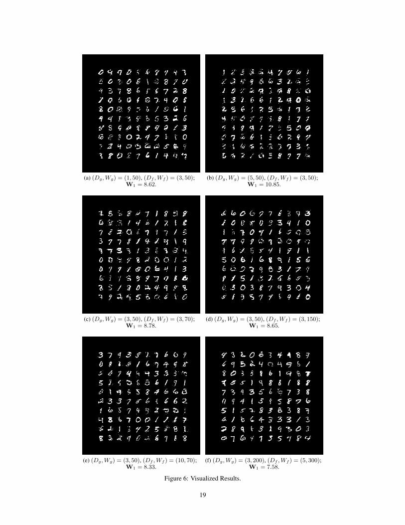
(a) (Dg,Wg) = (1, 50), (Df ,Wf ) = (3, 50);W1 = 8.62.

(b) (Dg,Wg) = (5, 50), (Df ,Wf ) = (3, 50);W1 = 10.85.

(c) (Dg,Wg) = (3, 50), (Df ,Wf ) = (3, 70);W1 = 8.78.

(d) (Dg,Wg) = (3, 50), (Df ,Wf ) = (3, 150);W1 = 8.65.

(e) (Dg,Wg) = (3, 50), (Df ,Wf ) = (10, 70);W1 = 8.33.

(f) (Dg,Wg) = (3, 200), (Df ,Wf ) = (5, 300);W1 = 7.58.

Figure 6: Visualized Results.

19

approximation capabilities of wasserstein generative

Documents