Multiparty Computation from Somewhat HomomorphicEncryption

Ivan Damgard1, Valerio Pastro1, Nigel Smart2, and Sarah Zakarias1

1 Department of Computer Science, Aarhus University2 Department of Computer Science, Bristol University

Abstract. We propose a general multiparty computation protocol secure against an active adversarycorrupting up to n−1 of the n players. The protocol may be used to compute securely arithmetic circuitsover any finite field Fpk . Our protocol consists of a preprocessing phase that is both independent of thefunction to be computed and of the inputs, and a much more efficient online phase where the actualcomputation takes place. The online phase is unconditionally secure and has total computational (andcommunication) complexity linear in n, the number of players, where earlier work was quadratic in n.Moreover, the work done by each player is only a small constant factor larger than what one wouldneed to compute the circuit in the clear. We show this is optimal for computation in large fields. Inpractice, for 3 players, a secure 64-bit multiplication can be done in 0.05 ms. Our preprocessing is basedon a somewhat homomorphic cryptosystem. We extend a scheme by Brakerski et al., so that we canperform distributed decryption and handle many values in parallel in one ciphertext. The computationalcomplexity of our preprocessing phase is dominated by the public-key operations, we need O(n2/s)operations per secure multiplication where s is a parameter that increases with the security parameterof the cryptosystem. Earlier work in this model needed Ω(n2) operations. In practice, the preprocessingprepares a secure 64-bit multiplication for 3 players in about 13 ms.

1 Introduction

A central problem in theoretical cryptography is that of secure multiparty computation (MPC).In this problem n parties, holding private inputs x1, . . . , xn, wish to compute a given functionf(x1, . . . , xn). A protocol for doing this securely should be such that honest players get the correctresult and this result is the only new information released, even if some subset of the players iscontrolled by an adversary.

In the case of dishonest majority, where more than half the players are corrupt, unconditionallysecure protocols cannot exist. Under computational assumptions, it was shown in [8] how to con-struct UC-secure MPC protocols that handle the case where all but one of the parties are activelycorrupted. The public-key machinery one needs for this is typically expensive so efficient solutionsare hard to design for dishonest majority. Recently, however, a new approach has been proposedmaking such protocols more practical. This approach works as follows: one first designs a generalMPC protocol in the preprocessing model, where access to a “trusted dealer” is assumed. The dealerdoes not need to know the function to be computed, nor the inputs, he just supplies raw materialfor the computation before it starts. This allows the “online” protocol to use only cheap informationtheoretic primitives and hence be efficient. Finally, one implements the trusted dealer by a secureprotocol using public-key techniques, this protocol can then be run in a preprocessing phase. Thecurrent state of the art in this respect are the protocols in Bendlin et al., Damgard/Orlandi andNielsen et al. [5, 13, 25]. The “MPC-in-the-head” technique of Ishai et al. [18, 17] has similar overallasymptotic complexity, but larger constants and a less efficient online phase.

Recently, another approach has become possible with the advent of Fully Homomorphic En-cryption (FHE) by Gentry [15]. In this approach all parties first encrypt their input under the

FHE scheme; then they evaluate the desired function on the ciphertexts using the homomorphicproperties, and finally they perform a distributed decryption on the final ciphertexts to get theresults. The advantage of the FHE-based approach is that interaction is only needed to supplyinputs and get output. However, the low bandwidth consumption comes at a price; current FHEschemes are very slow and can only evaluate small circuits, i.e., they actually only provide whatis known as somewhat homomorphic encryption (SHE). This can be circumvented in two ways;either by assuming circular security and implementing an expensive bootstrapping operation, orby extending the parameter sizes to enable a “levelled FHE” scheme which can evaluate circuits oflarge degree (exponential in the number of levels) [6]. The main cost, much like other approaches, isin terms of the number of multiplications in the arithmetic circuit. So whilst theoretically appealingthe approach via FHE is not competitive in practice with the traditional MPC approach.

1.1 Contributions of this paper.

Optimal Online Phase. We propose an MPC protocol in the preprocessing model that computessecurely an arithmetic circuit C over any finite field Fpk . The protocol is statistically UC-secureagainst active and adaptive corruption of up to n− 1 of the n players, and we assume synchronouscommunication and secure point-to-point channels. Measured in elementary operations in Fpk thetotal amount of work done is O(n · |C|+n3) where |C| is the size of C. All earlier work in this modelhad complexity Ω(n2 · |C|). A similar improvement applies to the communication complexity andthe amount of data one needs to store from the preprocessing. Hence, the work done by each playerin the online phase is essentially independent of n. Moreover, it is only a small constant factorlarger than what one would need to compute the circuit in the clear. This is the first protocol inthe preprocessing model with these properties3.

Finally, we show a lower bound implying that w.r.t the amount of data required from thepreprocessing, our protocol is optimal up to a constant factor. We also obtain a similar lowerbound on the number of bit operations required, and hence the computational work done in ourprotocol is optimal up to poly-logarithmic factors.

All results mentioned here hold for the case of large fields, i.e., where the desired error probabilityis (1/pk)c, for a small constant c. Note that many applications of MPC need integer arithmetic,modular reductions, conversion to binary, etc., which we can emulate by computing in Fp with plarge enough to avoid overflow. This naturally leads to computing with large fields. As mentioned,our protocol works for all fields, but like earlier work in this model it is less efficient for small fieldsby a factor of essentially d sec

log pke for error probability 2−Θ(sec), see Appendix A.4 for details.

Obtaining our result requires new ideas compared to [5], which was previously state of the artand was based on additive secret sharing where each share in a secret is authenticated using aninformation theoretic Message Authentication Code (MAC). Since each player needs to have hisown key, each of the n shares need to be authenticated with n MACs, so this approach is inherentlyquadratic in n. Our idea is to authenticate the secret value itself instead of the shares, using asingle global key. This seems to lead to a “chicken and egg” problem since one cannot check aMAC without knowing the key, but if the key is known, MACs can be forged. Our solution to this

3 With dishonest majority, successful termination cannot be guaranteed, so our protocols simply abort if cheating isdetected. We do not, however, identify who cheated, indeed the standard definition of secure function evaluationdoes not require this. Identification of cheaters is possible but we do not know how to do this while maintainingcomplexity linear in n.

2

involves secret sharing the key as well, carefully timing when values are revealed, and various tricksto reduce the amortized cost of checking a set of MACs.

Efficient use of FHE for MPC. As a conceptual contribution we propose what we believe is “theright” way to use FHE/SHE for computationally efficient MPC, namely to use it for implementinga preprocessing phase. The observation is that since such preprocessing is typically based on theclassic circuit randomization technique of Beaver [3], it can be done by evaluating in parallel manysmall circuits of small multiplicative depth (in fact depth 1 in our case). Thus SHE suffices, we donot need bootstrapping, and we can use the SHE SIMD approach of [27] to handle many values inparallel in a single ciphertext.

To capitalize on this idea, we apply the SIMD approach to the cryptosystem from [7] (see also[16] where this technique is also used). To get the best performance, we need to do a non-trivialanalysis of the parameter values we can use, and we prove some results on norms of embeddingsof a cyclotomic field for this purpose. We also design a distributed decryption procedure for ourcryptosystem. This protocol is only robust against passive attacks. Nevertheless, this is sufficient forthe overall protocol to be actively secure. Intuitively, this is because the only damage the adversarycan do is to add a known error term to the decryption result obtained. The effect of this for theonline protocol is that certain shares of secret values may be incorrect, but this will caught bythe check involving the MACs. Finally we adapt a zero-knowledge proof of plaintext knowledgefrom [5] for our purpose and in particular we improve the analysis of the soundness guarantees itoffers. This influences the choice of parameters for the cryptosystem and therefore improves overallperformance.

An Efficient Preprocessing Protocol. As a result of the above, we obtain a constant-round prepro-cessing protocol that is UC-secure against active and static corruption of n − 1 players assumingthe underlying cryptosystem is semantically secure, which follows from the polynomial (PLWE)assumption. UC-security for dishonest majority cannot be obtained without a set-up assumption.In this paper we assume that a key pair for our cryptosystem has been generated and the secretkey has been shared among the players.

Whereas previous work in the preprocessing/online model [5, 13] use Ω(n2) public-key opera-tions per secure multiplication, we only need O(n2/s) operations, where s is a number that growswith the security parameter of the SHE scheme (we have s ≈ 12000 in our concrete instantiationfor computing in Fp where p ≈ 264). We stress that our adapted scheme is exactly as efficient as thebasic version of [7] that does not allow this optimization, so the improvement is indeed “genuine”.

In comparison to the approach mentioned above where one uses FHE throughout the protocol,our combined preprocessing and online phase achieves a result that is incomparable from a theo-retical point of view, but much more practical: we need more communication and rounds, but thecomputational overhead is much smaller – we need O(n2/s · |C|) public key operations comparedto O(n · |C|) for the FHE approach, where for realistic values of n and s, we have n2/s n.Furthermore, we only need a low depth SHE which is much more efficient in the first place. Andfinally, we can push all the work using SHE into a, function independent, preprocessing phase.

Performance in practice. Both the preprocessing and online phase have been implemented andtested for 3 players on up-to-date machines connected on a LAN. The preprocessing takes about13 ms amortized time to prepare one multiplication in Fp for a 64-bit p, with security level corre-sponding roughly to 1024 bit RSA and an error probability of 2−40 for the zero-knowledge proofs

3

(the error probability can be lowered to 2−80 by repeating the ZK proofs which will at most doublethe time). This is 2-3 orders of magnitude faster than preliminary estimates for the most efficientinstantiation of [5]. The online phase executes a secure 64-bit multiplication in 0.05 ms amortizedtime. These rough orders of magnitude, and the ability to deal with a non-trivial number of players,are born out by a recent implementation of the protocols described in this paper [11].

Concurrent Related Work. In recent independent work [24, 2, 16], Meyers at al., Asharov et al.and Gentry et al. also use an FHE scheme for multiparty computation. They follow the pure FHEapproach mentioned above, using a threshold decryption protocol tailored to the specific FHEscheme. They focus primarily on round complexity, while we want to minimize the computationaloverhead. We note that in [16], Gentry et al. obtain small overhead by showing a way to use theFHE SIMD approach for computing any circuit homomorphically. However, this requires full FHEwith bootstrapping (to work on arbitrary circuits) and does not (currently) lead to a practicalprotocol.

In [25], Nielsen et al. consider secure computing for Boolean Circuits. Their online phase issimilar to that of [5], while the preprocessing is a clever and very efficient construction based onOblivious Transfer. This result is complementary to ours in the sense that we target computationsover large fields which is good for some applications whereas for other cases, Boolean Circuits are themost compact way to express the desired computation. Of course, one could use the preprocessingfrom [25] to set up data for our online phase, but current benchmarks indicate that our approachis faster for large fields, say of size 64 bits or more.

We end the introduction by covering some basic notation which will be used throughout thispaper. For a vector x = (x1, . . . , xn) ∈ Rn we denote by ‖x‖∞ := max1≤i≤n |xi|, ‖x‖1 :=

∑1≤i≤n |xi|

and ‖x‖2 :=√∑

|xi|2. We let ε(κ) denote an unspecified negligible function of κ. If S is a set welet x← S denote assignment to the variable x with respect to a uniform distribution on S; we usex ← s for a value s as shorthand for x ← s. If A is an algorithm x ← A means assign to x theoutput of A, where the probability distribution is over the random coins of A. Finally x := y means“x is defined to be y”.

2 Online Protocol

Our aim is to construct a protocol for arithmetic multiparty computation over Fpk for some primep. More precisely, we wish to implement the ideal functionality FAMPC, presented in Figure 15 inAppendix Ethe full version. Our MPC protocol is structured in a preprocessing (or offline) phaseand an online phase. We start out in this section by presenting the online phase which assumesaccess to an ideal functionality FPREP (Figure 16 of Appendix E). In Section 5 we show how toimplement this functionality in an independent preprocessing phase.

In our specification of the online protocol, we assume for simplicity that a broadcast channelis available at unit cost, that each party has only one input, and only one public output valueis to be computed. In Appendix A.3 we explain how to implement the broadcasts we need frompoint-to-point channels and lift the restriction on the number of inputs and outputs without thisaffecting the overall complexity.

Before presenting the concrete online protocol we give the intuition and motivation behindthe construction. We will use unconditionally secure MACs to protect secret values from beingmanipulated by an active adversary. However, rather than authenticating shares of secret values as

4

in [5], we authenticate the shared value itself. More concretely, we will use a global key α chosenrandomly in Fpk , and for each secret value a, we will share a additively among the players, and wealso secret-share a MAC αa. This way to represent secret values is linear, just like the representationin [5], and we can therefore do secure multiplication based on multiplication triples a la Beaver [3]that we produce in the preprocessing.

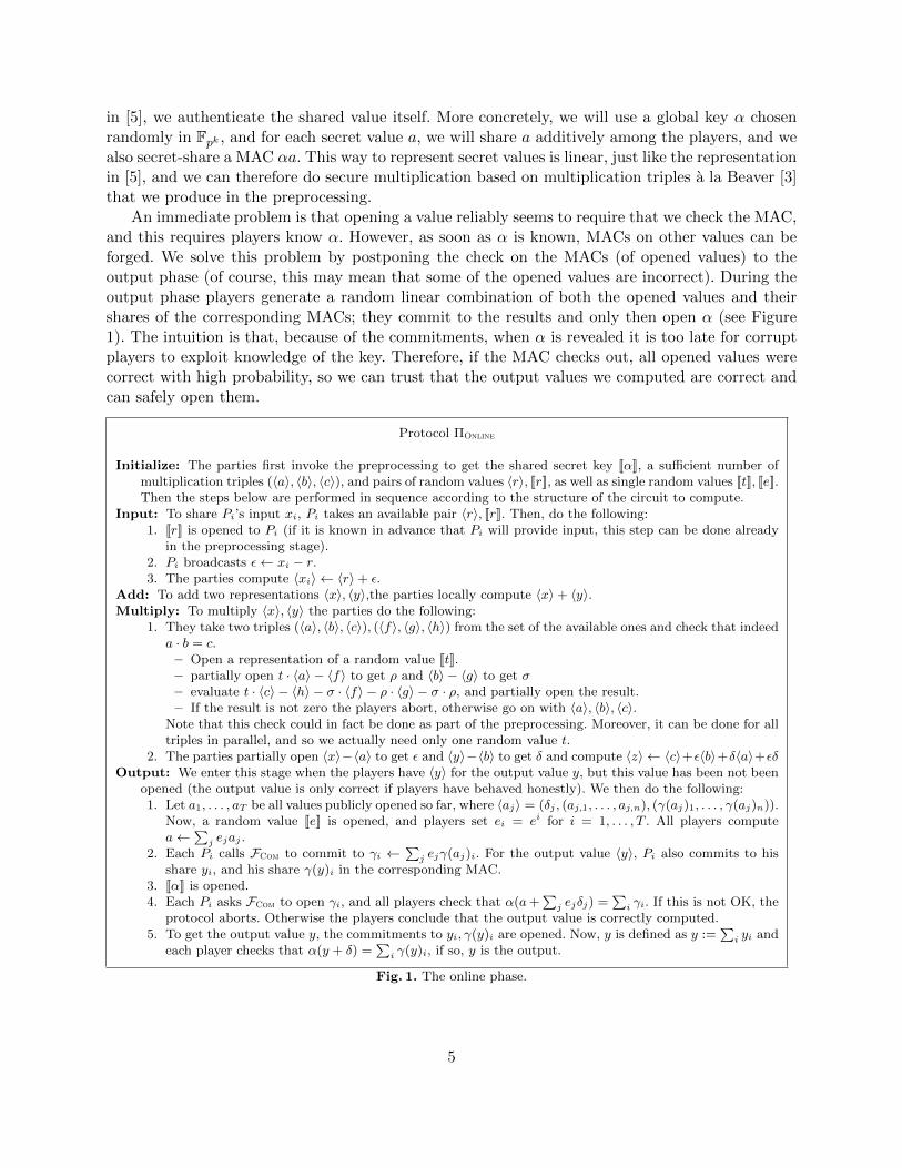
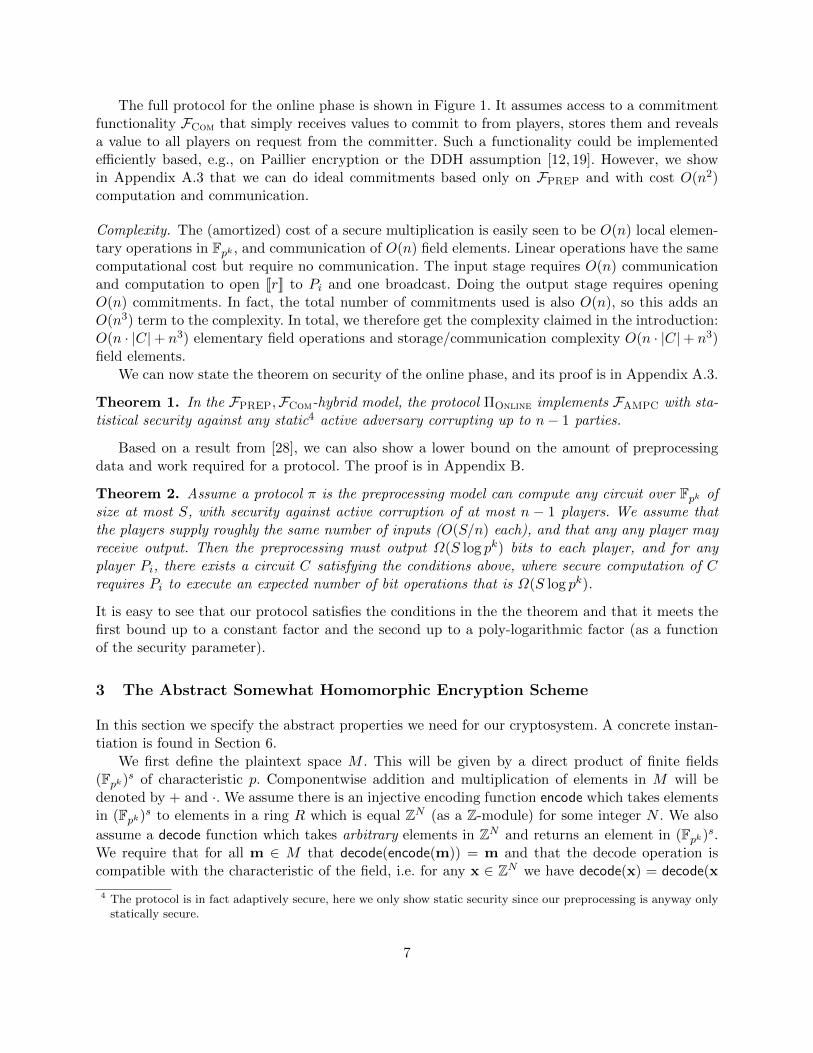
An immediate problem is that opening a value reliably seems to require that we check the MAC,and this requires players know α. However, as soon as α is known, MACs on other values can beforged. We solve this problem by postponing the check on the MACs (of opened values) to theoutput phase (of course, this may mean that some of the opened values are incorrect). During theoutput phase players generate a random linear combination of both the opened values and theirshares of the corresponding MACs; they commit to the results and only then open α (see Figure1). The intuition is that, because of the commitments, when α is revealed it is too late for corruptplayers to exploit knowledge of the key. Therefore, if the MAC checks out, all opened values werecorrect with high probability, so we can trust that the output values we computed are correct andcan safely open them.

Protocol ΠOnline

Initialize: The parties first invoke the preprocessing to get the shared secret key [[α]], a sufficient number ofmultiplication triples (〈a〉, 〈b〉, 〈c〉), and pairs of random values 〈r〉, [[r]], as well as single random values [[t]], [[e]].Then the steps below are performed in sequence according to the structure of the circuit to compute.

Input: To share Pi’s input xi, Pi takes an available pair 〈r〉, [[r]]. Then, do the following:1. [[r]] is opened to Pi (if it is known in advance that Pi will provide input, this step can be done already

in the preprocessing stage).2. Pi broadcasts ε← xi − r.3. The parties compute 〈xi〉 ← 〈r〉+ ε.

Add: To add two representations 〈x〉, 〈y〉,the parties locally compute 〈x〉+ 〈y〉.Multiply: To multiply 〈x〉, 〈y〉 the parties do the following:

1. They take two triples (〈a〉, 〈b〉, 〈c〉), (〈f〉, 〈g〉, 〈h〉) from the set of the available ones and check that indeeda · b = c.– Open a representation of a random value [[t]].– partially open t · 〈a〉 − 〈f〉 to get ρ and 〈b〉 − 〈g〉 to get σ– evaluate t · 〈c〉 − 〈h〉 − σ · 〈f〉 − ρ · 〈g〉 − σ · ρ, and partially open the result.– If the result is not zero the players abort, otherwise go on with 〈a〉, 〈b〉, 〈c〉.

Note that this check could in fact be done as part of the preprocessing. Moreover, it can be done for alltriples in parallel, and so we actually need only one random value t.

2. The parties partially open 〈x〉−〈a〉 to get ε and 〈y〉−〈b〉 to get δ and compute 〈z〉 ← 〈c〉+ε〈b〉+δ〈a〉+εδOutput: We enter this stage when the players have 〈y〉 for the output value y, but this value has been not been

opened (the output value is only correct if players have behaved honestly). We then do the following:1. Let a1, . . . , aT be all values publicly opened so far, where 〈aj〉 = (δj , (aj,1, . . . , aj,n), (γ(aj)1, . . . , γ(aj)n)).

Now, a random value [[e]] is opened, and players set ei = ei for i = 1, . . . , T . All players computea←

∑j ejaj .

2. Each Pi calls FCom to commit to γi ←∑j ejγ(aj)i. For the output value 〈y〉, Pi also commits to his

share yi, and his share γ(y)i in the corresponding MAC.3. [[α]] is opened.4. Each Pi asks FCom to open γi, and all players check that α(a+

∑j ejδj) =

∑i γi. If this is not OK, the

protocol aborts. Otherwise the players conclude that the output value is correctly computed.5. To get the output value y, the commitments to yi, γ(y)i are opened. Now, y is defined as y :=

∑i yi and

each player checks that α(y + δ) =∑i γ(y)i, if so, y is the output.

Fig. 1. The online phase.

5

Representation of values and MACs. In the online phase each shared value a ∈ Fpk is representedas follows

〈a〉 := (δ, (a1, . . . , an), (γ(a)1, . . . , γ(a)n))

where a = a1 + · · ·+an and γ(a)1 + · · ·+γ(a)n = α(a+ δ). Player Pi holds ai, γ(a)i and δ is public.The interpretation is that γ(a)← γ(a)1 + · · ·+γ(a)n is the MAC authenticating a under the globalkey α.

Computations. Using the natural component-wise addition of representations, and suppressingthe underlying choices of ai, γ(a)i for readability, we clearly have for secret values a, b and publicconstant e that

〈a〉+ 〈b〉 = 〈a+ b〉 e · 〈a〉 = 〈ea〉, and e+ 〈a〉 = 〈e+ a〉,

where e+〈a〉 := (δ−e, (a1+e, a2, . . . , an), (γ(a)1, . . . , γ(a)n)). This possibility to easily add a publicvalue is the reason for the “public modifier” δ in the definition of 〈·〉. It is now clear that we cando secure linear computations directly on values represented this way.

What remains is multiplications: here we use the preprocessing. We would like the preprocessingto output random triples 〈a〉, 〈b〉, 〈c〉, where c = ab. However, our preprocessing produces tripleswhich satisfy c = ab+∆, where ∆ is an error that can be introduced by the adversary. We thereforeneed to check the triple before we use it. The check can be done by “sacrificing” another triple〈f〉, 〈g〉, 〈h〉, where the same multiplicative equality should hold (see the protocol for details). Givensuch a valid triple, we can do multiplications in the following standard way: To compute 〈xy〉 wefirst open 〈x〉 − 〈a〉 to get ε, and 〈y〉 − 〈b〉 to get δ. Then xy = (a + ε)(b + δ) = c + εb + δa + εδ.Thus, the new representation can be computed as

〈x〉 · 〈y〉 = 〈c〉+ ε〈b〉+ δ〈a〉+ εδ.

An important note is that during our protocol we are actually not guaranteed that we areworking with the correct results, since we do not immediately check the MACs of the openedvalues. During the first part of the protocol, parties will only do what we define as a partialopening, meaning that for a value 〈a〉, each party Pi sends ai to P1, who computes a = a1 + · · ·+anand broadcasts a to all players. We assume here for simplicity that we always go via P1, whereasin practice, one would balance the workload over the players.

As sketched earlier we postpone the checking to the end of the protocol in the output phase.To check the MACs we need the global key α. We get α from the preprocessing but in a slightlydifferent representation:

[[α]] := ((α1, . . . , αn), (βi, γ(α)i1, . . . , γ(α)in)i=1,...,n)),

where α =∑

i αi and∑

j γ(α)ji = αβi. Player Pi holds αi, βi, γ(α)i1, . . . , γ(α)in. The idea is that

γ(α)i ←∑

j γ(α)ji is the MAC authenticating α under Pi’s private key βi. To open [[α]] each Pj

sends to each Pi his share αj of α and his share γ(α)ji of the MAC on α made with Pi’s private

key and then Pi checks that∑

j γ(α)ji = αβi. (To open the value to only one party Pi, the otherparties will simply send their shares only to Pi, who will do the checking. Only shares of α and αβiare needed.)

Finally, the preprocessing will also output n pairs of a random value r in both of the presentedrepresentations 〈r〉, [[r]]. These pairs are used in the Input phase of the protocol.

6

The full protocol for the online phase is shown in Figure 1. It assumes access to a commitmentfunctionality FCom that simply receives values to commit to from players, stores them and revealsa value to all players on request from the committer. Such a functionality could be implementedefficiently based, e.g., on Paillier encryption or the DDH assumption [12, 19]. However, we showin Appendix A.3 that we can do ideal commitments based only on FPREP and with cost O(n2)computation and communication.

Complexity. The (amortized) cost of a secure multiplication is easily seen to be O(n) local elemen-tary operations in Fpk , and communication of O(n) field elements. Linear operations have the samecomputational cost but require no communication. The input stage requires O(n) communicationand computation to open [[r]] to Pi and one broadcast. Doing the output stage requires openingO(n) commitments. In fact, the total number of commitments used is also O(n), so this adds anO(n3) term to the complexity. In total, we therefore get the complexity claimed in the introduction:O(n · |C|+ n3) elementary field operations and storage/communication complexity O(n · |C|+ n3)field elements.

We can now state the theorem on security of the online phase, and its proof is in Appendix A.3.

Theorem 1. In the FPREP,FCom-hybrid model, the protocol ΠOnline implements FAMPC with sta-tistical security against any static4 active adversary corrupting up to n− 1 parties.

Based on a result from [28], we can also show a lower bound on the amount of preprocessingdata and work required for a protocol. The proof is in Appendix B.

Theorem 2. Assume a protocol π is the preprocessing model can compute any circuit over Fpk ofsize at most S, with security against active corruption of at most n − 1 players. We assume thatthe players supply roughly the same number of inputs (O(S/n) each), and that any any player mayreceive output. Then the preprocessing must output Ω(S log pk) bits to each player, and for anyplayer Pi, there exists a circuit C satisfying the conditions above, where secure computation of Crequires Pi to execute an expected number of bit operations that is Ω(S log pk).

It is easy to see that our protocol satisfies the conditions in the the theorem and that it meets thefirst bound up to a constant factor and the second up to a poly-logarithmic factor (as a functionof the security parameter).

3 The Abstract Somewhat Homomorphic Encryption Scheme

In this section we specify the abstract properties we need for our cryptosystem. A concrete instan-tiation is found in Section 6.

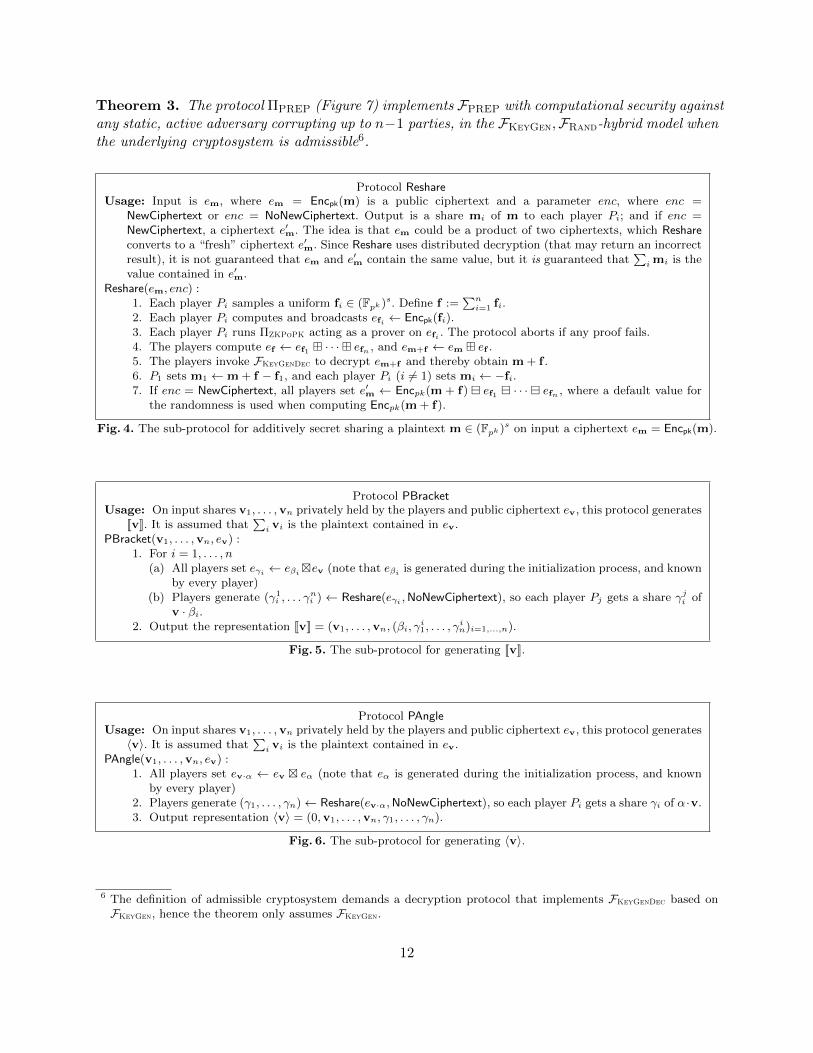
We first define the plaintext space M . This will be given by a direct product of finite fields(Fpk)s of characteristic p. Componentwise addition and multiplication of elements in M will bedenoted by + and ·. We assume there is an injective encoding function encode which takes elementsin (Fpk)s to elements in a ring R which is equal ZN (as a Z-module) for some integer N . We also

assume a decode function which takes arbitrary elements in ZN and returns an element in (Fpk)s.We require that for all m ∈ M that decode(encode(m)) = m and that the decode operation iscompatible with the characteristic of the field, i.e. for any x ∈ ZN we have decode(x) = decode(x

4 The protocol is in fact adaptively secure, here we only show static security since our preprocessing is anyway onlystatically secure.

7

(mod p)). And finally that the encoding function produces “short” vectors. More precisely, that forall m ∈ (Fpk)s ‖encode(m)‖∞ ≤ τ where τ = p/2.

The two operations in R will be denoted by + and ·. The addition operation in R is assumedto be componentwise addition, whereas we make no assumption on multiplication. All we requireis that the following properties hold, for all elements m1,m2 ∈M ;

decode(encode(m1) + encode(m2)) = m1 + m2,

decode(encode(m1) · encode(m2)) = m1 ·m2.

From now on, when we discuss the plaintext space M we assume it comes implicitly with the encodeand decode functions for some integer N . If an element in M has the same component in each ofthe s-slots, then we call it a “diagonal” element. We let Diag(x) for x ∈ Fpk denote the element(x, x, . . . , x) ∈ (Fpk)s.

Our cryptosystem consists of a tuple (ParamGen,KeyGen,KeyGen∗,Enc,Dec) of algorithms de-fined below, and parametrized by a security parameter κ.ParamGen(1κ,M): This parameter generation algorithm outputs an integer N (as above), definitions

of the encode and decode functions, and a description of a randomized algorithm Ddρ, which outputs

vectors in Zd. We assume that Ddρ outputs r with ‖r‖∞ ≤ ρ, except with negligible probability.

The algorithm Ddρ is used by the encryption algorithm to select the random coins needed duringencryption. The algorithm ParamGen also outputs an additive abelian group G. The group G alsopossesses a (not necessarily closed) multiplicative operator, which is commutative and distributesover the additive group of G. The group G is the group in which the ciphertexts will be assumed tolie. We write and for the operations on G, and extend these in the natural way to vectors andmatrices of elements of G. Finally ParamGen outputs a set C of allowable arithmetic SIMD circuitsover (Fpk)s, these are the set of functions which our scheme will be able to evaluate ciphertextsover. We can think of C as a subset of Fpk [X1, X2, . . . , Xn], where we evaluate a function f ∈Fpk [X1, X2, . . . , Xn] a total of s times in parallel on inputs from (Fpk)n. We assume that all other

algorithms take as implicit input the output P ← (1κ, N, encode, decode,Ddρ, G,C) of ParamGen.KeyGen(): This algorithm outputs a public key pk and a secret key sk.

Encpk(x, r): On input of x ∈ ZN , r ∈ Zd, this deterministic algorithm outputs a ciphertext c ∈ G.When applying this algorithm one would obtain x from the application of the encode function,and r by calling Ddρ. This is what we mean when we write Encpk(m), where m ∈ M . However,it is convenient for us to define Enc on the intermediate state, x = encode(m). To ease notationwe write Encpk(x) if the value of the randomness r is not important for our discussion. To makeour zero-knowledge proofs below work, we will require that addition of V “clean” ciphertexts (for“small” values of V ), of plaintext xi in ZN , using randomness ri, results in a ciphertext whichcould be obtained by adding the plaintexts and randomness, as integer vectors, and then applyingEncpk(x, r), i.e.

Encpk(x1 + · · ·+ xV , r1 + · · ·+ rV ) = Encpk(x1, r1) · · · Encpk(xV , rV ).

Decsk(c): On input the secret key and a ciphertext c it returns either an element m ∈ M , or thesymbol ⊥.

We are now able to define various properties of the above abstract scheme that we will require. Butfirst a bit of notation: For a function f ∈ C we let n(f) denote the number of variables in f , and we

8

let f denote the function on G induced by f . That is, given f , we replace every + operation with a, every · operation is replaced with a and every constant c is replaced by Encpk(encode(c),0).Also, given a set of n(f) vectors x1, . . . ,xn(f), we define f(x1, . . . ,xn(f)) in the natural way byapplying f in parallel on each coordinate.

Correctness: Intuitively correctness means that if one decrypts the result of a function f ∈ Capplied to n(f) encrypted vectors of variables, then this should return the same value as applyingthe function to the n(f) plaintexts. However, to apply the scheme in our protocol, we need tobe a bit more liberal, namely the decryption result should be correct, even if the ciphertexts westart from were not necessarily generated by the normal encryption algorithm. They only need to“contain” encodings and randomness that are not too large, such that the encodings decode to legalvalues. Formally, the scheme is said to be (Bplain, Brand, C)-correct if

Pr [P ← ParamGen(1κ,M), (pk, sk)← KeyGen(), for any f ∈ C,any xi, ri, with ‖xi‖∞ ≤ Bplain, ‖ri‖∞ ≤ Brand, decode(xi) ∈ (Fpk)s,

i = 1, . . . , n(f), and ci ← Encpk(xi, ri), c← f(c1, . . . , cn(f)) :

Decsk(c) 6= f(decode(x1), . . . , decode(xn(f))) ] < ε(κ).

We will say that a ciphertext is (Bplain, Brand, C)-admissible if it can be obtained as the ciphertextc in the above experiment, i.e., by applying a function from C to ciphertexts generated from (legal)encodings and randomness that are bounded by Bplain and Brand.

KeyGen∗(): This is a randomized algorithm that outputs a meaningless public key pk. We requirethat an encryption of any message Enc

pk(x) is statistically indistinguishable from an encryption of 0.

Furthermore, if we set (pk, sk)← KeyGen() and pk← KeyGen∗(), then pk and pk are computationallyindistinguishable. This implies the scheme is IND-CPA secure in the usual sense.

Distributed Decryption: We assume, as a set up assumption, that a common public key has beenset up where the secret key has been secret-shared among the players in such a way that they cancollaborate to decrypt a ciphertext. We assume throughout that only (Bplain, Brand, C)-admissibleciphertexts are to be decrypted, this constraint is guaranteed by our main protocol.

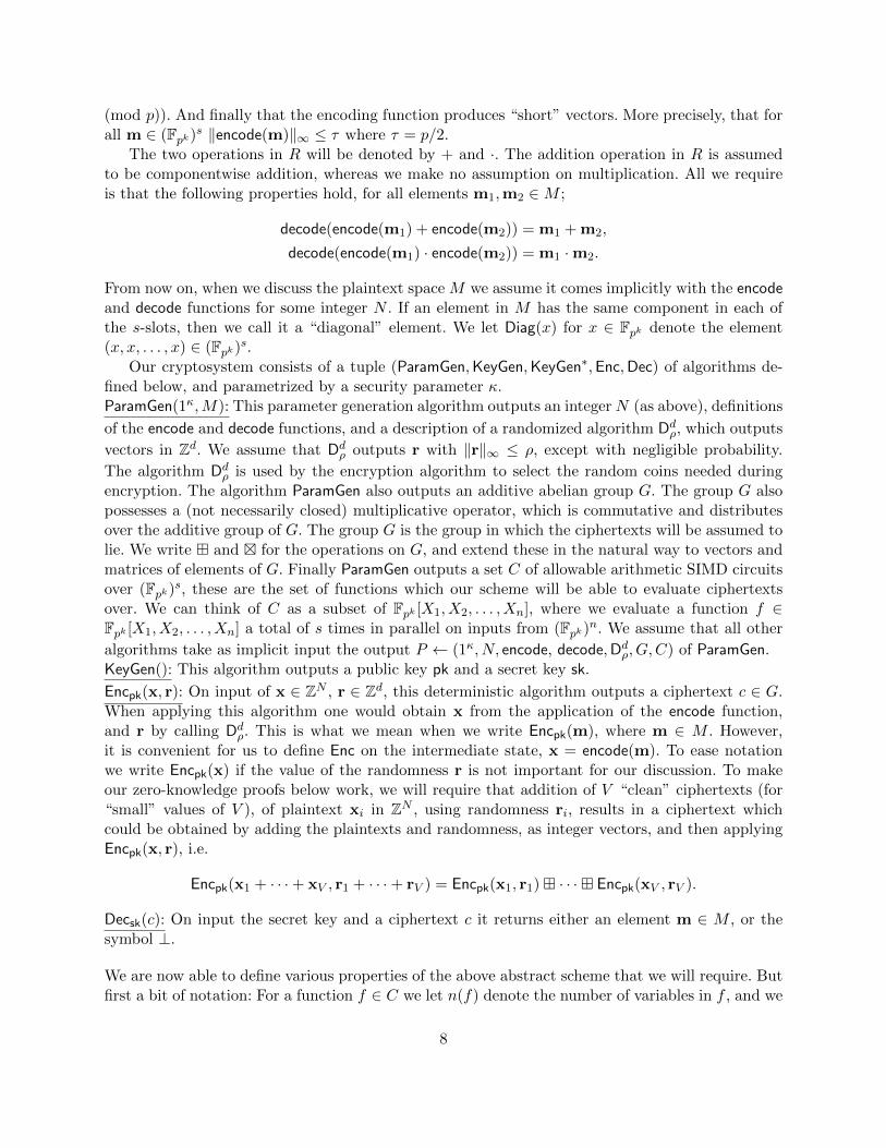
We note that some set-up assumption is always required to show UC security which is our goalhere. Concretely, we assume that a functionality FKeyGen is available, as specified in Figure 2. Itbasically generates a key pair and secret-shares the secret key among the players using a secret-sharing scheme that is assumed to be given as part of the specification of the cryptosystem. Sincewe want to allow corruption of all but one player, the maximal unqualified sets must be all sets ofn− 1 players.

Functionality FKeyGen

1. When receiving “start” from all honest players, run P ← ParamGen(1κ,M), and then, using the parametersgenerated, run (pk, sk)← KeyGen() (recall P , and hence 1κ, is an implicit input to all functions we specify).Send pk to the adversary.

2. We assume a secret sharing scheme is given with which sk can be secret-shared. Receive from the adversarya set of shares sj for each corrupted player Pj .

3. Construct a complete set of shares (s1, . . . , sn) consistent with the adversary’s choices and sk. Note that thisis always possible since the corrupted players form an unqualified set. Send pk to all players and si to eachhonest Pi.

Fig. 2. The Ideal Functionality for Distributed Key Generation

9

We note that it is possible to make a weaker set-up assumption, such as a common referencestring (CRS), and using a general UC secure multiparty computation protocol for the CRS modelto implement FKeyGen. While this may not be very efficient, one only needs to run this protocolonce in the life-time of the system.

We also want our cryptosystem to implement the functionality FKeyGenDec in Figure 3, whichessentially specifies that players can cooperate to decrypt a (Bplain, Brand, C)-admissible ciphertext,but the protocol is only secure against a passive attack: the adversary gets the correct decryptionresult, but can decide which result the honest players should learn.

Functionality FKeyGenDec

1. When receiving “start” from all honest players, run ParamGen(1κ,M), and then, using the parametersgenerated, run (pk, sk)← KeyGen(). Send pk to the adversary and to all players, and store sk.

2. Hereafter on receiving “decrypt c” for (Bplain, Brand, C)-admissible c from all honest players, send c andm ← Decsk(c) to the adversary. On receiving m′ from the adversary, send “Result m′” to all players, Bothm and m′ may be a special symbol ⊥ indicating that decryption failed.

3. On receiving “decrypt c to Pj” for admissible c, if Pj is corrupt, send c,m ← Decsk(c) to the adversary. IfPj is honest, send c to the adversary. On receiving δ from the adversary, if δ 6∈ M , send ⊥ to Pj , if δ ∈ M ,send Decsk(c) + δ to Pj .

Fig. 3. The Ideal Functionality for Distributed Key Generation and Decryption

We are now finally ready to define the basic set of properties that the underlying cryptosystemshould satisfy, in order to be used in our protocol. Here we use an “information theoretic” securityparameter sec that controls the errors in our ZK proofs below.

Definition 1. (Admissible Cryptosystem.) Let C contain formulas of form (x1 + · · · + xn) ·(y1 + · · · + yn) + z1 + · · · + zn, as well as all “smaller” formulas , i.e., with a smaller number ofadditions and possibly no multiplication. A cryptosystem is admissible if it is defined by algorithms(ParamGen,KeyGen,KeyGen∗,Enc, Dec) with properties as defined above, is (Bplain, Brand, C)-correct,where

Bplain = N · τ · sec2 · 2(1/2+ν)sec, Brand = d · ρ · sec2 · 2(1/2+ν)sec;

and where ν > 0 can be an arbitrary constant. Finally there exist a secret sharing scheme asrequired in FKeyGen and a protocol ΠKeyGenDec with the property that when composed with FKeyGen

it securely implements the functionality FKeyGenDec.

The set C is defined to contain all computations on ciphertext that we need in our main protocol.Throughout the paper we will assume that Bplain, Brand are defined as here in terms of τ, ρ and sec.This is because these are the bounds we can force corrupt players to respect via our zero-knowledgeprotocol, as we shall see.

4 Zero-Knowledge Proof of Plaintext Knowledge

This section presents a zero-knowledge protocol that takes as input sec ciphertexts c1, . . . , csecgenerated by one of the players in our protocol, who will act as the prover. If the prover is honestthen ci = Encpk(xi, ri), where xi has been obtained from the encode function, i.e. ‖xi‖∞ ≤ τ , and ri

10

has been generated from Ddρ (so we may assume that ‖ri‖∞ ≤ ρ). Our protocol is a zero-knowledgeproof of plaintext knowledge (ZKPoPK) for the following relation:

RPoPK = (x,w)| x = (pk, c), w = ((x1, r1), . . . , (xsec, rsec)) :

c = (c1, . . . , csec), ci ← Encpk(xi, ri),

‖xi‖∞ ≤ Bplain, decode(xi) ∈ (Fpk)s, ‖ri‖∞ ≤ Brand .

The zero-knowledge and completeness properties hold only if the ciphertexts ci satisfy ‖xi‖∞ ≤ τand ‖ri‖∞ ≤ ρ.

In our preprocessing protocol, players will be required to give such a ZKPoPK for all ciphertextsthey provide. By admissibility of the cryptosystem, this will imply that every ciphertext occurringin the protocol will be (Bplain, Brand, C)-admissible and can therefore be decrypted correctly. TheZKPoPK can also be called with a flag diag which will modify the proof so that it additionallyproves that decode(xi) is a diagonal element.

The protocol is not meant to implement an ideal functionality, but we can still use it and proveUC security for the main protocol, since we will always generate the challenge e by calling the FRand

ideal functionality (see Appendix E). Hence the honest-verifier ZK property implies straight-linesimulation5. As for knowledge extraction, the UC simulator we construct in our security proof willknow the secret key for the cryptosystem and can therefore extract a dishonest prover’s witnesssimply by decrypting. In the reduction to show that the simulator works, we do not know the secretkey, but here we are allowed to do extraction by rewinding.

The protocol and its proof of security are given in Appendix A.1, Figure 9 and its computationalcomplexity per ciphertext is essentially the cost of a constant number of encryptions. In AppendixA.1, we also give a variant of the ZK proof that allows even smaller values for Bplain, Brand, namelyBplain = N · τ · sec2 · 2sec/2+8, Brand = d · ρ · sec2 · 2sec/2+8, and hence improves performance further.This variant is most efficient when executed using the Fiat-Shamir heuristic (although it can alsowork without random oracles), and we believe this variant is the best for a practical implementation.

5 The Preprocessing Phase

In this section we construct the protocol ΠPREP which securely implements the functionality FPREP

(specified in Figure 16) in the presence of functionalities FKeyGenDec (Figure 3) and FRand (Figure14). The preprocessing uses the above abstract cryptosystem with M = (Fpk)s, but the onlinephase is designed for messages in Fpk . Therefore, we extend the notation 〈·〉 and [[·]] to messages inM : since addition and multiplication on M are componentwise, for m = (m1, . . . ,ms), we define〈m〉 = (〈m1〉, . . . , 〈ms〉) and similarly for [[m]]. Conversely, once a representation (or a pair, triple)on vectors is produced in the preprocessing, it will be disassembled into its coordinates, so that itcan be used in the online phase. In Figures 4,5 and 6, we introduce subprotocols that are accessedby the main preprocessing protocol in several steps. Note that the subprotocols are not meant toimplement ideal functionalities: their purpose is merely to summarize parts of the main protocolthat are repeated in various occasions. Theorem 3 below is proved in Appendix A.5.

5 FRand can be implemented by standard methods, and the complexity of this is not significant for the main protocolsince we may use the same challenge for many instances of the proof, and each proof handles sec ciphertexts.

11

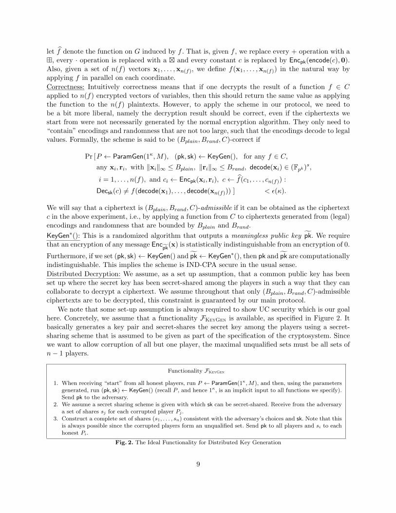
Theorem 3. The protocol ΠPREP (Figure 7) implements FPREP with computational security againstany static, active adversary corrupting up to n−1 parties, in the FKeyGen,FRand-hybrid model whenthe underlying cryptosystem is admissible6.

Protocol ReshareUsage: Input is em, where em = Encpk(m) is a public ciphertext and a parameter enc, where enc =

NewCiphertext or enc = NoNewCiphertext. Output is a share mi of m to each player Pi; and if enc =NewCiphertext, a ciphertext e′m. The idea is that em could be a product of two ciphertexts, which Reshareconverts to a “fresh” ciphertext e′m. Since Reshare uses distributed decryption (that may return an incorrectresult), it is not guaranteed that em and e′m contain the same value, but it is guaranteed that

∑imi is the

value contained in e′m.Reshare(em, enc) :

1. Each player Pi samples a uniform fi ∈ (Fpk )s. Define f :=∑ni=1 fi.

2. Each player Pi computes and broadcasts efi ← Encpk(fi).3. Each player Pi runs ΠZKPoPK acting as a prover on efi . The protocol aborts if any proof fails.4. The players compute ef ← ef1 · · · efn , and em+f ← em ef .5. The players invoke FKeyGenDec to decrypt em+f and thereby obtain m + f .6. P1 sets m1 ←m + f − f1, and each player Pi (i 6= 1) sets mi ← −fi.7. If enc = NewCiphertext, all players set e′m ← Encpk(m + f) ef1 · · · efn , where a default value for

the randomness is used when computing Encpk(m + f).

Fig. 4. The sub-protocol for additively secret sharing a plaintext m ∈ (Fpk )s on input a ciphertext em = Encpk(m).

Protocol PBracketUsage: On input shares v1, . . . ,vn privately held by the players and public ciphertext ev, this protocol generates

[[v]]. It is assumed that∑i vi is the plaintext contained in ev.

PBracket(v1, . . . ,vn, ev) :1. For i = 1, . . . , n

(a) All players set eγi ← eβiev (note that eβi is generated during the initialization process, and knownby every player)

(b) Players generate (γ1i , . . . γ

ni ) ← Reshare(eγi ,NoNewCiphertext), so each player Pj gets a share γji of

v · βi.2. Output the representation [[v]] = (v1, . . . ,vn, (βi, γ

i1, . . . , γ

in)i=1,...,n).

Fig. 5. The sub-protocol for generating [[v]].

Protocol PAngleUsage: On input shares v1, . . . ,vn privately held by the players and public ciphertext ev, this protocol generates〈v〉. It is assumed that

∑i vi is the plaintext contained in ev.

PAngle(v1, . . . ,vn, ev) :1. All players set ev·α ← ev eα (note that eα is generated during the initialization process, and known

by every player)2. Players generate (γ1, . . . , γn)← Reshare(ev·α,NoNewCiphertext), so each player Pi gets a share γi of α ·v.3. Output representation 〈v〉 = (0,v1, . . . ,vn, γ1, . . . , γn).

Fig. 6. The sub-protocol for generating 〈v〉.

6 The definition of admissible cryptosystem demands a decryption protocol that implements FKeyGenDec based onFKeyGen, hence the theorem only assumes FKeyGen.

12

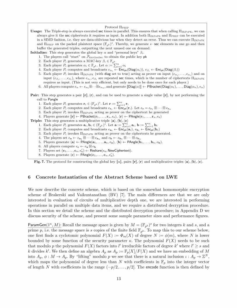
Protocol ΠPREP

Usage: The Triple-step is always executed sec times in parallel. This ensures that when calling ΠZKPoPK, we canalways give it the sec ciphertexts it requires as input. In addition both ΠZKPoPK and ΠPREP can be executedin a SIMD fashion, i.e. they are data-oblivious bar when they detect an error. Thus we can execute ΠZKPoPK

and ΠPREP on the packed plaintext space (Fpk )s. Thereby, we generate s · sec elements in one go and thenbuffer the generated triples, outputting the next unused one on demand.

Initialize: This step generates the global key α and “personal keys” βi.1. The players call “start” on FKeyGenDec to obtain the public key pk2. Each player Pi generates a MAC-key βi ∈ Fpk3. Each player Pi generates αi ∈ Fpk . Let α :=

∑ni=1 αi

4. Each player Pi computes and broadcasts eαi ← Encpk(Diag(αi)), eβi ← Encpk(Diag(βi))5. Each player Pi invokes ΠZKPoPK (with diag set to true) acting as prover on input (eαi , . . . , eαi) and on

input (eβi , . . . , eβi), where eαi , eβi are repeated sec times, which is the number of ciphertexts ΠZKPoPK

requires as input. (This is not very efficient, but only needs to be done once for each player.)6. All players compute eα ← eα1· · ·eαn , and generate [[Diag(α)]]← PBracket(Diag(α1), . . . ,Diag(αn), eα)

Pair: This step generates a pair [[r]], 〈r〉, and can be used to generate a single value [[r]], by not performing thecall to Pangle1. Each player Pi generates ri ∈ (Fpk )s. Let r :=

∑ni=1 ri

2. Each player Pi computes and broadcasts eri ← Encpk(ri). Let er = er1 · · · ern3. Each player Pi invokes ΠZKPoPK acting as prover on the ciphertext he generated4. Players generate [[r]]← PBracket(r1, . . . , rn, er), 〈r〉 ← PAngle(r1, . . . , rn, er)

Triple: This step generates a multiplicative triple 〈a〉, 〈b〉, 〈c〉1. Each player Pi generates ai,bi ∈ (Fpk )s. Let a :=

∑ni=1 ai, b :=

∑ni=1 bi

2. Each player Pi computes and broadcasts eai ← Encpk(ai), ebi ← Encpk(bi)3. Each player Pi invokes ΠZKPoPK acting as prover on the ciphertexts he generated.4. The players set ea ← ea1 · · · ean and eb ← eb1 · · · ebn

5. Players generate 〈a〉 ← PAngle(a1, . . . ,an, ea), 〈b〉 ← PAngle(b1, . . . ,bn, eb).6. All players compute ec ← ea eb7. Players set (c1, . . . , cn, e

′c)← Reshare(ec,NewCiphertext).

8. Players generate 〈c〉 ← PAngle(c1, . . . , cn, e′c).

Fig. 7. The protocol for constructing the global key [[α]], pairs [[r]], 〈r〉 and multiplicative triples 〈a〉, 〈b〉, 〈c〉.

6 Concrete Instantiation of the Abstract Scheme based on LWE

We now describe the concrete scheme, which is based on the somewhat homomorphic encryptionscheme of Brakerski and Vaikuntanathan (BV) [7]. The main differences are that we are onlyinterested in evaluation of circuits of multiplicative depth one, we are interested in performingoperations in parallel on multiple data items, and we require a distributed decryption procedure.In this section we detail the scheme and the distributed decryption procedure; in Appendix D wediscuss security of the scheme, and present some sample parameter sizes and performance figures.

ParamGen(1κ,M): Recall the message space is given by M = (Fpk)s for two integers k and s, and aprime p, i.e. the message space is s copies of the finite field Fpk . To map this to our scheme below,one first finds a cyclotomic polynomial F (X) := Φm(X) of degree N := φ(m), where N is lowerbounded by some function of the security parameter κ. The polynomial F (X) needs to be suchthat modulo p the polynomial F (X) factors into l′ irreducible factors of degree k′ where l′ ≥ s andk divides k′. We then define an algebra Ap as Ap := Fp[X]/F (X) and we have an embedding of Minto Ap, φ : M → Ap. By “lifting” modulo p we see that there is a natural inclusion ι : Ap → ZN ,which maps the polynomial of degree less than N with coefficients in Fp into the integer vectorof length N with coefficients in the range (−p/2, . . . , p/2]. The encode function is then defined by

13

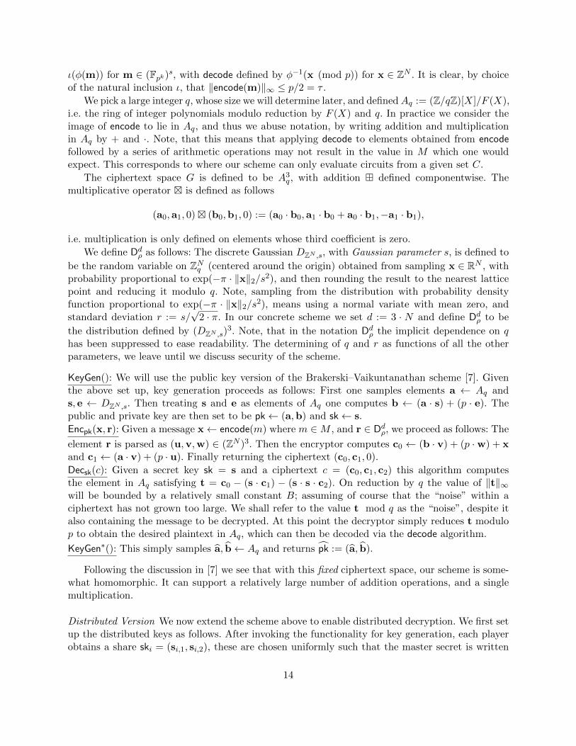
ι(φ(m)) for m ∈ (Fpk)s, with decode defined by φ−1(x (mod p)) for x ∈ ZN . It is clear, by choiceof the natural inclusion ι, that ‖encode(m)‖∞ ≤ p/2 = τ .

We pick a large integer q, whose size we will determine later, and definedAq := (Z/qZ)[X]/F (X),i.e. the ring of integer polynomials modulo reduction by F (X) and q. In practice we consider theimage of encode to lie in Aq, and thus we abuse notation, by writing addition and multiplicationin Aq by + and ·. Note, that this means that applying decode to elements obtained from encodefollowed by a series of arithmetic operations may not result in the value in M which one wouldexpect. This corresponds to where our scheme can only evaluate circuits from a given set C.

The ciphertext space G is defined to be A3q , with addition defined componentwise. The

multiplicative operator is defined as follows

(a0,a1, 0) (b0,b1, 0) := (a0 · b0,a1 · b0 + a0 · b1,−a1 · b1),

i.e. multiplication is only defined on elements whose third coefficient is zero.

We define Ddρ as follows: The discrete Gaussian DZN ,s, with Gaussian parameter s, is defined to

be the random variable on ZNq (centered around the origin) obtained from sampling x ∈ RN , withprobability proportional to exp(−π · ‖x‖2/s2), and then rounding the result to the nearest latticepoint and reducing it modulo q. Note, sampling from the distribution with probability densityfunction proportional to exp(−π · ‖x‖2/s2), means using a normal variate with mean zero, andstandard deviation r := s/

√2 · π. In our concrete scheme we set d := 3 · N and define Ddρ to be

the distribution defined by (DZN ,s)3. Note, that in the notation Ddρ the implicit dependence on q

has been suppressed to ease readability. The determining of q and r as functions of all the otherparameters, we leave until we discuss security of the scheme.

KeyGen(): We will use the public key version of the Brakerski–Vaikuntanathan scheme [7]. Giventhe above set up, key generation proceeds as follows: First one samples elements a ← Aq ands, e ← DZN ,s. Then treating s and e as elements of Aq one computes b ← (a · s) + (p · e). Thepublic and private key are then set to be pk← (a,b) and sk← s.

Encpk(x, r): Given a message x← encode(m) where m ∈M , and r ∈ Ddρ, we proceed as follows: The

element r is parsed as (u,v,w) ∈ (ZN )3. Then the encryptor computes c0 ← (b · v) + (p ·w) + xand c1 ← (a · v) + (p · u). Finally returning the ciphertext (c0, c1, 0).

Decsk(c): Given a secret key sk = s and a ciphertext c = (c0, c1, c2) this algorithm computesthe element in Aq satisfying t = c0 − (s · c1) − (s · s · c2). On reduction by q the value of ‖t‖∞will be bounded by a relatively small constant B; assuming of course that the “noise” within aciphertext has not grown too large. We shall refer to the value t mod q as the “noise”, despite italso containing the message to be decrypted. At this point the decryptor simply reduces t modulop to obtain the desired plaintext in Aq, which can then be decoded via the decode algorithm.

KeyGen∗(): This simply samples a, b← Aq and returns pk := (a, b).

Following the discussion in [7] we see that with this fixed ciphertext space, our scheme is some-what homomorphic. It can support a relatively large number of addition operations, and a singlemultiplication.

Distributed Version We now extend the scheme above to enable distributed decryption. We first setup the distributed keys as follows. After invoking the functionality for key generation, each playerobtains a share ski = (si,1, si,2), these are chosen uniformly such that the master secret is written

14

as

s = s1,1 + · · ·+ sn,1, s · s = s1,2 + · · ·+ sn,2.

As remarked earlier this one-time setup procedure can be accomplished by standard UC-securemultiparty computation protocols such as that described in [5]. The following theorem is proved inAppendix A.6. It depends on the constant B defined above. In Appendix D we compute the valueof B when the input ciphertext is (Bplain, Brand, C)-admissible, and show how to choose parametersfor the cryptosystem such that the required bound on B is satisfied.

Theorem 4. In the FKeyGen-hybrid model, the protocol ΠDDec (Figure 8) implements FKeyGenDec

with statistical security against any static active adversary corrupting up to n − 1 parties if B +2sec ·B < q/2.

Protocol ΠDDec

Initialize: Each party Pi on being given the ciphertext c = (c0, c1, c2), and an upper bound B on the infinitynorm of t above, computes

vi ←c0 − (si,1 · c1)− (si,2 · c2) if i = 1−(si,1 · c1)− (si,2 · c2) if i 6= 1

and sets ti ← vi + p · ri where ri is a random element with infinity norm bounded by 2sec ·B/(n · p).Public Decryption: All the players are supposed to learn the message.

– Each party Pi broadcasts ti– All players compute t′ ← t1 + · · ·+ tn and obtain a message m′ ← decode(t′ mod p).

Private Decryption: Only player Pj is supposed to learn the message.– Each party Pi sends ti to Pj– Pj computes t′ ← t1 + · · ·+ tn and obtain a message m′ ← decode(t′ mod p).

Fig. 8. The distributed decryption protocol.

7 Acknowledgements

The first, second and fourth author acknowledge support from the Danish National Research Foun-dation and The National Science Foundation of China (under the grant 61061130540) for the Sino-Danish Center for the Theory of Interactive Computation, within which [part of] this work wasperformed; and also from the CFEM research center (supported by the Danish Strategic ResearchCouncil) within which part of this work was performed.

The third author was supported by the European Commission through the ICT Programmeunder Contract ICT-2007-216676 ECRYPT II and via an ERC Advanced Grant ERC-2010-AdG-267188-CRIPTO, by EPSRC via grant COED–EP/I03126X, the Defense Advanced Research ProjectsAgency (DARPA) and the Air Force Research Laboratory (AFRL) under agreement numberFA8750-11-2-0079, and by a Royal Society Wolfson Merit Award. The US Government is autho-rized to reproduce and distribute reprints for Government purposes notwithstanding any copyrightnotation hereon. The views and conclusions contained herein are those of the authors and shouldnot be interpreted as necessarily representing the official policies or endorsements, either expressedor implied, of DARPA, AFRL, the U.S. Government, the European Commission or EPSRC.

The authors would like to thank Robin Chapman, Henri Cohen and Rob Harley for variousdiscussions whilst this work was carried out.

15

References

1. S. Arora and R. Ge. New algorithms for learning in presence of errors. In L. Aceto, M. Henzinger, and J. Sgall,editors, ICALP (1), volume 6755 of Lecture Notes in Computer Science, pages 403–415. Springer, 2011.

2. G. Asharov, A. Jain, A. Lopez-Alt, E. Tromer, V. Vaikuntanathan, and D. Wichs. Multiparty computation withlow communication, computation and interaction via threshold fhe. In D. Pointcheval and T. Johansson, editors,EUROCRYPT, volume 7237 of Lecture Notes in Computer Science, pages 483–501. Springer, 2012.

3. D. Beaver. Efficient multiparty protocols using circuit randomization. In J. Feigenbaum, editor, CRYPTO,volume 576 of Lecture Notes in Computer Science, pages 420–432. Springer, 1991.

4. E. Ben-Sasson, S. Fehr, and R. Ostrovsky. Near-linear unconditionally-secure multiparty computation with adishonest minority. IACR Cryptology ePrint Archive, 2011:629, 2011.

5. R. Bendlin, I. Damgard, C. Orlandi, and S. Zakarias. Semi-homomorphic encryption and multiparty computation.In EUROCRYPT, pages 169–188, 2011.

6. Z. Brakerski, C. Gentry, and V. Vaikuntanathan. Fully homomorphic encryption without bootstrapping. Elec-tronic Colloquium on Computational Complexity (ECCC), 18:111, 2011.

7. Z. Brakerski and V. Vaikuntanathan. Fully homomorphic encryption from ring-lwe and security for key dependentmessages. In P. Rogaway, editor, CRYPTO, volume 6841 of Lecture Notes in Computer Science, pages 505–524.Springer, 2011.

8. R. Canetti, Y. Lindell, R. Ostrovsky, and A. Sahai. Universally composable two-party and multi-party securecomputation. In STOC, pages 494–503, 2002.

9. Y. Chen and P. Q. Nguyen. Bkz 2.0: Better lattice security estimates. In D. H. Lee and X. Wang, editors,ASIACRYPT, volume 7073 of Lecture Notes in Computer Science, pages 1–20. Springer, 2011.

10. R. Cramer, I. Damgard, and V. Pastro. On the amortized complexity of zero knowledge protocols for multiplica-tive relations. In ICITS, 2012. To appear.

11. I. Damgard, M. Keller, E. Larraia, C. Miles, and N. P. Smart. Implementing aes via an actively/covertly securedishonest-majority mpc protocol. IACR Cryptology ePrint Archive, 2012:262, 2012.

12. I. Damgard and J. B. Nielsen. Perfect hiding and perfect binding universally composable commitment schemeswith constant expansion factor. In M. Yung, editor, CRYPTO, volume 2442 of Lecture Notes in ComputerScience, pages 581–596. Springer, 2002.

13. I. Damgard and C. Orlandi. Multiparty computation for dishonest majority: From passive to active security atlow cost. In CRYPTO, pages 558–576, 2010.

14. N. Gama and P. Q. Nguyen. Predicting lattice reduction. In N. P. Smart, editor, EUROCRYPT, volume 4965of Lecture Notes in Computer Science, pages 31–51. Springer, 2008.

15. C. Gentry. Fully homomorphic encryption using ideal lattices. In M. Mitzenmacher, editor, STOC, pages 169–178.ACM, 2009.

16. C. Gentry, S. Halevi, and N. P. Smart. Fully homomorphic encryption with polylog overhead. In D. Pointchevaland T. Johansson, editors, EUROCRYPT, volume 7237 of Lecture Notes in Computer Science, pages 465–482.Springer, 2012.

17. Y. Ishai, E. Kushilevitz, R. Ostrovsky, and A. Sahai. Zero-knowledge from secure multiparty computation. InD. S. Johnson and U. Feige, editors, STOC, pages 21–30. ACM, 2007.

18. Y. Ishai, M. Prabhakaran, and A. Sahai. Founding cryptography on oblivious transfer - efficiently. In D. Wagner,editor, CRYPTO, volume 5157 of Lecture Notes in Computer Science, pages 572–591. Springer, 2008.

19. Y. Lindell. Highly-efficient universally-composable commitments based on the ddh assumption. In EUROCRYPT,pages 446–466, 2011.

20. R. Lindner and C. Peikert. Better key sizes (and attacks) for lwe-based encryption. In A. Kiayias, editor,CT-RSA, volume 6558 of Lecture Notes in Computer Science, pages 319–339. Springer, 2011.

21. V. Lyubashevsky. Fiat-shamir with aborts: Applications to lattice and factoring-based signatures. In M. Matsui,editor, ASIACRYPT, volume 5912 of Lecture Notes in Computer Science, pages 598–616. Springer, 2009.

22. V. Lyubashevsky, C. Peikert, and O. Regev. On ideal lattices and learning with errors over rings. 2011.Manuscript.

23. D. Micciancio and O. Regev. Lattice-based cryptography, 2008.24. S. Myers, M. Sergi, and abhi shelat. Threshold fully homomorphic encryption and secure computation. IACR

Cryptology ePrint Archive, 2011:454, 2011.25. J. B. Nielsen, P. S. Nordholt, C. Orlandi, and S. S. Burra. A new approach to practical active-secure two-party

computation. IACR Cryptology ePrint Archive, 2011:91, 2011.26. M. Puschel and J. M. F. Moura. Algebraic signal processing theory: Cooley-tukey type algorithms for dcts and

dsts. IEEE Transactions on Signal Processing, 56(4):1502–1521, 2008.

16

27. N. P. Smart and F. Vercauteren. Fully homomorphic simd operations. IACR Cryptology ePrint Archive, 2011:133,2011.

28. S. Winkler and J. Wullschleger. On the efficiency of classical and quantum oblivious transfer reductions. InCRYPTO, pages 707–723, 2010.

A Proofs

A.1 Zero-Knowledge Proof

Construction of the Protocol. We will give two versions of the protocol. The first is a standard3-move protocol, the second uses an “abort” technique to optimize the parameter values, this oneis best suited for use with the Fiat-Shamir heuristic, and may be the best option for a practicalimplementation.

For the protocol, we will need that τ = p/2, so that ‖encode(m)‖∞ ≤ τ = p/2. This means thateach entry in encode(m) corresponds to a uniquely determined residue mod p (or equivalently anelement in Zp) and conversely each such residue is uniquely determined by m. We did not ask forthis in the abstract description, but the concrete instantiation satisfies this. Note that one problemwe need to address in the protocol is that not all vectors in the input domain of decode will giveus results in Fpk . However, if an input is equivalent mod p to encode(m) for some m then this isindeed the case, since then decode will return m. Therefore the verifier explicitly checks whetherthe encodings the prover sends him decode to legal values, this will imply that the ciphertexts inquestion also decode to legal values.

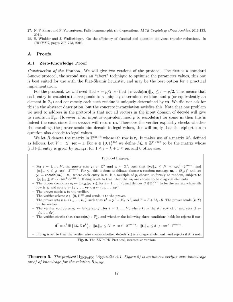
We let R denote the matrix in Zsec×d whose ith row is ri. It makes use of a matrix Me definedas follows. Let V := 2 · sec − 1. For e ∈ 0, 1sec we define Me ∈ ZV×sec to be the matrix whose(i, k)-th entry is given by ei−k+1, for 1 ≤ i− k + 1 ≤ sec and 0 otherwise.

Protocol ΠZKPoPK

– For i = 1, . . . , V , the prover sets yi ← ZN and si ← Zd, such that ‖yi‖∞ ≤ N · τ · sec2 · 2νsec−1 and‖si‖∞ ≤ d · ρ · sec2 · 2νsec−1. For yi, this is done as follows: choose a random message mi ∈ (Fpk )s and setyi = encode(mi) + ui, where each entry in ui is a multiple of p, chosen uniformly at random, subject to‖yi‖∞ ≤ N · τ · sec2 · 2νsec−1. If diag is set to true, then the mi are chosen to be diagonal elements.

– The prover computes ai ← Encpk(yi, si), for i = 1, . . . , V , and defines S ∈ ZV×d to be the matrix whose ithrow is si and sets y← (y1, . . . ,yV ), a← (a1, . . . , aV ).

– The prover sends a to the verifier.– The verifier selects e ∈ 0, 1sec and sends it to the prover.– The prover sets z← (z1, . . . , zV ), such that zT = yT +Me ·xT, and T = S+Me ·R. The prover sends (z, T )

to the verifier.– The verifier computes di ← Encpk(zi, ti), for i = 1, . . . , V , where ti is the ith row of T and sets d ←

(d1, . . . , dV ).– The verifier checks that decode(zi) ∈ Fspk and whether the following three conditions hold; he rejects if not

dT = aT (Me cT

), ‖zi‖∞ ≤ N · τ · sec2 · 2νsec−1, ‖ti‖∞ ≤ d · ρ · sec2 · 2νsec−1.

– If diag is set to true the verifier also checks whether decode(zi) is a diagonal element, and rejects if it is not.

Fig. 9. The ZKPoPK Protocol, interactive version.

Theorem 5. The protocol ΠZKPoPK (Appendix A.1, Figure 9) is an honest-verifier zero-knowledgeproof of knowledge for the relation RPoPK .

17

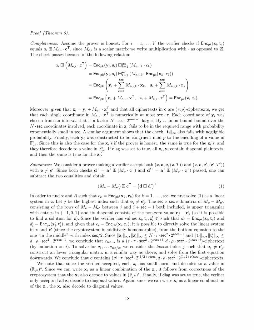
Proof (Theorem 5).

Completeness: Assume the prover is honest. For i = 1, . . . , V the verifier checks if Encpk(zi, ti)equals ai Me,i · cT, since Me,i is a scalar matrix we write multiplication with · as opposed to .The check passes because of the following relation:

ai (Me,i · cT

)= Encpk(yi, si)

seck=1 (Me,i,k · ck)

= Encpk(yi, si) seck=1 (Me,i,k · Encpk(xk, rk))

= Encpk

(yi +

sec∑k=1

Me,i,k · xk, si +sec∑k=1

Me,i,k · rk

)= Encpk

(yi +Me,i · xT, si +Me,i · rT

)= Encpk(zi, ti).

Moreover, given that zi = yi +Me,i · xT and that all ciphertexts in c are (τ, ρ)-ciphertexts, we getthat each single coordinate in Me,i · xT is numerically at most sec · τ . Each coordinate of yi waschosen from an interval that is a factor N · sec · 2νsec−1 larger. By a union bound bound over theN · sec coordinates involved, each coordinate in zi fails to be in the required range with probabilityexponentially small in sec. A similar argument shows that the check ‖ti‖∞ also fails with negligibleprobability. Finally, each yi was constructed to be congruent mod p to the encoding of a value inFspk

. Since this is also the case for the xi’s if the prover is honest, the same is true for the zi’s, andthey therefore decode to a value in Fs

pk. If diag was set to true, all xi,yi contain diagonal plaintexts,

and then the same is true for the zi.

Soundness: We consider a prover making a verifier accept both (x,a, e, (z, T )) and (x,a, e′, (z′, T ′))with e 6= e′. Since both checks dT = aT (Me · cT) and d′T = aT (Me′ · cT) passed, one cansubtract the two equalities and obtain

(Me −Me′) cT =(d d′

)T(1)

In order to find x and R such that ck = Encpk(xk, rk) for k = 1, . . . , sec, we first solve (1) as a linearsystem in c. Let j be the highest index such that ej 6= e′j . The sec × sec submatrix of Me −Me′ ,consisting of the rows of Me −Me′ between j and j + sec − 1 both included, is upper triangularwith entries in −1, 0, 1 and its diagonal consists of the non-zero value ej − e′j (so it is possibleto find a solution for c). Since the verifier has values zi, ti, z

′i, t′i such that di = Encpk(zi, ti) and

d′i = Encpk(z′i, t′i), and given that ci = Encpk(xi, ri), it is possible to directly solve the linear system

in x and R (since the cryptosystem is additively homomorphic), from the bottom equation to theone “in the middle” with index sec/2. Since ‖zi‖∞, ‖z′i‖∞ ≤ N · τ · sec2 ·2νsec−1 and ‖ti‖∞, ‖t′i‖∞ ≤d · ρ · sec2 · 2νsec−1, we conclude that csec−i is a (s · τ · sec2 · 2νsec+i, d · ρ · sec2 · 2νsec+i)-ciphertext(by induction on i). To solve for c1, . . . csec/2, we consider the lowest index j such that ej 6= e′j ,construct an lower triangular matrix in a similar way as above, and solve from the first equationdownwards. We conclude that c contains (N · τ · sec2 · 2(1/2+ν)sec, d · ρ · sec2 · 2(1/2+ν)sec)-ciphertexts.

We note that since the verifier accepted, each zi has small norm and decodes to a value in(Fpk)s. Since we can write xi as a linear combination of the zi, it follows from correctness of thecryptosystem that the xi also decode to values in (Fpk)s. Finally, if diag was set to true, the verifieronly accepts if all zi decode to diagonal values. Again, since we can write xi as a linear combinationof the zi, the xi also decode to diagonal values.

18

Zero-Knowledge: We give an honest-verifier simulator for the protocol that outputs accepting con-versations. In order to simulate one repetition, the simulator samples e ∈ 0, 1sec uniformly andz, T uniformly with the constrain that d contains random ciphertexts satisfying the verifiers check,i.e., zi, ti are uniform, subject to ‖zi‖∞ ≤ N ·τ ·sec2 ·2νsec−1, ‖ti‖∞ ≤ d·ρ·sec2 ·2νsec−1, where more-over zi is generated as encode(mi)+ui where mi is a random plaintext (diagonal if diag is set to true)and ui contains multiples of p that are uniformly random, subject to ‖zi‖∞ ≤ N · τ · sec2 · 2νsec−1.Finally, a is computed as aT ← dT (Me · cT). In the real conversation, the provers choice ofvalues in zi and ti are statistically close to the distribution used by the simulator. This is becausethe prover uses the same method to generate these values, except that he adds in some vectorsof exponentially smaller norm which leads to a statistically close distribution. Since e has thecorrect distribution and a follows deterministically from the last two messages, the simulation isstatistically indistinguishable.

ut

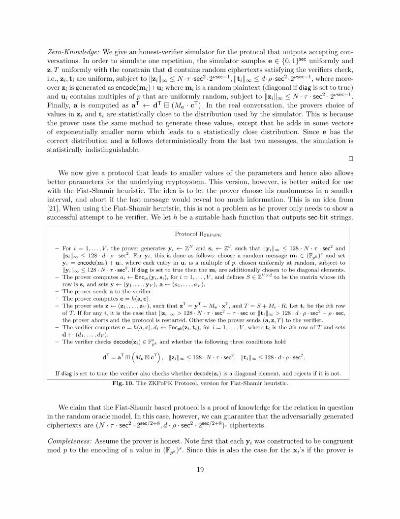
We now give a protocol that leads to smaller values of the parameters and hence also allowsbetter parameters for the underlying cryptoystem. This version, however, is better suited for usewith the Fiat-Shamir heuristic. The idea is to let the prover choose his randomness in a smallerinterval, and abort if the last message would reveal too much information. This is an idea from[21]. When using the Fiat-Shamir heuristic, this is not a problem as he prover only needs to show asuccessful attempt to he verifier. We let h be a suitable hash function that outputs sec-bit strings.

Protocol ΠZKPoPK

– For i = 1, . . . , V , the prover generates yi ← ZN and si ← Zd, such that ‖yi‖∞ ≤ 128 · N · τ · sec2 and‖si‖∞ ≤ 128 · d · ρ · sec2. For yi, this is done as follows: choose a random message mi ∈ (Fpk )s and setyi = encode(mi) + ui, where each entry in ui is a multiple of p, chosen uniformly at random, subject to‖yi‖∞ ≤ 128 ·N · τ · sec2. If diag is set to true then the mi are additionally chosen to be diagonal elements.

– The prover computes ai ← Encpk(yi, si), for i = 1, . . . , V , and defines S ∈ ZV×d to be the matrix whose ithrow is si and sets y← (y1, . . . ,yV ), a← (a1, . . . , aV ).

– The prover sends a to the verifier.– The prover computes e = h(a, c).– The prover sets z← (z1, . . . , zV ), such that zT = yT +Me · xT, and T = S +Me · R. Let ti be the ith row

of T . If for any i, it is the case that ‖zi‖∞ > 128 ·N · τ · sec2 − τ · sec or ‖ti‖∞ > 128 · d · ρ · sec2 − ρ · sec,the prover aborts and the protocol is restarted. Otherwise the prover sends (a, z, T ) to the verifier.

– The verifier computes e = h(a, c), di ← Encpk(zi, ti), for i = 1, . . . , V , where ti is the ith row of T and setsd← (d1, . . . , dV ).

– The verifier checks decode(zi) ∈ Fspk and whether the following three conditions hold

dT = aT (Me cT

), ‖zi‖∞ ≤ 128 ·N · τ · sec2, ‖ti‖∞ ≤ 128 · d · ρ · sec2.

If diag is set to true the verifier also checks whether decode(zi) is a diagonal element, and rejects if it is not.

Fig. 10. The ZKPoPK Protocol, version for Fiat-Shamir heuristic.

We claim that the Fiat-Shamir based protocol is a proof of knowledge for the relation in questionin the random oracle model. In this case, however, we can guarantee that the adversarially generatedciphertexts are (N · τ · sec2 · 2sec/2+8, d · ρ · sec2 · 2sec/2+8)- ciphertexts.

Completeness: Assume the prover is honest. Note first that each yi was constructed to be congruentmod p to the encoding of a value in (Fpk)s. Since this is also the case for the xi’s if the prover is

19

honest, the same is true for the zi’s, and they therefore always decode to a value in (Fpk)s. If diagwas set to true, all xi,yi contain diagonal plaintexts, and then the same is true for the zi.

Next, for i = 1, . . . , V the verifier checks if Encpk(zi, ti) equals aiMe,i ·cT, since Me,i is a scalarmatrix we write multiplication with · as opposed to . The check passes because of the followingrelation:

ai (Me,i · cT

)= Encpk(yi, si)

seck=1 (Me,i,k · ck)

= Encpk(yi, si) seck=1 (Me,i,k · Encpk(xk, rk))

= Encpk

(yi +

sec∑k=1

Me,i,k · xk, si +

sec∑k=1

Me,i,k · rk

)= Encpk

(yi +Me,i · xT, si +Me,i · rT

)= Encpk(zi, ti).

Moreover, given that zi = yi +Me,i · xT and that all ciphertexts in c are (τ, ρ)-ciphertexts, we getthat each single coordinate in Me,i · xT is numerically at most sec · τ . Each coordinate of yi waschosen from an interval that is a factor 128 · N · sec larger. Therefore each coordinate in zi failsto be in the required range with probability 1/(128 · N · sec). Note that this probability does notdepend on the concrete values of the coordinates in Me,i · xT, only on the bound on the numericvalue.

By a union bound over the N coordinates of zi we get that ‖zi‖∞ ≤ 128 ·N ·τ · sec2−τ · sec failswith probability at most 1/(128 ·sec), and by a final union bound over the 2 sec−1 ciphtertexts thatall checks on the zi’s are ok except with probability at most 1/64. A similar argument shows thatthe check ‖ti‖∞ ≤ 128 · d · ρ · sec2 − ρ · sec fails also with probability at most 1/64. The conclusionis that the prover will abort with probability at most 1/32, so we expect to only have to repeat theprotocol once to have success.

Soundness: By a standard argument, a prover who can efficiently produce a valid proof is able toproduce (x,a, e, (z, T )) and (x,a, e′, (z′, T ′)) with e 6= e′ that the verifier would accept. Since bothchecks dT = aT (Me · cT) and d′T = aT (Me′ · cT) passed, one can subtract the two equalitiesand obtain

(Me −Me′) cT =(d d′

)T(2)

In order to find x and R such that ck = Encpk(xk, rk) for k = 1, . . . , sec, we first solve (2) as a linearsystem in c. Let j be the highest index such that ej 6= e′j . The sec × sec submatrix of Me −Me′ ,consisting of the rows of Me −Me′ between j and j + sec − 1 both included, is upper triangularwith entries in −1, 0, 1 and its diagonal consists of the non-zero value ej − e′j (so it is possibleto find a solution for c). Since the verifier has values zi, ti, z

′i, t′i such that di = Encpk(zi, ti) and

d′i = Encpk(z′i, t′i), and given that ci = Encpk(xi, ri), it is possible to directly solve the linear system

in x and R (since the cryptosystem is additively homomorphic), from the bottom equation to theone “in the middle” with index sec/2.Since ‖zi‖∞, ‖z′i‖∞ ≤ 128 ·N · τ · sec2 and ‖ti‖∞, ‖t′i‖∞ ≤ 128 · d · ρ · sec2, we conclude that csec−imust be a (256 · N · τ · 2i · sec2, 256 · d · ρ · 2i · sec2)-ciphertext (by induction on i). To solve forc1, . . . csec/2, we consider the lowest index j such that ej 6= e′j , construct an lower triangular matrixin a similar way as above, and solve from the first equation downwards. We conclude that c contains(N · τ · sec2 · 2sec/2+8, d · ρ · sec2 · 2sec/2+8)-ciphertexts.

20

We note that since the verifier accepted, each zi has small norm and decodes to a value in(Fpk)s. Since we can write xi as a linear combination of the zi, it follows from correctness of thecryptosystem that the xi also decode to values (Fpk)s. Finally, if diag was set to true, the verifieronly accepts if all zi decode to diagonal values. Again, since we can write xi as a linear combinationof the zi, the xi also decode to diagonal values.

Zero-Knowledge: We give an honest-verifier simulator for the protocol that outputs an acceptingconversation (that does not abort).

In order to simulate one repetition, the simulator samples e ∈ 0, 1sec uniformly and z, Tuniformly with the constrain that d contains random (8 ·N · τ · sec2− τ · sec, 8 · d · ρ · sec2− ρ · sec)-ciphertexts. where moreover zi is generated as encode(mi) + ui where mi is a random plaintext(a diagonal one if diag is set to true) and ui contains multiples of p that are uniformly random,subject to ‖zi‖∞ ≤ 8N · τ · sec2− τ · sec. Finally, a is computed as aT ← dT (Me · cT). Define therandom oracle to output e on input a, c, output (a, e, (z, T )) and stop.

We argue that this simulation is perfect: The distribution of a simulated e is the same as a realone. Also, it is straightforward to see that in a real conversation, given that the prover does notabort, the vectors zi, ti will be uniformly random, subject to ‖zi‖∞ ≤ 8 · s · τ · sec2 − τ · sec and‖ti‖∞ ≤ 8 · d · ρ · sec2 − ρ · sec. So the simulator chooses zi, ti with exactly the right distribution.Since the value of a follows deterministically from the e, zi, ti, we have what we wanted.

Doing without random oracles. The above protocol can also be executed without using the Fiat-Shamir heuristic. In this case, the prover will start sec/5 instances of the protocol, computinga1, . . . ,asec/5. We choose this number of instance because it will ensure that the prover fails on all

of them with probability only (1/32)sec/5 = 2−sec. The prover commits to all these values, whichcan be done, for instance, with a Merkle hash tree, in which case the commitment will be veryshort, and any of a’s can be opened by sending a piece of information that is only logarithmic insec.

The verifier selects e, the prover finds an instance where he would not abort the protocol withthis e, opens the corresponding a and completes that instance.

This is complete and zero-knowledge by the same argument as above plus the hiding propertyof the commitment scheme used. Soundness follows from the fact that if the prover succeeds withprobability significantly greater that 2−sec · sec/5 he must be able to answer different challengescorrectly for some fixed instance out of the sec/5 we have. Such answers can be extracted byrewinding, and then the rest of the argument is the same as above.

A.2 The UC Model

In the following sections, we show that the online and preprocessing phases of our protocol aresecure in the UC model. We briefly recall how this model works: we will use the variant where thereis only one adversarial entity, the environment Z. The environment chooses inputs for the honestplayers and gets their outputs when the protocol is done. It also does an attack on the protocolwhich is our case means that it corrupts up to n − 1 of the players and takes control over theiractions. When Z stops, it outputs a bit. This process where Z interacts with the real players andprotocol is called the real process.

To define what it means that the protocol implements functionality F securely we assume thereexists a simulator S that interacts with both F and Z. Towards F , it chooses inputs for the corrupt

21

players and will get their outputs. Towards Z, it must simulate a view of the protocol that lookslike what Z would see in a real attack. This process is called the ideal process, and here F suppliesZ with the i/o interface of honest players. We say that the protocol implements F securely if Zoutputs 1 with essentially the same probability in the real as in the ideal process. We speak ofcomputational security if Z is assumed to be poly-time bounded and of statistical security if Z isunbounded.

A.3 Online Phase

On generating the ei’s Before proving the online protocol UC secure, we compute the probabilityof getting away with cheating in step 4 of ‘Output’ and how this depends on the way we generatethe ei’s.

For this purpose we design the following security game:

1. The challenger generates the secret key α and MACs γi ← αmi and sends messages m1, . . . ,mT

to the adversary.2. The adversary sends back messages m′1, . . . ,m

′T .

3. The challenger generates random values e1, . . . , eT ← Fpk and sends them to the adversary.4. The adversary provides an error ∆.5. Set m←

∑Ti=0 eim

′i, γ ←

∑Ti=0 eiγi. Now, the challenger checks that αm = γ +∆

The adversary wins the game if there is an i for which m′i 6= mi and the final check goes through.It is not difficult to see that this game indeed models ‘Output’(up to step 4): The second step

in the game where the adversary sends the m′i’s models the fact that corrupted players can chooseto lie about their shares of values opened during the protocol execution. ∆ models the fact thatthe adversary is allowed to introduce errors on the macs when data are sent to FPREP in the initialpart of the protocol and may also modify the shares of macs held by corrupt players. Finally, sinceα, γ are secret shared in the protocol, the adversary has no information on α, γ ahead of time inthe protocol, just as in the security game.

Now, let us look at the probability of winning the game if the ei’s are randomly chosen. Ifthe check goes through, we have that the following equality holds: α

∑Ti=0 ei(m

′i −mi) = ∆. First

we consider the case where∑T

i=0 ei(m′i − mi) 6= 0, so α = ∆/

∑Ti=0 ei(m

′i − mi). This implies

that being able to pass the check is equivalent to guessing α. However, since the adversary has noinformation about α, this happens with probability only 1/|Fpk |. So what is left is to argue that∑T

i=0 ei(m′i − mi) = 0 also happens with very low probability. This can be seen as follows. We

define µi := (m′i − mi) and µ := (µ1, . . . , µT ), e := (e1, . . . , eT ). Now fµ(e) := e · µ =∑T

i=0 eiµidefines a linear mapping, which is not the 0-mapping since at least one µi 6= 0. From linear algebrawe then have the rank-nullity theorem telling us that dim(ker(fµ)) = T − 1. Also since e is randomand the adversary does not know e when choosing the m′i’s, the probability of e ∈ ker(fµ) is|FT−1pk|/|FT

pk| = 1/|Fpk |. Summing up, the total probability of winning the game is at most 2/|Fpk |.

Since choosing the ei’s uniformly would require an expensive coin-flip protocol, we use a differentway to generate them in the protocol: namely e1 is chosen at random and for i > 1, ei ← ei1.This has the advantage of adding only a constant number of multiplications in Fpk for a secure

multiplication. On the security side, we still want that∑T

i=0 eiµi = 0 should happen with smallprobability. Viewing fµ as a polynomial of degree T , we know it has at most T roots, so we haveto make sure we have an upper bound on T such that e1 is chosen from a field big enough for T/pk

to be negligible.

22

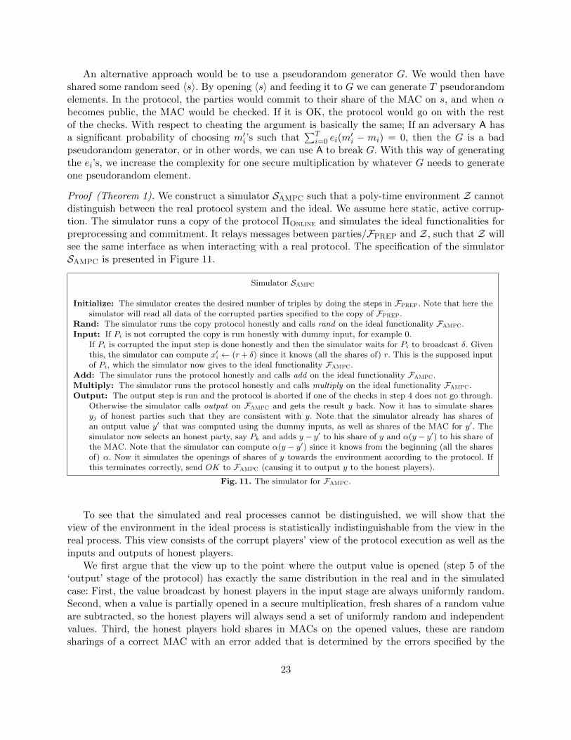
An alternative approach would be to use a pseudorandom generator G. We would then haveshared some random seed 〈s〉. By opening 〈s〉 and feeding it to G we can generate T pseudorandomelements. In the protocol, the parties would commit to their share of the MAC on s, and when αbecomes public, the MAC would be checked. If it is OK, the protocol would go on with the restof the checks. With respect to cheating the argument is basically the same; If an adversary A hasa significant probability of choosing m′i’s such that

∑Ti=0 ei(m

′i − mi) = 0, then the G is a bad

pseudorandom generator, or in other words, we can use A to break G. With this way of generatingthe ei’s, we increase the complexity for one secure multiplication by whatever G needs to generateone pseudorandom element.

Proof (Theorem 1). We construct a simulator SAMPC such that a poly-time environment Z cannotdistinguish between the real protocol system and the ideal. We assume here static, active corrup-tion. The simulator runs a copy of the protocol ΠOnline and simulates the ideal functionalities forpreprocessing and commitment. It relays messages between parties/FPREP and Z, such that Z willsee the same interface as when interacting with a real protocol. The specification of the simulatorSAMPC is presented in Figure 11.

Simulator SAMPC

Initialize: The simulator creates the desired number of triples by doing the steps in FPREP. Note that here thesimulator will read all data of the corrupted parties specified to the copy of FPREP.

Rand: The simulator runs the copy protocol honestly and calls rand on the ideal functionality FAMPC.Input: If Pi is not corrupted the copy is run honestly with dummy input, for example 0.

If Pi is corrupted the input step is done honestly and then the simulator waits for Pi to broadcast δ. Giventhis, the simulator can compute x′i ← (r+ δ) since it knows (all the shares of) r. This is the supposed inputof Pi, which the simulator now gives to the ideal functionality FAMPC.

Add: The simulator runs the protocol honestly and calls add on the ideal functionality FAMPC.Multiply: The simulator runs the protocol honestly and calls multiply on the ideal functionality FAMPC.Output: The output step is run and the protocol is aborted if one of the checks in step 4 does not go through.

Otherwise the simulator calls output on FAMPC and gets the result y back. Now it has to simulate sharesyj of honest parties such that they are consistent with y. Note that the simulator already has shares ofan output value y′ that was computed using the dummy inputs, as well as shares of the MAC for y′. Thesimulator now selects an honest party, say Pk and adds y− y′ to his share of y and α(y− y′) to his share ofthe MAC. Note that the simulator can compute α(y − y′) since it knows from the beginning (all the sharesof) α. Now it simulates the openings of shares of y towards the environment according to the protocol. Ifthis terminates correctly, send OK to FAMPC (causing it to output y to the honest players).

Fig. 11. The simulator for FAMPC.

To see that the simulated and real processes cannot be distinguished, we will show that theview of the environment in the ideal process is statistically indistinguishable from the view in thereal process. This view consists of the corrupt players’ view of the protocol execution as well as theinputs and outputs of honest players.

We first argue that the view up to the point where the output value is opened (step 5 of the‘output’ stage of the protocol) has exactly the same distribution in the real and in the simulatedcase: First, the value broadcast by honest players in the input stage are always uniformly random.Second, when a value is partially opened in a secure multiplication, fresh shares of a random valueare subtracted, so the honest players will always send a set of uniformly random and independentvalues. Third, the honest players hold shares in MACs on the opened values, these are randomsharings of a correct MAC with an error added that is determined by the errors specified by the

23

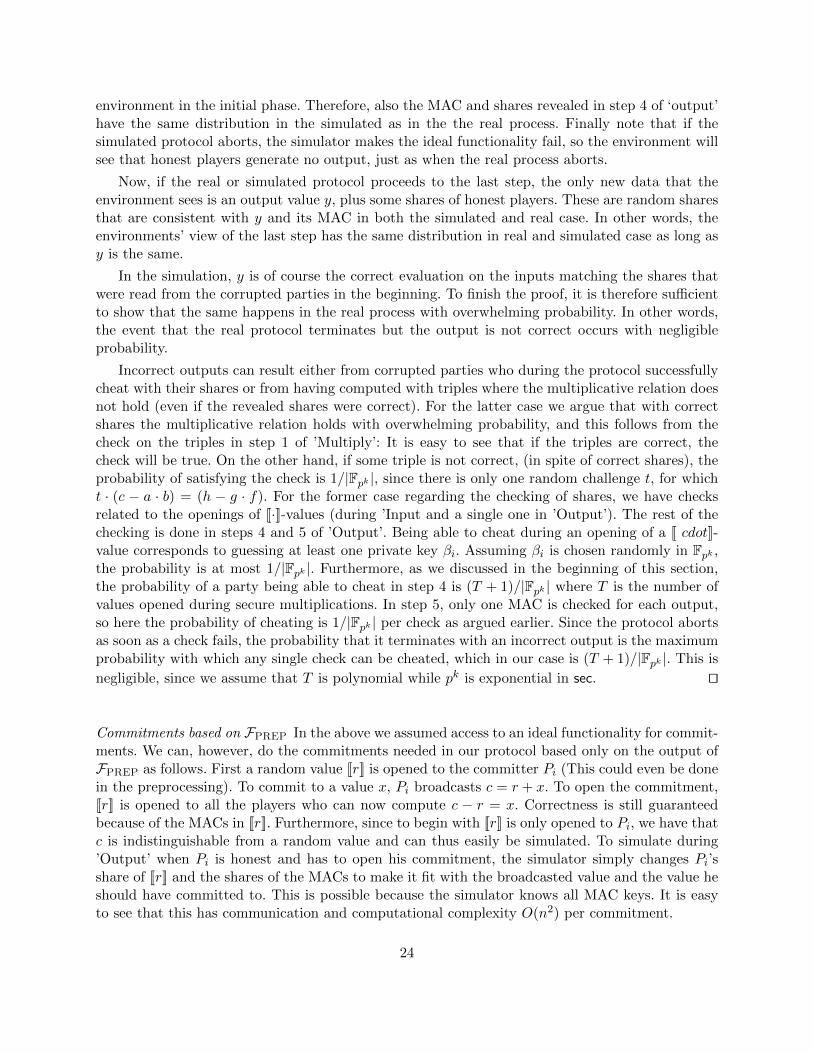
environment in the initial phase. Therefore, also the MAC and shares revealed in step 4 of ‘output’have the same distribution in the simulated as in the the real process. Finally note that if thesimulated protocol aborts, the simulator makes the ideal functionality fail, so the environment willsee that honest players generate no output, just as when the real process aborts.

Now, if the real or simulated protocol proceeds to the last step, the only new data that theenvironment sees is an output value y, plus some shares of honest players. These are random sharesthat are consistent with y and its MAC in both the simulated and real case. In other words, theenvironments’ view of the last step has the same distribution in real and simulated case as long asy is the same.

In the simulation, y is of course the correct evaluation on the inputs matching the shares thatwere read from the corrupted parties in the beginning. To finish the proof, it is therefore sufficientto show that the same happens in the real process with overwhelming probability. In other words,the event that the real protocol terminates but the output is not correct occurs with negligibleprobability.

Incorrect outputs can result either from corrupted parties who during the protocol successfullycheat with their shares or from having computed with triples where the multiplicative relation doesnot hold (even if the revealed shares were correct). For the latter case we argue that with correctshares the multiplicative relation holds with overwhelming probability, and this follows from thecheck on the triples in step 1 of ’Multiply’: It is easy to see that if the triples are correct, thecheck will be true. On the other hand, if some triple is not correct, (in spite of correct shares), theprobability of satisfying the check is 1/|Fpk |, since there is only one random challenge t, for whicht · (c − a · b) = (h − g · f). For the former case regarding the checking of shares, we have checksrelated to the openings of [[·]]-values (during ’Input and a single one in ’Output’). The rest of thechecking is done in steps 4 and 5 of ’Output’. Being able to cheat during an opening of a [[ cdot]]-value corresponds to guessing at least one private key βi. Assuming βi is chosen randomly in Fpk ,the probability is at most 1/|Fpk |. Furthermore, as we discussed in the beginning of this section,the probability of a party being able to cheat in step 4 is (T + 1)/|Fpk | where T is the number ofvalues opened during secure multiplications. In step 5, only one MAC is checked for each output,so here the probability of cheating is 1/|Fpk | per check as argued earlier. Since the protocol abortsas soon as a check fails, the probability that it terminates with an incorrect output is the maximumprobability with which any single check can be cheated, which in our case is (T + 1)/|Fpk |. This is

negligible, since we assume that T is polynomial while pk is exponential in sec. ut

Commitments based on FPREP In the above we assumed access to an ideal functionality for commit-ments. We can, however, do the commitments needed in our protocol based only on the output ofFPREP as follows. First a random value [[r]] is opened to the committer Pi (This could even be donein the preprocessing). To commit to a value x, Pi broadcasts c = r + x. To open the commitment,[[r]] is opened to all the players who can now compute c − r = x. Correctness is still guaranteedbecause of the MACs in [[r]]. Furthermore, since to begin with [[r]] is only opened to Pi, we have thatc is indistinguishable from a random value and can thus easily be simulated. To simulate during’Output’ when Pi is honest and has to open his commitment, the simulator simply changes Pi’sshare of [[r]] and the shares of the MACs to make it fit with the broadcasted value and the value heshould have committed to. This is possible because the simulator knows all MAC keys. It is easyto see that this has communication and computational complexity O(n2) per commitment.

24

Implementing Broadcast and Multiple Inputs/Outputs To implement broadcast based on point-to-point channels, we first observe that since we do not guarantee termination anyway, the broadcastdoes not have to terminate either. Therefore the following very simple protocol for broadcastingx ∈ Fpk is sufficient:

1. The broadcaster sends x to all players.2. Each player sends to all players what he received in the previous step.3. Each player checks that he received the value x from all players. If, so output x, otherwise abort.

This protocol has communication complexity O(n2) field elements for one broadcast. However,this can be optimized in case we need to broadcast many values. Below, we assume each playersends one value, say Pi wants to send xi. We also assume that we have a random value [[s]] from thepreprocessing, and that we have an ε-almost universal class of hash functions hs for negligible ε,indexed by values s, taking as input strings of n elements in Fpk and producing output in Fpk . Asimple example is where we view the input F as specifying coefficients of a polynomial of degreen−1, and hs(F ) is the result of evaluating this polynomial in point s. If two inputs F, F ′ are distinct,their difference has at most n− 1 roots, so the probability that hs(F ) = hs(F

′) is (n− 1)/pk. Theprotocol goes as follows:

1. Pi sends xi to all players.2. [[s]] is opened.3. Each player sends to all players hs(F ) where F is the string of values he received in the first

step.4. Each players checks that he received the same hash value from all players. If, so output x1, . . . , xn

as received in the first step, otherwise abort.

It is clear that if a player sent different data to different honest players, some honest player willabort, except with probability (n− 1)/pk. This protocol has complexity O(n2), including also thecost of opening [[s]]. But the cost per value we broadcast is only O(n). This protocol generalizeseasily to a case where one player has n values to broadcast.

In the online protocol we specified before, broadcast is used to give inputs in the first stage.Here, all players broadcast a value, and this is readily implemented with the optimized broadcastprotocol above, so we get complexity O(n) per input gate. If players have several inputs, we justexecute several instances of this broadcast.

The only other point where broadcast is used is in partial openings where a designated playerP1 broadcasts the value that is be to opened. Here, we can simply buffer the values sent until wehave n of them and then do the check in step 3-4 above that P1 has sent the same values to allplayers. Note that even if we allow P1 to send different data to different players for a while, thisdoes not allow information to leak: the fact observed in the simulation proof above, that in anypartial opening the honest players always send random independent values, still holds even if P1

has sent inconsistent data in previous rounds.

A.4 Running the online Phase with Small Fields

Suppose we want error probability 2−sec, and log pk is much smaller than sec.When we consider how to solve this problem, we will at first ignore Step 1 in the Multiply

stage on the online protocol, where one triple is “sacrificed” to check another, as this step could be

25

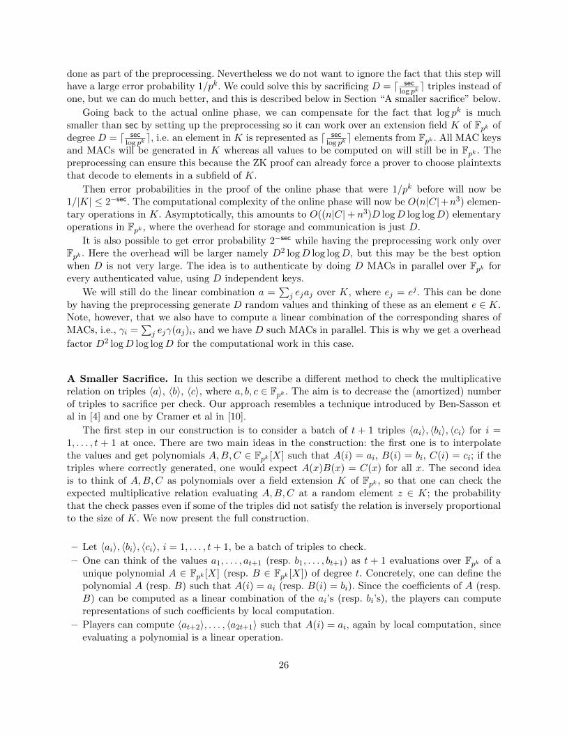
done as part of the preprocessing. Nevertheless we do not want to ignore the fact that this step willhave a large error probability 1/pk. We could solve this by sacrificing D = d sec

log pke triples instead of

one, but we can do much better, and this is described below in Section “A smaller sacrifice” below.

Going back to the actual online phase, we can compensate for the fact that log pk is muchsmaller than sec by setting up the preprocessing so it can work over an extension field K of Fpk ofdegree D = d sec

log pke, i.e. an element in K is represented as d sec

log pke elements from Fpk . All MAC keys

and MACs will be generated in K whereas all values to be computed on will still be in Fpk . Thepreprocessing can ensure this because the ZK proof can already force a prover to choose plaintextsthat decode to elements in a subfield of K.

Then error probabilities in the proof of the online phase that were 1/pk before will now be1/|K| ≤ 2−sec. The computational complexity of the online phase will now be O(n|C|+n3) elemen-tary operations in K. Asymptotically, this amounts to O((n|C|+ n3)D logD log logD) elementaryoperations in Fpk , where the overhead for storage and communication is just D.

It is also possible to get error probability 2−sec while having the preprocessing work only overFpk . Here the overhead will be larger namely D2 logD log logD, but this may be the best optionwhen D is not very large. The idea is to authenticate by doing D MACs in parallel over Fpk forevery authenticated value, using D independent keys.

We will still do the linear combination a =∑

j ejaj over K, where ej = ej . This can be doneby having the preprocessing generate D random values and thinking of these as an element e ∈ K.Note, however, that we also have to compute a linear combination of the corresponding shares ofMACs, i.e., γi =

∑j ejγ(aj)i, and we have D such MACs in parallel. This is why we get a overhead

factor D2 logD log logD for the computational work in this case.

A Smaller Sacrifice. In this section we describe a different method to check the multiplicativerelation on triples 〈a〉, 〈b〉, 〈c〉, where a, b, c ∈ Fpk . The aim is to decrease the (amortized) numberof triples to sacrifice per check. Our approach resembles a technique introduced by Ben-Sasson etal in [4] and one by Cramer et al in [10].

The first step in our construction is to consider a batch of t + 1 triples 〈ai〉, 〈bi〉, 〈ci〉 for i =1, . . . , t + 1 at once. There are two main ideas in the construction: the first one is to interpolatethe values and get polynomials A,B,C ∈ Fpk [X] such that A(i) = ai, B(i) = bi, C(i) = ci; if thetriples where correctly generated, one would expect A(x)B(x) = C(x) for all x. The second ideais to think of A,B,C as polynomials over a field extension K of Fpk , so that one can check theexpected multiplicative relation evaluating A,B,C at a random element z ∈ K; the probabilitythat the check passes even if some of the triples did not satisfy the relation is inversely proportionalto the size of K. We now present the full construction.

– Let 〈ai〉, 〈bi〉, 〈ci〉, i = 1, . . . , t+ 1, be a batch of triples to check.

– One can think of the values a1, . . . , at+1 (resp. b1, . . . , bt+1) as t + 1 evaluations over Fpk of aunique polynomial A ∈ Fpk [X] (resp. B ∈ Fpk [X]) of degree t. Concretely, one can define thepolynomial A (resp. B) such that A(i) = ai (resp. B(i) = bi). Since the coefficients of A (resp.B) can be computed as a linear combination of the ai’s (resp. bi’s), the players can computerepresentations of such coefficients by local computation.

– Players can compute 〈at+2〉, . . . , 〈a2t+1〉 such that A(i) = ai, again by local computation, sinceevaluating a polynomial is a linear operation.

26

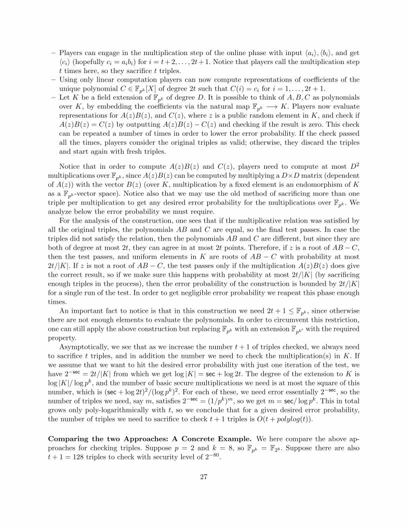
– Players can engage in the multiplication step of the online phase with input 〈ai〉, 〈bi〉, and get〈ci〉 (hopefully ci = aibi) for i = t+ 2, . . . , 2t+ 1. Notice that players call the multiplication stept times here, so they sacrifice t triples.

– Using only linear computation players can now compute representations of coefficients of theunique polynomial C ∈ Fpk [X] of degree 2t such that C(i) = ci for i = 1, . . . , 2t+ 1.

– Let K be a field extension of Fpk of degree D. It is possible to think of A,B,C as polynomialsover K, by embedding the coefficients via the natural map Fpk −→ K. Players now evaluaterepresentations for A(z)B(z), and C(z), where z is a public random element in K, and check ifA(z)B(z) = C(z) by outputting A(z)B(z)−C(z) and checking if the result is zero. This checkcan be repeated a number of times in order to lower the error probability. If the check passedall the times, players consider the original triples as valid; otherwise, they discard the triplesand start again with fresh triples.

Notice that in order to compute A(z)B(z) and C(z), players need to compute at most D2

multiplications over Fpk , since A(z)B(z) can be computed by multiplying aD×D matrix (dependentof A(z)) with the vector B(z) (over K, multiplication by a fixed element is an endomorphism of Kas a Fpk -vector space). Notice also that we may use the old method of sacrificing more than onetriple per multiplication to get any desired error probability for the multiplications over Fpk . Weanalyze below the error probability we must require.

For the analysis of the construction, one sees that if the multiplicative relation was satisfied byall the original triples, the polynomials AB and C are equal, so the final test passes. In case thetriples did not satisfy the relation, then the polynomials AB and C are different, but since they areboth of degree at most 2t, they can agree in at most 2t points. Therefore, if z is a root of AB −C,then the test passes, and uniform elements in K are roots of AB − C with probability at most2t/|K|. If z is not a root of AB − C, the test passes only if the multiplication A(z)B(z) does givethe correct result, so if we make sure this happens with probability at most 2t/|K| (by sacrificingenough triples in the process), then the error probability of the construction is bounded by 2t/|K|for a single run of the test. In order to get negligible error probability we reapeat this phase enoughtimes.

An important fact to notice is that in this construction we need 2t + 1 ≤ Fpk , since otherwisethere are not enough elements to evaluate the polynomials. In order to circumvent this restriction,one can still apply the above construction but replacing Fpk with an extension Fpk′ with the requiredproperty.

Asymptotically, we see that as we increase the number t+ 1 of triples checked, we always needto sacrifice t triples, and in addition the number we need to check the multiplication(s) in K. Ifwe assume that we want to hit the desired error probability with just one iteration of the test, wehave 2−sec = 2t/|K| from which we get log |K| = sec + log 2t. The degree of the extension to K islog |K|/ log pk, and the number of basic secure multiplications we need is at most the square of thisnumber, which is (sec + log 2t)2/(log pk)2. For each of these, we need error essentially 2−sec, so thenumber of triples we need, say m, satisfies 2−sec = (1/pk)m, so we get m = sec/ log pk. This in totalgrows only poly-logarithmically with t, so we conclude that for a given desired error probability,the number of triples we need to sacrifice to check t+ 1 triples is O(t+ polylog(t)).

Comparing the two Approaches: A Concrete Example. We here compare the above ap-proaches for checking triples. Suppose p = 2 and k = 8, so Fpk = F28 . Suppose there are alsot+ 1 = 128 triples to check with security level of 2−80.

27

Using the latter approach, with K = F216 , we need to sacrifice t = 127 triples to generate〈ct+2〉, . . . , 〈c2t+1〉; moreover we need to perform 4 secure multiplications to check if A(z)B(z) =C(z), since K is a vector space of dimension 2 over F28 . In order for the multiplications to besecure enough, we need them to be correct up to error probability (2 · 127)/216 ≈ 2−8 for the entiremultiplication A(z)B(z). This will be the case if for each of the 4 small multiplications we use 3triples for the multiplication, namely one to do the actual multiplication an two to check the firstone. This gives a total error of at most 4 · 2−16 ≤ 2−8. So since one run of the test leads to an errorprobability of ≈ 2−8, we need 10 runs to decrease the error probability to 2−80. Therefore, the totalnumber of triples to sacrifice is 128 + 4 · 3 · 10 = 248, while with the original approach the numberof triples to sacrifice would have been 128 · 10 = 1280.

A.5 Preprocessing Phase

Proof (Theorem 3).Recall first that we assume the cryptosystem has an alternative key generation algorithm

KeyGen∗() which is a randomized algorithm that outputs a meaningless public key pk with theproperty that an encryption of any message Enc

pk(x) is statistically indistinguishable from an en-

cryption of 0. Furthermore, if we set (pk, sk)← KeyGen() and pk← KeyGen∗(), then pk and pk arecomputationally indistinguishable.

We construct a simulator SPREP for ΠPREP. In a nutshell, the simulator will run a copy of theprotocol. Here, it will play the honest players’ part while the environment Z plays for the corruptplayers. The simulator also internally runs copies of FKeyGen and FRand, in order to simulate callsto these functionalities. Note that in the following we say that the simulator executes or performssome part of the protocol as shorthand for the simulator going through that part with Z. Duringthe protocol execution, whenever Z sends ciphertexts on behalf of corrupt players, the simulatorcan obtain the plaintexts, since it knows the secret key. These values are then used to generateinput to FPREP. A precise description is provided in Figure 12.

We now need to show that no Z can distinguish between the simulated and the real process. Bycontradiction, we assume that there exists Z that can distinguish these two cases with significantadvantage ε. The output of Z is a single bit, thought of a as guess at one of the two cases. Concretely,we assume

A(Z) := Pr [“Real”← Z(Real process)]− Pr [“Real”← Z(Simulated process)]

≥ ε.

We will show that such Z can be used to distinguish between a normally generated public key anda meaningless one with basically the same advantage. This leads to a contradiction, since a keygenerated by the normal key generator is computationally indistinguishable from a meaninglessone.

More in detail, we construct an algorithm B that takes as input a public key pk∗ (randomlychosen as either a normal public key or a meaningless one), sets up a copy of Z, goes through theprotocol with Z and uses its output to guess the type of key it got as input. During the processB uniformly chooses a bit (that can be thought as a switch between “Real” and “Simulation”): incase pk∗ is correctly computed, if the bit is set to “Real”, Z’s view is indistinguishable from a realexecution of the protocol, while if the bit is set to “Simulation”, Z’s view is indistinguishable froma simulated run. However, in case pk∗ is meaningless, both choices of the bit lead to statistically

28

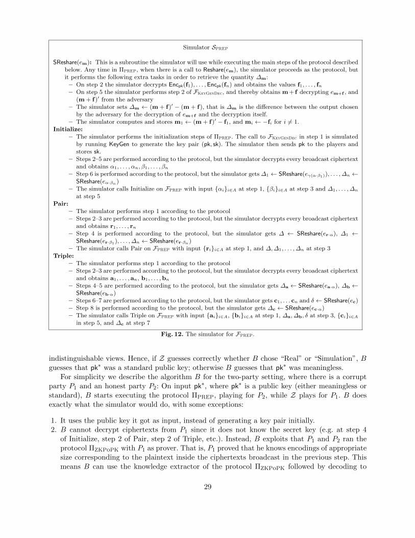
Simulator SPREP

SReshare(em): This is a subroutine the simulator will use while executing the main steps of the protocol describedbelow. Any time in ΠPREP, when there is a call to Reshare(em), the simulator proceeds as the protocol, butit performs the following extra tasks in order to retrieve the quantity ∆m:– On step 2 the simulator decrypts Encpk(f1), . . . ,Encpk(fn) and obtains the values f1, . . . , fn– On step 5 the simulator performs step 2 of FKeyGenDec, and thereby obtains m+ f decrypting em+f , and

(m + f)′ from the adversary– The simulator sets ∆m ← (m + f)′ − (m + f), that is ∆m is the difference between the output chosen

by the adversary for the decryption of em+f and the decryption itself.– The simulator computes and stores m1 ← (m + f)′ − f1, and mi ← −fi for i 6= 1.

Initialize:– The simulator performs the initialization steps of ΠPREP. The call to FKeyGenDec in step 1 is simulated

by running KeyGen to generate the key pair (pk, sk). The simulator then sends pk to the players andstores sk.

– Steps 2–5 are performed according to the protocol, but the simulator decrypts every broadcast ciphertextand obtains α1, . . . , αn, β1, . . . , βn

– Step 6 is performed according to the protocol, but the simulator gets ∆1 ← SReshare(eγ(α·β1)), . . . ,∆n ←SReshare(eα·βn)

– The simulator calls Initialize on FPREP with input αii∈A at step 1, βii∈A at step 3 and ∆1, . . . ,∆n

at step 5Pair:

– The simulator performs step 1 according to the protocol– Steps 2–3 are performed according to the protocol, but the simulator decrypts every broadcast ciphertext

and obtains r1, . . . , rn– Step 4 is performed according to the protocol, but the simulator gets ∆ ← SReshare(er·α), ∆1 ←

SReshare(er·β1), . . . ,∆n ← SReshare(er·βn)– The simulator calls Pair on FPREP with input rii∈A at step 1, and ∆,∆1, . . . ,∆n at step 3

Triple:– The simulator performs step 1 according to the protocol– Steps 2–3 are performed according to the protocol, but the simulator decrypts every broadcast ciphertext

and obtains a1, . . . ,an, b1, . . . ,bn– Steps 4–5 are performed according to the protocol, but the simulator gets ∆a ← SReshare(ea·α), ∆b ←

SReshare(eb·α)– Steps 6–7 are performed according to the protocol, but the simulator gets c1, . . . cn and δ ← SReshare(ec)– Step 8 is performed according to the protocol, but the simulator gets ∆c ← SReshare(ec·α)– The simulator calls Triple on FPREP with input aii∈A, bii∈A at step 1, ∆a,∆b, δ at step 3, cii∈A

in step 5, and ∆c at step 7

Fig. 12. The simulator for FPREP.

indistinguishable views. Hence, if Z guesses correctly whether B chose “Real” or “Simulation”, Bguesses that pk∗ was a standard public key; otherwise B guesses that pk∗ was meaningless.

For simplicity we describe the algorithm B for the two-party setting, where there is a corruptparty P1 and an honest party P2: On input pk∗, where pk∗ is a public key (either meaningless orstandard), B starts executing the protocol ΠPREP, playing for P2, while Z plays for P1. B doesexactly what the simulator would do, with some exceptions:

1. It uses the public key it got as input, instead of generating a key pair initially.2. B cannot decrypt ciphertexts from P1 since it does not know the secret key (e.g. at step 4

of Initialize, step 2 of Pair, step 2 of Triple, etc.). Instead, B exploits that P1 and P2 ran theprotocol ΠZKPoPK with P1 as prover. That is, P1 proved that he knows encodings of appropriatesize corresponding to the plaintext inside the ciphertexts broadcast in the previous step. Thismeans B can use the knowledge extractor of the protocol ΠZKPoPK followed by decoding to

29

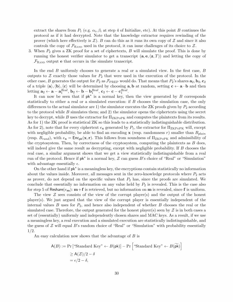
extract the shares from P1 (e.g. αi, βi at step 4 of Initialize, etc). At this point B continues theprotocol as if it had decrypted. Note that the knowledge extractor requires rewinding of theprover (which here effectively is Z). B can do this as it runs its own copy of Z and since it alsocontrols the copy of FRand used in the protocol, it can issue challenges of its choice to Z.

3. When P2 gives a ZK proof for a set of ciphertexts, B will simulate the proof. This is done byrunning the honest verifier simulator to get a transcript (a, e, (z, T )) and letting the copy ofFRand output e that occurs in the simulate transcript.

In the end B uniformly chooses to generate a real or a simulated view. In the first case, Boutputs to Z exactly those values for P2 that were used in the execution of the protocol. In theother case, B generates the output for P2 as FPREP would do. That means that P2’s shares a2,b2, c2of a triple 〈a〉, 〈b〉, 〈c〉 will be determined by choosing a,b at random, setting c ← a · b and thenletting a2 ← a− aReal1 , b2 ← b− bReal1 , c2 ← c− cReal1 .

It can now be seen that if pk∗ is a normal key, then the view generated by B correspondsstatistically to either a real or a simulated execution: if B chooses the simulation case, the onlydifferences to the actual simulator are 1) the simulator executes the ZK proofs given by P2 accordingto the protocol while B simulates them; and 2) the simulator opens the ciphertexts using the secretkey to decrypt, while B uses the extractor for ΠZKPoPK and computes the plaintexts from its results.As for 1) the ZK proof is statistical ZK so this leads to a statistically indistinguishable distribution.As for 2), note that for every ciphertext ex generated by P1, the extractor for ΠZKPoPK will, exceptwith negligible probability, be able to find an encoding x (resp. randomness r) smaller than Bplain(resp. Brand), with ex = Encpk(x, r). This follows from soundness of ΠZKPoPK and admissibility ofthe cryptosystem. Then, by correctness of the cryptosystem, computing the plaintexts as B does,will indeed give the same result as decrypting, except with negligible probability. If B chooses thereal case, a similar argument shows that we get a view statistically indistinguishable from a realrun of the protocol. Hence if pk∗ is a normal key, Z can guess B’s choice of “Real” or “Simulation”with advantage essentially ε.

On the other hand if pk∗ is a meaningless key, the encryptions contain statistically no informationabout the values inside. Moreover, all messages sent in the zero-knowledge protocols where P2 actsas prover, do not depend on the specific values that P2 has, since the proofs are simulated. Weconclude that essentially no information on any value held by P2 is revealed. This is the case alsofor step 5 of Reshare(em): m+f is retrieved, but no information on m is revealed, since f is uniform.

The view Z sees consists of the view of the corrupt player(s) and the output of the honestplayer(s). We just argued that the view of the corrupt player is essentially independent of theinternal values B uses for P2, and hence also independent of whether B chooses the real or thesimulated case. Therefore, the output generated for the honest player(s) seen by Z is in both cases aset of (essentially) uniformly and independently chosen shares and MAC keys. As a result, if we usea meaningless key, a real execution and a simulated execution are statistically indistinguishable, andthe guess of Z will equal B’s random choice of “Real” or “Simulation” with probability essentially1/2.

An easy calculation now shows that the advantage of B is

A(B) := Pr [“Standard Key”← B(pk)]− Pr[“Standard Key”← B(pk)

]≥ A(Z)/2− δ= ε/2− δ,

30

for some negligible δ that accounts for the differences between the involved distributions. However,if ε is non-negligible, then ε/2− δ is also non-negligible, which contradicts the assumption on thatmeaningless keys are statistically indistinguishable from standard ones. ut

A.6 Distributed Decryption

Proof (Theorem 4). The requirement B + 2sec · B < q/2 implies that t′ = t mod p, since ‖ri‖∞ <2sec ·B/(n · p) for i = 1, . . . , n. Therefore the protocol allows players to retrieve the correct messageif all the players are honest.

We now build a simulator SDDec to work on top of FKeyGenDec, such that the adversary cannotdistinguish whether it is playing with the decryption protocol and FKeyGen or the simulator andFKeyGenDec. We let A denote the set of players controlled by the adversary.

Simulator SDDec

Key Generation: This stage is needed to distribute shares of a secret key.– Upon “start”, the simulator sends “start” to FKeyGenDec and obtains pk. Moreover, the simulator obtains

(ski)i∈A from the adversary.– The simulator (internally) sets random (ski)i/∈A such that (ski)i=1,...,n is a full vector of shares of 0.– The simulator sends pk to A.

Public Decryption: This stage simulates a public decryption.– Upon “decrypt c,B”, the simulator sends “decrypt c” to FKeyGenDec and obtains m = Decsk(c).– It then computes the value vi for all players except for an honest player Pj .– It then samples rj uniformly with infinity norm bounded by 2sec ·B/(n · p) and computes

tj ← −∑i6=j

vi + p · rj + encode(m).

– For each other honest player Pi, it computes ti honestly (using c, ski).– The simulator broadcasts the values (ti)i/∈A,i6=j , tj and obtains (t∗i )i∈A from the adversary.

– It then sends m′ ← decode((

tj +∑i∈A t∗i +

∑i/∈A,i6=j ti

)mod p

)to FKeyGenDec so that the ideal func-

tionality sends “Result m′” to all the players.Private Decryption: This stage simulates a private decryption.

– Upon “decrypt c,B to Pj”, the simulator sends “decrypt c to Pj” to FKeyGenDec.– If Pj is corrupt, the simulator obtains c,m = Decsk(c) from FKeyGenDec and acts as in the simulated

public decryption.– If Pj is honest, the simulator receives c from FKeyGenDec, t∗i from each corrupt player Pi and ti from

each honest player.• The simulator samples rj uniformly with infinity norm bounded by 2sec ·B/(n · p).• It evaluates tj ← −

∑i6=j vi + p · rj .

• It computes ε←(tj +

∑i∈A t∗i +

∑i/∈A,i6=j ti

)mod p

• Finally it sends δ ← decode(ε) to FKeyGenDec in order to get Decsk(c) + δ to Pj .

Fig. 13. The simulator for ΠDDec.

In a simulated decryption the adversary receives pk and (ti)i/∈A,i 6=j , tj from SDDec. The distri-bution of pk is the same as in a real conversation, since it was sampled using the same algorithmas in a real conversation. The distribution of simulated ti, i 6= j is statistically close to the realone, since ti was computed correctly using shares of a possible secret key. We can therefore focuson the case where all the players but one are dishonest. We first analyse the simulation of public

31

decryption, introducing a hybrid machine, and prove its output is statistically indistinguishablefrom Pj ’s output (in the real protocol) and perfectly indistinguishable from Pj ’s simulated output.

Hybrid: On input (ski)i=1,...,n, c, reconstruct sk, compute Decsk(c), sample rj uniformly with in-finity norm bounded by 2sec ·B/(n · p) and output tj ← −

∑i 6=j vi + p · rj + encode(m).

Notice that tj = vj−t+encode(m)+p ·rj . Now, for a distribution X, define ϕ(X) := p ·X+vj .Notice that tj = ϕ(U), where U denotes the uniform distribution over vectors of integral entriesbounded with infinity norm 2sec · B/(n · p); moreover, since t − encode(m) is a multiple of p, onecan write tj = ϕ(U + (encode(m)− t)/p). Notice that ‖(encode(m)− t)/p‖∞ ≤ (B + p)/p, so thedistribution U + (encode(m)− t)/p is statistically close to U , since the probability of distinguishingU + (encode(m)− t)/p and U is bounded by the ratio

‖(encode(m)− t)/p‖∞2sec ·B/(n · p) + (B + p)/p

≤ (B + p)/p

2sec ·B/(n · p) + (B + p)/p= O(n · 2−sec),

which is negligible. Therefore tj is statistically close to tj .What is left to prove is that the simulation of private decryption to an honest player Pj is

statistically indistinguishable from the real protocol. In the real protocol Pj computes tj and

m′ ← decode

(∑i∈A

t∗i +∑i/∈A

ti

).

In that case the error m′ −m introduced by the adversary depends only on the value

ε′ :=

(∑i∈A

(t∗i − ti)

)mod p

computed using the actual secret key. In the simulation the error introduced by the adversary is

ε =

tj +∑i∈A

t∗i +∑

i/∈A,i 6=j

ti

mod p =

(∑i∈A

(t∗i − ti)

)mod p,

computed using secret shares of 0. Since the secret sharing scheme has privacy threshold n and thesums involve at most n− 1 shares, the quantities ε and ε′ are statistically indistinguishable. ut

B A lower Bound for the Preprocessing

In this section, we show that any preprocessing matching the properties we have, must output thesame amount of data as we do, up to a constant factor. We use the following theorem for 2-partycomputation from [28]. It talks about a setting where the parties A,B have access to a functionalitythat gives a random variable U to A and V to B with some guaranteed joint distribution PUV ofU, V . Given this, the parties compute securely a function f : X × Y 7→ Z, where A holds x ∈ X ,and B holds y ∈ Y. This function should have the property that there exists inputs y1, y2 such thatfor all x 6= x′, f(x, y1) 6= f(x′, y1); and for all x, x′, f(x, y2) = f(x′, y2). In other words, for someinputs B learns all of A’s input, but other inputs B learns nothing new.

32

Theorem 6. Let f : X ×Y 7→ Z be a function with inputs y1, y2 as above. If there exists a protocolthat computes f securely with access to PUV and with error probability ε in the semi-honest model,then

H(V ) ≥ I(U ;V ) ≥ log |X | − 7(ε log |X |+ h(ε))

We will also need the following technical lemma

Lemma 1. Let R be a random variable defined over the natural numbers. Then there exists aconstant C such that E(R) ≥ H(R)− 1− C.

Proof (Lemma 1). Let

I :=

i | i ≥ log

(1

Pr[R = i]

).

Under such a definition, one can write H(R) as

H(R) =∑i∈I

Pr[R = i] · log

(1

Pr[R = i]

)+∑i/∈I

Pr[R = i] · log

(1

Pr[R = i]

)By the construction of I, one can bound the first summand as follows∑

i∈IPr[R = i] · log

(1

Pr[R = i]

)≤∑i∈I

Pr[R = i] · i

≤∑i

Pr[R = i] · i

= E(R).

For the second summand one needs to work a bit more. Let q(i) := log(1/Pr[R = i]). Then∑i/∈I

Pr[R = i] · log

(1

Pr[R = i]

)=∑i/∈I

2−q(i) · q(i).

We now claim that2−q(i) · q(i) ≤ 2i · i, for all 0 6= i /∈ I.

This happens if and only if2−q(i) · 2log(q(i)) ≤ 2−i · 2log(i).

Taking the logarithm of such relation one gets −q(i) + log(q(i)) ≤ −i+ log(i), which is equivalentto q(i)− log(q(i)) ≥ i− log(i).Since q(i) = log(1/Pr[R = i]) ≥ i for all i /∈ I, and i ≥ 1, the latter relation is always satisfied.Therefore, one can bound the second summand by C +

∑i≥1 2−i · i, where C = 2−q(0) · q(0).

Moreover∑

i≥1 2−i · i converges to 1, so the second summand can be bound by 1 + C.Finally, one can reassemble all the reasoning into one and get∑

i∈IPr[R = i] · log

(1

Pr[R = i]

)+∑i/∈I

Pr[R = i] · log

(1

Pr[R = i]

)≤ E(R) + C + 1.

The last inequality implies that H(R) ≤ E(R) + 1 + C ut

33

With this result, we can prove the lower bound claimed earlier:

Proof (Theorem 2). Suppose we have an on-line protocol π that satisfies the assumptions in thetheorem. Consider any player Pi and suppose we want to compute the function

fT ((x,x′), y) = yx + (1− y)x′.

Here y ∈ Fpk and x,x′ are vectors over Fpk of length T . Pi will have input y and each Pj , j 6= i willhave as input substrings xj ,x

′j such that the concatenation of all xj (x′j) is x (x′). Finally, only

Pi learns the output fT ((x,x′), y).Clearly, fT can be computed using a circuit of size O(T ), and this will be the circuit promised

in the theorem. Note that our assumed protocol π can handle circuits of size S and can thereforecompute fT securely where T is Θ(S).

We can now transform π to a two-party protocol π′ for parties A and B. A has input x,x′, Bhas input y and B is supposed to learn fT ((x,x′), y). Now, π′ simply consists of running π where Bemulates Pi and A emulates all other players. We give to B whatever Pi gets from the preprocessingand A gets whatever the other players receive, so this defines the random variables U and V . Sinceπ is secure if Pi is corrupt and also if all other players are corrupt, this trivially means that π′ isan actively secure two-party protocol for computing fT .

This implies that π′ also computes fT with passive security. As noted in [28], this is actually notnecessarily the case for all functions. The problem is that if the adversary is passive, then activesecurity does guarantees that there is a simulator for this case, but such a simulator is allowed tochange the inputs of corrupted parties. A simulator for the passive case is not allowed to do this.However, [28] observe that for some functions, an active simulator cannot get away with changingthe inputs, as this would make it impossible to simulate correctly. They show this is the case forOblivious Transfer which is essentially what fT is after we go to the 2-party case. We may thereforeassume π′ is also passively secure.

Finally, we define f ′T (x, y) = fT ((x,0), y) = yx. Obviously π′ can be used to compute f ′Tsecurely, A just sets her second input to be 0. Moreover f ′T satisfies the conditions in Theorem6. So we get that H(V ) ≥ log |X | − 7(ε log |X | + h(ε)). If we adopt the standard convention thatthe security parameter grows linearly with the input size log |X | then because ε is negligible in thesecurity parameter, we have that the “error term” 7(ε log |X |+ h(ε)) is o(log |X |).

So we get that H(V ) is Ω(log |X |) = Ω(T log pk) = Ω(S log pk), since T is Θ(S). Recalling thatH(V ) is actually the entropy of the variable Pi received in the original protocol π, we get the firstconclusion of the Theorem.

For the second conclusion about the computational work done, it is tempting to simply claimthat B has to at least read the information he is given and so H(V ) is a lower bound on theexpected number of bit operations. But this is not enough. It is conceivable that in every particularexecution, B might only have to read a small part of the information.

It turns out that this does not happen, however, which can be argued as follows: let B(V ) bethe random variable representing the bits of V that B actually reads. By inspection of the proof ofTheorem 6, one sees that if we replace everywhere V by B(V ) the same proof still applies. So in fact,we have H(B(V )) ≥ log |X | − 7(ε log |X | + h(ε)). Now let R be the random variable representingthe number of bits B reads from V .

If we condition on R, then the entropy of B(V ) cannot drop by more than H(R), so we have

H(B(V )|R) ≥ H(B(V ))−H(R) ≥ log |X | − 7(ε log |X |+ h(ε))−H(R).

34

Moreover, we also have

H(B(V )|R) =∑r

Pr(R = r)H(B(V )|R = r) ≤∑r

Pr(R = r)r = E(R)

Putting these two inequalities together, we obtain that

E(R) +H(R) ≥ log |X | − 7(ε log |X |+ h(ε)).

Now, either E(R) ≥ (log |X | − 7(ε log |X |+ h(ε)))/2, or H(R) ≥ (log |X | − 7(ε log |X |+ h(ε)))/2. Inthe latter case we have from Lemma 1 that E(R) is much larger than H(R), so we can certainlyconclude that E(R) ≥ (log |X |−7(ε log |X |+h(ε)))/2 in any case. As above, the error term dependingon ε becomes negligible for increasing security parameter, so we get that E(R) is Ω(S log pk) asdesired. ut

C Canonical Embeddings of Cyclotomic Fields

Our concrete instantiation will use some basic results of Cyclotomic fields which we now recap on;these results are needed for the main result of this Appendix which is a proof of a “folklore” resultabout the relationship between norms in the canonical and polynomial embeddings of a cyclotomicfield. This result is used repeatedly in our main construction to produce estimates on the size ofparameters needed.

C.1 Cyclotomic Fields

We first recap on some basic facts about numbers fields, and their canonical embeddings. Focusingparticularly on the case of cyclotomic fields.

Number Fields An algebraic number (resp. algebraic integer) θ ∈ C is the root of a polynomial(resp. monic polynomial) with coefficients in Q (resp. Z). The minimal polynomial of θ is the uniquemonic irreducible f(x) ∈ Q[X] which has θ as a root.

A number field K = Q(θ) is the field obtained by adjoining powers of an algebraic number θ toQ. If θ has minimal polynomial f(x) of degree N , then K can be considered as a vector space overQ, of dimension N , with basis 1, θ, . . . , θN−1. Note that this “coefficient embedding” is relativeto the defining polynomial f(x) Equivalently we have K ∼= Q[X]/f(X), i.e. the field of rationalpolynomials with degree less than N , modulo the polynomial f(X). Without loss of generality wecan assume K, from now on, is defined by a monic irreducible integral polynomial of degree N .The ring of integers OK of K is defined to be the subring of K consisting of all elements whoseminimal polynomial has integer coefficients.

Canonical Embedding There are N field morphisms σi : K −→ C which fix every element of Q.Such a morphism is called a complex embedding and it takes θ to each distinct complex root off(X). The number field K is said to have signature (s1, s2) if the defining polynomial has s1 realroots and s2 complex conjugate pairs of roots; clearly N = s1 + 2 · s2. The roots are numbered inthe standard way so that σi(θ) ∈ R for 1 ≤ i ≤ s1 and σi+s1+s2(θ) = σi+s1(θ) for 1 ≤ i ≤ s2. Wedefine σ = (σ1, . . . , σN ), which defines the canonical embedding of K into Rs1 × C2·s2 , where thefield operations in K are mapped into componentwise addition and multiplication in Rs1 × C2·s2 .To ease notation we will often write α(i) = σi(α), for α ∈ K. We will let ‖α‖p for p ∈ [1, . . . ,∞]denote the p-norm of α in the coefficient embedding (i.e. the p-norm of the vector of coefficients)and let ‖σ(α)‖p denote norms in the canonical embedding.

35

Cyclotomic Fields We will mainly be concerned with cyclotomic number fields. The mth cyclotomicpolynomial is given by Φm(X), this is an irreducible polynomial of degree N = φ(m). The numberfield defined by Φm(X) is said to be a cyclotomic number field, and is defined by K = Q(ζm), whereζm is an mth root of unity, i.e. a root of Φm(X). The ring of integers of K is equal to Z[ζm]. Thenumber field K is Galois, and hence (importantly for us) the polynomial splits modulo p (for anyprime p not dividing m) into a produce of distinct irreducible polynomials all of the same degree.

The key fact is that if Φm(X) has degree d factors modulo the prime p then m divides pd−1. Tosee this notice that if Φm(X) factors into N/d factors each of degree d then the finite field Fpd must

contain the mth roots of unity and so m divides pd − 1. In the other direction, if d is the smallestinteger such that m divides pd− 1 then Φm(X) will have a degree d factor since the decompositiongroup of the prime p in the Galois group will have order d.

C.2 Relating Norms Between Canonical and Polynomial Embeddings

There is a distinct difference between the canonical and polynomial embeddings of a number field.In particular notice the following expansions upon multiplication, for x, y ∈ OK ,

‖x · y‖∞ ≤ δ∞ · ‖x‖∞ · ‖y‖∞.‖σ(x · y)‖p ≤ ‖σ(x)‖∞ · ‖σ(y)‖p.

where

δ∞ = sup

‖a(X) · b(X) (mod f(X))‖∞

‖a(X)‖∞ · ‖b(X)‖∞: a, b ∈ Z[X],deg(a),deg(b) < N

.

In this section we show that one can more tightly control the expansion factor of elements in thepolynomial representation; as long as they are drawn randomly with a discrete Gaussian distribu-tion. In particular we prove the following theorem; this result is well known to people working inideal lattice theory, but proofs have not yet appeared in any paper.

Theorem 7. Let K denote a cyclotomic number field then there is a constant Cm, depending onlyon m, such that for all α ∈ OK we have

– ‖σ(α)‖∞ ≤ ‖α‖1.

– ‖α‖∞ ≤ Cm · ‖σ(α)‖∞.

We recall some facts about various matrices associated with roots of unity, see [26] and the fullversion of [22]. First some notation; for any integer m ≥ 2: We set ζm = exp(2 ·π ·

√−1/m) to be a

root of unity for an integer m. As usual we let N = φ(m) and we define Z∗m = am,i : 0 ≤ i < Nto be a complete set of representatives for Z∗m with 1 ≤ am,i < m. We let A ⊗ B, for matrices Aand B, denote the Kronecker product. We let It denote the t× t identity matrix. All a× b matricesM in this section will have elements mi,j indexed by 0 ≤ i < a and 0 ≤ j < b; i.e. we index fromzero; this is to make some of the expressions easier to write down. The infinity norm for a matrixM = (mi,j) is defined by

‖M‖∞ := max

N−1∑j=0

|mi,j |

N−1

i=0

.

36

We define the N ×N CRT matrix as follows:

CRTm :=(ζam,i·jm

)0≤i,j<N

.

Then we define the constant Cm in the above theorem as Cm = ‖CRT−1m ‖∞. From which the proofnow immediately follows:

Proof (Theorem 7). For a cyclotomic field the canonical embedding is given by the map σ(α) =CRTm ·α, where α is the vector of the coefficient embedding of α, i.e. α considered as a polynomialin θ a root of F (X) = Φm(X) and CRTm is the matrix, defined earlier, i.e. it is equal to

CRTm =

1 θ(1) . . . θ(1)N−1

......

...

1 θ(N) . . . θ(N)N−1

.

For the first part of the theorem we note that, on writing α =∑N−1

i=0 xi · θi, we have

∣∣∣α(i)∣∣∣ =

∣∣∣∣∣∣N−1∑j=0

xj · θ(i)j∣∣∣∣∣∣ ≤

N−1∑j=0

|xj | · |θ(i)j | =N−1∑j=0

|xj | = ‖x‖1 = ‖α‖1.

For the second part we note that for all β ∈ OK ,

‖β‖∞ = ‖CRT−1m · σ(β)‖∞ ≤ ‖CRT−1m ‖∞ · ‖σ(β)‖∞

from which the result follows. utThe key question then is how large can Cm become. So we now turn to this problem; giving apartial answer.

The m×m DFT matrix is defined by:

DFTm :=(ζi·jm)0≤i,j<m .

Let m′ be a divisor of m then for i ∈ 0, . . . ,m− 1 we write i0 = i mod m′ and i1 = (i− i0)/m′.We then define the m×m “twiddle matrix” to be the diagonal matrix defined by

Tm,m′ := Diagζi0·i1m

i=0,...,m−1 .

Finally we define Lmm′ to be the permutation matrix which fixes the row with index m−1, but sendsall other rows i, for 0 ≤ i < m − 1, to row i ·m′ mod m − 1. Following [26] we use these matricesto decompose the matrix Dm into D′m and Dk, where m = m′ · k, via the following identity

DFTm = Lmm′ · (Ik ⊗ DFTm′) · Tm,m′ · (DFTk ⊗ Im′) , (3)

This is nothing but the general Cooley-Tukey decomposition of the DFT for composite m. Considerthe Vandermonde matrix

V (x1, . . . , xm) :=

1 x1 x21 . . . xm−11

1 x2 x22 . . . xm−12...

......

...1 xm x2m . . . xm−1m

.

It is clear that DFTm = V (1, ζm, ζ2m, . . . , ζ

m−1m ).

37

Lemma 2. We have, for any m,

DFT−1m =1

m· V (1, ζ−1m , ζ−2m , . . . , ζ1−mm )

Proof. Let δi,j be defined so that δi,j = 0 if i 6= j and equal to one otherwise. We have(V (1, ζm, ζ

2m, . . . , ζ

m−1m ) ·V (1, ζ−1m , ζ−2m , . . . , ζ1−mm )

)i,j

=∑

0≤k<mζi·kn · ζ−k·jm

=∑

0≤k<mζk·(i−j)m = m · δi,j .

ut

This leads to the following lemma which gives shows that the infinity norm of the inverse of theDFT matrix is always equal to one.

Lemma 3. For any m we have ‖DFT−1m ‖∞ = 1.

Proof. If ζm is an m-th root of unity, it is clear that ‖V (1, ζm, ζ2m, . . . , ζ

m−1m )‖∞ = m. In addition

we have ψm = 1/ζm is also an m-th root of unity, thus

‖DFT−1m ‖∞ =1

m· ‖V (1, ψm, ψ

2m, . . . , ψ

m−1m )‖∞ =

m

m= 1.

ut

Let m = pe11 · · · pesk we define r = p1 · · · ps, m1 = m/r; hence N = φ(m) = φ(r) ·m1. In [22] the

authors specialise the decomposition (3) (by selecting appropriate rows and columns) in the casem′ = m1 and k = r, to show that to show that, upto a permutation of the rows, the matrix CRTmis equal to (

Iφ(r) ⊗ DFTm1

)· T ∗m,m1

· (CRTr ⊗ Im1)

where Tm,m1∗ is another diagonal matrix consisting of roots of unity. We then have that

Lemma 4. For an integer m ≥ 2 such that m = pe11 · · · pekk we write r = p1 · · · pk, we then have

Cm ≤ Cr.

Proof. As above we write m1 = m/r. First note that ‖A ⊗ It‖∞ = ‖Is ⊗ A‖∞ = ‖A‖∞ for anymatrix A and any integers s and t. Then also note that since CRTm is given, upto a permutationof the rows, by the above decomposition, we have that CRT−1m is given up to a permutation of therows by the decomposition (

CRT−1r ⊗ Im1

)· T−1 ·

(Iφ(r) ⊗ DFT−1m1

).

So we have

‖CRT−1m ‖∞ = ‖(CRT−1r ⊗ Im1

)· T−1 ·

(Iφ(r) ⊗ DFT−1m1

)‖∞,

≤ ‖CRT−1r ⊗ Im1‖∞ · ‖T−1‖∞ · ‖Iφ(r) ⊗ DFT−1m1‖∞,

= ‖CRT−1r ‖∞ · ‖T−1‖∞ · ‖DFT−1m1‖∞ = ‖CRT−1r ‖∞.

ut

38

This result means that we can bound Cm for infinite families of values of m, by simply deducing abound on Cr, where r is the product of all primes dividing m. For example notice that CRTr = (1)and hence C2e = C2 = 1 for all values of e. Indeed it is relatively straight forward to determine theexact value of Cp for a prime p:

Lemma 5. If p is a prime then

Cp =2 · sin(π/p)

p · (cos(π/p)− 1).

Proof. 7 First note that it is a standard fact from algebra (by consider inverses of Vandermondematrices for example) that the entries of a row of the matrix CRT−1p are given by the coefficientsof the polynomial

Φp(X)

Φ′p(ζp) · (X − ζp), (4)

where each row uses a different root of unity ζp. We then note that

Φ′p(ζp) = (ζp − ζ2p ) · (ζp − ζ3p ) · · · (ζp − ζp−1p )

= ζ−2p · (1− ζp) · (1− ζ2p ) · · · (1− ζp−2p ) · (1− ζp−1p )

(1− 1/ζp)

=ζ−2p p

1− 1/ζp=

p

ζ2p − ζp.

Thus the coefficients of the polynomial in (4) are given by ζp · (ζrp −1)/p for r = 1, . . . , p−1. Whereeach row of our matrix is given by a different pth root ζp.

Thus to determine the infinity norm of CRT−1p we simply need to sum the absolute values ofthese coefficients, for the first row, since all other rows will be equal:

Cp =

p−1∑r=1

|ζp(ζrp − 1)/p| = 1

p

p−1∑r=1

√2− 2 · cos(2rπ/p)

=1

p

p−1∑r=1

2 · sin(rπ/p) =2 · sin(π/p)

p · (cos(π/p)− 1)

ut

In practice this result means that Cp ≈ 4/π ≈ 1.2732 for all p ≥ 11.If m is odd then we see that, subject to a permutation of the rows, the matrix CRT2m and

CRTm are identical up to a multiple of −1 for every second column. Thus we have

C2m = Cm for odd values of m.

We find that Cr ≤ 8.6 for squarefree r ≤ 400, which provides a relatively small upper bound onCm for an infinite family of cyclotomic fields K. It appears that the size of Cm depends crucially onthe number of prime factors of m. Thus it is an interesting open question to provide a tight upperbound on Cm. Indeed the growth in Cm seems to be closely related to the growth in the coefficientsof the polynomial Φm(X), which also depends on the number of prime factors of m.

7 This proof was provided to us by Robin Chapman .

39

C.3 Application of the above bounds

An immediate consequence of Theorem 7 is to provide an upper bound on the value δ∞ for cyclo-tomic number fields. Let α ∈ OK then we have, by the standard inequalities between norms, that‖α‖1 ≤ N · ‖α‖∞. Thus we have, for α, β ∈ OK ,

‖α · β‖∞ ≤ Cm · ‖σ(α · β)‖∞ ≤ Cm · ‖σ(α)‖∞ · ‖σ(β)‖∞≤ Cm · ‖α‖1 · ‖β‖1≤ Cm ·N2 · ‖α‖∞ · ‖β‖∞,

i.e. δ∞ ≤ Cm · N2. When m is a power of two, since Cm = 1 we find the bound δ∞ ≤ φ(m)2;however in this case it is known that δ∞ = φ(m), thus the above bound is not tight.

A more interesting application, for our purposes, is to bound the infinity norm in the polynomialembedding of the product of two elements which have been selected with a discrete Gaussian. Todemonstrate this result we will first need to introduce the following standard tailbound:

Lemma 6. Let c ≥ 1 and C = c · exp(1−c2

2 ) < 1 then for any integer N ≥ 1 and real r > 0 we have

Prx←DZN,s

[‖x‖2 ≥ c · s ·

√N

2 · π

]≤ CN .

Note that this implies that

Prx←DZN,s

[‖x‖2 ≥ 2 · r ·

√N]≤ 2−N ,

where r = s/√

2 · π. If we therefore select α, β ∈ DZN ,s, consider them as elements of OK , we then

have, with overwhelming probability that ‖α‖2, ‖β‖2 ≤ 2 · r ·√N . We then apply the standard

inequality between the 2- and the 1-norm to deduce ‖α‖1, ‖β‖1 ≤ 2 · r ·N . We then have that

‖α · β‖∞ ≤ Cm · ‖σ(α · β)‖∞ ≤ Cm · ‖σ(α)‖∞ · ‖σ(β)‖∞≤ Cm · ‖α‖1 · ‖β‖1≤ 4 · Cm · r2 ·N2.

D Security, Parameter Choice and Performance

In this Appendix we show that our concrete SHE scheme meets all the security requirementsrequired by our MPC protocol, i.e. that it is an admissible cryptosystem. On the way we deriveparameter settings, and finally we present some implementation results for the core operations.

Recall a cryptosystem is admissible if it meets the following requirements:

– It is IND-CPA secure.– It has a KeyGen∗ function with the required properties.– It is (Bplain, Brand, C)-correct, where Bplain = N · τ · sec2 · 2sec/2+8, Brand = d · ρ · sec2 · 2sec/2+8,

and where C, the set of functions we can evaluate on ciphertexts, contains all formulas evaluatedin the protocol ΠPREP’ (including the identity function). Note that here we choose the valuesfor Bplain, Brand that correspond to the most efficient variant of the ZK proofs.

Recall in the expressions for Bplain and Brand we have d is the dimension of the randomness space,i.e. d = 3 · N , τ is a bound on the infinity norm of valid plaintexts, i.e. p/2; and ρ is a bound onthe infinity norm of the randomness in validly generated ciphertexts, i.e. ρ ≈ 2 · r ·

√N , by the

tailbound of Lemma 6.

40

IND-CPA and KeyGen∗’s properties: We first turn to discussing security. Since our scheme isidentical (bar the distributed decryption functionality) to that of [7], security can be reduced tothe hardness of the following problem.

Definition 2 (PLWE Assumption). For all sec ∈ N, let f(X) = fsec(X) ∈ Z[X] be a polynomialof degree N = N(sec), let q = q(sec) ∈ Z be a prime integer, let R = Z[X]/f(X) and R = R/qR,and let χ denote a distribution over the ring R. The polynomial LWE assumption PLWEf,q,χ statesthat for any l = poly(sec) it holds that

(ai, ai · s+ ei)i∈[l] ≈ (ai, ui)i∈[l]

where s is sampled from the distribution χ, and ai, ui are uniformly random in Rq. We requirecomputational indistinguishability to hold given only l samples, for some l = poly(sec).

In particular our scheme is semantically secure if the PLWEΦm(X),q0,DNρ (s)-problem is hard. The

hardness of the same problem also implies that the output from KeyGen() is computationallyindistinguishable from that of KeyGen∗().

Thus our first task is to derive relationships between the parameters so as to ensure the firsttwo properties of being admissible are satisfied, i.e. the PLWE problem is actually hard to solve.The basic parameters of our scheme are the degree of the associated number field N = φ(m),the standard deviation r of the used Gaussian distribution, and the modulus q. We first turn toestimating r; we do this by using the “standard” analysis of the underlying LWE problem.

We first ensure that r is chosen to avoid combinatorial style attacks. Consider the underlyingLWE problem as being given by s ·A+ e = v, where e is the LWE error vector, and A is a randomN × t matrix over Fq. In [1] the authors present a combinatorial attack which breaks LWE in time

2O(‖e‖2∞) with high probability. Since e is chosen by the discrete Gaussian with standard deviationr, if we pick r large enough then this attack should be prevented. Thus choosing r such that r > 3.2will ensure that r is large enough to avoid combinatorial attacks, i.e. s ≥ 8.

We now turn to the distinguishing problem, namely given v can we determine whether it arisesfrom an LWE sample, or from a uniform sample. We determine a lower bound on N . The natural“attack” against the decision LWE problem is to first find a short vector w in the dual latticeΛq(A

T)∗ and then check whether w · vT is close to an integer. If it is then the input vector is anLWE sample, if not it is random. Thus to ensure security, following the argument in [23][Section5.4.1], we require

r ≥ 1.5

‖w‖2.

Following the work of [14] we can estimate, for t N , the size of the output of a lattice reductionalgorithm operating on the lattice Λq(A

T)∗. In particular if the algorithm tries to find a vectorwith root Hermite factor δ (thus δ measures the difficulty in breaking the underlying SHE system,typically one may select δ ≈ 1.005, but see later for other choices) then we expect to find a vectorw of size

1

qmin(q, δt · qN/t).

Following the analysis of [23] the above quantity is minimized when we select t = t′ :=√N log(q)/ log(δ).

This leads us to the deduce the lower bound

r ≥ 1.5 ·max(1 , δ−t′ · q1−N/t′).

41

Noise of a Clean Ciphertext: We now turn to determining the bound, in the infinity norm,of the value obtained in decrypting valid ciphertexts. Consider what happens when we decrypt aclean ciphertext, encrypted via (c0, c1) = Encpk(x, r), with r = (u,v,w). This looks like a PLWEsample (c1, c0) where the “noise” term, for a validly generated clean ciphertext, is given by

t = c0 − s · c1= x + p · (e · v + w + s · u)

By our estimates in Appendix C.3 we can bound the infinity norm of t by

‖t‖∞ ≤p

2+ p ·

(4 · Cm · r2 ·N2 + 2 ·

√N · r + 4 · Cm · r2 ·N2

)=: Y.

(Bplain, Brand, C)-correctness: Whilst IND-CPA is about security in relation to validly createdciphertexts, our distributed decryption functionality must be secure even when some ciphertextsare not completely valid. This was why we introduced the notion of (Bplain, Brand, C)-correctness.We need to pick Bplain and Brand so that Bplain ≥ N ·τ ·sec2 ·2sec/2+8 and Brand ≥ d·ρ·sec2 ·2sec/2+8.Since Bplain Brand we estimate the noise term associated to such a “clean” ciphertext will bebounded by Y ′ = (Brand/ρ)2 · Y = 9 ·N2 · sec4 ·2sec+16 · Y . In our MPC protocol we only need tobe able to evaluate functions of the form

(x1 + · · ·+ xn) · (y1 + · · ·+ yn) + (z1 + · · ·+ zn).

We can, via the results in Appendix C.3, crudely estimate the size of B, from Section 6, needed toensure valid decryption. Our crude (over-) estimate therefore comes out as

B ≤ δ∞ · (n · Y ′) · (n · Y ′) + (n · Y ′)≤ Cm ·N2 · n2 · Y ′2 + n · Y ′

≤ Cm ·N2 · n2 · c2sec · Y 2 + n · csec · Y =: Z

where csec = 9 ·N2 · sec4 · 2sec+8. We take Z as the bound, which we then need to scale by 1 + 2sec

to ensure we have sufficient space to enable the distributed decryption algorithm. Hence, the valueof q needs to be selected so that Z · (1 + 2sec) < q/2.

So in summary we need to choose parameters such that

q > 2 · Z · (1 + 2sec),

r > max

3.2, 1.5 · δ−t′ · q1−N/t′,

where sec is the statistical security parameter, δ is a measure of how hard it is to break theunderlying SHE scheme, and t′ =

√N log(q)/ log(δ). This leads to a degree of circularity in the

dependency of the parameters, but valid parameter sets can be found by a simple search technique.

42

Specific Parameter Sets: To determine parameters for fixed values of (Fpk)s and n we proceedas follows. There are two interesting cases; one where p is fixed (i.e. p = 2) and one where we onlycare that p is larger than some bound (i.e. p > 232, or p > 264). The latter case of p > 264 is moreinteresting as such size numbers can be utilized more readily in applications since we can simulateinteger arithmetic without overflow with such numbers. In addition using such a value of p meanswe do not need to repeat our ZKPoKs, or replicate the MACs so as to get a cheating probabilityof less than 2−40.

Our method in all cases is to first fix p, n, sec and δ, we then search using the above inequalitiesfor (rough) values of q and N which satisfy the inequalities above. We then search for exact valuesof p and N which satisfy our functional requirements on p (i.e. fixed or greater than some bound)plus N larger than the bound above, such that N is the degree of F (X) = Φm(X) and F (X) splitsinto at least s factors of degree divisible by k over Fp.

Given this precise value for N , we then return to the above inequalities to find exact values ofq and r. In all our examples below we pick n = 3, sec = 40, and δ = 1.0052.

Example 1. We first look at p > 232. Our first (approximate) search reveals we need N > 14300,q ≈ 2430 and r = 3.2 (assuming Cm ≤ 2). We then try to find an optimal value of N ; this is doneby taking increasing primes p > 232 and factoring p− 1. The factors of p− 1 correspond to valuesof m such that Φm(X) factors into φ(m) factors modulo p. So we want to find a p such that p− 1is divisible by an m, so that N = φ(m) > 14300. A quick search reveals candidates of

(p,N,m) = (232 + 32043, 14656, 14657).

Picking m in this way will maximise the value of s = n, and hence allow us to perform moreoperations in parallel. In addition since m is prime we know, by Lemma 5, that Cm ≈ 1.2732, thusjustifying our assumption in deriving the bounds of Cm ≤ 2.

Selecting m to be the prime 14657 in addition allows us to evaluate s = p−1 = 14656 runs of thetriple production algorithm in parallel. The message expansion factor, given we require N · log2(q)bits to represent N elements in Fp is given by

N · log2(q)

N · log2(p)=

log2(q)

log2(p)=

430

32≈ 13.437.

Example 2. Performing the same analysis for a p > 264, our first naive search of parameters revealwe need an n ≈ 16700 and q ≈ 2500. We then search for specific parameters and find p = 264 + 4867is pretty near to optimum, which results in a prime value of m of 16729. We find the expansionfactor is given by

log2(q)

log2(p)=

500

64≈ 7.81.

Example 3. We now look at the case p = 2 and k = 8, i.e. we are looking for parameters whichwould allow us to compute AES circuits in parallel; or more generally circuits over F28 . Our firstapproximate search reveals that we need N > 12300, q ≈ 2370 and r = 3.2. So we now need todetermine a value m such that

N = φ(m) > 12100 and 2d ≡ 1 (mod m) and d ≡ 0 (mod 8).

43

A quick search reveals candidates of

(m,N) = (17425, 12800)

since Φ17425(X) factors into s = 320 factors of degree d = 40 modulo 2. Thus using this value of mwe are able to work with s = 320 elements of F28 in parallel. The message expansion factor, givenwe require N · log2(q) bits to represent 320 elements in F28 is given by

N · log2(q)

8 · s=d · 370

8= 1850.0

For this value of m we find C17425 ≈ 9.414.

We present the following run-times we have achieved. We time the operations for encryptingand decrypting clean ciphertexts, the time to homomorphically compute (cxcy)cz, plus the timeto decrypt the said result. The times are given in seconds, and in brackets we present the amortizedtime per finite field element. All timings were performed on an Intel Core-2 6420 running at 2.13GHz.

Enc Dec (Clean) (cx cy) cz Decsk((cx cy) cz)Example Time (s) Time (s) Time (s) Time (s)

1 0.72 0.00005 0.35 0.00002 1.43 0.0001 0.72 0.000052 3.13 0.00019 1.54 0.00009 6.27 0.0004 3.15 0.000183 1.26 0.00394 0.60 0.00188 2.46 0.0077 1.23 0.00384

Estimating Equivalent Symmetric Security Level: The above examples were computed usingthe root Hermite factor of δ = 1.005. Mapping this “hardness” parameter for the underlying latticeproblem to a specific symmetric security level (i.e. 80-bit security, or 128-bit security) is a bit of a“black art” at present.

In [9] the authors derive an estimate for the block size needed to obtain a given root Hermitefactor, assuming an efficient BKZ lattice reduction algorithm is used. They then provide estimatesas to the run time needed for a specific enumeration using this block size. As an example of theiranalysis they estimate that a block size of 286 is needed to obtain a root Hermite factor of δ = 1.005.Then they estimate that the run time needed to perform the enumeration in a projected lattice ofsuch dimension (the key sub-procedure of the BKZ algorithm) takes time roughly between 280 and2175 operations. Thus a value of δ = 1.005 can be considered secure; however their estimates arenot precise enough to produce parameters associated with a given symmetric security level.

In [20] the authors take a different approach and simply extrapolate run times for the NTLimplementation of BKZ. By looking at various LWE instances, they derive the following equationlinking the expected run-time of a distinguishing attack and the root Hermite factor

log2 T =1.8

log2 δ− 110.

The problem with this approach is that NTL’s implementation of BKZ is very old, and hence isnot state-of-the-art; on the other hand we are able to derive a direct linkage between δ and log2 T .Using this equation we find the following equivalences:

44

log2 T 80 100 128 196 256δ 1.0066 1.0059 1.0052 1.0041 1.0034

Using these estimates for δ we re-run the above analysis to find approximate values for N andq in our three example applications; again assuming n = 3 and sec = 40.

Fp : p > 232 Fp : p > 264 F28

N > log2 q ≈ N > log2 q ≈ N > log2 q ≈δ = 1.0066 11300 430 12900 490 9500 360δ = 1.0059 12600 430 14700 500 10900 370δ = 1.0052 14300 430 16700 500 12300 370δ = 1.0041 18600 440 21100 500 15600 370δ = 1.0034 22400 440 25500 500 18800 370

As can be seen the security parameter has only marginal impact on log2 q, and results in adoubling of the size of N as we increase from a security level of 80 bits to 256 bits. As a comparisonif we, for security level 128 bits, i.e. δ = 1.0052, increase the value of sec from 40 to 80 we find thefollowing parameter sizes:

Fp : p > 232 Fp : p > 264 F28

N > log2 q ≈ N > log2 q ≈ N > log2 q ≈δ = 1.0052 18700 560 21000 630 16700 500

E Functionalities

Functionality FRand

Random Sample: When receiving (rand) from all parties, it samples a uniform r ← 0, 1u and outputs(rand , r) to all parties.

Random modulo p: When receiving (rand , p) from all parties, it samples a uniform value e← Fpk and outputs(rand , e) to all parties.

Fig. 14. The ideal functionality for coin-flipping.

Functionality FAMPC

Initialize: On input (init , pk) from all parties, the functionality activates and stores the modulus p.Input: On input (input , Pi, varid , x) from Pi and (input , Pi, varid , ?) from all other parties, with varid a fresh

identifier, the functionality stores (varid , x).Add: On command (add , varid1, varid2, varid3) from all parties (if varid1, varid2 are present in memory and

varid3 is not), the functionality retrieves (varid1, x), (varid2, y) and stores (varid3, x+ y mod p).Multiply: On input (multiply , varid1, varid2, varid3) from all parties (if varid1, varid2 are present in memory

and varid3 is not), the functionality retrieves (varid1, x), (varid2, y) and stores (varid3, x · y mod p).Output: On input (output , varid) from all honest parties (if varid is present in memory), the functionality

retrieves (varid , x) and outputs it to the environment. If the environment inputs OK then x is output to allplayers. Otherwise ⊥ is output to all players.

Fig. 15. The ideal functionality for arithmetic MPC.

45

Functionality FPREP

Usage: We first describe two macros, one to produce [[v]] representations and one to produce 〈v〉 representations.We denote by A the set of players controlled by the adversary.

Bracket(v1, . . . ,vn,∆1, . . . ,∆n, β1, . . . , βn), where v1, . . . ,vn,∆1, . . . ,∆n ∈ (Fpk )s, β1, . . . , βn ∈ Fpk1. Let v =

∑ni=1 vi

2. For i = 1, . . . , n(a) The functionality computes the MAC γ(v)i ← v · βi and sets γi ← γ(v)i +∆i

(b) For every corrupt player Pj , j ∈ A the environment specifies a share γji(c) The functionality sets each share γji , j /∈ A, uniformly such that

∑nj=1 γ

ji = γi

3. The functionality sends (vi, (βi, γi1, . . . , γ

in)) to each honest player Pi (dishonest players already have

the respective data).Angle(v1, . . . ,vn,∆, α), where v1, . . . ,vn,∆ ∈ (Fpk )s, α ∈ Fpk

1. Let v =∑ni=1 vi

2. The functionality computes the MAC γ(v)← α · v and sets γ ← γ(v) +∆3. For every corrupt player Pi, i ∈ A the environment specifies a share γi4. The functionality sets each share γi i /∈ A uniformly such that

∑ni=1 γi = γ

5. The functionality sends (0,vi, γi) to each honest player Pi (dishonest players already have the respectivedata).

Initialize: On input (init , p, k, s) from all players, the functionality stores the prime p and the integers k, s. Itthen waits for the environment to call either “stop” or “OK”. In the first case the functionality sends “fail”to all honest players and stops. In the second case it does the following:1. For each corrupt player Pi, i ∈ A, the environment specifies a share αi2. The functionality sets each share αi, i /∈ A uniformly3. For each corrupt player Pi, i ∈ A, the environment specifies a key βi4. The functionality sets each key βi i /∈ A uniformly5. The environment specifies ∆1, . . . ,∆n ∈ (Fpk )s

6. It runs the macro Bracket(Diag(α1), . . . ,Diag(αn),∆1, . . . ,∆n, β1, . . . , βn).Pair: On input (pair) from all players, the functionality waits for the environment to call either “stop” or “OK”.

In the first case the functionality sends “fail” to all honest players and stops. In the second case it does thefollowing:1. For each corrupt player Pi, i ∈ A, the environment specifies a share ri2. The functionality sets each share ri, i /∈ A uniformly3. The environment specifies ∆,∆1, . . . ,∆n ∈ (Fpk )s

4. It runs the macros Bracket(r1, . . . , rn,∆1, . . . ,∆n, β1, . . . , βn) and Angle(r1, . . . , rn,∆, α).Triple: On input (triple) from all players, the functionality waits for the environment to call either “stop” or

“OK”. In the first case the functionality sends “fail” to all honest players and stops. In the second case itdoes the following1. For each corrupt player Pi, i ∈ A, the environment specifies shares ai,bi2. The functionality sets each share ai,bi, i /∈ A uniformly. Let a :=

∑ni=1 ai, b :=

∑ni=1 bi

3. The environment specifies ∆a,∆b, δ ∈ (Fpk )s

4. It sets c← a · b + δ5. For each corrupt player Pi, i ∈ A, the environment specifies shares ci6. The functionality sets each share ci, i /∈ A uniformly with the constrain

∑ni=1 ci = c

7. The environment specifies ∆c ∈ (Fpk )s

8. It runs the macros Angle(a1, . . . ,an,∆a, α), Angle(b1, . . . ,bn,∆b, α), Angle(c1, . . . , cn,∆c, α).

Fig. 16. The ideal functionality for making the global key [[α]], pairs [[r]], 〈r〉 and triples 〈a〉, 〈b〉, 〈c〉

46