aquatic pesticide monitoring program nonchemical ... is the most thermodynamically stable and...
TRANSCRIPT

Aquatic Pesticide Monitoring Program
SFEI Contribution 390February 2005
San Francisco Estuary Institute
Aquatic Pesticide Monitoring Program Nonchemical Alternatives
Year 3 Final Report
Ben GreenfieldNicole David
Geoffrey S. SiemeringThomas P. McNabb
David F. SpencerGregory G. Ksander
M. J. DonovanP. S. Liow
W. K. ChanSeth B. Shonkoff
Stephen P. Andrews, Jr.Joy C. AndrewsMichael Rajan
Vanessa HowardMark Sytsma
Sam EarnshawLars W.J. Anderson


Aquatic Pesticide Monitoring Program
Nonchemical Alternatives Year 3 Final Report
Ben K. Greenfield1, Nicole David 1, Geoffrey S. Siemering 1,Thomas P. McNabb2, David F. Spencer3, Gregory G. Ksander 3
M. J. Donovan 3, P. S. Liow 3, W. K. Chan 3, Seth B. Shonkoff 1Stephen P. Andrews, Jr.4, Joy C. Andrews 5, Michael Rajan 5
Vanessa Howard6, Mark Sytsma 6, Sam Earnshaw7
and Lars W.J. Anderson3
SFEI Contribution 390, February 2005

This report should be cited as: Greenfield, Ben K., N. David, G. S. Siemering, T. P. McNabb, D. F. Spencer, G. G.
Ksander, M. J. Donovan, P. S. Liow, W. K. Chan, S. B. Shonkoff, S. P. Andrews, J. C. Andrews, M. Rajan, V. Howard, M. Sytsma, S. Earnshaw, and L.W.J. Anderson. 2005. Aquatic Pesticide Monitoring Program Nonchemical Alternatives Year 3 Final Report. APMP Technical Report: SFEI Contribution 390. San Francisco Estuary Institute, Oakland, CA.
1 San Francisco Estuary Institute, Oakland, CA 2 Clean Lakes, Inc., Martinez, CA 3 USDA Agricultural Research Station, Davis, CA 4 Environmental Sciences Teaching Program, UC Berkeley, Berkeley, CA 5 California State University, Hayward, CA 6 Portland State University, Portland, OR 7 Community Alliance with Family Farmers, Watsonville, CA

TABLE OF CONTENTS Chapter 1 Lake Sweeper Evaluation 1
1.1. Introduction 11.2. Materials and Methods 2
Site Description 2Lake Sweepers 3
1.3. Experiment Overview 4Water Chemistry 4Mesocosm 4Measurement of Fragment Density 5Plant Biomass and Nutrient Content 5
1.4. Control Costs 61.5. Results and Discussion 6
Water Chemistry 6Mesocosm 8Measurement of Fragment Density 9Plant Biomass and Nutrient Content 10
1.6. Control Costs 111.7. Conclusion 12
Chapter 2 Mechanical Shredding of Hyacinth: Costs, Operation and Permitting 151.1. Introduction 151.2. Sampling Site And Methods 161.3. Results and Discussion 17
Project set-up and operational constraints 17Permitting 20Control cost 20
Chapter 3 Mechanical Shredding of Hyacinth: Survival and Regrowth 251.1. Introduction 251.2. Materials and Methods 26
Fragment Characteristics 28Waterhyacinth Abundance: Lambert Slough 32
1.3. Results 33Fragment Characteristics 33Waterhyacinth Abundance: Lambert Slough 43
1.4. Discussion 571.5. Epilogue 63
Chapter 4 Mechanical Shredding of Hyacinth: Water Quality Impacts 691.1. Introduction 691.2. Methods 71
Study Site - The Sacramento-San Joaquin Rivers Delta 71Shredding Operation 72Chemistry Analysis 73

Statistical Analysis 75Estimated nutrient mass released by a Delta wide shredding operation 76
1.3. Results 78General site conditions 78Variation in individual water chemistry attributes 78Dissolved oxygen and turbidity trends 81Overall variation in chemistry with shredding 85Estimated nutrient mass released by a Delta wide shredding operation 86
1.4. Discussion 88
Chapter 5 Fragment Propagules of Spartina alterniflora 961.1. Introduction 961.2. Materials & Methods 98
Field Study of Rototilling Effects 98Greenhouse Study 98Propagule Dispersal Study 99
1.3. Results 100Field Study of Rototilling Effects 100Greenhouse Study 102Propagule Dispersal Study 103
1.4. Discussion 1041.5. Conclusions 106
Chapter 6 Creeping Wildrye Riparian Buffer Strips 1081.1. Introduction 1081.2. Site Selection and Evaluation 1081.3. Site Analysis 1091.4. Planning and Planting 1101.5. Conclusion 113
Chapter 7 SolarBee Evaluation: Abstract 114

Nonchemical Alternatives Year 3 Final Report
1
CHAPTER 1 EVALUATING IMPACTS OF LAKE SWEEPER PLANT CONTROL
Nicole David 1, Ben K. Greenfield 1 and Geoffrey S. Siemering 1
ABSTRACT
The Lake Sweeper is a mechanical control technique for removing nuisance aquatic vegetation in small areas around docks. Direct impacts of the Lake Sweeper on water quality and the potential for spread of viable plant fragments were evaluated in this study. Analyses of water nutrient concentrations (total and dissolved phosphorus, nitrate and nitrite, and organic carbon) and measurements of conventional water quality parameters, as well as fragment density were conducted over a 10-day treatment period. A mesocosm experiment and plant biomass and nutrient estimations were also performed. The Lake Sweeper successfully removed all plant biomass without affecting nutrient concentrations or water quality in the treatment areas. The likelihood of spreading plant fragments is high, but in areas of extensive infestation, like the San Joaquin River Delta, this may not be a management concern. In general, the Lake Sweeper proved to be a successful, cost-effective, low maintenance plant control method for small areas where additional plant fragmentation is tolerable.
Key Words: mechanical control, fragments, re-growth, San Joaquin River, Egeria densa, Ceratophyllum demersum
1.1. INTRODUCTION
Introduced aquatic plants impair the use of water resources in many ways. Problems associated with exotic plants include degradation of water quality, interference with flood control measures, obstruction of boat traffic, and decreased recreational opportunities (Madsen 1997, 2004; Pimentel et al. 2000). The Lake Sweeper was invented as a non-chemical control method for small areas (up to 230 m2 at a time), particularly around docks, in water bodies that are infested with invasive plant species. Rooted plants are removed from the sediment and captured by underwater rakes that are pulled by a water pump driven floating arm. The floating arm cycles back and forth in an arc from a fixed attachment point. Arm length and cycling frequency can be modified as can rake depth. This study evaluates whether the Lake Sweeper can effectively eliminate nuisance plants from the treatment area and the potential impacts of this method on the nearby ecosystem. The Lake Sweeper has been well publicized (Kretsch 2003) but not yet independently studied. Potential impacts of this mechanical control method include water quality changes and production of viable fragments.
The Sacramento-San Joaquin River Delta (California, USA) is impacted by
introduced plant species, including Egeria densa (Brazilian Egeria) and Eichhornia crassipes (water hyacinth) (Bock 1969; Anderson 1990; California Department of Boating and Waterways 2001). Control of these plants using pesticide applications entails
Nonchemical Alternatives Year 3 Final Report
2
potential risks to both humans and wildlife. Due to the Talent decision (243 f. 3d 526 (9th Cir. 2001) Headwaters, Inc. vs. Talent Irrigation District, the U.S. Court of Appeals for the Ninth Circuit), National Pollution Discharge Elimination System (NPDES) permits and requisite monitoring are now required in California for application of aquatic herbicides. The permitting and monitoring costs have added considerable expense to chemical pesticide control options (Siemering 2004). Not only is the examination of alternative control methods required in NPDES permits, but the study of such methods may identify techniques that small businesses, including marinas, resorts, and other shoreline property owners may find useful, where the high regulatory costs of chemical pesticide applications make them prohibitive.
The Aquatic Pesticide Monitoring Program, funded by the California State Water
Resources Control Board, evaluated many non-chemical alternative control methods (Greenfield et al. 2004). One major concern with mechanical plant control methods is the spread of plant infestations due to an increased production of plant fragments. For species like Egeria, Ceratophyllum demersum (coontail), and Hydrilla verticillata, which reproduce by stem fragments (DiTomaso and Healy 2003), the production of viable fragments can cause re-infestation of a treated area or spread infestations to new regions. Long-term water quality impacts from re-suspension of particle-bound nutrients and other contaminants that were immobilized in the sediment are another concern, particularly for treatments which disturb sediments (Getsinger et al. 2002).
We performed an experimental application of the Lake Sweeper at three marina docks
to evaluate its cost effectiveness and environmental impacts. Paired treatment and reference stations were monitored for effects on water chemistry. The treated areas were sampled before and during treatment to assess the extent of fragment production, and a mesocosm study was set up to evaluate whether fragments in the treatment areas were viable. Finally, information was compiled to evaluate cost effectiveness of the Lake Sweeper.
1.2. MATERIALS AND METHODS
SITE DESCRIPTION Three marinas in the San Joaquin River Delta were chosen as study sites (Paradise
Point Marina, King Island Resort, and Ladd’s Stockton Marina) (Figure 1). They were all located on either the San Joaquin River or Disappointment Slough, within a six-mile radius of one another (within latitude N 37°58.616’ and N 38°03.394’ and longitude W 120°25.077’ and W 121°27.518’). At each marina, one treated site and one reference (untreated) site was established. The distance between treated and reference sites was 100 – 300 m. The sites were near frequently used boat slips and docks. The selected marinas had dense vegetation (more than 50% of the area covered by submerged plants). Egeria and coontail were the most abundant plant species at the study sites and therefore used in the mesocosm experiments. Both reproduce vegetatively by turions and stem fragments. Egeria produces neither fruits nor seeds in the western United States, whereas coontail also reproduces by seed (DiTomaso and Healy 2003). Additionally, Lemna minuscule

Nonchemical Alternatives Year 3 Final Report
3
(duckweed), Cabomba caroliniana (fanwort), Chladophera spp, Myriophyllum hippuroides (western water milfoil), Hydrocotyle ranunculoides (floating pennywort), and water hyacinth were present in minor amounts.
The study sites were subject to tidal cycles but salinity remained below two parts per
thousand. A week with moderate tides was selected for evaluation of treatment effectiveness and ecosystem impacts. Prior to treatment, carbon, nitrogen, and phosphorus concentrations in the water column were determined at all marinas. No significant differences between the treatment and reference sites were observed for these nutrients (Analysis of Variance p > 0.05 in all cases). All treatment and sampling events took place in July and August of 2004.
Figure 1. Study area in the Sacramento-San Joaquin River Delta.
LAKE SWEEPERS Two 36-foot and one 20-foot long Lake Sweeper units (Lake Restoration Inc.,
Rogers, MN) were deployed, one per marina. The Lake Sweepers operated 24 hours a day for ten consecutive days. Areas of 50 m2 at Ladd’s Stockton Marina, 130 m2 at King Island Resort, and 200 m2 at Paradise Point Marina were treated. The machines use a standard 110 V power outlet and draw 12.5 amperes. The life expectancy of the machines is estimated to be 10 years by the manufacturer, with a shorter life-time in salt and

Nonchemical Alternatives Year 3 Final Report
4
brackish water. A P 4400 Kill A WattTM Power Meter (P3 International Corporation, New York, NY) was used to determine the electricity consumed over the study period. The consumption per kilowatt-hour was determined to evaluate the cost of operating a Lake Sweeper. The hourly rate was calculated for Stockton, CA, where Pacific Gas & Electric charges $0.11 per kilowatt-hour.
1.3. EXPERIMENT OVERVIEW
WATER CHEMISTRY Water chemistry samples were taken prior to the start of the treatment period, as well
as 24, 72, and 240 hours into the treatment at the six different sites (three treated and three reference sites). Water quality parameters analyzed included total suspended solids (TSS), dissolved organic carbon (DOC), total organic carbon (TOC), as well as total phosphorus and dissolved ortho-phosphate. Ortho-phosphate is the most thermodynamically stable and biochemically available form of phosphorus in natural waters (Snoeyink and Jenkins 1980). Nitrate (NO3), nitrite (NO2), and total Kjeldahl nitrogen (TKN) were also analyzed. Total nitrogen was calculated as the sum of NO2,NO3 and TKN. These parameters were analyzed by the California Department of Fish and Game (Water Pollution Control Laboratory, Rancho Cordova, CA) and California Laboratory Services (Rancho Cordova, CA). Water samples were taken inside the treatment area at the midpoint boom rake radius, between sweeping cycles of the Lake Sweeper at 1 m water depth. Dissolved oxygen (DO), temperature, pH, electrical conductivity (EC), and turbidity were measured immediately below the water surface and at 1m depth at all stations using a WTW Multi 340i multimeter.
Statistical analyses of the Lake Sweeper treatment and reference plots were
performed using repeated measures Analysis of Variance (ANOVA). Repeated measures ANOVA is an appropriate method for modeling changes in environmental variables measured repeatedly over time in the same experimental sites (Von Ende 2001). Repeated measures ANOVA was performed on each chemical parameter, with evaluation of overall changes over four measurement dates, in addition to the impact of the Lake Sweeper treatment on nutrient levels over time (i.e., a date by treatment interaction). All measurements were assessed for statistical significance by comparing the Huynh-Feldt Epsilon corrected p-value to an α value of 0.05 (Von Ende 2001). All statistical analyses were performed in SAS (SAS Institute 1990).
MESOCOSM Mesocosm experiments were conducted to investigate the potential for plant fragment
re-growth. The fragment re-growth was evaluated on Egeria and coontail at the Paradise Point Marina. For each plant species, five gallon buckets were filled with 10 cm of relatively undisturbed sediment from the Paradise Point Marina reference site. Ten fragments of various lengths, generated by the Lake Sweeper, were planted into each of the first five buckets. Fragment size and number of nodes were recorded to document physical characteristics and determine the potential for re-growth (Sabol 1987). Five buckets were planted with ten intact plants from the reference site to function as a

Nonchemical Alternatives Year 3 Final Report
5
positive control in regards to overall growth conditions in the mesocosms. The remaining five buckets contained sediment only and no fragments, providing a negative control to show whether small fragments or coontail seeds were introduced into the mesocosm with the sediment. All buckets were closed with insect screen and rubber cords to avoid loss or mixing of fragments. The buckets were then secured with rebar at the bottom of a shallower part of the marina (about one meter depth at low tide) where the mesocosms were covered by water at all times. Four to five times during the test period, the insect screens were cleaned with a soft brush to maintain sufficient light exposure and water exchange for the plants. Repeated measures ANOVA was used to document significant changes in growth characteristics for the positive control and experimental plant samples over time (Von Ende 2001).
MEASUREMENT OF FRAGMENT DENSITY Plant fragment samples were collected before the Lake Sweeper operation, three
through six days into the operation, and ten days after the start. Within the treated area, a three-gallon bucket sieve (0.5 mm diameter) with a floatation device was dragged for 10 m through the water with the mouth of the bucket perpendicular to the water surface. This method was repeated five times at random locations throughout the treatment area. Fragments were keyed, counted, and measured for wet weight, number and length of stems, and number of nodes. To determine differences in fragment characteristics, changes were assessed over three measurement dates at the three different marinas using repeated measures ANOVA (Von Ende 2001).
PLANT BIOMASS AND NUTRIENT CONTENT To evaluate the effectiveness of the Lake Sweeper, three grabs of plant samples were
taken at each marina with a metal rake from the bottom of random areas inside the treatment zone. The rake samples were conducted at the beginning, the middle and the end of the study period. The plant material, collected by the rake with one swoop, was brought to the surface, spun in a salad spinner, and weighed to evaluate the efficacy and progress of the sweeping operation (Treibitz et al. 1993). Since the size of the area sampled with each grab may have varied, the results were only used to estimate relative changes in plant abundance over the course of the experiment.
Furthermore, 0.5 cubic meter of an untreated, shallower area was marked for plant
density samples. A volume rather than an area was chosen for this experiment to capture floating as well as rooted plants. The plants in this volume were removed, keyed, counted, measured, and weighed.
Characteristics determined included weight (wet weight per 500 liter), number of stem fragments per 500 liter, number of stem fragments per unit wet weight (stem density), and nodal distribution (number of nodes per stem).
To determine plant nutrient concentration estimates, eight plant samples were taken at
the Paradise Point Marina and King Island Resort. Four samples were taken from the reference sites and four from within the treatment area at the beginning of the sweeping operation. Four of the plant samples (two each from the reference and treated areas) were collected in shallower areas (< 1 m depth) and four from deeper areas (about 2 m depth).

Nonchemical Alternatives Year 3 Final Report
6
After being dried for 48 hours at 80°C and ground to fine powder, the plants were analyzed for total nitrogen and total carbon using a Perkin-Elmer Model 2400 CHN analyzer with acetanilide as a standard (Eadie 1997). Tissue phosphorus was determined on dried ground samples using the method described by Anderson and Ingram (1993).
1.4. CONTROL COSTS
Information on purchase prices (http://www.lakerestoration.com), labor for installation and maintenance (personal communication with Kevin Kretsch, Lake Restoration, Inc.), and fees for electricity (personal communication with PG & E Stockton, CA) were compiled to evaluate the control costs of the Lake Sweeper. Chemical application cost included NPDES permit fees (U.S EPA, 1999), costs for herbicides and labor (personal communication with Jay Kasheta, licensed applicator for Cygnet Enterprises West, Inc.), and costs for monitoring and reporting (based on an average of analytical costs for northern California laboratories) were calculated for comparison purposes.
1.5. RESULTS AND DISCUSSION
WATER CHEMISTRY Repeated measures ANOVA provided no evidence that the Lake Sweeper operation
influenced site water chemistry during the treatment period. Chemical parameters evaluated for statistical significance included dissolved oxygen, electrical conductivity, total organic carbon, total suspended solids, turbidity, total nitrogen, total phosphorus, and ortho-phosphate (Table 1).
No significant difference between the three Lake Sweeper treated and the reference stations was found for any of these chemical parameters during the treatment period (p > 0.05 in all cases). Dissolved organic carbon concentrations were predominantly non-detects. Graphical analysis indicated close correspondence between treatment and reference samples from each location, with no apparent difference resulting from the Lake Sweeper treatment (e.g., Figure 2).
The study results suggest that sweeping of selected areas is unlikely to have significant impacts on water quality. Few changes in water chemistry were observed at the experimental and reference sites, with slight fluctuations probably due to tidal cycles, since the variations at the treated and reference sites were consistent. The majority of samples were taken during slack tide after high tide but the exact sampling time relative to tidal cycles varied slightly among samples. The absence of strong patterns may be related to the small scale of this operation in comparison to larger scale mechanical harvesting projects (e.g., Carpenter and Adams 1976, 1978; Carpenter and Gasith 1978; Alam et al. 1996).

Nonchemical Alternatives Year 3 Final Report
7
Table 1. Mean results and standard error for water chemistry parameters for all three treatment and reference (Ref) sites. Samples were averaged for 1 m and surface readings for conventional water quality parameters.
Event DO EC pH TOCTotal
Phosphorus
Dissolved ortho-
Phosphate
Dissolved Nitrate +
Nitrite TKN TSSmg/L µS mg/L mg/L mg/L mg/L mg/L mg/L
Pre 4.96±0.40 327±91 7.5±0.06 1.8±0.14 0.08±0.01 0.08±0.01 0.58±0.23 0.47±0.05 3.7±0.54
24 hrs 5.38±0.61 326±86 7.6±0.02 2.53±0.58 0.1±0.02 0.08±0.02 0.67±0.29 0.5±0.09 4.03±0.25
72 hrs 5.14±0.55 320±87 7.6±0.04 2.83±0.25 0.09±0.02 0.07±0.01 0.52±0.22 0.59±0.12 3.87±0.07
10 days 6.84±0.11 327±84 7.9±0.09 2.53±0.45 0.09±0.02 0.08±0.01 0.41±0.17 0.51±0.11 4.57±0.44
Pre-Ref 4.72±0.86 322±159 7.6±0.1 1.65±0.45 0.09±0.02 0.07±0.02 0.57±0.39 0.44±0.07 4.07±0.73
24 hrs-Ref 5.41±1.3 319±152 7.7±0.2 3.35±1.19 0.1±0.04 0.08±0.03 0.69±0.52 0.45±0.17 5.5±1.59
72 hrs-Ref 5.71±0.92 319±154 7.6±0.04 2.67±0.9 0.09±0.03 0.07±0.02 0.58±0.43 0.51±0.15 4.5±0.9
10 days-Ref 5.58±1.88 315±147 7.7±0.1 3.13±1.54 0.09±0.03 0.08±0.03 0.52±0.39 0.66±0.27 4.0±0.47
Sampling Events
pre 24 hrs 72 hrs 10 days
0
1
2
3
4
5
6
7
Paradise PointKings IslandLadd's Stockton
Figure 2. Total organic carbon concentrations at all study sites. Note that broken lines indicate treated site concentrations, solid lines indicate reference sites.

Nonchemical Alternatives Year 3 Final Report
8
MESOCOSM A decline in the total number of plant fragments was recorded for the positive control
and the experimental mesocosms for Egeria and for the experimental buckets for coontail using repeated measures ANOVA. Two to seven fragments per bucket disintegrated for coontail and two to ten fragments per bucket for Egeria (Table 2). The remaining experimental coontail fragments showed a slight increase in maximum length (7.6 cm) and maximum number of nodes (6 nodes) over the three-week test period (Table 2). However, no significant difference was displayed in comparison to the control regarding maximum length (p = 0.77; N = 10) and nodal distribution (p = 0.17; N = 10). For Egeria, repeated measures ANOVA suggested that the maximum number of nodes among remaining fragments of the experimental buckets increased significantly (p = 0.002; N = 10) compared to the positive control (Table 2). All negative controls showed no growth.
The observed increase in growth for coontail and Egeria fragments was expected
because these plant species spread through fragmentation (DiTomaso and Healy 2003). Since these fragments were collected in close vicinity of the Lake Sweeper during treatment, the results suggest that the Lake Sweeper operation does result in viable fragment production. Decreasing fragment numbers for the positive control of Egeria were probably caused by high amounts of particulate matter being moved around during each tidal cycle. The insect screens covering the buckets closest to the dock rapidly overgrew with algae and filled up with silt. Even brushing the screens several times during the test period probably did not allow for sufficient light to the buckets at all times. Although DiTomaso and Healy (2003) stated that Egeria grows best under low light (± 100 lux) and that coontail tolerates low light levels, disintegration of plant fragments and occasional loss of leaves suggested that light may have been a limiting factor for the growth experiment. Table 2. Averaged mesocosm results and standard deviations for coontail and Egeria densa.
Treatment Measurement Type Start End Start End
Experiment Max Length 35.2 ± 10.2 42.8 ± 19.6 34.2 ± 12.4 29.4 ± 13.1
Positive Control Max Length 49.8 ± 21.5 46 ± 16.3 32.6 ± 11.6 10 ± 16.5
Experiment Max Nodes 16.4 ± 4.7 22.4 ± 8.3 31.8 ± 13.6 48.6 ± 23.4
Positive Control Max Nodes 20.6 ± 4.5 22 ± 5.3 39.2 ± 9.7 7.8 ± 12.3
Experiment Number of Fragments 10 ± 0 6.6 ± 2.6 10 ± 0 8.4 ± 2.1
Positive Control Number of Fragments 10 ± 0 10.6 ± 1.3 10 ± 0 0.8 ± 1.3
Coontail Egeria

Nonchemical Alternatives Year 3 Final Report
9
MEASUREMENT OF FRAGMENT DENSITY Repeated measures Analysis of Variance did provide evidence that Lake Sweeper
treatment influenced Egeria and coontail fragment production over time. A significant change was found in both the abundance (Huynh-Feldt Epsilon corrected p = 0.048; N = 3) and total mass (Huynh-Feldt Epsilon corrected p = 0.030; N = 3) of fragments collected over three sampling dates at the three treatment sites. Figure 3 indicates a substantial increase in fragment abundance and mass three to six days after Lake Sweeper installation, with a decline to original abundance and mass eight to ten days after installation. Repeated measures ANOVA did not provide evidence of changes in Egeria fragment average stem length or number of nodes, or in any coontail fragment attributes (p > 0.05; N = 3 in all cases) over the three sampling events.
Fragments of Egeria and coontail in all size classes were present in the samples taken within the treatment area. Fragments accumulated in bundles mostly around the dock where the Lake Sweeper swept them. Often fragments stuck to the rakes and were pulled along with the movement of the arm. The experiment indicated a similar increase in Egeria and coontail fragment mass and stem number after three days at all three marinas. Fragment mass was about 50 times higher at days three to six of the treatment period than it was before the start. The number of stems was approximately 35 times higher during the same time period. At day ten, fragment mass and stem numbers per sample were almost back to the initial occurrence at all three experimental sites.
The results of the fragment tests suggest that over a short time period (two to nine
days) fragmentation of plants in the treated area will increase drastically, although plant fragments will be present at all times. In addition to the Lake Sweeper generated fragments, fragments can be generated naturally, by boat traffic, or by other mechanical control operations, and these fragments, regardless of source, can potentially cause reintroduction of new plants (Olem and Flock 1990). The manufacturer of the Lake Sweeper recommends an operation time of initially seven days to clear submerged aquatic weeds from an area. According to our results, after that time period, the generated fragments floating in the water seemed to have dispersed and only a slightly higher number of fragments remain in the treatment area after ten days (Figure 3).

Nonchemical Alternatives Year 3 Final Report
10
Sampling Events
1st Day 3rd - 6th Day 10th Day1
10
100
1000
Total Mass in gramsNumber of Fragments
Figure 3. Measurement of fragment weight and stem density during the study period. Note log scale on y-axis.
PLANT BIOMASS AND NUTRIENT CONTENT In general, nuisance plant control was achieved in the treatment areas within ten days.
For Paradise Point Marina and King Island Resort, rake plant biomass went almost down to zero at the end of the 10-day study period (Figure 4). In between day one and day six an average of 397 g of plant material was brought up with a single rake sample (range of 78 g to 1546 g). At day 10, treatment areas at both marinas showed almost no plants at the bottom. At Ladd’s Stockton Marina, the weight of scooped up samples was evenly distributed over the sampling period with an average of 356 g for the nine samples taken (average on day 1 = 359 g, on day 5 = 313 g, and on day 10 = 397 g). At this marina, the plant material was initially very thick, and the rakes of the machine had to be positioned closer to the surface in order for the machine to function. Progress was made by lowering the rakes over time, but the clean-up of this area was not accomplished within the period of this study.
Plant tissue nitrogen (N) concentrations showed high variation in the King Island
Resort samples. The overall mean tissue N differed among sites and depths (1 to 2 m), with an overall coefficient of variation of 42%. The shallow part of the reference site had the lowest mean value of 2.9%. The overall N:P ratios varied from 9.7 to 34.0 and were generally higher at King Island Resort compared to Paradise Point Marina, though there was no significant difference between the two sites (two-tail t-test: p = 0.08). The average N:P ratio for aquatic plants and algae is similar to that of terrestrial plants and lies at

Nonchemical Alternatives Year 3 Final Report
11
about 12 to 13 (Guesewell and Koerselman 2002; Knecht and Goeransson 2004). The high N:P ratio and lower P concentration seen at the deeper part of the King Island Resort, suggest a stronger phosphorus limitation (Cornett 2001).
Sampling Events
1st Day 3rd-6th Day 10th Day0
200
400
600
800
1000
1200
PP KI LS
Figure 4. Mean rake samples and standard error taken over the 10-day study period. PP = Paradise Point Marina, KI = King Island Resort, LS = Ladd’s Stockton Marina.
Mean tissue C varied from 22.0 to 31.3% with a C:N ratio between 4.0 and 8.6.
Relatively lower carbon concentrations (22 to 23% at Paradise Point Marina and 26 to 27% at King Island Resort) were observed for the reference sites of this study. Carbon concentrations in Egeria and coontail plant tissue were relatively low for summer sampling as compared to the 35 to 40% mean tissue concentrations determined by Spencer and Ksander (1999a). This resulted in lower C:N ratios than usual; seasonal and spatial variability are common in tissue nutrient concentrations (e.g., Spencer and Ksander 1999b).
1.6. CONTROL COSTS
In comparison to chemical treatment, the Lake Sweeper appeared to be a low cost method for small areas. It controlled plant growth in the treatment plots for about half the estimated cost of an application of Komeen (chelated copper) or Reward (diquat dibromide) in a similar size area. The initial purchase cost for each Lake Sweeper was approximately $2,000, installation and maintenance (two visits) were $600, and the

Nonchemical Alternatives Year 3 Final Report
12
electricity costs for the machine was estimated at $0.07 per hour, ($24 for the two-week treatment period). The cost for each Lake Sweeper operation thus totaled approximately $2,624. The Lake Sweeper could also be repositioned within a marina to broaden the treatment area. For comparison, the current California aquatic pesticide NPDES permit fee is $1,000, event-based monitoring, laboratory analysis, and reporting by a scientific consulting firm was estimated at $4,000, and the cost for chemicals and labor was $174, for a total cost of approximately $5,174 (for an area of approximately 200 m2). Both treatment types most likely would have to be repeated during the growing season, with additional chemical and monitoring costs for the pesticide treatment. In addition, amortization of the Lake Sweeper purchase costs over its ten year life span would result in considerably lower per anum costs when compared to chemical weed control.
1.7. CONCLUSION
The Lake Sweeper achieved the removal of nuisance aquatic plants from the marina near dock areas in a short time frame and appears to be a viable option for similar small areas needing control. Although the clean up was effective in the treated area, the fact that reproduction and dispersal of these plants via fragments of shoots and rhizomes (rooted or free floating) occurs indicates the need to consider additional factors when evaluating the effectiveness of the Lake Sweeper method (Parsons 1997; Anderson 2000; Greenfield et al. 2004). In the Stockton area, an increased fragment production of Egeria and coontail may not impose a higher risk for spreading the plant infestation, since these species are already widely distributed and cover about 3,900 acres in the Sacramento-San Joaquin Delta (Pennington 2004). In areas where there is little additional infestation, the increased fragment production by the Lake Sweeper could have significant consequences. Impacts on water quality due to the operation were not significant. An earlier treatment start date (e.g., in April or May) could have minimized maintenance effort and shortened treatment time due to less plant growth and less density in plant mats in spring and the beginning of the summer. In comparison to chemical treatments, the Lake Sweeper costs significantly less for treating very small areas of plant infestations.
ACKNOWLEDGEMENTS
We thank Kevin Kretsch with Lake Restoration Inc. and Jay Kasheta with Cygnet Enterprises West, Inc. for their cooperation effort and help with the purchase and installation of the Lake Sweepers. We thank Brian Healy and the Paradise Point Marina staff, as well as Bud Camper from King Island Resort, and Patty Bonnifield and the Ladd’s Stockton Marina for giving us access to the sampling sites and for contributing their time and support. William Haller, University of Florida, and David Spencer, UC Davis, provided valuable support with project planning and design. David Spencer and Greg Ksander, UC Davis, also performed plant nutrient concentration analysis. We thank Dave Crane and Martice Vasquez with the California Department of Fish and Game, Fish and Wildlife Water Pollution Control Laboratory and Ray Oslowski with California Laboratory Services for sample analyses. Thanks to Lester McKee and John Ross from the San Francisco Estuary Institute for helpful feedback and comments. Also thanks to

Nonchemical Alternatives Year 3 Final Report
13
Jennifer Hayworth and Chuck Striplen for planning and logistical support as well as field assistance during the entire project. This project was funded by the California State Water Resources Control Board, agreement # 01-130-250-2.
REFERENCES
Alam, S.K., L.A. Ager, T.M. Rosegger. 1996. The Effects of Mechanical Harvesting of Plant Tussock Communities on Water Quality in Lake Istokpoga, Florida. Journal of Lake and Reservoir Management, Vol. 12, No. 4, pp. 455-461.
Anderson, L.W.J. 1990. Aquatic Weed Problems and Management in Western United States and Canada. In: A.J. Pieterse, K.J. Murphy (eds.): Aquatic Weeds: The Ecology and Management of Nuisance Aquatic Vegetation. Oxford University Press, Oxford, England, pp. 371-391.
Anderson, J.M. and J.S.I. Ingram. 1993. Tropical Soil Biology and Fertility: A Handbook of
Methods (2nd edition) EAB International, Wallingford, United Kingdom, pp. 221.
Anderson, L.W.J. 2000. Dissipation of Sonar and Komeen following typical applications for control of Egeria densa in the Sacramento/San Joaquin Delta, and production and viability of E. densa fragments following mechanical harvesting. In: Egeria densa control program – Vol. II: Research Trial Reports, California Department Boating and Waterways, 15, pp. 2000.
Bock, J.H. 1969. Productivity of Water Hyacinth Eichhornia crassipes (Mart.) Solms. Ecology, Vol. 50 (3), pp.460-464.
California Department of Boating and Waterways. 2001. Environmental Impact Report for the Egeria densa Control Program. Sacramento, California, Vol. 4.
Carpenter, S.R. and M.S. Adams. 1976. The Macrophyte Tissue Nutrient Pool Of A Hardwater Eutrophic Lake: Implications for Macrophyte Harvesting. Aquatic Botany, Vol. 3, pp. 239-255.
Carpenter, S.R. and M.S. Adams. 1978. Macrophyte Control by Harvesting and Herbicides: Implications for Phosphorus Cycling In Lake Wingra, Wisconsin. Journal of Aquatic Plant Management, Vol. 16, pp. 20-23.
Carpenter, S.R. and A. Gasith. 1978. Mechanical Cutting of Submerged Macrophytes: Immediate Effects on Littoral Water Chemistry and Metabolism. Water Research, Vol. 12, pp. 55-57.
Cornett, V.C. 2001. Spatial Characterization of the Distribution of Submerged Aquatic Vegetation in the Shark River Slough Estuary. Department of Biology Sciences, Florida International University.
DiTomaso, J.M. and E.A. Healy. 2003. Aquatic and Riparian Weeds of the West. Regents of the University of California, Division of Agriculture and Natural Resources, Publication 3421.
Eadie, B.J. 1997. Standard Operating Procedure for Perkin Elmer Analyzer CHN (Model 2400). NOAA/Great Lakes Environmental Research Lab, Ann Arbor, MI 48105-1593.
Getsinger, K.D., A.G. Poovey, W.F. James, R.M. Stewart, M.J. Grodowitz, M.J. Maceina, and R.M Newman. 2002. Management of Eurasian Watermilfoil in Houghton Lake, Michigan: Workshop Summary. US Army Corps of Engineers. Aquatic Plant Control Research Program, ERDC/EL TR-02-24.
Greenfield, B.K., N. David, J.A.Hunt, M.Wittmann, G.S. Siemering. 2004. Aquatic Pesticide Monitoring Program. Review of Alternative Aquatic Pest Control Methods for California Waters. 2004. San Francisco Estuary Institute, Oakland, CA. http://www.sfei.org/apmp/apmpindex.html
Guesewell S. and W. Koerselman. 2002. Variation in Nitrogen and Phosphorus Concentrations of Wetland Plants. Perspectives in Ecology, Evolution and Systematics, Vol. 5, pp. 37 61.
Knecht, M.F. and A. Goeransson. 2004. Terrestrial Plants Require Nutrients in Similar Proportions. Tree Physiology, Vol. 24, pp. 447-460.
Kretsch, K. 2003. An Automated Aquatic Weed Control System for Shoreline Property Owners. 22nd Annual Western Aquatic Plant Management Society Meeting, Sacramento, California.
Madsen, J.D. 1997. Methods for Management of Non-indigenous Aquatic Plants. In: J.O.

Nonchemical Alternatives Year 3 Final Report
14
Luken, J.W. Thieret (eds.): Assessment and Management of Plant Invasions. Springer, New York, pp. 145-171.
Madsen, J.D. 2004. Invasive Aquatic Plants: A Threat to Mississippi Water Resources. Mississippi State University, Mississippi State, MS 39762-9652.
Olem, H. and G. Flock, eds. 1990. Lake and Reservoir Restoration Guidance Manual. 2nd edition. EPA 440/4-90-006. Prepared by North American Lake Management Society for US Environmental Protection Agency.
Parsons, J. 1997. Egeria densa – An Emerging Problem in the Western United States. Abstracts for The Western Aquatic Plant Management Society, May 1997. Washington Department of Ecology, Olympia, WA.
Pennington, T. 2004. Egeria densa Project. Portland State University, Center for Lakes and Reservoirs. Portland, Oregon 97207-0751.
Pimentel, D., L. Lach, R. Zungia, D. Morrison. 2000. Environmental and Economic Cost of Non-indigenous Species in the United States. BioScience, Vol. 50 (1), pp.53-68.
Sabol, B.M. 1987. Environmental Effects of Aquatic Disposal of Chopped Hydrilla. Journal of Aquatic Plant Management, Vol. 25, pp. 19-23.
SAS Institute. 1990. SAS/STAT User's Guide, Version 6, Fourth Edition. Cary, NC, SAS Institute.
Siemering, G. 2004. Aquatic Pesticide Monitoring Project Report Phase 2 (2003)
Monitoring Project Report. SFEI Contribution 108. San Francisco Estuary Institute, Oakland, CA.
Snoeyink, V.L., and D. Jenkins, 1980, Water Chemistry: New York, John Wiley & Sons.
Spencer, D.F. and G.G. Ksander. 1999a. Phenolic Acids and Nutrient Content for Aquatic Macrophytes from Fall River, California. Journal of Freshwater Ecology, Vol. 14, pp. 197-209.
Spencer, D.F. and G.G. Ksander. 1999b. Seasonal Changes in Chemical Compostion of Eurasian Watermilfoil (Myriophyllum spicatum L.) and Water Temperature at two Sites in Northern California: Implications for Herbivory. Journal of Aquatic Plant Management, Vol. 37, pp. 61-66.
Trebitz, A.S., S.A. Nichols, S.R. Carpenter, R.C. Lathrop. 1993. Patterns of vegetation change in Lake Wingra following a Myriophyllum spicatum decline. Aquatic Botany, Vol. 46, pp. 325-340.
U.S. EPA. 1999. The United States Experience with Economic Incentives for Protecting the Environment. EPA Report Number: EE-0216B, Chapter 4.
Von Ende, C.N. 2001. Repeated-measures analysis: growth and other time dependent measures. Design and Analysis of Ecological Experiments. S.M. Scheiner and J. Gurevitch. New York, Oxford University Press, pp. 134-157.
FOOTNOTES
1Corresponding author San Francisco Estuary Institute 7770 Pardee Lane Oakland, CA 94621 [email protected]

Nonchemical Alternatives Year 3 Final Report
15
CHAPTER 2 CONTROL COSTS, OPERATION, AND PERMITTING ISSUES FOR
MECHANICAL SHREDDING OF WATER HYACINTH: A CASE STUDY ON THE SACRAMENTO-SAN JOAQUIN RIVERS DELTA, CALIFORNIA
Ben K. Greenfield 1 and Thomas P. McNabb 2
ABSTRACT
Given the recent requirement for NPDES permitting to apply aquatic pesticides in the western United States, nonchemical aquatic plant control methods are receiving renewed attention. This study evaluates mechanical shredding as a potential alternative method for controlling water hyacinth (Eichhornia crassipes (Mart.) Solms) in the Sacramento-San Joaquin Delta, California. In fall 2003 and spring 2004, three mechanical shredding boats were operated on two representative Delta sites, to evaluate permitting issues, operational constraints, and control cost. Two boats (the AquaPlant Terminator and the Cookie Cutter) were operable in all conditions, provided there was sufficient water depth (> 0.3-0.6 m ). A third boat (the Amphibious Terminator) was difficult to maneuver, could not chop large plants, and repeatedly got mired in dense vegetation. Control cost varied widely as a function of plant size. In the fall, control costs in three of four sites were greater than $1600/acre. In the spring, control cost ranged from $200 to $900/acre, comparable to chemical pesticide application.
Key words: mechanical control, cost-effectiveness, restoration, Eichhornia crassipes
1.1. INTRODUCTION
Control cost effectiveness frequently influences the method selected for aquatic plant control. Two factors that determine cost-effectiveness are the area of infestation controlled per unit effort and the frequency the control method must be implemented. For mechanical cutting, the area controlled per unit effort is influenced by plant density, site access, obstructions, and the type of cutting machine employed. The rate of plant regrowth and recruitment varies widely among individual plant species depending on cutting location on the plant, cutting frequency, season, and other factors (Kimbel and Carpenter 1981; Cooke et al. 1990; Methé et al. 1993; Crowell et al. 1994; Unmuth et al. 1998; Fox et al. 2002). In recent years, peer reviewed studies on cost of mechanical plant control have been rare, despite the development of modified control equipment, and geographic information systems to accurately measure area controlled. In most management scenarios, due to concerns about spreading the infestation or influx of nutrients into the pelagic zone, cut plants are harvested and removed from the water body. This substantially increases control cost when compared to leaving cut vegetation in the water.
In the Sacramento-San Joaquin Rivers Delta, in northern California (hereafter, the
Delta), substantial infestations of water hyacinth (Eichhornia crassipes) have been routinely controlled for decades, using chemical herbicide applications, introduction of insects for biocontrol, and limited mechanical control trials (Anderson 1990). Given the

Nonchemical Alternatives Year 3 Final Report
16
regulatory burden of NPDES permitting, in addition to pressure from local advocacy groups, new alternative methods are being evaluated. The California Department of Boating and Waterways (CDBW) is conducting mechanical harvesting and manual removal on a limited basis, but disposal time, labor costs, and landfill costs are significant (California Department of Boating and Waterways 2001). Some local stakeholders have pushed for evaluation of mechanical shredding of aquatic vegetation, allowing the vegetation to remain in the water, as a less cost-prohibitive alternative to vegetation harvesting.
The purpose of this study was to evaluate the operational, permitting, and cost issues
associated with treating representative water hyacinth infestations from the Delta, using mechanical shredding. The paper discusses three issues: 1) set up and technical feasibility of the method, including operational limitations on when it would work; 2) permitting issues, with the focus on endangered species permitting; and 3) control cost. This paper expands upon a previously published extended abstract (Greenfield 2004), providing new unpublished data on control cost, treatment area, technical feasibility, and permitting issues. Control effectiveness, i.e., the ability of the method to kill the plants and inhibit future growth, is thoroughly evaluated in a separate paper (Spencer et al. 2005).
1.2. SAMPLING SITE AND METHODS
Two Delta sites were chosen for shredding evaluation, the Stone Lakes National Wildlife Refuge (Elk Grove, California; Latitude Longitude) and Dow Wetlands (Antioch, California; latitude longitude). The Dow Wetlands site is strongly tidally influenced, difficult to access, and densely infested with water hyacinth. The Stone Lakes Site has limited tidal flux and contains long narrow irrigation ditches. The Dow site is more characteristic of the conditions that the California Department of Boating and Waterways must contend with in controlling hyacinth. Stone Lakes is more representative of waterways that local landowners (irrigated agriculture and vineyards) must manage.
For the fall 2003 evaluation, a contract was established with Master’s Dredging, a
contractor that designs, builds and operates a mechanical shredder specialized for control of dense floating macrophyte infestations. This contractor was selected based on review of studies on the contractor’s prior performance (e.g., Stewart and McFarland 2000; James et al. 2002) and checking references with agency personnel having prior experience with the contractor. The contractor has two types of shredders. The “AquaPlant Terminator” is a boat that is 28 ft. long and 8 ½ ft. wide. Weighing 6 tons, it is equipped with sets of shredding blades at the front and rear of the boat, and separate engines to operate each set of blades (Figure 1). The “Amphibious Terminator” is a modified barge, having a standard airboat fan to propel the vessel, and a set of flail chopper blades at the front of the vessel (Figure 2).
For the spring 2004 evaluation, the “Cookie Cutter,” a commercially available
shredding vessel, was studied. A local contractor (Clean Lakes, Inc.) leased the vessel and operated it on-site. The Cookie Cutter has cutting blades that rotate in a direction

Nonchemical Alternatives Year 3 Final Report
17
perpendicular to the long axis of the boat (Figure 3). It is primarily used for cutting channels through dense emergent vegetation and shallow sediments. It has been marketed for water hyacinth control in Lake Victoria, Africa, but scientific studies of its effectiveness are lacking. Photographs of the cutting blades of all three vessels are available in an unpublished report (Spencer et al. 2005).
Control cost was evaluated at several locations varying in access difficulty and plant
size. This project calculated control cost as shredding area per dollar spent. Shredding area was determined using georectified aerial photographs of the site within one week of shredding or direct GPS field measurements of the shredding area on site (Figure 4). Dollars spent equaled the number of hours required to shred that location multiplied by the contractor's billing rate for the operation. Heights of uncut plants were determined at East Lambert Slough (October 6, 2003; mean = 22 cm; N = 10), and at the Dow Wetlands in the Fall (September 26, 2003; mean = 87 cm; N = 20) and Spring (June 6, 2004; mean = 18; N = 20 plants). Heights of uncut plants at West Lambert Slough ranged widely (range = 50 to 90 cm), with increased plant heights at the western end of the slough. Plant heights were not determined at the South Stone Lake site. At each site, plant density was estimated as one of three categories: loose, dense, or very dense.
1.3. RESULTS AND DISCUSSION
PROJECT SET-UP AND OPERATIONAL CONSTRAINTS In general, the AquaPlant Terminator and Cookie Cutter were both able to maneuver
in Delta hyacinth stands. Boat ramps used to launch the shredders required a packed gravel or concrete surface and sufficient draft in the vicinity (approximately 5 feet of depth). Otherwise, cranes were needed. The AquaPlant Terminator required 2 m water depth to launch and 1 m depth to operate effectively. With hyacinth plants taller then 0.6 m, the Terminator could only operate the rear set of shredding blades; operation of the front flail chopper blades brought shredded plant material directly onto the bow of the vessel. The Cookie Cutter also required about 1 m of water depth in the rear of the vehicle, but was capable of cutting channels in soft sentiment with the cutting blades.
The airboat shredder only required about 0.2 m of draft to operate. However, this
experimental vessel had many operational difficulties, severely limiting its utility for hyacinth control in the Delta. The airboat shredder was unsuccessful at shredding hyacinth greater than 0.5 m in stalk length (a size frequently encountered in the Delta between August and October; Spencer and Ksander 2005), and actually got mired in the vegetation on two separate occasions. The airboat also could not handle the strong winds or wave conditions characteristic of open waters of the central Delta. Finally, the airboats had a very wide turning radius and could not operate in reverse, significantly limiting the circumstances in which operation could occur. At one Stone Lake site, an irrigation ditch about 15 m wide, the operators had to turn the vessel around manually.

Nonchemical Alternatives Year 3 Final Report
18
Figure 1. The AquaPlant Terminator, with a view of the rear cutting blades, engine, and cut plant material. Note that there is another set of cutting blades on the front end of the vehicle, which is similar in design to the Cookie Cutter (not shown). Photo credit: Bob Case, Contra Costa County Department of Agriculture.
Figure 2. The Amphibian Terminator. Note the cut plant material in the foreground, uncut plant material in the background, and airboat fan on the rear of the vehicle.

Nonchemical Alternatives Year 3 Final Report
19
Figure 3. The Cookie Cutter. Photo credit: Krist Jensen, Dow Wetlands.
Figure 4. Arial view of Dow Wetlands, with GIS shape files of the five areas shredded by the Cookie Cutter in 2004 (Table 1).

Nonchemical Alternatives Year 3 Final Report
20
PERMITTING Permitting required for widespread application of mechanical shredding in California
waters would include the Federal Endangered Species Act Biological Opinion process to evaluate impacts on endangered and threatened species. The NEPA/CEQA process to evaluate discharge of pollutants into the water body might also be required, depending on the inclinations of the local permitting agency representative. For the present project, the NEPA/CEQA permitting was simplified, after personnel from the Central Valley Regional Water Quality Control Board indicated that the proposed research operation would not require formal application, provided that impacts were clearly documented and provided to the regulatory agencies. Other permitting issues (e.g. Army Corps of Engineers streambed alteration permits) were not addressed in this pilot-scale project, but would need to be addressed for a Delta scale operation.
Endangered species permitting presents a significant challenge for any large-scale
management action in the Delta, as the listed sensitive species include giant garter snake, Winter run Chinook salmon, the Delta smelt, and Valley elderberry longhorn beetle. In May 2003, a consultation was initiated with USFWS and NMFS to evaluate impact on endangered species. Within several months of initial contact, both agencies provided official letters indicating that formal consultation was not required, and permitting the project provided that: 1) efforts be made to minimize impacts on listed species; and 2) the project occur within the dates when sensitive species are least likely to be adversely affected (between July 15 and October 31). With approval given, a fall evaluation was conducted in late September, 2003.
A second evaluation was planned for the later spring/ early summer of 2004, when it
was expected that the plants would be smaller and more susceptible to shredding (Madsen et al. 1993). This evaluation occurred during the active movement and spawning stages of Chinook salmon, Delta smelt, and giant garter snake. To address these issues, a formal consultation was initiated with NOAA Fisheries and USFWS in November 2003. The USFWS consultation was completed by January, 2004. However, by May, 2004, the NOAA formal consultation was still not completed. At that time, the NOAA agency representative determined that listed fish species had already passed through the area for spawning, and provided a letter allowing the project to proceed without a formal consultation. Although NPDES permitting was not required for mechanical shredding at an experimental scale, large-scale operations would require extensive lead times (> 6 to 12 months) for endangered species permitting.
CONTROL COST Control costs ranged widely, depending on the density and plant size of the stand
(Table 1). In Fall of 2003, shredding efficiency was lowest at the Dow Wetland, where dense plant stands averaging 87 cm tall severely impeded shredding rate. At this site, it took 2 full days to shred 0.9 acre, resulting in a control cost greater than $7000/acre (Table 1) (Greenfield 2004). With such large and dense plants, only the rear set of Terminator chopping blades could be operated, and plants needed to be approached from an oblique angle to achieve any cutting. The plants were so densely packed that after an

Nonchemical Alternatives Year 3 Final Report
21
Table 1. Description of shredding plots, including site conditions, shredding area, time, and control cost. ND = not determined.
Site (Stations) Treatment Treatment Dates Site Conditions Shredded Area(acres)
Time(hr) Acres/hr $/Acre
East LambertSlough
AmphibiousTerminator 9/6, 9/8/2003 Dense a; 22 cm stem
height 3.5 3 1.18 $338 b
West LambertSlough
AquaPlantTerminator
9/19 - 9/21, 9/26 -9/27/2003
Dense; 45 – 90 cmstem height 11.7 49.5 0.24 $1,686
bSouth StoneLake
AmphibiousTerminator 9/28 - 9/29/2003 ND 1.8 7.5 0.25 $1,625
bDow Wetlands(DD)
AquaPlantTerminator 9/21 - 9/24/2003 Very Dense; 87 cm
stem height 0.9 17 0.05 $7,441b
Dow Wetlands(DD) Cookie Cutter 6/3/2004 Loose; 18 cm stem
height 1.3 2 0.63 $349
Dow Wetlands(DC) Cookie Cutter 6/3/2004 Loose; 18 cm stem
height 0.3 0.5 0.56 $393
Dow Wetlands(DB) Cookie Cutter 6/3/2004 Loose; 18 cm stem
height 1.1 1 1.14 $193
Dow Wetlands(DA) Cookie Cutter 6/3/2004 Loose; 18 cm stem
height 0.6 2.25 0.27 $825
Dow Wetlands(DE) Cookie Cutter 6/3/2004 Loose; 18 cm stem
height 0.2 0.75 0.25 $868
98 plants/m2 measured at East Lambert SloughPreviously published in Greenfield (2004)

Nonchemical Alternatives Year 3 Final Report
22
area was initially shredded, new uncut materials were observed to press back into that area from an adjacent unshredded location. Shredding costs were also high at West Lambert Slough and South Stone Lake, approximately $1700/acre in both cases (Table 1). Costs were relatively low in the East Lambert Slough site, with the Amphibious Terminator able to rapidly proceed through the 22 cm tall hyacinth. Overall, the rate of shredding of the large hyacinth was extremely slow, compared to evaluation of the AquaPlant Terminator on water-chestnut. In that study, the Boat was able to shred approximately three acres of water chestnut per hour (Stewart and McFarland 2000).
In the spring of 2004, control costs using the Cookie Cutter were much lower. At the
five separate Dow Wetland shredding sites in 2004, shredding cost (not including transport fees) ranged from $200 to $900 per acre (Table 1). The much lower control cost probably resulted from the relatively small plant size and low plant density. The spring shredding costs were relatively low, compared to the costs of chemical treatment methods presently employed. For comparison, the current California aquatic pesticide NPDES permit fee is $1,000, event-based monitoring, laboratory analysis, and reporting by a scientific consulting firm was estimated at $4,000, and the cost for chemicals and labor was $174, for a total cost of approximately $5,174 (for an area of approximately 200 m2).
For large infestations of water hyacinth, targeted herbicide application is considered
substantially more cost-effective than mechanical harvesting (Thomas and Anderson 1984; Cofrancesco 1996; Haller 1996). The present study indicates that costs of mechanical shredding without harvesting may be comparable to chemical treatment. In that western United States, recent legal developments are causing increases in regulatory costs and risks associated with chemical pesticide use. Following an Acrolein spill in an Oregon irrigation district, the U.S. Ninth Circuit Court of Appeals determined that aquatic pesticides discharged into any system that drains into U.S. natural waterways must be considered pollutants under the Clean Water Act (U.S. Ninth Circuit Court of Appeals 2001). As a result of this decision, all applicators within the Ninth Circuit Court jurisdiction (California, Oregon and Washington) are now required to obtain NPDES permits prior to applying aquatic pesticides. The regulatory paperwork and monitoring costs for this NPDES permitting can be considerable, and California agencies that have not strictly adhered to this process have faced costly litigation.
A number of management concerns impede widespread use of shredding as an
alternative to chemical pesticide application or more costly mechanical harvesting. These include transfer of nutrients to the water column (James et al. 2002), and release of heavy metals such as mercury (Riddle et al. 2002). But the primary risk associated with shredding water hyacinth is that the shredding operation itself may result in increased spread and recruitment of plants, ultimately worsening the infestation. In fact, in all of the shredding operations we evaluated, hyacinth fragments viable for regrowth were produced (Spencer et al. 2005). Therefore, mechanical shredding without harvesting would only be appropriate in the following circumstances: 1. extremely dense infestations, where boat access must be obtained quickly due to safety or economic

Nonchemical Alternatives Year 3 Final Report
23
considerations; 2. isolated waterways already infested in all available littoral habitat; or 3. if it can be demonstrated experimentally that the shredding operation does not produce more viable fragments than would be generated by the natural recruitment of the plant. Because the Delta consists of multiple connected waterways, with considerable interannual variation in hyacinth density, large-scale shredding operations should not be conducted there until effective mortality can be demonstrated.
ACKNOWLEDGEMENTS
The following people provided invaluable assistance with planning and field operations for this study: Geoff Siemering, Steve Andrews, Emily Alejandrino, Bob Case, Clay Courtright, Nicole David, Tom Harvey, Jennifer Hayworth, Krist Jensen, Mike Nepstad, David Spencer, Jeff Stuart, Ted Schroeder, and Marion Wittmann. Vino Farms, The Dow Wetlands, and Stone Lakes National Wildlife Refuge are acknowledged for site access. Thanks are due to Dave Penny, Arturo Keller, and the crews of Masters Dredging and Clean Lakes Inc. for their tireless efforts on the site. This study was funded by the California State Water resources Control Board as part of a legal settlement with California Waterkeepers. The above-mentioned agencies are not affiliated with SFEI, and are not responsible for any statements in this paper.
REFERENCES
Anderson, L. W. J. (1990). Aquatic weed problems and management in western United States and Canada. Aquatic weeds: the ecology and management of nuisance aquatic vegetation. A. J. Pieterse and K. J. Murphy. Oxford, England, Oxford University Press: 371-391.
California Department of Boating and Waterways (2001). Environmental Impact Report for the Egeria densa Control Program. Sacramento, CA.
Cofrancesco, A. F. (1996). Water hyacinth control program in USA. Strategies for Water Hyacinth Control. R. Charudattan, R. Labrada, T. D. Center and C. Kelly-Begazo. Rome, Italy, U.S. Food and Agricultural Organizaiton: 153-160.
Cooke, G. D., A. B. Martin and R. E. Carlson (1990). "The effect of harvesting on macrophyte regrowth and water quality in LaDue Reservoir, Ohio." Jour. Iowa Acad. Sci. 97(4): 127-132.
Crowell, W., N. Troelstrup Jr., L. Queen and J. Perry (1994). "Effects of harvesting on plant communitites dominated by Eurasian watermilfoil in Lake Minnetonka, MN." J. Aquat. Plant Manage. 32: 56-60.
Fox, A. M., W. T. Haller and J. P. Cuda (2002). "Impacts of carbohydrate depletion by repeated clipping on the production of subterranean turions by dioecious hydrilla." J. Aquat. Plant Manage. 40: 99-104.
Greenfield, B. K. (2004). "Evaluation of three mechanical shredding boats for control of water hyacinth (Eichhornia crassipes)." Ecological Restoration 22(4): 300-301.
Haller, W. T. (1996). Operational aspects of chemical, mechanical and biological control of water hyacinth in the United States. Strategies for Water Hyacinth Control. R. Charudattan, R. Labrada, T. D. Center and C. Kelly-Begazo. Rome, Italy, U.S. Food and Agricultural Organizaiton: 137-152.
James, W. F., J. W. Barko and H. L. Eakin (2002). "Water quality impacts of mechanical shredding of aquatic macrophytes." Journal of Aquatic Plant Management 40: 36-42.
Kimbel, J. C. and S. R. Carpenter (1981). "Effects of mechanical harvesting on Myriophyllum spicatum L. regrowth and carbohydrate allocation to roots and shoots." Aquatic Botany 11: 121-127.
Madsen, J. D., K. T. Luu and K. D. Getsinger (1993). Allocation of biomass and carbohydrates in waterhyacinth (Eichhornia crassipes): Pond-scale verification.

Nonchemical Alternatives Year 3 Final Report
24
Vicksburg, MS, U.S. Army Engineer Waterways Experiment Station.
Methé, B. A., R. J. Soracco, J. D. Madsen and C. W. Boylen (1993). "Seed production and growth of waterchestnut as influenced by cutting." Journal of Aquatic Plant Management 31: 154-157.
Riddle, S. G., H. H. Tran, J. G. DeWitt and J. C. Andrews (2002). "Field, laboratory, and x-ray absorption spectroscopic studies of mercury accumulation by water hyacinths." Environmental Science and Technology 36:1965-1970.
Spencer, D. F. and G. G. Ksander (2005). "Seasonal growth of water hyacinth in the Sacramento/San Joaquin Delta, California: implications for management." Journal of Aquatic Plant Management In Press.
Spencer, D. F., G. G. Ksander, M. J. Donovan, P. S. Liow, W. K. Chan, B. K. Greenfield, S. B. Shonkoff and S. P. Andrews (2005). Evaluation of water hyacinth survival and growth in the Sacramento Delta, California following cutting: Draft report. Davis, California, USDA ARS Exotic and Invasive Weeds Research Unit: 51.
Stewart, R. M. and D. McFarland (2000). Preliminary results on water-chestnut mechanical control evaluations, Lake Champlain, Vermont. Vicksburg, MS, U.S. Army Engineers Research & Development Center: 18.
Thomas, L. and L. Anderson (1984). Waterhyacinth control in California, Waterhyacinth Control Program: 12.
U.S. Ninth Circuit Court of Appeals (2001). Decision on Headwaters, Inc. and Oregon Natural Resources Council Action V. Talent Irrigation District. http://www.pestlaw.com/x/courts/headwaters01.html. San Francisco, CA.
Unmuth, J. M. L., D. J. Sloey and R. A. Lillie (1998). "An evaluation of close-cut mechanical harvesting of Eurasian watermilfoil." J. Aquat. Plant Manage. 36:93-100.
FOOTNOTES 1San Francisco Estuary Institute 7770 Pardee Lane Oakland, CA 94621 [email protected]
2Clean Lakes, Inc. P.O. Box 3186 Martinez, CA 94553

Nonchemical Alternatives Year 3 Final Report
25
CHAPTER 3 EVALUATION OF WATERHYACINTH SURVIVAL AND GROWTH IN THE
SACRAMENTO DELTA, CALIFORNIA FOLLOWING CUTTING David F. Spencer 1, G. G. Ksander 1, M. J. Donovan 1, P. S. Liow 1, W. K. Chan 1, B. K.
Greenfield 2, S. B. Shonkoff 2 and S. P. Andrews, Jr. 3
ABSTRACT
Waterhyacinth (Eichhornia crassipes (Mart.) Solms) is a serious problem in the Sacramento Delta, currently managed with herbicides and to a lesser extent biological control insects. The search for alternative methods continues. The purpose of this study was to test the hypothesis that waterhyacinth would not survive treatments made by three types of cutting machines mounted on boats and thus result in open water areas. Waterhyacinth mats were treated by machines 1 and 2 during September, 2003 at Lambert Slough, south of Sacramento, California and at the Dow Wetlands, near Antioch, California. In June 2004, machine cut plants in the Dow Wetlands. Machine 1 sheared off the leaves resulting in many plant fragments and plants that consisted of floating stem bases with intact root systems. The cutting motions of Machines 2 and 3 differed and these machines produced numerous plant fragments along with ramets that had been split along a vertical axis into nearly intact ramets with broken leaves. Plants collected immediately after the treatments and grown either in situ or in tubs in Davis, California began to produce new leaves within one week of treatment. Leaf production rates were higher for cut than for un-cut plants. Similarly, plant dry weight increased over the course of the experiments. All of the plants survived in the tub experiments and 65% of them survived in field enclosures for at least six weeks. At Lambert Slough, > 50% of the surface was covered by floating plant debris (2446 g dry weight m-2 and 1589 g dry weight m-2 ) after four and six weeks even though the expectation was that the material would sink and decompose within three weeks. Cutting waterhyacinth with the three machines evaluated in this study did not immediately (i.e., within six months) produce weed free areas of open water in habitats typical of those found in the Sacramento / San Joaquin Delta.
1.1. INTRODUCTION
The floating aquatic plant, waterhyacinth, is one of the world’s worst weeds (Holm et al. 1977). Highly aerenchymous leaves are arranged in rosettes and contribute to plant buoyancy. Fibrous roots form on the stem at the base of the leaves and hang down into the water column from which they absorb nutrients (Center and Spencer 1981). Its attractive purple flowers produce viable seeds, but waterhyacinth propagates primarily vegetatively by forming ramets at the ends of stolons.
Waterhyacinth has been in California for at least one hundred years (Bock 1968).
Since the 1980’s, it has become a serious problem in the Sacramento / San Joaquin Delta, California (hereafter simply the Delta; Anderson 1990). It is prolific in this ecosystem and its biomass interferes with pumping stations for agricultural and domestic water supplies, and recreational activities. Excessive waterhyacinth biomass also affects water

Nonchemical Alternatives Year 3 Final Report
26
quality and prevents access to wetlands for desirable wildlife species. There is little published information on the ecology of waterhyacinth in this system. Using changes in plant fresh weight, Bock (1969) determined that growth and reproductive rates measured over short periods were similar to those reported for waterhyacinth in tropical regions. Watson and Cook (1982) used waterhyacinth from the Delta in experiments examining the role of gibberrellic acid in plant development. Watson et al. (1982) also used waterhyacinth from the Delta in an isozyme analysis for this species. Spencer and Ksander (2004) reported waterhyacinth tissue nitrogen levels and concluded that Delta populations of biological control insects (Neochetina spp.) were likely not limited by this aspect of plant quality.
In the Delta, waterhyacinth is managed with applications of the aquatic herbicides,
2,4-D, diquat, or glyphosate. Two species of weevils, Neochetina bruchi and N. eichhorniae (Coleoptera: Curculionidae) were introduced into the Delta in the mid-1980’s (Stewart et al. 1988) as biological control agents. To date, the weevils have not had long-term impact on waterhyacinth growth (Anderson 1990). The search for alternative methods of managing waterhyacinth continues.
Mechanical cutting or harvesting aquatic weeds is a well-known management
technique, however, it has not been used extensively for waterhyacinth control in California. In September, 2003 and June 2004 three different types of boats with cutting implements mounted on them were used to “treat” portions of the Sacramento Delta to evaluate their potential as a method for managing waterhyacinth. The cutting machines evaluated in this study along with estimates of their associated operating costs have been described by Greenfield (in press). In conjunction with this demonstration project, executed by the San Francisco Estuary Institute, we established experiments to determine survivorship and re-growth potential of waterhyacinth plants which had been subjected to these cutting methods (treatments).
1.2. MATERIALS AND METHODS
In order to determine the response of waterhyacinth plants to cutting, we conducted five experiments in which fragments collected from field sites were grown in tanks at Davis, California. These experiments were designated “outdoor experiments.”
In addition, we conducted three experiments in which fragments were grown in enclosures at the site of the treatment. Six of the eight experiments were conducted in fall, 2003 and two experiments were conducted in spring, 2004. The details of these experiments are given below.
Part of this work was conducted at a site south of Sacramento, California in Lambert
Slough (38o 19.254” N, 121o 28.686” W). Waterhyacinth plants (Figure 1) were abundant at this site, covering the slough from bank to bank (Figure 2). On September 7 and 8, 2003 a section of this slough (Figure 3) was cut with a mechanical flail mounted on the front of a large airboat (machine 1, Figure 4). On September 15, 2003 a second harvester (machine 2, Figure 5) was used in an adjacent section of Lambert Slough west of the gravel road that bisected the slough (Figure 3). Machine 2 differed from machine 1 in that

Nonchemical Alternatives Year 3 Final Report
27
it had two rotating cutter bars mounted on the front. The direction of rotation of these cutter bars was perpendicular to the long axis of the airboat. On machine 1 the direction of rotation of the flail was parallel with the long axis of the airboat. Machine 2 was also larger than machine 1 and thus may have been more powerful. On September 26, 2003 machine 2 was also used to cut waterhyacinth at the Dow Wetlands near Antioch, California (38o 01.242” N, 121 o 50.038” W ). In early June, 2004 a third machine (Figure 6) was also used to cut waterhyacinth at the Dow Wetlands. This machine designated the “cookie cutter” has cutting blades which rotate in a direction perpendicular to the long axis of the boat.
Figure 1. This drawing illustrates the morphology of waterhyacinth (Center and Spencer 1981). The leaf blade is indicated as 1a, the petiole as pt, together both compose an entire leaf. The term stem base used in this paper refers roughly to the portion of the plant which is indicated as being under the water line in the above diagram. Uppercase D shows a ramet.

Nonchemical Alternatives Year 3 Final Report
28
Figure 2. This picture shows the extent of the waterhyacinth mat covering Lambert Slough. FRAGMENT CHARACTERISTICS Lambert Slough 2003
In order to characterize plant fragments produced by cutting, we collected ten dip net samples of plant debris immediately after machine 1 had finished its cutting passes. This material was returned to the Exotic & Invasive Weeds Research Unit in Davis, California for further processing. The plants cut once were placed in thirteen large tubs (152 L) and those from plants cut twice in six large tubs. Stem bases in each tub were separated from other types of fragments. The number of stem bases in each tub was counted and their combined fresh weights determined. The combined fresh weights of 25 randomly selected fragments were determined for each of five sub-samples of plants cut either once or twice. Fragment dry weights were determined by multiplying the fresh weight by the dry weight to fresh weight ratio (0.045 + 0.004, mean + standard error, N=20) and dividing the result by the number of plants or fragments in the sample. The dry weight to fresh weight ratio was determined using data from other plants collected as part of this

Nonchemical Alternatives Year 3 Final Report
29
study. Four of the sub-samples (25 pieces each) of waterhyacinth fragments from either cutting treatment (1Cut or 2Cut) were photographed using a Nikon Coolpix 5700 digital camera. Calibrated digital images were examined using SPSS Sigma Scan Pro (SPSS Inc., Chicago, IL) to determine fragment length. Following visual examination, 100 fragments from each cutting treatment were assigned to one of four categories : leaf (fragments with both petiole and leaf blade present), blade (fragments that were only leaf blade) petiole (fragments that were from petioles) and stem base (fragments that were part of the stem base and had pieces of root attached) (see Figure 1). Mean fragment lengths for each fragment type and the proportion of fragments in each category were determined.
Dow Wetlands 2004
The “cookie cutter” (machine 3) used in the 2004 Dow Wetlands treatment produced several types of fragments. A large sample (approximately 150 L) of these fragments was collected following cutting on June 2, 2004. This material was returned to the Exotic & Invasive Weeds Research Unit in Davis, California and placed in large tubs of water for further processing. Ten sub-samples consisting of ten randomly selected fragments each were dried and weighed. Fragment dry weight was determined by dividing the sub-sample weight by ten. The mean of these ten fragment dry weights was calculated. Nine additional sub-samples (20 pieces each) of the waterhyacinth fragments were photographed as above. Lengths of 180 individual fragments were determined as above. We classified 180 of these fragments into the following seven categories: ramets (plants with intact leaves, stem base, and roots), leaf (both petiole and blade present), petiole, blade, roots, stem base, or stolon.
Outdoor Experiment 1: Lambert Slough
On the day the plants were cut at Lambert Slough, we collected several un-cut and cut plants which were returned to the laboratory facility in Davis, California. The plants were placed in individual152 L cylindrical plastic containers (0.79 m depth x 0.57 m diameter) filled with 0.56 m of water. At the start of the experiment, 30.5 g of KNO3 was added to each container to supplement nitrogen availability. (Given the expected release of nitrogen species by decomposing waterhyacinth in the field this does not seem unreasonable.) Ten un-cut plants served as controls, ten plants which had been through the flail once (1Cut), and ten plants which had been through the flail twice (2Cut) were used for a total of 30 containers. Additional plants were dried (96 h, 80 C) to determine starting dry weight. We photographed the plants in each container weekly. The photographs were examined for leaf number and relative growth rates (RGR) based on the number of leaves present were calculated by linear regression of log (leaf number) versus time (days) (Hunt 1982). We also calculated survivorship for these plants by recording the date that plants died. In this and Experiments 2 and 3, all plants grew outside on a concrete pad and thus were exposed to ambient conditions (Table 1).

Nonchemical Alternatives Year 3 Final Report
30
Table 1. Weather parameters for Davis, California on selected dates in 2003 when outdoor experiments were conducted. Values are from the UC IMPACT System, station: DAVIS A (http://ipm.ucdavis.edu)
Date Air maximum (oC)
Air minimum (oC)
Air Mean (oC)
Solar Radiation (W m-2)
Evapo-transpiration (mm)
Relative Humidity maximum (%)
Relative Humidity minimum (%)
9/11 33.9 14.4 24.2 261 5.838 62.1 17.7 9/12 36.1 18.9 27.5 262 7.614 51.7 12 9/13 35.0 17.8 26.4 259 8.376 -- -- 9/14 36.1 12.8 24.5 259 6.091 65.6 10.6 9/15 30.0 13.9 21.9 244 5.076 75.3 32.3 9/16 27.8 12.2 20.0 247 4.569 76.1 26.1 9/17 28.3 12.2 20.3 251 7.868 76.7 13.7 9/18 31.7 13.3 22.5 254 6.091 39.7 11.8 9/19 34.4 10.0 22.2 246 5.076 52.9 12.9 9/20 37.2 11.1 24.2 247 6.345 58.9 13.2 9/21 37.8 12.2 25.0 242 4.822 64.1 14.1 9/22 39.4 16.1 27.8 235 5.076 52.4 11.3 9/23 35.0 12.8 23.9 230 4.822 73.3 21.8 9/24 29.4 12.2 20.8 227 4.569 86.4 36.4 9/25 27.2 11.1 19.2 225 3.807 85.9 42.1 9/26 28.3 9.4 18.9 224 3.807 89.1 38.5 9/27 30.6 9.4 20.0 221 3.807 90.0 37.2 9/28 27.2 10.0 18.6 217 4.315 89.2 44.7 9/29 28.3 10.0 19.2 221 3.553 88.7 33.5 9/30 30.6 11.1 20.9 209 4.061 80.0 27.5 10/1 27.2 10.6 18.9 211 3.807 82.9 35.2 10/2 25.6 9.4 17.5 188 3.553 87.5 41.9 10/3 27.8 8.9 18.4 190 3.553 88.0 38.5 10/4 26.1 11.1 18.6 190 3.300 88.5 42.5 10/5 30.0 11.1 20.6 197 3.553 85.8 28.1 10/6 32.2 11.7 22.0 196 4.061 75.0 26.3 10/7 30.6 10.0 20.3 193 3.553 84.9 30.5 10/8 31.7 10.0 20.9 193 3.807 89.2 22.7 10/9 25.6 9.4 17.5 186 3.553 91.8 35.7 10/10 25.6 9.4 17.5 197 6.599 46.6 13.5 10/11 28.3 5.0 16.7 192 3.807 55.2 17 10/12 29.4 10.6 20.0 192 5.838 60.7 9.6 10/13 30.0 11.7 20.9 192 6.091 52.2 9.6 10/14 28.9 6.7 17.8 189 3.553 62.8 14.6 10/15 26.7 3.9 15.3 181 3.300 75.5 27.9 10/16 28.3 8.3 18.3 176 3.300 76.7 23.9 10/17 29.4 9.4 19.4 162 2.792 79.8 24.4 10/18 28.9 8.9 18.9 165 3.046 72.3 25 10/19 28.3 9.4 18.9 153 3.046 83.5 22.5 10/20 31.7 11.1 21.4 173 4.061 59.4 19.8 10/21 33.3 10.0 21.7 171 3.300 72.3 21 10/22 27.8 8.3 18.1 150 2.792 90.3 32.8

Nonchemical Alternatives Year 3 Final Report
31
Table 1. Continued Date Air
maximum (oC)
Air minimum (oC)
Air Mean (oC)
Solar Radiation (W m-2)
Evapo-transpiration (mm)
Relative Humidity maximum (%)
Relative Humidity minimum (%)
10/23 29.4 9.4 19.4 165 6.599 87.6 13.9 10/25 32.8 13.3 23.1 166 5.330 39.3 10.8 10/26 33.3 12.2 22.8 163 4.061 44.3 12.3 10/27 31.7 8.3 20.0 162 3.300 60.2 16.2 10/28 30.6 9.4 20.0 153 3.046 67.4 21.1 10/29 27.8 10.6 19.2 154 3.807 61.5 26 10/30 17.8 4.4 11.1 157 2.538 82.2 26.8 10/31 12.2 3.3 7.8 98 1.269 87.4 59.5 11/1 16.1 1.1 8.6 150 2.284 89.7 28.8 11/2 16.1 1.7 8.9 90 1.777 88.8 30.8 11/3 13.9 3.9 8.9 145 1.777 92.7 52.2 Mean 29.1 10.1 19.6 196 4.263 72.9 25.1 Maximum 39.4 18.9 27.8 262 8.376 92.7 59.5 Minimum 12.2 1.1 7.8 90 1.269 39.3 9.6
Outdoor Experiment 2: Lambert Slough
On September 15, 2003 machine 2 was used in an adjacent section of Lambert Slough west of the gravel road that bisected the slough (Figure 3). About four days after the harvester went through this section, we collected both harvested and un-harvested plants. The plants were returned to the laboratory, the total number of leaves counted and the number of leaves that were removed by the harvester recorded based on the presence of cut petioles still attached to the stem base. Five cut and un-cut plants were placed in individual 76-L rectangular plastic containers (0.44 m length x 0.43 m width x 0.45 m deep) filled with water (0.34 m deep) their survival and growth were monitored weekly as described above.
Outdoor Experiment 3: Lambert Slough
To determine if fragments which floated away and eventually became stranded on a mudflat or similar area could survive, we conducted an additional study. For this experiment, ten waterhyacinth fragments from plants that had been cut either once (1Cut) or twice (2Cut) were selected. We selected fragments that consisted of a section of the stem base with attached roots. Individual fragments were placed in small plastic trays (0.2 m length x 0.2 m width x 0.06 m deep) filled with topsoil. The bottom of the trays were perforated and the trays were placed in a large shallow fiberglass tub (1.83 m length x 1.1 m width x 0.13 m deep) that was filled with just enough water (0.06 m deep) to maintain the topsoil at saturated conditions. Water lost to evaporation was replaced weekly or as otherwise needed. Fragments were photographed weekly to record the presence of newly produced leaves.

Nonchemical Alternatives Year 3 Final Report
32
Field Experiment 1: Lambert Slough
Immediately after the cutting treatments, we established three enclosures along one bank of Lambert Slough (Figure 3). The enclosures were constructed by attaching plastic construction fencing (4 cm x 5 cm mesh size) with plastic cable ties, to 2.5 cm diameter, 2.4 m long PVC pipes which were hammered into the sediment. The enclosure included a band of un-cut plants which served as control plants that extended from the bank outward about 50 cm. In addition ten plants which had been through the harvester were marked by placing a cable tie around the stolon or any remaining petiole. Once a week for the following six weeks, the plants were counted to determine percent survival. Five, fourteen, and forty-two days after treatment the number of leaves present on the control and cut waterhyacinths were recorded. The relative growth rate (RGR) based on leaf number was calculated as above. The effect of cutting on RGR was tested by analysis of variance (ANOVA) calculated with the GLM procedure in SAS (SAS Institute 1999). For this analysis cutting was fit as a class variable.
WATERHYACINTH ABUNDAnCE: LAMBERT SLOUGH We estimated the proportion of the slough covered with cut waterhyacinth and
fragments and the proportion of open water present. We did this by measuring the length of slough that had plants present and that which had open water except for a fringe of un-cut plants.
Four and six weeks after cutting, we counted the number of waterhyacinth ramets
present in ten, 0.2 x 0.3 m, quadrats in both treated and untreated areas. We collected ten un-cut plants and ten cut plants to determine, plant height, number of leaves, leaf dry weigh, root dry weight, and stem base dry weight per plant. In addition we collected the floating debris consisting of cut waterhyacinth pieces that were present in four quadrats. The dry weight of this material was determined (96 h at 80 C). Waterhyacinth biomass was estimated by multiplying the mean number of ramets per square meter (m-2) by mean ramet weight. Standing crop m-2 was estimated by adding the dry weight of waterhyacinth fragments m-2 to the biomass m-2 estimates.
Outdoor Experiment 4: Dow Wetlands
On September 26, 2003, we collected both harvested and un-harvested plants from the Dow Wetlands. The plants were returned to the laboratory, the total number of leaves counted and the number of leaves that were removed by the harvester recorded based on the presence of cut petioles still attached to the stem base. Ten cut and un-cut plants were placed in individual 76-L rectangular plastic containers (0.44 m length x 0.43 m width x 0.45 m deep) filled with water (0.34 m deep) their survival and growth were monitored weekly as above. After six weeks, plants were harvested, dried, weighed as above.
Field Experiment 2: Dow Wetlands
On September 26, 2003 machine 2 was deployed in the Dow Wetlands. Immediately following its cutting passes, we established a large enclosure (7 m x 3 m) adjacent to an existing dock. We tagged twenty harvested plants and placed them in the enclosure. The

Nonchemical Alternatives Year 3 Final Report
33
plants were photographed weekly to determine re-growth and survival. Un-harvested plants in an adjacent enclosure served as control plants. After seven weeks, plants were harvested, dried as above, and weighed.
Outdoor Experiment 5: Dow Wetlands
On June 2, 2004, harvested and un-harvested plants were collected from the Dow Wetlands following cutting by machine 3. The plants were returned to the laboratory, the total number of leaves counted, plant height measured, ten control and ten harvested plants were dried (96 h, 80 C) and weighed. Starting dry weights of experimental plants were determined by multiplying the starting fresh weights by a dry weight to fresh weight ratio determined for these plants. The plants were placed in individual152 L cylindrical plastic containers (0.79 m depth x 0.57 m diameter) filled with 0.56 m of water. Ten un-cut plants served as controls, ten plants which had been through the harvester were the treated plants. We photographed the plants in each container weekly. The photographs were examined for leaf number and number of new ramets. After six weeks, plants were harvested, dried, weighed as above. Relative growth rates (RGR) based on the number of leaves, the number of ramets, and changes in dry weight were calculated as above. Differences in RGR for treated and control plants were assessed by comparing 95% confidence intervals. In this experiment, all plants grew outside on a concrete pad and thus were exposed to ambient conditions (Table 2).
Field Experiment 3: Dow Wetlands
On June 2, 2004, at the Dow Wetlands, we established a large enclosure (7 m x 3 m) adjacent to an existing dock. We tagged cut plants and placed them in the enclosure. The plants were monitored to determine leaf and ramet re-growth and survival. Un-harvested plants in an adjacent enclosure served as control plants. After eight weeks, the experiment was terminated.
1.3. RESULTS
FRAGMENT CHARACTERISTICS Lambert Slough 2003
Cutting waterhyacinth plants with the airboat-mounted flail used in the Lambert Slough produced various sized plant fragments (Figure 7). Fragments containing both blade and petiole sections were longest and those which were only leaf blade pieces were shortest. Cutting the plants either once or twice did not result in detectable differences in lengths for different types of fragments (Figure 7). The effect of cutting the plants twice was to produce fewer pieces that resembled entire leaves and more pieces that were classified as either parts of leaf blades or petioles (Figure 8). Mean fragment dry weight (0.117 + 0.009 g, + standard error (S.E.), N = 5) for plants cut once did not differ from that of plants cut twice (0.128 + 0.009 g, + S.E., N = 5) based on the results of Student’s t-test (t = -0.91, df=8, P = 0.39). Similarly, the mean dry weights of stem bases from

Nonchemical Alternatives Year 3 Final Report
34
plants cut once (4.72 + 0.42 g, + S.E., N = 13) did not differ from those cut twice (3.50 +0.96 g, S.E., N = 6) based on the results of Student’s t-test (t = 1.37, df = 17, P = 0.19).
Table 2. Weather parameters for Davis, California on selected dates in 2004 when an outdoor experiment was conducted. Values are from the UC IMPACT System, station: DAVIS A (http://ipm.ucdavis.edu).
Date Air maximum (oC)
Air minimum (oC)
Solar Radiation (W m-2)
Evapo-transpiration (mm)
Relative Humidity maximum (%)
Relative Humidity minimum (%)
1-Jun 35 13.3 332 6.345 2-Jun 33.3 12.8 332 6.853 80.9 24 3-Jun 30.6 11.7 313 6.091 85.8 31.5 4-Jun 31.1 10 307 6.091 87.7 34.1 5-Jun 31.7 10 322 6.345 73.5 29.5 6-Jun 32.8 14.4 331 7.614 72.1 22.8 7-Jun 27.2 10 337 6.853 80.7 20.8 8-Jun 23.9 9.4 310 5.838 79.4 30.7 9-Jun 26.1 8.3 320 6.345 86.5 34.6 10-Jun 26.1 10.6 324 5.838 85.3 36.8 11-Jun 28.3 10 325 6.345 -- -- 12-Jun 31.1 11.1 323 6.345 82.5 26.8 13-Jun 32.2 12.2 326 6.599 76 27.3 14-Jun 35.6 14.4 330 8.376 78.4 14.4 15-Jun 36.7 20 330 9.899 48.9 16.8 16-Jun 36.7 18.9 348 8.376 63.8 21.9 17-Jun 27.8 13.3 368 7.107 75.2 39.6 18-Jun 28.9 11.7 366 6.853 84 31.7 19-Jun 28.3 11.1 367 6.853 85.5 38.2 20-Jun 30.6 11.1 359 6.853 85.9 32.7 21-Jun 31.1 12.2 355 7.107 83.4 34.8 22-Jun 28.9 12.8 356 6.853 83.2 39.2 23-Jun 30.6 11.7 351 7.107 86.4 28.6 24-Jun 30.6 12.2 360 7.107 82.5 29.9 25-Jun 33.9 10 360 7.107 78.7 22.3 26-Jun 32.8 12.2 359 7.614 76.5 25.4 27-Jun 34.4 12.2 356 7.36 82.2 23.6 28-Jun 31.1 13.3 352 7.614 75.8 25.2 29-Jun 28.9 15 345 7.36 76.9 38.6 30-Jun 27.8 15 338 6.853 75.2 42.8 1-Jul 29.4 12.2 329 6.345 85.8 38.8 2-Jul 33.3 12.8 339 6.853 83.1 32.2 3-Jul 32.8 12.8 338 6.853 85.8 28.7 4-Jul 34.4 12.2 345 6.853 88.6 25.7 5-Jul 35.6 13.3 345 7.107 85.6 24.3 6-Jul 33.3 15 339 7.36 77.6 32.6 7-Jul 28.9 14.4 344 6.853 81.2 42.5 8-Jul 27.8 12.8 347 6.853 85.5 33.7 9-Jul 25.6 12.2 345 6.599 80.2 40.2 10-Jul 29.4 11.7 349 6.345 88.3 34.1 11-Jul 33.3 11.7 353 6.853 82.5 14.4 12-Jul 33.9 10.6 352 7.36 80.7 15.4
Nonchemical Alternatives Year 3 Final Report
35
Date Air maximum (oC)
Air minimum (oC)
Solar Radiation (W m-2)
Evapo-transpiration (mm)
Relative Humidity maximum (%)
Relative Humidity minimum (%)
13-Jul 31.1 12.2 357 6.853 85.7 27.2 14-Jul 32.8 11.1 356 7.107 90.1 21.2 15-Jul 34.4 11.1 352 6.853 85.6 21.9 16-Jul 34.4 12.8 338 7.107 80.3 18.6 17-Jul 35 13.9 333 7.107 80.2 22 20-Jul 33.9 16.1 338 7.107 78.6 23.8 21-Jul 36.7 13.9 336 7.36 83.4 17.6 22-Jul 35 13.3 340 6.853 85.3 22.4 23-Jul 32.2 12.8 332 6.599 85.6 34.2 24-Jul 30.6 15 332 6.599 87.1 39.1 25-Jul 36.1 11.7 338 6.599 90 22 26-Jul 34.4 12.2 335 6.853 88.6 23.6 27-Jul 32.2 14.4 329 6.599 82.6 28 28-Jul 30.6 13.3 332 6.599 85.3 38.2 29-Jul 30 13.3 324 6.345 82.1 40.2 30-Jul 30.6 12.2 331 6.345 87.4 33.2 31-Jul 26.7 12.2 322 6.091 88 46.5 1-Aug 27.8 12.8 312 6.091 87.9 42.1
Leng
th(c
m)
0
3
6
9
12
15
1Cut 2Cut
LF BL PT SB LF BL PT SB
Figure 7. Mean lengths for waterhyacinth fragments produced by 1 or 2 cuttings. Values are mean + 95% confidence intervals. LF = Entire Leaf (i.e., containing a portion of the leaf blade and petiole), BL = Leaf blade, PT = Petiole, SB = Stem base. A total of 100 fragments from each treatment were measured and classified.

Nonchemical Alternatives Year 3 Final Report
36
LF BL PT SB
PER
CEN
T
0
20
40
60
80
100
1Cut 2Cut
Figure 8. Relative proportions (%) of fragment types produced by cutting waterhyacinth plants once or twice. Percentages are based on 100 randomly selected fragments from each treatment.
Leng
th(c
m)
0
1
2
3
4
5
6
7
8
9
10
Type of Fragment
Base Leaf Blade Stolon Ramet Petiole Roots
Figure 9. Mean length (+ S. E.) for different categories of fragments produced by Machine 3 at the Dow Wetlands in 2004.

Nonchemical Alternatives Year 3 Final Report
37
8. 89%
6. 11%
25. 00%
6. 67%
27. 22%
5. 56%
20. 56%
FREQ
UEN
CY
0
10
20
30
40
50
Type of FragmentRamet Leaf Stolon Base Petiole Blade Roots
Figure 10. Frequency for different categories of fragments produced by Machine 3 at the Dow Wetlands in 2004.
Dow Wetlands 2004
The “cookie cutter” machine used in the 2004 Dow Wetlands treatment produced several types of fragments. Fragment lengths varied from 0.6 cm to 33 cm with a mean value of 7.1 cm. The coefficient of variation for fragment length was 70%. Fragments classified as stem bases and leaves were the longest fragments and those consisting only of roots the shortest (Figure 9). Most abundant type of fragments were ramets (27%), leaves (25%) or pieces of stolon (21%) (Figure 10). Mean fragment dry weight was 0.582 + 0.05 g, N = 10.
Outdoor Experiment 1: Lambert Slough
Waterhyacinth plants placed in outdoor tubs grew well (Figure 11). Mean number of leaves per plant approximated 60 within three weeks for control plants. They remained near this value for an additional two weeks and then began to decline, likely due to depletion of nutrients in the water and decreasing temperatures. Plants which had been cut either once or twice also began to produce new leaves within a week. Slightly fewer new leaves were produced by plants which had been cut twice (Figure 10). All of the plants in each treatment survived the six weeks duration of this study. The rate at which new leaves were produced was significantly greater for plants which had been cut once than for control plants or plants that had been cut twice (Figure 12). There was no difference in the leaf production rate for control plants or those that had been cut twice.

Nonchemical Alternatives Year 3 Final Report
38
1Cut 2Cut Control
Num
bero
fLea
ves
0
20
40
60
80
09/08 09/15 09/22 09/29 10/06 10/13 10/20 10/27
Figure 11. Mean number of leaves (+ S.E.) for waterhyacinth grown in tubs at Davis, California in outdoor experiment 1.
Figure 12. Relative growth rates (RGR) based on number of leaves on cut and control waterhyacinth in Outdoor Experiment 1. Values are the RGR and 95% confidence limits. RGR differed significantly (F = 4.65, DF 2,148, P = 0.011) due to cutting. RGR calculated using data between 9/12 and 9/29 from Figure 11.

Nonchemical Alternatives Year 3 Final Report
39
Outdoor Experiment 2: Lambert Slough
All of the cut and control plants survived for the six week duration of this experiment, indicating that cutting by the second machine did not necessarily result in plant mortality. Waterhyacinth produced new leaves within a week of the start of the experiment (Figure 13). RGR based on the number of leaves was significantly greater for cut plants than for control plants (Figure 14). After six weeks growth, there were no significant differences in plant height, number of leaves per plant, or dry weight (Table 3). Comparison of the amounts of biomass allocated to different plant parts, indicates that cut plants were able to maintain leaves by reducing the relative amount of biomass allocated to roots (Figure 15).
Table 3. Plant characteristics (mean and standard error, SE) after six weeks growth in Experiment 2. Values are based on five replications. “Pr > t” gives the probability of a greater t-statistic based on comparing the means with the TTEST procedure in SAS.
Height (cm) Number of Leaves Dry Weight (g) Mean SE Mean SE Mean SE
Control 27.7 1.2 38 8.2 26.9 9.6 Cut 24.4 4.6 23 3.7 15.0 3.1 Pr > t 0.52 0.15 0.29
Outdoor Experiment 3: Lambert Slough
In this experiment 70% of the fragments from plants cut once and 50% of the fragments from plants cut twice survived. The surviving fragments had begun to produce new leaves by three weeks after being planted (Figure 16). The rate of leaf production (RGR) was less than those observed in Outdoor Experiments 1 and 2, but there was no significant difference between the two cutting treatments (Figure 17).

Nonchemical Alternatives Year 3 Final Report
40
Cut Un-cut
Num
bero
fLea
ves
0
8
16
24
32
40
09/22 09/29 10/06 10/13 10/20 10/27 11/03
Figure 13. Mean number of leaves per plant for cut and control (un-cut) plants from the Lambert Slough Experiment 2. Values are the mean + S.E. (N = 5).
Figure 14. Relative growth rates based on number of leaves on cut and control waterhyacinth in Lambert Slough Experiment 2. Values are the RGR and 95% confidence limits. RGR differed significantly (F = 13.64, DF1,106, P = 0.0005) due to cutting.

Nonchemical Alternatives Year 3 Final Report
41
Roots Base Leaves
Perc
ento
fTot
al
0
20
40
60
80
100
TreatmentControl Cut
Figure 15. Allocation of biomass to plant parts for waterhyacinth grown six weeks outdoors in Outdoor Experiment 2. Leaves include both leaf blade and petiole and the base refers to the stem base.
1Cut 2Cut
Num
bero
fLea
ves
0
2
4
6
8
10
09/22 09/29 10/06 10/13 10/20 10/27
Figure 16. Mean number of leaves per plant for plants from two types of waterhyacinth fragments grown in saturated soil in Outdoor Experiment 3. Values are the mean + S.E. (N = 7 for 1Cut and N = 5 for 2Cut).

Nonchemical Alternatives Year 3 Final Report
42
Figure 17. Relative growth rates based on number of leaves on two types of waterhyacinth fragments grown in saturated soil in Outdoor Experiment 3. Values are the RGR and 95% confidence limits. RGR did not differ significantly (F = 0.21, DF1,91, P = 0.65) between fragments which had be cut once or twice.
Surv
ivor
ship
(%)
0
20
40
60
80
100
01SEP 15SEP 29SEP 13OCT 27OCT 10NOV
Figure 18. Survival of marked waterhyacinth plants that had been cut once and were placed in enclosures, Field Experiment 1. Values are the mean (+ standard error) survivorship of ten plants in each of three enclosures, thus there were 30 total plants. All of the control plants in the enclosures survived for the six week duration of this study.

Nonchemical Alternatives Year 3 Final Report
43
Leav
esPe
rRam
et
0
5
10
15
20
5 DAT 14 DAT 42 DAT
Un-Cut Cut Un-Cut Cut Un-Cut Cut
Figure 19. Number of leaves on cut and control (un-cut) waterhyacinth in Field Experiment 1 on 5, 14, or 42 days after the cutting treatment (DAT). Values are the mean and 95% confidence limits.
Field Experiment 1: Lambert Slough
All control plants survived six weeks in the field enclosures. Cut plants had reduced survival, but 65% of these plants were viable after six weeks (Figure 18).
New leaves were present on the cut plants by 14 days after cutting (Figure 19). Leaf production (RGR) was significantly greater for cut plants than for control plants (F = 90.9, DF 2,123, P < 0.0001). In fact, the RGR for leaf production by cut plants was four times that of control plants (Figure 20).
WATERHYACINTH ABUNDANCE: LAMBERT SLOUGH At Lambert Slough the number of ramets m-2 either 28 or 42 days after cutting was
not affected by cutting but the biomass and standing crop were (Table 4, Figure 21). At 28 days after cutting, biomass was reduced by 58% and standing crop by 25% relative to un-cut areas. Standing crop includes all plant material either alive or dead and thus includes the dry weight of floating debris which resulted from cutting. At 42 days after cutting, biomass was reduced by 39% and standing crop by 11% relative to un-cut areas.
Examination of individual plants collected 42 days after cutting, showed that cut plants were shorter, had fewer leaves, reduced leaf, root, stem base, and total dry weights on average (Table 5, Figures 22 and 23). The dry weight of stem bases were not significantly different for cut or control plants. These results indicate that new leaf growth was supported by reducing the amount allocated to root production (Figure 24).

Nonchemical Alternatives Year 3 Final Report
44
The proportion of the area of Lambert Slough covered by floating waterhyacinth decreased by slightly more than 20%, by a week after cutting (Figure 25). However, >50% of the surface was covered by waterhyacinth at six weeks after cutting (Figure 25).
Table 4. Results of analysis of variance (ANOVA) for three measures of water hyacinth abundance in Lambert Slough on two sampling dates.
Standing Crop (gm-2)
Source DF Type III SS Mean Square
F Value Pr > F
Date 1 2366.98 2366.98 0.02 0.8810
Cutting 1 886201.29 886201.29 8.51 0.0061 Date*Cutting 1 172348.76 172348.76 1.65 0.2065 Error 36 3749108.05 104141.89 Corrected
Total 39 4810025.09
Biomass (g m-2)
Source DF Type III SS Mean Square
F Value Pr > F
Date 1 893.03 893.03 0.01 0.9343
Cutting 1 5825861.81 5825861.81 44.92 <.0001 Date*Cutting 1 243724.13 243724.13 1.88 0.1789 Error 36 4669010.73 129694.74 Corrected
Total 39 10739489.70
Ramets ( number m-2)
Source DF Type III SS Mean Square
F Value Pr > F
Date 1 173.61 173.61 0.23 0.6366
Cutting 1 173.61 173.61 0.23 0.6366 Date*Cutting 1 1562.50 1562.50 2.04 0.1615 Error 36 27527.78 764.66 Corrected
Total 39 29437.50

Nonchemical Alternatives Year 3 Final Report
45
Table 5. Results of analysis of variance (ANOVA) for water hyacinth characteristics in Lambert Slough on two sampling dates. Root Dry Weight Source DF Type III SS Mean Square F Value Pr > F Date 1 2.98 2.98 0.26 0.6162 Cutting 1 83.31 83.31 7.14 0.0113 Date*Cutting 1 2.36 2.36 0.20 0.6556 Error 36 420.09 11.66 Corrected Total
39 508.74
Leaf Dry Weight Source DF Type III SS Mean Square F Value Pr > F Date 1 379.87 379.87 55.67 <.0001 Cutting 1 190.89 190.89 27.97 <.0001 Date*Cutting 1 67.10 67.10 9.83 0.0034 Error 36 420.09 11.66 Corrected Total
39 508.74
Stem Base Dry Weight Source DF Type III SS Mean Square F Value Pr > F Date 1 11.63 11.63 4.78 0.0354 Cutting 1 31.29 31.29 12.86 0.0010 Date*Cutting 1 5.62 5.62 2.31 0.1372 Model 3 48.55 16.18 6.65 0.0011 Error 36 87.62 2.43 Height Source DF Type III SS Mean Square F Value Pr > F Date 1 882.66 882.66 43.62 <.0001 Cutting 1 1551.27 1551.27 76.67 <.0001 Date*Cutting 1 186.19 186.19 9.20 0.0045 Error 36 728.43 20.23 Corrected Total
39 3348.55
Leaf Number Source DF Type III SS Mean Square F Value Pr > F Date 1 0.10 0.10 0.01 0.9396 Cutting 1 640.00 640.00 37.32 <.0001 Date*Cutting 1 52.90 52.90 3.08 0.0875 Model 3 693.00 231.00 13.47 <.0001 Error 36 617.40 17.15 Total Dry Weight Source DF Type III SS Mean Square F Value Pr > F Date 1 317.05 317.05 7.15 0.0112 Cutting 1 814.416 814.41 18.38 0.0001 Date*Cutting 1 18.34 18.34 0.41 0.5240 Error 36 1595.42 44.31 Corrected Total
39 2745.25
Nonchemical Alternatives Year 3 Final Report
46
-1-1
RG
R(L
eave
sLe
afD
ay)
0.00
0.01
0.02
0.03
0.04
0.05
Control Cut
Figure 20. Relative growth rates based on number of leaves on cut and control waterhyacinth in Field Experiment 1. Values are the RGR and 95% confidence limits. RGR differed significantly (F = 90.9, DF 2,123, P < 0.0001) due to cutting.
-2Pl
ants
m
0
25
50
75
100
125
150
28 DAT 42 DAT
Un-Cut Cut Un-Cut Cut
-2B
iom
ass
gm
0
500
1000
1500
2000
2500
3000
28 DAT 42 DAT
Un-Cut Cut Un-Cut Cut
-2St
andi
ngC
rop
gm
0
500
1000
1500
2000
2500
3000
28 DAT 42 DAT
Un-Cut Cut Un-Cut Cut
Figure 21. Waterhyacinth density, biomass, and standing crop at Lambert Slough on two dates (28 DAT = 9/22/03, 42 DAT = 10/20/03). Values are the mean + 95% confidence intervals (N=10).

Nonchemical Alternatives Year 3 Final Report
47
Hei
ght(
cm)
0
10
20
30
40
50
10/06 10/20
Control Cut Control Cut
Num
bero
fLea
ves
0
5
10
15
20
25
10/06 10/20
Control Cut Control Cut
Figure 22. Waterhyacinth characteristics for plants collected 42 days after treatment, October 6, 2003, at Lambert Slough.
Stem
Bas
eD
ryW
eigh
t(g)
0.0
0.5
1.0
1.5
2.0
TreatmentUn-cut Cut
Tota
lDry
Wei
ght(
g)
0
10
20
30
TreatmentUn-cut Cut
Figure 23. Mean dry weights for waterhyacinth parts and individual waterhyacinth from control (un-cut) or cut areas of Lambert Slough on October 6, 2003, 42 days after treatment. Values are the mean + 95% confidence intervals (N=10).

Nonchemical Alternatives Year 3 Final Report
48
Stem
Bas
eD
ryW
eigh
t(g)
0.0
0.5
1.0
1.5
2.0
TreatmentUn-cut Cut
Tota
lDry
Wei
ght(
g)
0
10
20
30
TreatmentUn-cut Cut
Figure 23 (cont’d). Mean dry weights for waterhyacinth parts and individual waterhyacinth from control (un-cut) or cut areas of Lambert Slough on October 6, 2003, 42 days after treatment. Values are the mean + 95% confidence intervals (N=10).
Roots Base Leaves
Dry
Wei
ght(
g)
0
5
10
15
20
25
30
10/06 10/20
Control Cut Control Cut
Figure 24. Allocation of dry weight to waterhyacinth parts, based on the mean of 10 individual plants collected from Lambert Slough October 6, 2003.

Nonchemical Alternatives Year 3 Final Report
49
Predicted
Mat
Exte
nt(%
Cov
er)
0
20
40
60
80
100
01SEP 15SEP 29SEP 13OCT 27OCT 10NOV
Figure 25. The figure depicts the proportion of Lambert Slough covered by waterhyacinth following cutting. The predicted line indicates estimated plant disappearance as three weeks following cutting per Mr. D. Perry.
-2
Deb
risD
ryW
eigh
t(g
m)
0
500
1000
1500
2000
2500
3000
10/06 10/20
Figure 26. Mean dry weight of floating waterhyacinth debris (i.e., pieces of stems, leaves, etc.) collected from Lambert Slough October 6 and October 20, 2003 (N=10). Error bars are the 95% confidence intervals.
This was unexpected because it had been predicted that the floating debris produced
by the cutting would sink and decompose within three weeks after cutting. In fact, the dry

Nonchemical Alternatives Year 3 Final Report
50
weight of floating debris was nearly 2446 g m-2 and 1589 g m-2 on October 6 and October 20, four and six weeks after cutting, respectively (Figure 26).
Outdoor Experiment 4: Dow Wetland
The number of leaves per plant increased from around 14 to nearly 60 for control plants and from 1.5 to 22.5 for waterhyacinth which had been cut (Figure 27). Comparison of the 95% confidence intervals for the leaf production rates indicate that this rate was significantly higher for plants which had been cut than for control plants (Figure 28). Control plants were taller than cut plants, but plant height did not change measurably during this study (Figure 29).
Field Experiment 2: Dow Wetland
All control plants and 70% of the cut plants survived six weeks in the field enclosures. Starting plant height was significantly less for cut plants compared to un-cut control plants (Figure 30). Starting dry weights were significantly different (Figure 31). Over the course of the seven-week experiment the dry weight of both cut and un-cut plants increased (Figure 31). Comparison of the 95% confidence intervals for RGR based on dry weight indicates that rates were similar for cut and un-cut plants (Figure 31). The number of leaves per plant increased for cut, but not for un-cut plants (Figures 32). RGR using leaf number was significantly lower for the un-cut plants, based on comparisons of the 95% confidence intervals (Figure 32).
Outdoor Experiment 5: Dow Wetland
Mean plant height was somewhat lower but not significantly, so for cut plants compared to un-cut plants (Figure 33). However starting dry weights were significantly different (Figure 34). Over the course of the six-week experiment the dry weight of both cut and un-cut plants increased (Figure 34). Comparison of the 95% confidence intervals for RGR based on dry weight indicates that rates were similar for cut and un-cut plants (Figure 34). The number of leaves and ramets per plant also increased for both cut and un-cut plants (Figures 35 and 36). RGR based on either the leaf or ramet data were significantly lower for the cut plants, based on comparisons of the 95% confidence intervals (Figures 35 and 36).

Nonchemical Alternatives Year 3 Final Report
51
ControlCut
Num
bero
fLea
ves
0
20
40
60
80
100
120
19SEP 26SEP 03OCT 10OCT 17OCT 24OCT 31OCT 07NOV 14NOV
Figure 27. Mean number of leaves per plant for cut and control plants from Outdoor Experiment 4. Values are the mean + S.E. (N = 10).
-1-1
RG
R(L
eave
sLe
afD
ay)
0.00
0.03
0.06
0.09
0.12
Control Cut
Figure 28. Leaf production rate for plants from Outdoor Experiment 4. Values are the RGR and 95% confidence limits. RGR differed significantly (F = 13.14, DF 1,96, P = 0.0005) due to cutting. RGR calculated using data between 9/26 and 10/31 from Figure 13.

Nonchemical Alternatives Year 3 Final Report
52
ControlCut
Plan
tHei
ght(
cm)
0
20
40
60
80
100
120
19SEP 26SEP 03OCT 10OCT 17OCT 24OCT 31OCT 07NOV 14NOV
Figure 29. Waterhyacinth height for cut and control plants from Outdoor Experiment 4. Values are the mean + S.E., N = 5.
Hei
ght(
cm)
0
10
20
30
40
50
60
70
80
90
100
26SEP
CONTROL CUT
Figure 30. Mean plant heights for cut and control (un-cut) plants collected from the Dow Wetlands on 26 Sep, 2003 and used in Field Experiment 2. Values are the mean and 95% confidence interval.

Nonchemical Alternatives Year 3 Final Report
53
Tota
lDry
Wei
ght(
g)
0
10
20
30
40
50
60
70
80
90
100
26SEP 14NOV
CONTROL CUT CONTROL CUT
-1-1
RG
R(g
gD
ay)
0.000
0.005
0.010
0.015
0.020
0.025
CONTROL CUT
Figure 31. Waterhyacinth dry weights (left) for cut and control (un-cut) plants at the beginning (26 Sep) and end (14 Nov) of Field Experiment 2 conducted at the Dow Wetlands, Antioch, California. Bars represent the mean and 95% confidence interval. The right panel shows the RGR based on changes in dry weight over the course of the experiment. Error bars represent the 95% confidence intervals for RGR.
Num
bero
fLea
ves
0
10
20
26SEP 14NOV
CONTROL CUT CONTROL CUT
-1-1
RG
R(le
aves
leaf
Day
)
-0.01
0.00
0.01
0.02
0.03
0.04
0.05
CONTROL CUT
Figure 32. Waterhyacinth leaf number for cut and control (un-cut) plants at the beginning and end of Field Experiment 2 conducted at the Dow Wetlands, Antioch, California. Values represent the mean + S. E., N = 10. The right panel shows the RGR based on changes in leaf number over the course of the experiment. Error bars represent the 95% confidence intervals for RGR.

Nonchemical Alternatives Year 3 Final Report
54
Plan
tHei
ght(
cm)
0
5
10
15
20
25
06/07
Control Cut
Figure 33. Mean plant heights for cut and control (un-cut) plants collected from the Dow Wetlands on June 6, 2004 and used in Outdoor Experiment 5. Values are the mean and 95% confidence interval.
Dry
Wei
ght(
g)
0
10
20
30
40
50
06/07 07/12
Control Cut Control Cut
-1-1
RG
R(g
gda
y)
0.000
0.005
0.010
0.015
0.020
0.025
0.030
Control CutFigure 34. Waterhyacinth dry weights (left) for cut and control (un-cut) plants at the beginning and end of Outdoor Experiment 5 conducted at Davis, California. Bars represent the mean and 95% confidence interval. The right panel shows the RGR based on changes in dry weight over the course of the experiment. Error bars represent the 95% confidence intervals for RGR.

Nonchemical Alternatives Year 3 Final Report
55
ControlCut
Num
ber
ofLe
aves
0
20
40
60
80
100
120
01JUN 08JUN 15JUN 22JUN 29JUN 06JUL 13JUL 20JUL
-1-1
RG
R(le
aves
leaf
day
)
0.00
0.03
0.06
0.09
Control Cut
Figure 35. Waterhyacinth leaf number (left) for cut and control (un-cut) plants in Outdoor Experiment 5 conducted at Davis, California. Values represent the mean + S. E., N = 10. The right panel shows the RGR based on changes in leaf number over the course of the experiment. Error bars represent the 95% confidence intervals for RGR.
ControlCut
Num
ber
ofRa
met
s
0
5
10
15
01JUN 08JUN 15JUN 22JUN 29JUN 06JUL 13JUL 20JUL
-1-1
RG
R(r
amet
sra
met
day
)
0.000
0.025
0.050
0.075
Control Cut
Figure 36. Number of ramets per waterhyacinth (left) for cut and control (un-cut) plants in Outdoor Experiment 5 conducted at Davis, California. Values represent the mean + S. E., N = 10. The right panel shows the RGR based on changes in ramet number over the course of the experiment. Error bars represent the 95% confidence intervals for RGR.
Nonchemical Alternatives Year 3 Final Report
56
ControlCut
Leav
esPe
rRam
et
0
5
10
15
Jun Jul Aug
-1-1
RG
R(le
aves
leaf
day
)
-0.01
0.00
0.01
0.02
0.03
0.04
0.05
Control Cut
Figure 37. Waterhyacinth leaf number (left) for cut and control (un-cut) plants in Field Experiment 3 conducted at the Dow Wetlands, California, 2004. Values represent the mean + S. E., N = 6 to 26. The right panel shows the RGR based on changes in leaf number over the course of the experiment. Error bars represent the 95% confidence intervals for RGR.
ControlCut
Tota
lRam
ets
0
2
4
6
Jun Jul Aug
-1-1
RG
R(ra
met
sra
met
day
)
0.000
0.005
0.010
0.015
0.020
0.025
Control Cut
Figure 38. Number of ramets per waterhyacinth (left) for cut and control (un-cut) plants in Field Experiment 3 conducted at the Dow Wetlands, California, 2004. Values represent the mean + S. E., N = 6 to 26. The right panel shows the RGR based on changes in ramet number over the course of the experiment. Error bars represent the 95% confidence intervals for RGR.

Nonchemical Alternatives Year 3 Final Report
57
Field Experiment 3: Dow Wetland
Survival of control plants (81%) was greater than for cut plants (33%) after eight weeks. The number of leaves per ramet increased initially for un-cut plants. Cut plant leaf number did not increase until after five weeks (Figures 37). Over the entire eight weeks, RGR based on leaf data was significantly greater for cut plants, based on comparisons of the 95% confidence intervals (Figure 37). The number of ramets per plant increased for un-cut plants but not for cut plants (Figure 38). Comparisons of the 95% confidence intervals for RGR based on ramet data show that the rate was significantly lower for the cut plants (Figure 38).
1.4. DISCUSSION
Waterhyacinth treated with the cutting machines in this study were typical in size of those found in the Delta (Spencer and Ksander in press). Mean ramet dry weights at the time of cutting ranged 21 to 41 g dry weight, and the ramets were from 18 to 87 cm tall. Ramet density at the Lambert Slough site was approximately 98 m-2 at the time the treatments were made.
Figure 39. Machine 1 at Lambert Slough on September 8, 2003. Waterhyacinth plants subjected to cutting at the end of the growing season produced
new leaves within one week of being cut by machine 1. Machine 1 completely shaved off the tops of the plants leaving a stem base with attached roots (Figure 39) in

Nonchemical Alternatives Year 3 Final Report
58
most cases, so this result indicates that the plants were able to respond to severe damage by initiating new leaf growth. In fact, plants which had been cut either once or twice by machine 1 produced new leaves more rapidly than did plants which had not been cut at all. It is also noteworthy that shearing off the leaves with the resulting exposure of the stem base tissues to the surrounding water did not lead to rapid invasion of the plant by microbes sufficient to cause plant death, as 65% of test plants survived at least six weeks under field conditions. This may be in part because waterhyacinth have specialized cells involved in the production of phenolic compounds which may inhibit growth of microbes (Martyn and Cody 1983).
Figure 40. An area of the Dow Wetlands following treatment by machine 2, September 24, 2003.

Nonchemical Alternatives Year 3 Final Report
59
Figure 41. The upper picture shows frost damage to taller un-cut plants and the lower picture shows that the smaller plants which had recovered from cutting were not damaged by frost. These pictures were taken March 16, 2004.

Nonchemical Alternatives Year 3 Final Report
60
Results from Experiment 3, indicate that from 50% to 70% of waterhyacinth fragments that may become stranded in mudflats or similar areas can survive and produce new plants. This result was obtained with fragments that had been cut by machine 1 either once or twice. The fragments in this experiment also had some portion of the stem base along with some roots still attached. Measurements from Lambert Slough indicate that from 3 to 10% of all fragments produced by machine 1 would be included in this category.
Machines 2 and 3 had less physical impact on the plants than machine 1 (Figure 40).
For example, fragments produced by machine 3 were larger than those produced by machine 1 and in many cases resembled more or less intact ramets. In the outdoor and field experiments, measures of plant growth for treated plants were of similar or greater magnitude than those for untreated plants. One exception was for plants cut with machine 3 in June of 2004 at the Dow wetlands. For these plants rates of ramet and leaf (except for the field experiment) production were significantly lower for cut than for untreated plants. But, the June 2004 treatment was actually the second time that the Dow wetlands area was cut, so it is not certain that the slightly reduced growth was only due to the effects of cutting by machine 3. It is also possible that cutting the plants at the end of a growing season and relatively early in the subsequent growing season may prevent the accumulation of sufficient stored reserves to allow the plants to recover more rapidly. In any case, a notable fraction (30% to 70%) of the cut plants did recover.
In all of the experiments, plants that survived the cutting treatments were smaller than
un-cut control plants. However, we observed that these smaller plants which were nearer the water surface did not suffer as much frost damage at the Lambert Slough site as did the taller un-cut control plants (Figure 41). This may in fact permit the surviving plants to start growing earlier in the following growing season.
All of the cutting treatments produced considerable floating debris consisting of
various sizes and types of waterhyacinth fragments. The ultimate decomposition of this material releases nutrients into the water column (Ahmed et al. 1982). For example, one month after cutting, there was approximately 2445.8 + 96.7 (S.E.) g dry weight m-2 of floating debris present at Lambert Slough. We can use this information along with data on waterhyacinth nutrient content to estimate the nutrient loading from the debris produced by cutting. Spencer and Ksander (2004) reported that tissue N and C varied seasonally for Delta waterhyacinth, and that on average Delta waterhyacinth would contain 1.55% dry weight nitrogen (N) on a whole plant basis in August. Thus at Lambert Slough, the complete decomposition of waterhyacinth floating debris would contribute a minimum of 37.9 + 1.5 (S.E.) g N m-2 to the water column. Similarly, an estimate of average tissue carbon (C) based on data provided by Spencer and Ksander (2004) is 37.18%. This amounts to an addition of 909.4 + 36 (S.E.) g C m-2 to the water column. Values for waterhyacinth tissue P were obtained from Klumpp et al. (2002) who reported values for plants with similar tissue N values as those used above (i.e., mean tissue N was 1.84% or 2.02%). The mean value for stem and root tissue P for these plants was 0.24% dry weight. Using this value, indicates that decomposition of waterhyacinth floating debris would contribute a minimum of 5.88 + 0.23 (S.E.) g P m-2 to the water column.

Nonchemical Alternatives Year 3 Final Report
61
These nutrients would be available for uptake by recovering waterhyacinth plants as well as other plants and microbes.
It may take considerable time for the complete decomposition of this material. We
observed that floating waterhyacinth debris covered > 50% of the surface of the Lambert Slough site for at least six weeks following cutting. In fact, we visited and photographed this site periodically for more than a year after treatment. Significant quantities of floating debris remained even six months after treatment (Figure 42). The Lambert Slough site was typical of more inland portions of the Delta, being more likely to be enclosed or surrounded on three sides by land and having reduced water exchange. Thus, debris produced in the cutting process may not be carried away rapidly by tidally influenced water movements. However, a similar response was noted at the Dow Wetlands for 2003, even though this area is much more influenced by tidal water movements. Debris may not persist for so long at more open sites.
The effects of the cutting machines on non-target species, particularly aquatic animals
was not specifically addressed by this study, but at least in one case they were observed (Figure 43). See Wade (1990) for a review of the impacts of mechanical control methods which may be expected to be similar for these cutting machines.
The application of mechanical methods for managing submersed aquatic weeds has
often focused on cutting and removing the plant material. In the Delta, prior to the use of herbicides, large dredges were used to collect waterhyacinth which was then hauled away in trucks (Anderson 1990). Wolverton and McDonald (1979) evaluated three other systems for harvesting and removing waterhyacinth from a lake in Mississippi. Two of the systems involved using a “pusher boat” to direct waterhyacinth to a conveyer system on the shore. The third system consisted of a clamshell bucket attached to a dragline or a front end loader on the shore. Wolverton and McDonald (1979) concluded that the clamshell bucket system was easiest to use and nearly as efficient as the other systems. Unfortunately, the systems evaluated by Wolverton and McDonald (1979) involve shore-based equipment which is probably not practical for harvesting large areas like the Delta.

Nonchemical Alternatives Year 3 Final Report
62
Figure 42. Floating fragments and debris present at the Lambert Slough site. The upper left picture was taken September 8, 2003. The picture on the upper right was taken October 20, 2003. The picture at the lower left was taken December 18, 2003. The picture at the lower right was taken March 16, 2004.
Figure 43. An injured frog photographed September 8, 2003 at Lambert Slough while the cutting operation was ongoing.

Nonchemical Alternatives Year 3 Final Report
63
There have been few studies involving cutting of floating aquatic plants such as waterhyacinth. Ntiba et al. (2001) discussed the possibility of using a cutting machine similar in appearance to machine 3 for managing waterhyacinth in Lake Victoria (Africa). But to date no published information on its impact on waterhyacinth is available. Methe et al. (1993) evaluated the efficacy of air boat cutting system similar to machine 1 in the present study. They used it to cut the emergent plant, waterchestnut (Trapa natans L.), in Watervliet Reservoir, New York. They reported that cut plants displayed a decrease in both leaf size and number, and that the number of buds, flowers, and pollinated flowers decreased for cut plants. However, they noted that cut plants survived and produced viable seeds. This led them to conclude that as a management practice cutting minimized but did not prohibit seed production by waterchestnut. Similarly, we observed that a significant portion of waterhyacinth plants survived cutting and started to re-grow within a week of being cut. We also conclude that cutting waterhyacinth plants with the three machines evaluated in this study did not immediately (< six months) either kill most of the plants or produce significant open water areas in habitats typical of those found in many parts of the Sacramento / San Joaquin Delta. Thus, cutting waterhyacinth with the machines evaluated in this study may be a management practice with limited effectiveness in areas of the Delta similar to those considered here.
1.5. EPILOGUE
When we visited Lambert Slough on March 16, 2004 we noticed that a section of the slough east of the treated area which had previously been filled with waterhyacinth (Figure 44) was waterhyacinth free even though it had not been cut with any of the test machines (Figure 45). Upon closer inspection, we observed large piles of dried waterhyacinth plants along the bank. It appears that an excavator was used to remove the plants from this section and the plants piled along the bank. This section remained free of waterhyacinth when we again visited this site in August, 2004 (Figure 46).
ACKNOWLEDGMENTS
This work was supported by funds from the USDA Agricultural Research Service and by funds from the State of California provided to the San Francisco Estuary Institute. Mention of a manufacturer does not constitute a warranty or guarantee of the product by the U. S. Department of Agriculture nor an endorsement over other products not mentioned.

Nonchemical Alternatives Year 3 Final Report
64
Figure 44. A section of Lambert Slough east of the treated area. The picture was taken November 12, 2003.

Nonchemical Alternatives Year 3 Final Report
65
Figure 45. A section of Lambert Slough east of the treated area is shown in the upper picture. Even though this area was not cut, it was waterhyacinth free. The lower picture shows piles of dead waterhyacinth adjacent to this area. Pictures were taken March 16, 2004.

Nonchemical Alternatives Year 3 Final Report
66
Figure 46. The upper photograph shows a section of Lambert Slough east of the treated area on August 12, 2004 which is still waterhyacinth free. The lower photograph show the east end of the area which was cut in 2003, also on August 12, 2004.

Nonchemical Alternatives Year 3 Final Report
67
LITERATURE CITED
Ahmed, S. A., M. Ito, and K. Ueki. 1982. Water quality as affected by waterhyacinth decomposition after cutting or 2,4-D application. Weed Res. Japan 27: 34-39.
Anderson, L. W. J. 1990. Aquatic weed problems and management in western United States and Canada. pp. 371 – 391, In Pieterse, A. H. and K.J. Murphy (eds) Aquatic Weeds: The Ecology and Management of Nuisance Aquatic Vegetation. Oxford University Press, Oxford, England.
Bock, J. H. 1968. The water hyacinth in California. Madrono 19: 281 – 283.
Bock, J. H. 1969. Productivity of water hyacinth Eichhornia crassipes (Mart.) Solms. Ecology 50: 460-464.
Center, T. D. and N. R. Spencer 1981. The phenology and growth of waterhyacinth (Eichhornia crassipes (Mart.) Solms) in a eutrophic north-central Florida lake. Aquat. Bot. 10:1-32
Greenfield, B. K. in press. Evaluation of three mechanical shredding boats for control of water hyacinth (Eichhornia crassipes). Ecological Restoration.
Holm, L. G, D. L. Plucknett, J. V. Pancho, J. P. Herberger, and. 1977. The world’s worst weeds: Distribution and biology. University Press of Hawaii, Honolulu, 609 pp.
Klumpp, A., K. Bauer, C. Franz-Gerstein, and M. de Menezes. 2002. Variation of nutrient and metal concentrations in aquatic macrophytes along the Rio Cachoeira in Bahia (Brazil). Environ. Intern. 28: 165 – 171.
Hunt, R. 1982. Plant growth curves. University Park Press, Baltimore, 248 pp.
Martyn, R. D. and Y. S. Cody. 1983. Isolation of phenol cells from waterhyacinth leaves and possible effects on the growth of foliar pathogens. J. Aquat. Plant Manage. 21: 58-62.
Methe, B. A., R. J. Soracco, J. D. Madsen, and C. W. Boylen. 1993. Seed production and growth of waterchestnut as influenced by cutting. J. Aquat. Plant Manage. 31: 154-157.
Ntiba, M. J., W. M. Kudoja, and C. T. Mukasa. 2001. Management issues in the Lake Victoria watershed. Lakes Reserv. Res. & Manage. 6: 211-216.
SAS Institute Inc. 1999. SAS/STAT User’s Guide, Version 8, Cary, North Carolina. 3884 pp.
Spencer, D. F. and G. G. Ksander. in press.Seasonal growth of waterhyacinth in the Sacramento - San Joaquin Delta, California J. Aquat. Plant Manage.
Spencer, D. F. and G. G. Ksander. 2004. Do tissue carbon and nitrogen limit population growth of weevils introduced to control waterhyacinth at a site in the Sacarmento-San Joaquin Delta, California? J. Aquat. Plant Manage. 42: 45-48.
Stewart, R. M., A. F. Cofrancesco, Jr., and L. G. Bezak. 1988. Biological control of waterhyacinth in the California Delta. Technical Report A-88-7, U.S. Army Engineer Waterways Experiment Station Vicksburg, MS. NTIS No. AD A194 189.
Wade, P. M. 1990. Physical control of aquatic weeds. pp. 93 – 135, In Pieterse, A. H. and K.J. Murphy (eds) Aquatic Weeds: The Ecology and Management of Nuisance Aquatic Vegetation. Oxford University Press, Oxford, England.
Watson, M.A. and G. L. Cook. 1982. Comparison of electromorph phenotypes obtained from water hyacinth material prepared in different grinding buffers Aquat. Bot. 14: 205 - 210.
Watson, M.A., J. C. Carrier, and G. L. Cook. 1982. Effects of exogenously supplied gibberrellic acid (GA3) on patterns of water hyacinth development. Aquat. Bot. 13: 57 - 68.
Wolverton, B. C. and R. C. McDonald. 1979. Water hyacinth (Eichhornia crassipes)productivity and harvesting studies. Econ. Bot. 33: 1 – 10.
Nonchemical Alternatives Year 3 Final Report
68
FOOTNOTES 1 USDA ARS Exotic & Invasive Weeds Research Unit Plant Science Department University of California One Shields Avenue Davis, California 95616
2 San Francisco Estuary Institute 7770 Pardee Lane Oakland, CA 94621 3 Environmental Sciences Teaching Program University of California 301 Campbell Hall MC 2922 Berkeley, CA 94720-2922

Nonchemical Alternatives Year 3 Final Report
69
CHAPTER 4 MECHANICAL SHREDDING OF WATER HYACINTH: IMPACTS TO
WATER QUALITY IN THE SACRAMENTO-SAN JOAQUIN RIVER DELTA Ben K. Greenfield1, Joy C. Andrews2, Michael Rajan2, Stephen P. Andrews, Jr. 3
and David F. Spencer4
ABSTRACT
Large-scale efforts and novel approaches are needed to control introduced species in aquatic ecosystems. Additionally, the impacts of control measures, and consequent management implications, need to be evaluated carefully. We evaluated the water quality effects of mechanical shredding to control water hyacinth (Eichhornia crassipes) in two sites on the Sacramento-San Joaquin Rivers Delta, California. Shredding was conducted with two types of shredder boats in Fall of 2003, and another boat in Spring of 2004. Overall, shredding measurably affected water quality, but specific effects varied as a function of shredding site and season. Significant increases were observed for total Kjeldahl nitrogen and total phosphorus for all experiments. Dissolved oxygen impacts varied by site, decreasing after shredding at the agricultural slough but increasing at the tidal wetland. The increase in dissolved oxygen likely resulted from tidal incursions from the adjacent river. A year-long time series of dissolved oxygen data indicated a negative relationship between hyacinth abundance and dissolved oxygen concentrations. Impacts at the tidal wetland during the spring were very short-lived; this likely resulted from the small plant size and rapid water turnover rates. Hyacinth contained similar tissue concentrations of mercury to underlying sediments, suggesting that plant harvesting could aid mercury remediation efforts. Simple mass calculations indicated that water hyacinth contain sufficient nutrient mass to significantly impact water column productivity, but that Delta wide shredding operations would cause only 3% to 9% increases in the overall abundance of carbon, nitrogen, and phosphorus in the Delta.
1.1. INTRODUCTION
In shallow water habitats, introduced aquatic vascular plants (macrophytes) are ecosystem engineers. In addition to reducing native plant abundance and diversity, the invasion of aquatic macrophytes can reduce habitat or prey availability for native fish recruitment (Olson et al. 1998, Killgore and Hoover 2001, Toft et al. 2003), alter dynamics of productivity and contaminant partitioning (Carpenter 1980, Madsen et al. 1988, Scheffer et al. 1993, Madsen 1997, Killgore and Hoover 2001, Caraco and Cole 2002, James et al. 2002, Riddle et al. 2002), change sediment dynamics and geomorphology (Callaway and Josselyn 1992, Scheffer et al. 1993, Craft et al. 2003), and adversely affect human recreational uses (Anderson 1990). Infestations can spread rapidly, abetted by water currents, diverse recruitment strategies, and human institutional barriers to control resulting from unclear jurisdictional boundaries of many water bodies. Due to a general lack of public awareness or effective enforcement, macrophyte invasions are frequently abetted by the aquarium trade, nursery sales, and recreational boating activity (Kay and Hoyle 2001). These plant invasions have substantial economic impacts by impeding boating activities, recreation, and delivery of culinary and irrigation water (Madsen 1997). Consequently, significant economic resources are invested in

Nonchemical Alternatives Year 3 Final Report
70
control of these aquatic plants, predominantly via pesticide application directly to surface waters (Pimentel et al. 2000).
Water hyacinth (Eichhornia crassipes) are non-native invasive plants that have
become a nuisance by growing rapidly and clogging waterways (Penfound and Earle 1948). As with many introduced aquatic plants, the primary control method for large water hyacinth infestations has been targeted application of aquatic herbicides (Culpepper and Decell 1978, Thomas and Anderson 1984, Cofrancesco 1996, Haller 1996). However, following a large pesticide spill in an Oregon irrigation district, the U.S. Ninth Circuit Court of Appeals recently determined that aquatic pesticides discharged into any system that drains into U.S. natural waterways are considered pollutants under the Clean Water Act (U.S. Ninth Circuit Court of Appeals 2001). This has increased the permitting and monitoring requirements for chemical pesticide applications and as a result, the cost-effectiveness of chemical pesticides relative to mechanical methods is being revisited (Greenfield et al. 2004).
Mechanical plant harvesting is a costly and time consuming alternative to pesticide
application (Culpepper and Decell 1978), but harvesting has the added benefit of removing nutrients and trace metals from the water body (Carpenter and Adams 1978, Carpenter 1980, James et al. 2001, Riddle et al. 2002). Shredding of hyacinth shoots, and leaving them in the water column to die and senesce, may be a less costly alternative (Stewart and McFarland 2000, Greenfield 2004). Large-scale shredding operations (without vegetation removal) have recently been undertaken in Lake Victoria, Africa (Osumo 2001), and Lake Champlain, Vermont (James et al. 2002), and are recommended in some Statewide aquatic plant management plans (e.g., Texas Parks and Wildlife Department 2005). Prior to applying shredding at a regional scale, the impact on water body nutrient and contaminant budgets should be evaluated. Releases of nitrogen, carbon, phosphorus, and trace metals could be substantial (James et al. 2002, Riddle et al. 2002), possibly resulting in fundamental shifts in water body trophic state (Scheffer et al. 1993).
In the Sacramento-San Joaquin Rivers Delta (hereafter, the Delta), substantial
infestations of water hyacinth have been controlled for decades, using chemical herbicide applications, introduction of insects for biocontrol, and limited mechanical harvesting trials (Thomas and Anderson 1984, California Department of Boating and Waterways 2004). Mechanical shredding has been proposed by local environmental interests as an alternative plant control method. As part of a recent legal settlement between the California State Water Resources Control Board and a regional advocacy group (DeltaKeepers), significant funds were set aside to evaluate alternatives, including mechanical shredding.
Although the release of nutrients by plant shredding might be expected to cause
eutrophication and consequent ecosystem stress (Scheffer et al. 1993), this would not be a major concern for most portions of the Delta. Unlike most estuaries, the Delta is not nitrogen or phosphorus limited, and consumption of pelagic phytoplankton by benthic grazers has been implicated in the loss of ecosystem services, including native and sport fisheries (Jassby et al. 2002, Moyle et al. 2004). The Delta experiences strong tidal

Nonchemical Alternatives Year 3 Final Report
71
advection, which may rapidly disperse nutrients released by shredding or other ecosystem manipulations (Lucas et al. 2002). In fact, shredding of plants may exemplify a “bottom-up” biomanipulation to increase animal production by nutrient loading (Hyatt and Stockner 1985). The Bay-Delta ecosystem is impaired by mercury contamination, resulting from historic gold and mercury mining operations in upstream waters (Davis et al. 2003, Foe 2003). As water hyacinth bioconcentrate and sequester mercury in root tissues, the potential pool of mercury in Delta hyacinth tissues should also be evaluated (Riddle et al. 2002).
The purpose of this paper is to evaluate the water chemistry impacts of large-scale
experimental mechanical shredding operations on water hyacinth in two water bodies of the Sacramento-San Joaquin Rivers Delta, California. Conventional limnological parameters are compared before vs. after shredding to assess extent and duration of impacts. Concentrations of mercury are compared between plant tissues, water, and sediments, to assess the role that water hyacinth harvesting could play in Delta mercury remediation. Finally, the shredding experiment results are scaled up using Delta-wide abundance estimates to evaluate the extent to which Delta-wide shredding operations could modify overall water column nutrient budgets.
1.2. METHODS
STUDY SITE – THE SACRAMENTO-SAN JOAQUIN RIVERS DELTA Over the past several decades, the Sacramento-San Joaquin Rivers Delta has been
impacted by metal contamination, introduced species invasion, aquatic habitat alteration, and shifts in primary and secondary production (Foe 1995, Kimmerer and Orsi 1996, Jassby and Cloern 2000, Sobczak et al. 2002, Foe 2003). Delta contamination issues include mercury from historic mining operations causing hazardous concentrations in fish tissue (Davis et al. 2003). Additionally, natural and anthropogenic organic carbon sources result in the production of hazardous chlorination byproducts in water treatment operations, including trihalomethanes and haloacetic acids (Fujii et al. 1998, Brown 2003). Recently, a combination of interacting factors have caused a reduction in Delta pelagic productivity, and in abundance of important native and sport fish species. Unlike many estuaries, Delta primary productivity is not limited by bioavailable nitrogen or phosphorus. Rather, increased grazing by invasive bivalve species (Corbicula fluminea and Potamocorbula amurensis), and reductions in carbon loading from upstream sources, are believed to be responsible for the productivity decline (Kimmerer and Orsi 1996, Jassby and Cloern 2000, Jassby et al. 2002). To curtail the reduction of pelagic productivity, management actions to increase bioavailable carbon have been recommended (Sobczak et al. 2002).
Two sites on the Delta were chosen for shredding evaluation (Figure 1a), Lambert
Slough (Elk Grove, CA; 38o 19.254’ N, 121o 28.686’ W) and Dow Wetland (Antioch, CA; 38o 01.242’ N, 121o 50.038’ W). These sites were selected to evaluate the full range of conditions found in the Delta. The Dow Wetland site (Figure 1b) is strongly tidally influenced, and densely infested with water hyacinth. The Lambert Slough Site is an
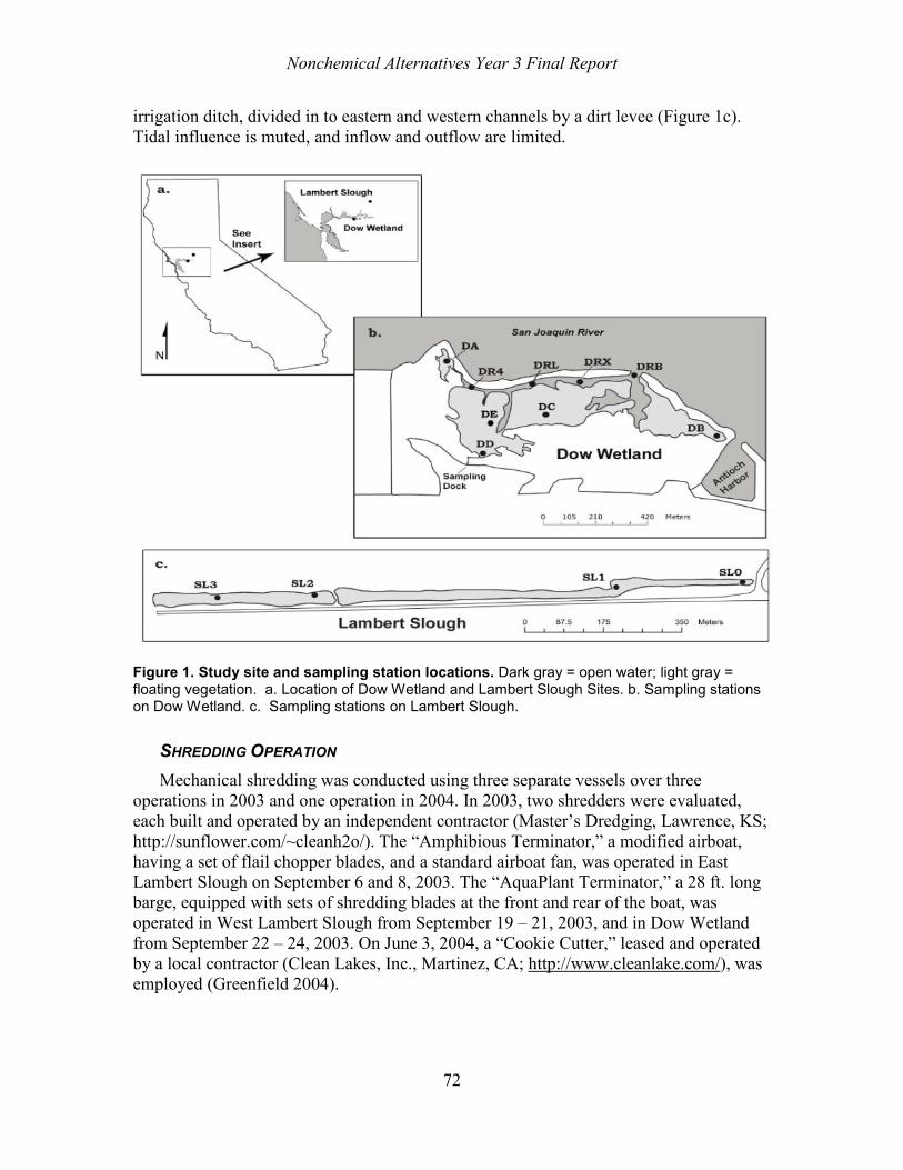
Nonchemical Alternatives Year 3 Final Report
72
irrigation ditch, divided in to eastern and western channels by a dirt levee (Figure 1c). Tidal influence is muted, and inflow and outflow are limited.
Figure 1. Study site and sampling station locations. Dark gray = open water; light gray = floating vegetation. a. Location of Dow Wetland and Lambert Slough Sites. b. Sampling stations on Dow Wetland. c. Sampling stations on Lambert Slough.
SHREDDING OPERATION Mechanical shredding was conducted using three separate vessels over three
operations in 2003 and one operation in 2004. In 2003, two shredders were evaluated, each built and operated by an independent contractor (Master’s Dredging, Lawrence, KS; http://sunflower.com/~cleanh2o/). The “Amphibious Terminator,” a modified airboat, having a set of flail chopper blades, and a standard airboat fan, was operated in East Lambert Slough on September 6 and 8, 2003. The “AquaPlant Terminator,” a 28 ft. long barge, equipped with sets of shredding blades at the front and rear of the boat, was operated in West Lambert Slough from September 19 – 21, 2003, and in Dow Wetland from September 22 – 24, 2003. On June 3, 2004, a “Cookie Cutter,” leased and operated by a local contractor (Clean Lakes, Inc., Martinez, CA; http://www.cleanlake.com/), was employed (Greenfield 2004).

Nonchemical Alternatives Year 3 Final Report
73
CHEMISTRY ANALYSIS In 2003, water quality was collected at one shredding site in Dow Wetland (DD) and
four sites impacted by shredding at Lambert Slough (SL0, SL1, SL2, and SL3). In 2003, four control (unshredded) sites were also monitored at Dow Wetland (DRB, DRL, DRU, DRX) (Table 1). For all sites, sampling was conducted on at least two dates prior to shredding and several dates following shredding. In 2004, it was expected that shredding effects would be more short-lived, and the sampling design was changed to estimate immediate water quality impacts with spatial replication. Specifically, water quality data were collected at four shredding sites in the Dow Wetland (DA, DB, DC, and DD). These data were collected on three dates: June 1 (prior to shredding), June 3 (within one hour following shredding), and June 7 (four days after shredding). Additionally, a datalogging monitor (YSI Sonde 6920) was established to monitor turbidity, dissolved oxygen, and conductivity at 15 minute intervals at one station overlapping the cookie cutter shredding at Dow Wetland, between May 22 and June 25, 2004.
The following parameters were collected for laboratory analysis: total phosphate (TP), dissolved reactive orthophosphate (OP), total Kjeldahl nitrogen (TKN), dissolved nitrate + nitrite (NO3 + NO2), biochemical oxygen demand (BOD), dissolved organic carbon (DOC), total suspended solids (TSS), and turbidity. Single grab samples were collected 0.3 m beneath the water surface in precleaned HDPE-plastic bottles (glass bottles for DOC), and shipped on ice to analytical labs for filtration and preparation within 48 hr. Laboratory analyses were performed using standard EPA and APHA protocols (U. S. EPA 1983, Clesceri et al. 1998). TKN was determined by sulfuric acid digestion followed by boric acid absorption and sulfuric acid titration. NO3 + NO2 was determined colorimetrically, after the reduction of nitrate to nitrite on a copperized cadmium column and subsequent reaction of nitrite with sulfanilamide and N-(1-naphthyl)ethlyenediamine dihydrochloride. Phosphorus was determined colorimetrically, after reduction to molybdenum blue. Prior to analysis, samples for OP were filtered with 0.45 micron filters, and TP samples were digested with sulfuric acid at 115°C. BOD was determined as the depletion of oxygen after five day 20°C incubation. DOC was determined by persulfate ultraviolet oxidation. Turbidity was analyzed using a Hach Model 2100P turbidimeter. Analyses were performed at Sierra Foothill Laboratories (nutrients, BOD, and DOC in 2003; Jackson, CA), California Department of Fish and Game Water Pollution Control Laboratories (nutrients and BOD in 2004; Rancho Cordova, CA), California Laboratory Services (DOC in 2004; Rancho Cordova, CA).
Prior to shredding, total mercury (Hg) analyses were conducted on water, sediment,
and plant samples collected from Dow Wetland site DD (Figure 1b). Water samples were collected in plastic 500 ml acid washed bottles and sediment samples were collected using a 30 cm depth core sampler. Plant samples were collected by hand on April 23, 2004, using plastic gloves and stored in sealed plastic bags. Samples were digested with 30% HNO3 (trace metal grade) and analyzed by cold vapor atomic absorption spectroscopy, using a Perkin Elmer 300 AA spectrophotometer. For all nutrient and Hg analyses, sample QA procedures included field and laboratory duplicates, field and laboratory blanks, laboratory matrix spikes and duplicates, and standard reference materials (Yee et al. 2004).

Nonchemical Alternatives Year 3 Final Report
74
Table 1. Description of shredding and reference sites, including site conditions, cost information, treatment and monitoring dates, andstatistical analyses applied.
Site (Stations) Treatment Treatment Dates Site Conditions Shredded Area (acres)East Lambert Slough (SL0, SL1) Amphibious Terminator 9/6, 9/8/2003 Dense 2' Stem Height 3.5West Lambert Slough (SL2, SL3) AquaPlant Terminator 9/19 - 9/21, 9/26 - 9/27/2003 Dense 3'-4.5' Stem Height 11.7South Stone Lake Amphibious Terminator 9/28 - 9/29/2003 Unknown 1.8Dow Wetland (DD) AquaPlant Terminator 9/21 - 9/24/2003 Dense 4'-4.5' Stem Height 0.9Dow Wetland (DR) 4 Reference Stations None (ref. For 2003) Open WaterDow Wetland (DD) Cookie Cutter 6/3/2004 1' Stem Height 1.3Dow Wetland (DC) Cookie Cutter 6/3/2004 1' Stem Height 0.3Dow Wetland (DB) Cookie Cutter 6/3/2004 1' Stem Height 1.1Dow Wetland (DA) Cookie Cutter 6/3/2004 1' Stem Height 0.6Dow Wetland (DE) Cookie Cutter 6/3/2004 1' Stem Height 0.2
Site (Stations) Water Chemistry Monitoring Dates Chemistry Data Analysis
East Lambert Slough (SL0, SL1) 6/5 - 10/8/2003 Before-After t-test, PCAWest Lambert Slough (SL2, SL3) 8/7 - 10/8/2003 Before-After t-test, PCASouth Stone Lake, Dow (DE) NoneDow Wetland (DD) 8/8 - 11/10/ 2003 a. Before-After t-test, PCADow Wetland (DR) 8/8 - 10/7/2003 Before-After t-test, PCADow Wetland (DA, DB, DC, DD) 6/1, 6/3, 6/7/2004 a. Repeated Measures ANOVA,
PCAAdditional data were collected at site DD: Water Quality in 2002; DO until 2/2004; Mercury in Water, Sediment, Tissues;and Continuous Field chemistry measurement from 5/22 - 6/25/2004

Nonchemical Alternatives Year 3 Final Report
75
STATISTICAL ANALYSIS For 2003 sampling, a number of stations were relatively close to each other (Figure
1), creating the need to evaluate statistical independence for subsequent analyses. Spatial independence of separate sampling stations at each of the two sites (Dow Wetland and Lambert Slough) was ascertained by examining association in water quality parameters measured on the same dates. To limit pseudoreplication, results from separate sites were averaged when Pearson correlation coefficients were above 0.50 for any of the following parameters: BOD, DOC, OP, TKN, turbidity, or dissolved oxygen. Only comparisons having sample sizes of five or more paired samples were used. Once appropriate station partitioning was determined in 2003, it was possible to evaluate treatment effects for individual station categories, combining adjacent stations that were spatially correlated.
Time series data were analyzed for the effect of the mechanical shredding treatment, using a simple independent t-test, comparing samples collected prior to and after the perturbation. Variability of residuals was examined using Levene’s test, and the Welch’s t-test was performed when the residual variances were unequal among treatments (Stewart-Oaten et al. 1992). However, the project involved repeated sampling of individual stations, often with sample sizes (generally between 8 and 12 separate dates) insufficient to effectively address serial autocorrelation, when present (Stewart-Oaten et al. 1992, Rasmussen et al. 2001). Serial autocorrelation of residuals was evaluated by examining autocorrelation and partial autocorrelation functions. If serial autocorrelation was present, and the direction of auto correlation could cause changes in statistical significance (at p < 0.05), t-test results were not included, and interpretations were made based on graphical analysis only.
For 2004, within-station differences in water quality over three sampling dates were
examined using a one-way, repeated measures analysis of variance (ANOVA). All repeated measures F - tests were performed under the assumption of multivariate normality. Mauchly’s Test of Sphericity was used to test for violations of the assumption of sphericity, and probability values adjusted for violations using the Huynh-Feldt epsilon (Von Ende 2001). Metrics were log transformed (metric + 1) to normalize the data and equalize variances.
The datalogging sonde dissolved oxygen and turbidity data exhibited strong daily and
tidal patterns, and mean values were generated for each daily and tidal cycle, based on NOAA predicted tidal patterns for Antioch, CA (http://co-ops.nos.noaa.gov/tides04/tpred2.html).This resulted in sample sizes of 34 days or 66 tidal cycles for each parameter. Data exhibited significant serial autocorrelation (p < 0.05 for the autocorrelation function [ACF]), which needed to be removed prior to evaluation of treatment effects (Rasmussen et al. 2001). Serial autocorrelation was accounted for by evaluating autoregressive (AR) and moving average (MA) models, selecting models based on a combination of factors: successful removal of significant autocorrelation, minimization of the Akaike Information Criterion (AIC) value, and overall model parsimony (minimizing number of parameters) (Box et al. 1994). Serial autocorrelation was present for both daily and tidal results. The residual ACF values remained significant after applying combinations of first and second order AR and MA models to the tidally averaged data. In order to simplify the modeling and interpretation, analyses focused on the daily averaged data, for which

Nonchemical Alternatives Year 3 Final Report
76
serial autocorrelation was readily removed with ARMA techniques. Turbidity data were log transformed to best approximate normal distribution and variance homoscedasticity. The residuals of the time series model were then examined for significant treatment effect using a t-test between samples collected before vs. after shredding. Significance level for all analyses was 0.05.
In addition to examination of individual water quality parameters, overall changes in
water quality were also evaluated, using principal components analysis (PCA). We used PCA to combine the intercorrelated water quality effects into a subset of axes, and graphically evaluate water quality shifts across these axes, in order to ascertain whether shredding impacted the overall water quality of collected samples. PCA was performed on PC-ORD 4.0 software (McCune and Grace 2002) using a correlation coefficient cross-products matrix, as a function of treatment status. Separate PCA were performed for each sampling year, due to differences among years in water quality parameters and sampling designs. Prior to analysis, individual water quality parameters were log transformed when necessary to achieve multivariate normality.
ESTIMATED NUTRIENT MASS RELEASED BY A DELTA WIDE SHREDDING OPERATION To assess the potential ecosystem impact of wide-scale hyacinth treatment on the
Delta, we estimated total hyacinth mass of carbon, nitrogen, and phosphorus. We compared these order of magnitude estimates to the total estimated nutrient mass in the Delta water column, in order to determine whether particular biogeochemical impacts of the treatment method would likely affect overall water quality and the Delta or other similar ecosystems. Mass was separately calculated as the total available mass in plant tissue and the total mass transferred to the water column within several weeks of mechanical shredding. Nutrient release was based on volumetric concentration changes observed in this study, station depth, and Delta wide hyacinth area coverage. Jassby and Cloern (2000) estimated aerial coverage to be 302 ha, based on median area chemically treated from 1983 to 1998. However, the California Department of Boating and Waterways (CDBW) indicate that aerial coverage has increased substantially over the past several years due to chemical treatment permitting difficulties, resulting in current aerial coverage estimates of 1200 to 2200 ha (California Department of Boating and Waterways 2004; A. Morrill, CDBW, pers. comm.). Our modeling exercise therefore spanned the range from 300 to 2200 ha (Table 2).
Calculated hyacinth nutrient mass was compared to an estimated present mass in the
water column. Total Delta water column nutrient mass was estimated as the product of total water volume in the Delta and average water column concentration (Table 2). Total Delta water volume was obtained from N. Monsen (USGS, pers. comm.), using bathymetry in a Delta hydrodynamic model (Monsen 2001). Concentration data was obtained from the publicly accessible Bay Delta and Tributaries (BDAT) database (http://baydelta.ca.gov/). These water quality data are collected by the California Department of Water Resources Estuary Monitoring Project and Municipal Water Quality Investigations programs, and the Port of Stockton’s San Joaquin River Monitoring Program. Data collected from 1995 through 2002 were assembled and

Nonchemical Alternatives Year 3 Final Report
77
averaged by station for dissolved organic carbon (2535 collections at 30 stations), total phosphorus (1487 collections at 38 stations), and TKN (1377 collections at 36 stations). Table 2. Range of values used for estimating total mass of mercury, carbon, nitrogen, and phosphorus in Delta water hyacinth, mass released by a large-scale shredding operation, and mass of nutrients currently in the Delta water column.
E. Crassipes Parameter Value Reference Standing crop (biomass/unit area)
1.8 - 4.3 kg dw/m2
This study
Coverage in Delta 300-2200 ha Jassby and Cloern 2000; CDBW, 2004; A. Morrill, CDBW, pers. comm.
Tissue proportion nitrogen
0.015 - 0.025 Spencer and Ksander 2004 (value for September)
Tissue proportion carbon
0.37 Spencer and Ksander 2004
Tissue proportion phosphorus
0.0022 Klumpp et al. 2002
Tissue proportion mercury
Shoots 0.85 mg/kg dry weight (dw)
Riddle et al. 2002
Roots 4.44 mg/kg dw Riddle et al. 2002 Proportion of hyacinth tissue dry mass in
Leaves 0.3 - 0.6 This study; Penfound, 1948 Stem base and roots 0.4 – 0.7 This study; Penfound, 1948
Delta Water Quality Parameter
Value Reference
Total water volume 1.2 x 10⁹ m3 N. Monsen, USGS, pers. comm. based on Monsen 2001; Kimmerer 2004
Total Kheldal nitrogen 0.78 mg/l See methods Dissolved organic carbon
3.45 mg/l See methods
Total phosphorus 0.19 mg/l See methods Estimated Total Annual Hg Input to Delta (2000)
179.6 kg Foe, 2003
Estimated Total Annual Hg Input to Delta (2001)
98.9 kg Foe, 2003

Nonchemical Alternatives Year 3 Final Report
78
1.3. RESULTS
GENERAL SITE CONDITIONS All shredding locations had dense coverage of water hyacinth, but plant size was
greater when shredding occurred in Fall 2003 than Spring 2004 (Table 1). In September 2003, plant standing crop was 1.8 kg/m2 dry weight in East Lambert Slough (site SL1; SD = 0.4; N = 10) and 4.3 kg/m2 dry weight at Dow Wetland (site DD; SD = 1.3; N = 10) Plant dry weight to fresh weight ratio averaged 0.045 (SD = 0.18; N = 20). In general, each shredding event resulted in a significant reduction in plant standing crop, and number of live plants at a site (e.g., Figure 3c), but many viable fragments remained, and plant regrowth rate was elevated in shredded sites. Overall shredding effectiveness is the subject of separate publications (Greenfield 2004, Greenfield and McNabb 2005, Spencer et al. 2005).
Measured total Hg concentrations in water hyacinth collected from site DD were 1.17
µg/g wet weight in hyacinth roots (SD = 0.08; N = 3 samples), 1.03 µg/g wet weight in hyacinth shoots (SD = 0.52; N = 3), and 0.27 µg/g in sediments (SD = 0.075; N = 10). Of nine unfiltered water samples collected at the site, only three had detectable residues of Hg, with concentrations equaling 0.45, 0.52, and 0.77 µg/l. The remaining six water samples were below the detection limit for total Hg (i.e., less than 0.2 µg/l).
In 2003, measured water quality parameters generally were correlated between the two stations in West Lambert Slough (SL2, SL3), and also between the two stations in East Lambert Slough (SL0, SL1). For these pairwise comparisons, correlation coefficients (r) were positive and ranged between 0.59 and 0.99, with the exception of turbidity in East Lambert Slough, which exhibited r = –0.56. Water quality parameters were generally not correlated between West and East Lambert Slough stations for DO, DOC, BOD, OP, or TKN, with –0.49 < r < 0.42. Correlations were found between stations from the separate sloughs for TP (0.62 < r < 0.98) and turbidity (-0.32 < r < 0.66), though the associations were generally driven by a single data point. Given the correlation between the two West Lambert Slough stations, t-tests were performed on the means of these two stations to avoid pseudoreplication. Although East Lambert Slough sites were correlated, one of the two East Lambert Slough stations (SL0) was not included in t-tests because it was only sampled once prior to treatment. Based on the lack of independence between stations within East or West Lambert Slough, averages for each slough were used in the t-test, creating a total of three independent sampling locations for evaluation of shredding impact [East Lambert Slough (i.e., SL1), West Lambert Slough (SL2 and SL3, hereafter combined into SL23), and the Dow Experimental Station (DD)]. A t-test was also performed on the average of the Dow reference stations (i.e., DR) to ascertain whether water quality traits in the wetland change significantly, independent of shredding.
VARIATION IN INDIVIDUAL WATER CHEMISTRY ATTRIBUTES Overall, t-tests indicated significant changes in water quality after shredding at
experimental sites treated with the AquaPlant Terminator (SL23 and DD) and the

Nonchemical Alternatives Year 3 Final Report
79
Amphibious Terminator (SL1) in 2003 (Table 3). Significant (p < 0.05) increases were observed in OP and TP for treatment stations in 2003 (Table 3, Figure 2). DO decreased significantly at site SL1, exhibited no significant trend at site SL23, and increased significantly at site DD. In contrast to treatment stations, the Dow reference stations (DR) did not exhibit changes in DO, OP, or TP (Table 3). Average TKN concentrations were elevated at SL1, SL23, and DD after shredding, though this pattern was only statistically significant at SL23. Average DOC concentrations were also elevated at SL1 and SL23 after shredding, with a statistically significant increase at SL1. Conductance increased significantly at DD, DR, and SL23, suggesting a salinity influx during the experimental treatment (Table 3). Significant serial autocorrelation impeded statistical analysis for four parameter-site combinations: turbidity in DR, TP in both Dow stations, and TKN in DD (Table 3).
Table 3. Water chemistry results in 2003. Average concentrations are presented for each of four stations before and after shredding. DO = dissolved oxygen. TP = total phosphorus. OP = dissolved orthoreactive phosphorus. TKN = total Kjeldahl nitrogen. DOC = dissolved organic carbon. SD = standard deviation. N = number of sampling dates. The last column presents results of the statistical analysis for differences before versus after shredding. Boldfaced results (p < 0.05) indicate a significant difference.
Value Value
Parameter Station Before After Transformation 2 tail t-test
(units) Mean (SD, N) Mean (SD, N) p > t
DO (mg/l) SL1 1.49 (1.25, 5) 0.07 (0.019, 6) Log 0.008
DO SL23 1.32 (0.78, 8) 0.86 (1.07, 4) Log 0.16
DO DD 4.08 (0.75, 4) 5.10 (0.42, 6) Log 0.012
DO DR 6.77 (2.23, 5) 6.00 (0.84, 4) Log 0.60*
Turbidity
(NTU)
SL1 7.5 (3.7, 5) 13.0 (12.7, 6) Sqrt 0.93
Turbidity SL23 24.3 (20.2, 8) 133 (240, 4) 1/Sqrt 0.96
Turbidity DD 33.0 (8.6, 4) 25.1 (25.5, 6) Log 0.17**
Turbidity DR 11.8 (5.8, 5) 6.2 (1.2, 4) NA
TP (mg/l) SL1 0.10 (0.05, 5) 0.48 (0.29, 4) Log 0.009
TP SL23 0.10 (0.05, 6) 0.64 (0.18, 4) 1/Sqrt < 0.001
TP DD 0.13 (0.04, 4) 0.38 (0.41, 6) NA NA
TP DR 0.07 (0.01, 5) 0.07 (0.02, 4) NA NA
OP (mg/l) SL1 0.012 (0.009, 2) 0.16 (0.064, 4) None 0.036
OP SL23 0.017 (0.010, 4) 0.32 (0.28, 4) 1/Sqrt 0.006

Nonchemical Alternatives Year 3 Final Report
80
Value Value
Parameter Station Before After Transformation 2 tail t-test
(units) Mean (SD, N) Mean (SD, N) p > t
OP DD 0.026 (0.008, 3) 0.089 (0.056 6) Log 0.012
OP DR 0.042 (0.010, 3) 0.043 (0.010, 4) None 0.85
TKN (mg/l) SL1 0.76 (0.36, 4) 2.13 (1.44, 4) Log 0.072
TKN SL23 0.61 (0.23, 5) 1.70 (1.16, 4) 1/Sqrt < 0.02
TKN DD 0.57 (0.23, 4) 1.15 (1.25, 6) NA NA
TKN DR ND (NA, 4) ND (NA, 4) NA NA
DOC SL1 3.9 (NA, 1) 21.5 (4.4, 4) None <0.005
DOC SL23 3.9 (0.6, 2) 14.6 (6.7, 4) Arcsin(Sqrt) 0.08
DOC DD 5.0 (0.3, 2) 4.9 (0.6, 6) 1/X 0.71
DOC DR 3.7 (0.8, 2) 3.7 (0.8, 4) Log 0.99
Conductance (umhos/S)
SL1 254 (72, 5) 281 (44, 6) None 0.47
Conductance SL23 158 (12, 8) 249 (35, 4) 1/X < 0.0001
Conductance DD 1219 (530, 4) 3250 (244, 6) Arcsin(Sqrt) < 0.0001
Conductance DR 1226 (531, 5) 3339 (198, 4) Arcsin(Sqrt) < 0.001
* Variances may be unequal (Levene's test p < 0.10); Used Welch ANOVA assuming unequal variances ** Errors not normally distributed. Used Kruskal-Wallis ranked sum evaluation (Wilcoxon) @ Following Priestly (1981) modified t-statistic to correct for serial autocorrelation ND = all samples were below the detection limit (0.5 mg/l) NA = result not available due to insufficient sample size or serial autocorrelation of t-test residuals
Graphical analysis suggested that nutrient increases and oxygen demand at the
individual Lambert Slough Sites (SL0, SL1, SL2, and SL3) were sustained for several weeks after treatment in 2003 (Figure 2). The average TP increase (i.e., average concentration after treatment minus the average concentration before treatment) was high for all stations, equaling 0.38 mg/l at site SL1, 0.54 mg/l at SL23, and 0.25 mg/l at DD. OP also increased: 0.15 mg/l at SL1, 0.30 mg/l at SL23, and 0.063 mg/l at DD. For DOC, BOD, and TKN, an increase was generally observed after treatment, compared to the pretreatment sample (Figure 2). For example, DOC increased 17.6 mg/l at SL1, and 10.7 mg/l at SL23. BOD resulted in anoxic conditions after treatment at site SL1 (Table 3).

Nonchemical Alternatives Year 3 Final Report
81
In 2004, total nutrient concentrations increased immediately after Cookie Cutter treatment, and then declined to pretreatment conditions (Table 4). Repeated measures ANOVA indicated a significant change over the three sampling periods for TKN (F2,6 =5.947, p = 0.038) and TP (F2,6 = 6.312, p = 0.033). The average observed nutrient increase was 0.37 mg/l for TP and 1.3 mg/l for TKN. Concentrations also increased immediately after treatment for TSS and BOD (Table 4), although this trend was not statistically significant after Huynh-Feldt epsilon adjustment for sphericity violation (for TSS, F1,3 = 8.313, p = 0.061; for BOD, F1,3 = 7.569, p = 0.071). No change was observed in dissolved nutrient concentrations (DOC, OP, or NO3 + NO2) or DO (Table 4).
Table 4. Water chemistry results for four stations monitored at Dow Wetland during Cookie Cutter treatment in 2004. Average concentrations are presented for each of the stations before shredding, immediately after shredding, and four days after shredding. SD = standard deviation. Boldfaced results indicate a significant change in that chemistry parameter over the three sampling dates (p < 0.05).
After After Parameter (mg/l) Before One Hour Four Days Average (SD) Average (SD) Average (SD)
Biological oxygen demand (BOD) 1.5 (0) 5.3 (3) 1.5 (0) Dissolved organic carbon (DOC) 2.9 (0.6) 2.5 (0.3) 1.7 (0.8) Dissolved oxygen (DO) 5.2 (1.2) 4.8 (2.6) 4.4 (1.3) Total phosphorus (TP) 0.12 (0.05) 0.49 (0.31) 0.09 (0.02) Orthoreactive phosphate (OP) 0.06 (0.03) 0.02 (0.03) 0.04 (0) Total Kjeldahl nitrogen (TKN) 0.46 (0.14) 1.76 (1.09) 0.43 (0.06) Dissolved nitrates (NO3 + NO2) 0.22 (0.09) 0.26 (0.13) 0.25 (0.09) Total suspended solids (TSS) 22 (14) 321 (259) 13 (9)
DISSOLVED OXYGEN AND TURBIDITY TRENDS Long-term trend data were collected for DO and conductivity from site DD only.
Over three dates in April and May of 2002, DO concentration declined (Figure 3); this coincided with an invasion of water hyacinth into the site (S. Andrews, personal observation). Mechanical shredding on September 22, 2003 resulted in a decline in the number of hyacinth plants present at site DD (Figure 3c). DO generally increased over the course of 25 measurement dates between June 2003 and February 2004 (Figure 3a). There was a significant increase in DO for dates after mechanical shredding occurred on September 22, 2003 (t-test, p = 0.02; no significant serial autocorrelation), with average concentrations increasing from 3.7 to 5.1 over that time period. Conductivity increased between June and November 2003, but declined sharply in February 2004 (Figure 3b).
DO and turbidity were continuously monitored at site DD from May 22 through June
25, 2004 (Figure 4). Significant serial autocorrelation was observed for daily averaged values of both DO and turbidity (N = 34). For DO, the model with the best fit, based on absence of residual autocorrelation, lowest AIC, and high R2 (0.74) was an AR(1) model (i.e., containing a 1st order autoregressive term). For turbidity (log transformed), the best

Nonchemical Alternatives Year 3 Final Report
82
fit (R2 = 0.32) was also achieved with an AR(1) model. No significant difference was observed between pretreatment and post-treatment samples for the model residuals of either DO (t = 1.24; p = 0.23; 31 df) or turbidity (t = - 0.15; p = 0.89; 31 df). For the raw data (Figure 4a, b), DO declined and turbidity increased during the 24 hr immediately following the primary shredding event. Evaluation of the residuals of the AR(1) models confirmed the graphical results. On June 3, the DO residual was 1.46 SD below the mean (probability of selecting a random sample of this value; p < 0.1) and the turbidity residual was 2.79 SD above the mean (p < 0.005).
Figure 2. Results of the water chemistry monitoring over time for Lambert Slough monitoring stations in 2003. The black dashed vertical line indicates the date of amphibious Terminator shredding in East Lambert Slough. The two East Lambert Slough stations are SL0 (circles) and SL1 (triangles). The solid vertical line indicates the date of AquaPlant Terminator shredding in West Lambert Slough. The two West Lambert Slough stations are SL2 (squares) and SL3 (diamonds). Note log axes, plots b and c, and variations in x axis scale.

Nonchemical Alternatives Year 3 Final Report
83
Figure 2 (cont’d). Results of the water chemistry monitoring over time for Lambert Slough monitoring stations in 2003. The black dashed vertical line indicates the date of amphibious Terminator shredding in East Lambert Slough. The two East Lambert Slough stations are SL0 (circles) and SL1 (triangles). The solid vertical line indicates the date of AquaPlant Terminator shredding in West Lambert Slough. The two West Lambert Slough stations are SL2 (squares) and SL3 (diamonds). Note log axes, plots b and c, and variations in x axis scale.

Nonchemical Alternatives Year 3 Final Report
84
Figure 3. Dissolved oxygen, specific conductance, and plant abundance monitoring over time at the Dow Wetland 2003 mechanical shredding station (DD). The black rectangle indicates a time period when water hyacinth invaded the station area (April – May 2002). The black vertical line indicates when mechanical shredding was conducted on the station with that AquaPlant Terminator.

Nonchemical Alternatives Year 3 Final Report
85
Dis
solv
edO
xyge
n(m
g/l)
0
2
4
6
8
10
12
14
5/24 5/31 6/7 6/14 6/21 6/28
Turb
idity
(NTU
)
050
100150200250300350
a
b
6/3 6/4 6/5
50
150
250
6/3 6/4 6/5 0
3
6
9
Figure 4. Continuous monitoring of the Dow Wetland DD shredding station during a one month period in 2004. The vertical hash lines indicate points when mechanical shredding was conducted on the site using the cookie cutter. Inset plots present on an expanded time scale the 48 hr period when the shredding operation was conducted, with the circled area referred to in the text. a. Dissolved oxygen (mg/l). b. Turbidity (NTU).
OVERALL VARIATION IN CHEMISTRY WITH SHREDDING Principal components analysis was performed on the water quality results of nine
2003 sampling locations, each sampled on four to eight separate dates, resulting in a total of 60 data points. For eight water quality parameters (TP, OP, TKN, temperature, pH, DO, conductivity, and turbidity), the first and second axes explained 41.7 and 28.6 percent of the variance, respectively, totaling 70.3 percent. DO, pH, and conductivity had negative eigenvectors for axes 1 and 2. Nutrient parameters (OP, TP, and TKN) exhibited positive eigenvectors for axis 1 and negative eigenvectors for axis 2 (Figure 5).
Data points fell into distinct clusters on the first two axes as a function of both water
body (Dow Treatment, Dow Reference, Lambert Slough) and treatment (i.e., pretreatment vs. posttreatment) (Figure 5). Lambert Slough samples shifted in the direction of the nutrient and turbidity eigenvectors, suggesting that shredded sites increased in overall nutrient concentrations and turbidity. The Dow treatment samples (DD) decreased along axis 2 after shredding, with increased variability along axis one, suggesting variable and inconsistent water quality changes. Dow reference stations

Nonchemical Alternatives Year 3 Final Report
86
shifted in the direction if increased conductivity and DO, suggesting an influx of saline water, independent of the shredding operation.
Principal components analysis was also performed on the water quality results of four
2004 sampling locations, each sampled on three dates, resulting in a total of 12 data points. For ten water quality parameters (TP, OP, TKN, NO3 + NO2, DOC, temperature, pH, DO, conductivity, and turbidity), the first and second axes explained 41.5 and 26.9 percent of the variance, respectively, totaling 68.4 percent. Total nutrients (TP, TKN, TSS) were strongly correlated, exhibiting a negative eigenvector for axis 1. In contrast, dissolved nutrients exhibited positive eigenvectors for both axes (Figure 6). Data points fell into three fairly distinct clusters according to sample date. The sample event prior to shredding (open symbols) was generally positive for both axes, suggesting elevated DO and dissolved nutrients. Immediately after shredding, three of the four stations (stations DA, DB, and DD) dropped in axis 1, indicating an increase in total nutrients and suspended solids. By the third sample date, samples increased again in axis 1 but declined in axis 2, suggesting a return to pretreatment nutrient conditions but an increase in conductivity.
ESTIMATED NUTRIENT MASS RELEASED BY A DELTA WIDE SHREDDING OPERATION Using compiled data for the Delta, the average TP, TKN, and DOC concentrations
were 0.19, 0.78, and 3.5 mg/l, respectively. These concentrations are comparable to Delta concentrations reported elsewhere (e.g., Jassby et al. 2002, Sobczak et al. 2002, Schemel et al. 2004). For carbon, nitrogen, and phosphorus, the range of estimated total biomass present in water hyacinth tissue spanned the estimated current mass in the Delta water column (Table 5). However, based on concentration increases resulting from the shredding experiments, the maximum possible nutrient releases due to Delta wide shredding operations would be only 3.1% to 8.5% of the mass present in the water column at a given time (Table 5). The total mercury mass present in water hyacinth in the Delta in a given year was estimated to be between 17 and 50 kg. This value is between 10 and 50 % of the estimated annual riverine mercury load to the Delta in 2000 (180 kg) and 2001 (99 kg). Table 5. Potential impact of large-scale shredding operation on Delta nutrient budget, based on study results and compiled data (Table 1, Table 2). Total hyacinth biomass = total biomass of water hyacinth currently present in the Delta in the form of organic carbon, nitrogen, or phosphorus (range of values in metric tons, T). Shredding material released = total amount of shredded material released into the water column, based on study results (Table 2). Current mass in water column = total present mass of nutrients in entire Delta water column; carbon as dissolved organic carbon and nitrogen as total Kjeldahl nitrogen. Maximum shredding addition = maximum percent increase in nutrient as a result of Delta wide shredding operation.
Estimate Carbon Nitrogen Phosphorus Total hyacinth mass (T) 1,940 – 32,600 78.8 - 2200 11.6 – 194 Shredding material released (T) 16 – 352 0.9 – 29 0.4 – 12 Current mass in water column (T) 4,100 940 230 Maximum shredding addition (%) 8.5 % 3.1 % 5.3 %

Nonchemical Alternatives Year 3 Final Report
87
PC Axis 1
-4 -2 0 2 4-4
-2
0
2
4
TPOP
TKN
T
DO/pHC
Turbidity
Figure 5. Results of principal components analysis (PCA) of 2003 water quality sampling data. Gray symbols = before shredding. Black symbols = after shredding. Diamonds = Lambert Slough sites (SL0, SL1, SL2, SL3). Triangles = the Dow treatment site (DD). Circles = Dow reference sites (DDB, DDX, DDL, DDU). Abbreviations indicate eigenvector relative locations for the eight chemistry parameters used in the analysis. C = conductance; DO/pH = dissolved oxygen and pH (locations are almost identical); T = temperature; OP = dissolved orthoreactive phosphorus; TP = total phosphorus; TKN = total Kheldal nitrogen.
PC Axis 1
-4 -2 0 2 4
PCA
xis
2
-4
-2
0
2
4
OP
TSSTP
TKN
T DOpH
C
DOC
NOx
Figure 6. Results of principal components analysis (PCA) of 2004 water quality sampling data. White symbols = pretreatment sampling date. Black symbols = immediately after shredding. Gray symbols = four days after shredding. The different shape samples indicate the four shredding locations monitored in 2004 (DA, DB, DC, DD). The abbreviations in the figure indicate eigenvector relative locations for the ten chemistry parameters used in the analysis. DO = dissolved oxygen; NOx = nitrate + nitrite; TSS = total suspended solids; DOC = dissolved organic carbon; other abbreviations as in Figure 5.

Nonchemical Alternatives Year 3 Final Report
88
1.4. DISCUSSION
Our results indicated increases in water column nutrients, DOC, and BOD, resulting from mechanical shredding of water hyacinth. However, the extent and duration of these effects varied considerably among the different shredding operations; changes were generally greater at the irrigation ditch (Lambert Slough) than the tidal wetland (Dow Wetland), and were more apparent during the Fall 2003 operations, when plants were larger.
Previous studies have shown limited effects of harvesting operations on immediate
water quality (Carpenter and Gasith 1978, Madsen et al. 1988). Shredding without harvesting has been undertaken rarely, due to concerns about organic material inputs into the water column resulting in increasing dominance of undesirable phytoplankton (Scheffer et al. 1993), and further spreading of the macrophyte infestations (Methé et al. 1993, Madsen 1997). Nevertheless, mechanical shredding may be appropriate for circumstances where harvesting is simply too costly and chemical treatment is viewed unfavorably by the public.
Observed nutrient increases were greater at the Lambert Slough site than Dow
Wetland. This likely resulted from the substantial differences in water residence times among these two locations. In 2003, substantial oxygen demand was apparent at one of the Lambert Slough sites (East Lambert Slough), with the site going completely anoxic for several weeks after shredding. On September 24, 2003, 16 days after shredding occurred, about 20 dead bluegill sunfish and one dead carp were observed along the banks of the East Lambert Slough (B. Greenfield, personal observation). Presumably, the anoxic conditions resulted in this fish kill. Lambert Slough exhibits limited flow-through and weak tidal influence, with water exchange occurring via small drainage pipes on the west end of the Slough. In stagnant locations, such as Lambert Slough, shredding would result in decomposition of organic carbon and anoxia, leading to fish mortality (Rahel 1984, Killgore and Hoover 2001), and production of bioavailable methyl mercury (Kelly et al. 1997).
At Dow Wetland, DO concentrations declined during the water hyacinth invasion in
Spring of 2002, and then increased after hyacinth was shredded in Fall of 2003. The Dow Wetland is directly off the mainstem San Joaquin River, experiencing four to six ft. tide height variation, with the complete dewatering of many locations during low tides. The negative association between water hyacinth presence and water column DO likely resulted from the ability of the dense floating vegetation to impede wind and tidal mixing (Madsen 1997, James et al. 2002). By breaking the barrier of floating vegetation, thereby allowing wind-driven and tidal circulation, shredding may increase DO (James et al. 2002), and also increase available habitat for sensitive fish species, such as the Sacramento splittail and chinook salmon (Moyle et al. 2004).
In Spring of 2004, when hyacinth stands were chopped with the Cookie Cutter, water
quality impacts were short lived. At three monitoring stations, TSS, TKN, and TP increased, and DO decreased immediately following shredding, but returned to pretreatment conditions within three days. At the fourth station (DC), where water

Nonchemical Alternatives Year 3 Final Report
89
column nutrient concentrations did not increase, strong winds blew shredded plants and suspended solids towards the shoreline at the time of shredding (B. Greenfield, personal observation), suggesting that the localized shredding impacts were rapidly dispersed. Continuous water quality monitoring at the DD station indicated that a decline in DO and increase in turbidity only persisted for a single tidal cycle. These findings suggest that spring treatments by the Cookie Cutter are likely to have fewer water quality impacts, presumably because the plants are smaller and much less dense early in the growing season (Penfound and Earle 1948, Bock 1969, Spencer and Ksander 2005).
Due to the difficulty obtaining simultaneous measurements at untreated control sites,
statistical treatment-control comparisons (e.g., BACI or related designs, Stewart-Oaten et al. 1992) could not be achieved in this study. Rather, a “weight of evidence” approach must be used to confirm that chemistry changes observed in this study resulted from shredding, rather than unrelated changes in background conditions. In this study, nutrient concentration increases were observed after four separate shredding events (Table 1), indicating that the pattern was robust to different environmental settings and shredding boats. A set of control sites during one of the shredding operations (the Dow Wetland reference stations) did not exhibit changes in nutrient concentrations. The major confounding variable was a conductivity increase during the Dow Wetland experiments, suggesting an influx of saline water from downstream within the Estuary, due to variations in tide strength and riverine inputs (reviewed in Kimmerer 2004). Since, the primary exogenous nutrient sources to the Delta are upstream tributary inputs (Jassby and Cloern 2000), and total organic carbon generally decreases with increasing salinity (Murrell and Hollibaugh 2000), the influx of saline water may in fact account for the short duration of the nutrient loading and oxygen depletion during the Spring 2004 shredding trial. In tidally influenced systems such as Dow Wetlands, local impacts of mechanical shredding are not likely to be a major management concern.
Although the shredding operation generally caused significant increases in water
column DOC, TP, OP, and TKN at the monitoring stations, effects to Delta-wide nutrient budgets would be modest. Assuming high-end estimates for total acreage shredded, the pool of DOC that would be added to the water column is less than 10% of currently present carbon. This suggests that there will be relatively limited impact on formation of trihalomethane and other water treatment contaminants (Fujii et al. 1998, Brown 2003). This result also suggests that shredding operations alone would not ameliorate reduction in pelagic primary and secondary productivity due to carbon declines (Jassby et al. 2002), unless efforts were made to release additional carbon by grinding the plant material into smaller pieces, or shredding was combined with additional management actions. Nevertheless, pelagic metabolism is most strongly influenced by abundance of bioavailable (i.e., labile) organic carbon, such as that produced by phytoplankton, and the majority of Delta carbon is not readily utilized by primary consumers (Jassby and Cloern 2000, Sobczak et al. 2002). It may be beneficial to evaluate whether the pool of carbon produced by shredding hyacinth would be readily utilized by primary consumers, as well as whether it has a high potential for forming chlorination byproducts.

Nonchemical Alternatives Year 3 Final Report
90
Our study, combined with other published studies, does not support the contention that large-scale shredding operations would adversely impact Delta water quality or ecosystem function. Nitrogen and phosphorus are not limiting nutrients (Jassby et al. 2002), and shredding would not cause substantial increases in these nutrients. However, shredding might have adverse impacts in localized areas. These include large inputs of DOC at culinary water canal intakes, as well as increased biological oxygen demand to localized anoxic zones. In particular, the Stockton Deepwater Shipping Canal is impaired due to DO loss (Lehman et al. 2004), and management activities there should focus on reducing oxygen demand.
This and other studies indicate that a relatively high mass of total Hg may be found in
Delta water hyacinth, compared to bed sediments, water, and upstream loads. Furthermore, some evidence exists that sediments beneath hyacinth may contain elevated concentrations of bioavailable methyl-Hg (Ramlal et al. 2003) and sulfate-reducing bacteria (which engage in Hg-methylation) (Gilmour et al. 1992, Muyodi et al. 2004). Furthermore, in laboratory experiments, shredded hyacinth had higher rates of mercury methylation than intact plants (J. Andrews, manuscript in preparation). Thus, mechanical harvesting of water hyacinth may be an appropriate method for mercury remediation in highly contaminated locations (Riddle et al. 2002). Conversely, control methods that allow hyacinth to decay in the water column (e.g., chemical pesticide application or mechanical shredding without removal) could augment mercury methylation and release into the water column. Locations impacted by both mercury contamination and introducted aquatic plants include the Sacramento-San Joaquin River Delta (Bock 1969, Davis et al. 2003), the Florida Everglades (Duvall and Barron 2000, Pimentel et al. 2000), Lake Victoria (Ramlal et al. 2003, Ogwang and Molo 2004), and many small lakes in northern Wisconsin and Minnesota. Therefore, the relative impact of different introduced plant treatment methods on mercury cycling and bioavailability merits further research.
Aquatic macrophytes can be a significant source of internal nutrient recycling in
water bodies, responsible for over 20% of total nitrogen and phosphorus loading (Carpenter and Adams 1977, James et al. 2001), and increasing available nutrients to the pelagic zone. Macrophyte management to reduce eutrophication has included both repeated harvesting to remove bioavailable nutrients (Carpenter and Adams 1978), and encouraging development of macrophyte beds (Scheffer et al. 1993). Since macrophyte beds can trap nutrients, reduce turbidity, and protect algae-grazing zooplankton from fish predation, physical disturbance of macrophyte beds by benthic fish or other mechanisms may cause a water body to rapidly and dramatically shift to a more turbid, phytoplankton dominated state (Scheffer et al. 1993). In the Sacramento-San Joaquin Delta, macrophyte shredding could potentially be used as a method to help increase water column nutrient and organic carbon concentrations, which appear to limit pelagic primary and secondary production (Kimmerer and Orsi 1996, Kimmerer 2002, Sobczak et al. 2002). Our field study indicated significant inputs of nutrients at shredding locations, and we estimated that floating hyacinth contain a biomass of nutrients similar in scale to that currently found in the Delta water column. We estimated that wide-scale shredding has the potential to increase water column carbon by up to 8 %. This action could be combined

Nonchemical Alternatives Year 3 Final Report
91
with other management actions to increase plankton and fish production, including managed flooding of riparian areas, and minimizing fish entrainment mortality at water pumping plants (Moyle et al. 2004, Schemel et al. 2004).
ACKNOWLEDGEMENTS
The following people provided invaluable assistance with field operations and lab analysis in this study: Dave Crane and Martice Vasquez of CDFG-WPCL; John Ross, Geoff Siemering, Marion Wittmann, Nicole David, Kristen Larned, Jennifer Hayworth, and Lester McKee at SFEI; Adrian Down, Kathy Tung, and other students in the UC Berkeley Environmental Science Teaching Program; Sandy and Richard Nurse, and Dale Gimble of Sierra Foothill Laboratories; Adam Daly, Adam Hackett, and Mike Hsu, of CSU-Hayward; Krist Jensen, site manager at Dow Wetland; David Penny and the Masters Dredging Crew; Tom Harvey and Clay Courtright of Stone Lakes National Wildlife Refuge; Tom McNabb and Arturo Florez of Clean Lakes, Inc.; Cynthia Gause, Adam Morrill, and Tim Artz of CDBW; and Ted Schroeder. This study was funded by the California State Water resources Control Board as part of a legal settlement with California Waterkeepers. The authors alone are responsible for statements made in this paper.
REFERENCES
Anderson, L. W. J. 1990. Aquatic weed problems and management in western United States and Canada. Pages 371-391 in A. J. Pieterse and K. J. Murphy, editors. Aquatic Weeds: The Ecology And Management Of Nuisance Aquatic Vegetation. Oxford University Press, Oxford, England
Bock, J. H. 1969. Productivity of the water hyacinth Eichhornia crassipes (Mart.) Solms. Ecology 50:460-464
Box, G., G. M. Jenkins, and G. Reinsel. 1994. Time Series Analysis: Forecasting and Control, 3rd Edition edition. Prentice Hall
Brown, L. R. 2003. Potential effects of organic carbon production on ecosystems and drinking water quality. Issues in San Francisco Estuary Tidal Wetlands Restoration. San Francisco Estuary and Watershed Science 1.http://repositories.cdlib.org/jmie/sfews/vol1/iss1/art3
California Department of Boating and Waterways. 2004. Water Hyacinth Control Program Executive Summary. Pages 1-10 in Water Hyacinth and Egeria densa 2004 Task Force Meeting, Sacramento, CA
Callaway, J. C., and M. N. Josselyn. 1992. The introduction and spread of smooth cordgrass (Spartina alterniflora) in South San Francisco Bay. Estuaries 15:218-226
Caraco, N. F., and J. J. Cole. 2002. Contrasting impacts of the native and alien macrophytes on dissolved oxygen in a large river. Ecological Applications 12:1496-1509
Carpenter, S. R. 1980. Enrichment of Lake Wingra, Wisconsin, by submersed macrophyte decay. Ecology 61:1145–1155
Carpenter, S. R., and M. S. Adams. 1977. The macrophyte tissue nutrient pool of a hardwater eutrophic lake: implications for macrophyte harvesting. Aquatic Botany 3:239-255
Carpenter, S. R., and M. S. Adams. 1978. Macrophyte control by harvesting and herbicides: implications for phosphorus cycling in Lake Wingra, Wisconsin. Journal of Aquatic Plant Management 16:20-23
Carpenter, S. R., and A. Gasith. 1978. Mechanical cutting of submersed macrophytes: immediate effects on littoral water chemistry and metabolism. Water Research 12:55-57
Clesceri, L. S., A. E. Greenberg, and A. D. Eaton. 1998. Standard Methods for the Examination of Water and Wastewater, 20th edition. American Public Health Association, American Water Works

Nonchemical Alternatives Year 3 Final Report
92
Association, and Water Environment Federation
Cofrancesco, A. F. 1996. Water hyacinth control program in USA. Pages 153-160 in R. Charudattan, R. Labrada, T. D. Center, and C. Kelly-Begazo, editors. Strategies for Water Hyacinth Control. U.S. Food and Agricultural Organizaiton, Rome, Italy
Craft, C., P. Megonigal, S. Broome, J. Stevenson, R. Freese, J. Cornell, L. Zheng, and J. Sacco. 2003. The pace of ecosystem development of constructed Spartina alterniflora marshes. Ecological Applications 13:1417–1432
Culpepper, M. M., and J. L. Decell. 1978. Field evaluation of the Aqua-Trio system. Technical Report A-78-3, U.S. Army Engineer Waterways Experiment Station, Vicksburg, MS
Davis, J. A., B. K. Greenfield, G. Ichikawa, and M. Stephenson. 2003. Mercury in sport fish from the Delta region (Task 2A). Final Project Report SFEI.http://loer.tamug.tamu.edu/calfed/FinalReports.htm
Duvall, S. E., and M. G. Barron. 2000. A screening level probabilistic risk assessment of mercury in Florida Everglades food webs. Ecotoxicology and environmental safety 47:298-305
Foe, C. 1995. Evaluation of the Potential Impact of Contaminants on Aquatic Resources in the Central Valley and Sacramento-San Joaquin Delta Estuary. Central Valley Regional Water Quality Control Board Report Central Valley Regional Water Quality Control Board, Sacramento, California.SFEI (BG)
Foe, C. 2003. Mercury mass balance for the freshwater Sacramento-San Joaquin Bay-Delta Estuary (Task 1A). Calfed Final Project Report Central Valley Regional Water Quality Control Board, Sacramento, CA.http://loer.tamug.tamu.edu/calfed/FinalReports.htm
Fujii, R., A. J. Ranalli, G. R. Aiken, and B. A. Bergamaschi. 1998. Dissolved organic carbon concentrations and compositions, and trihalomethane formation potentials in waters from agricultural peat soils, Sacramento-San Joaquin Delta, California: implications for drinking water quality. Water-Resources Investigations Report 98-4147, U.S.G.S., Sacramento,
CA.http://water.usgs.gov/pubs/wri/wri984147/
Gilmour, C. C., E. A. Henry, and R. Mitchell. 1992. Sulfate stimulation of mercury methylation in fresh-water sediments. Environmental Science and Technology 26:2281-2287
Greenfield, B. K. 2004. Evaluation of three mechanical shredding boats for control of water hyacinth (Eichhornia crassipes). Ecological Restoration 22:300-301
Greenfield, B. K., N. David, J. Hunt, M. Wittmann, and G. Siemering. 2004. Review of alternative aquatic pest control methods for California waters. Technical Report San Francisco Estuary Institute, Oakland, CA.http://www.sfei.org/apmp/recent_pubs.html#nonchemical
Greenfield, B. K., and T. P. McNabb. 2005. Control costs, operation, and permitting issues for mechanical shredding of water hyacinth: a case study on the Sacramento-San Joaquin Rivers Delta, California. Journal of Aquatic Plant Management In review
Haller, W. T. 1996. Operational aspects of chemical, mechanical and biological control of water hyacinth in the United States. Pages 137-152 in R. Charudattan, R. Labrada, T. D. Center, and C. Kelly-Begazo, editors. Strategies for Water Hyacinth Control. U.S. Food and Agricultural Organizaiton, Rome, Italy
Hyatt, K. D., and J. G. Stockner. 1985. Responses of sockeye salmon (Oncorhynchus nerka) to fertilization of British Columbia coastal lakes. Canadian Journal of Fisheries and Aquatic Science 42:320-331
James, W. F., J. W. Barko, and H. L. Eakin. 2001. Direct and indirect impacts of submersed aquatic vegetation on the nutrient budget of an urban oxbow lake. APCRP Technical Note ERDC TN-APCRP-EA-02, U.S. Army Engineer Research and Development Center, Vicksburg, MS.www.wes.army.mil/el/aqua
James, W. F., J. W. Barko, and H. L. Eakin. 2002. Water quality impacts of mechanical shredding of aquatic macrophytes. Journal of Aquatic Plant Management 40:36-42
Jassby, A. D., and J. E. Cloern. 2000. Organic matter sources and rehabilitation of the Sacramento-San Joaquin Delta (California,

Nonchemical Alternatives Year 3 Final Report
93
USA). Aquatic Conservation: Marine and Freshwater Ecosystems 10:323-352
Jassby, A. D., J. E. Cloern, and B. E. Cole. 2002. Annual primary production: Patterns and mechanisms of change in a nutrient-rich tidal ecosystem. Limnology and Oceanography 47:698-712
Kay, S. H., and S. T. Hoyle. 2001. Mail order, the internet, and invasive aquatic weeds. Journal of Aquatic Plant Management 39:88-91
Kelly, C. A., J. W. M. Rudd, R. A. Bodaly, N. P. Roulet, V. L. St.Louis, A. Heyes, T. R. Moore, S. Schiff, R. Arvena, K. J. Scott, B. Dyck, R. Harris, B. Warner, and G. Edwards. 1997. Increases in fluxes of greenhouse gases and methyl mercury following flooding of an experimental reservoir. Environmental Science & Technology 31:1334-1344
Killgore, K. J., and J. J. Hoover. 2001. Effects of hypoxia on fish assemblages in a vegetated waterbody. Journal of Aquatic Plant Management 39:40-44
Kimmerer, W. J. 2002. Effects of freshwater flow on abundance of estuarine organisms: physical effects or trophic linkages? Marine Ecology Progress Series 243:39-55
Kimmerer, W. J. 2004. Open water processes of the San Francisco Estuary: from physical forcing to biologial responses. San Francisco Estuary and Watershed Science [Online serial] 2:1-142.http://repositories.cdlib.org/jmie/sfews/vol2/iss1/art1
Kimmerer, W. J., and J. J. Orsi. 1996. Changes in the zooplankton of the San Francisco Bay estuary since the introduction of the clam Potamocorbula amurensis. Pages 403-424 in J. T. Hollibaugh, editor. San Francisco Bay: The Ecosystem. American Association for the Advancement of Science, San Francisco, CA
Klumpp, A., K. Bauer, C. Franz-Gerstein, and M. d. Menezes. 2002. Variation of nutrient and metal concentrations in aquatic macrophytes along the Rio Cachoeira in Bahia (Brazil). Environment International 28:165-171
Lehman, P. W., J. Sevier, J. Giulianotti, and M. Johnson. 2004. Sources of oxygen demand in the Lower San Joaquin River, California. Estuaries 27:405-418
Lucas, L. V., J. E. Cloern, J. K. Thompson, and N. Monsen. 2002. Functional variability of habitats within the Sacramento-San Joaquin Delta: restoration implications. Ecological Applications 12:1528-1547
Madsen, J. D. 1997. Methods for management of nonindigenous aquatic plants. Pages 145-171 in J. O. Luken and J. W. Thieret, editors. Assessment and Management of Plant Invasions. Springer, New York
Madsen, J. D., M. S. Adams, and P. Ruffier. 1988. Harvest as a control for sago pondweed (Potamogeton pectinatus L.) in Badfish Creek, Wisconsin: frequency, efficiency and its impact on the stream community oxygen metabolism. Journal of Aquatic Plant Management 26:20-25
McCune, B., and J. B. Grace. 2002. Analysis of ecological communities. MJM Software Design, Gleneden Beach, OR.www.pcord.com
Methé, B. A., R. J. Soracco, J. D. Madsen, and C. W. Boylen. 1993. Seed production and growth of waterchestnut as influenced by cutting. Journal of Aquatic Plant Management 31:154-157
Monsen, N. E. 2001. A study of sub-tidal transport in Suisun Bay and the Sacramento-San Joaquin Delta, California. Ph.D. Stanford University, Palo Alto, CA
Moyle, P. B., R. D. Baxter, T. Sommer, T. C. Foin, and S. A. Matern. 2004. Biology and population dynamics of Sacramento splittail (Pogonichthys macrolepidotus) in the San Francisco Estuary: a review. San Francisco Estuary and Watershed Science 2:Article 3.http://repositories.cdlib.org/jmie/sfews/vol2/iss2/art3
Murrell, M. C., and J. T. Hollibaugh. 2000. Distribution and composition of dissolved and particulate organic carbon in northern San Francisco Bay during low flow conditions. Estuarine, Coastal and Shelf Science 51:75-90
Muyodi, F. J., M. S. T. Rubindamayugi, and A. K. Semesi. 2004. Effect of water hyacinth on distribution of sulphate-reducing bacteria in sediments of Lake Victoria. Water SA 30:421-425.http://www.wrc.org.za/publications_watersa_jul04.htm
Ogwang, J. A., and R. Molo. 2004. Threat of water hyacinth resurgence after a successful

Nonchemical Alternatives Year 3 Final Report
94
biological control program. Biocontrol Science and Technology 14:623-626
Olson, M. H., S. R. Carpenter, P. Cunningham, S. Gafny, B. R. Herwig, N. P. Nibbelink, T. Pellett, C. Storlie, A. S. Trebitz, and K. A. Wilson. 1998. Managing macrophytes to improve fish growth: a multi-lake experiment. Fisheries 23:6-12
Osumo, W. M. 2001. Effects of water hyacinth on water quality of Winam Gulf, Lake Victoria. United Nations University Fisheries Training Program, Reykjavik, Iceland.http://www.unuftp.is/proj01/OsumoPRF.pdf
Penfound, W. T., and T. T. Earle. 1948. The biology of the water hyacinth. Ecol. Monogr. 18:447-472
Pimentel, D., L. Lach, R. Zuniga, and D. Morrison. 2000. Environmental and economic costs of nonindigenous species in the United States. BioScience 50:53-68.http://www.scholar.google.com/url?sa=U&q=http://www.einaudi.cornell.edu/conf/2003/gmopoverty/pdf/pimentel.pdf
Rahel, F. J. 1984. Factors structuring fish assemblages along a bog lake successional gradient. Ecology 65:1276-1289
Ramlal, P. S., F. W. B. Bugenyi, G. W. Kling, J. O. Nriagu, J. W. M. Rudd, and L. M. Campbell. 2003. Mercury concentrations in water, sediment, and biota from Lake Victoria, East Africa. Journal of Great Lakes Research 29:283–291
Rasmussen, P. W., D. M. Heisey, E. V. Nordheim, and T. M. Frost. 2001. Time series intervention analysis: unreplicated large-scale experiments. Pages 158-177 in S. M. Scheiner and J. Gurevitch, editors. Design and Analysis of Ecological Experiments. Oxford University Press, New York
Riddle, S. G., H. H. Tran, J. G. DeWitt, and J. C. Andrews. 2002. Field, laboratory, and x-ray absorption spectroscopic studies of mercury accumulation by water hyacinths. Environmental Science and Technology 36:1965-1970
Scheffer, M., S. H. Hosper, M.-. Meijer, B. Moss, and E. Jeppesen. 1993. Alternative equilibria in shallow lakes. Trends in Ecology and Evolution 8:275-279
Schemel, L. E., T. R. Sommer, A. B. Muller-Solger, and W. C. Harrell. 2004. Hydrologic
variability. water chemistry, and phytoplankton biomass in a large floodplain of the Sacramento River, CA, U.S.A. Hydrobiologia 513:129-139
Sobczak, W. V., J. E. Cloern, A. D. Jassby, and A. B. Muller-Solger. 2002. Bioavailability of organic matter in a highly disturbed estuary: the role of detrital and algal resources. Proc. Nat. Acad. Sci. USA 99:8101-8105
Spencer, D. F., and G. G. Ksander. 2004. Do tissue carbon and nitrogen limit population growth of weevils introduced to control Waterhyacinth at a site in the Sacramento-San Joaquin Delta, California? Journal of Aquatic Plant Management 42:45-48
Spencer, D. F., and G. G. Ksander. 2005. Seasonal growth of water hyacinth in the Sacramento/San Joaquin Delta, California: implications for management. Journal of Aquatic Plant Management In Press
Spencer, D. F., G. G. Ksander, M. J. Donovan, P. S. Liow, W. K. Chan, B. K. Greenfield, S. B. Shonkoff, and S. P. Andrews. 2005. Evaluation of water hyacinth survival and growth in the Sacramento Delta, California following cutting. USDA ARS Exotic and Invasive Weeds Research Unit, Davis, California
Stewart, R. M., and D. McFarland. 2000. Preliminary results on water-chestnut mechanical control evaluations, Lake Champlain, Vermont. Memorandum U.S. Army Engineers Research & Development Center, Vicksburg, MS
Stewart-Oaten, A., J. R. Bence, and C. W. Osenberg. 1992. Assessing effects of unreplicated perturbations: no simple solutions. Ecology 73:1396-1404
Texas Parks and Wildlife Department. 2005. Aquatic plant management in Texas: a guidance document.http://www.tpwd.state.tx.us/fish/infish/vegetation/guiddoc.pdf
Thomas, L., and L. Anderson. 1984. Waterhyacinth control in California. Waterhyacinth Control Program
Toft, J. D., C. A. Simenstad, J. R. Cordell, and L. F. Grimaldo. 2003. The effects of introduced water hyacinth on habitat structure, invertebrate assemblages, and fish diets. Estuaries 26:746-758

Nonchemical Alternatives Year 3 Final Report
95
U. S. EPA. 1983. Methods for Chemical Analysis of Water and Wastewater. EPA-600/4-79-020, U.S. Environmental Protection Agency
U.S. Ninth Circuit Court of Appeals. 2001. Decision on Headwaters, Inc. and Oregon Natural Resources Council Action V. Talent Irrigation District. in http://www.pestlaw.com/x/courts/headwaters01.html, San Francisco, CA.http://www.pestlaw.com/x/courts/headwaters01.html
Von Ende, C. N. 2001. Repeated-measures analysis: growth and other time dependent measures. Pages 134-157 in S. M. Scheiner and J. Gurevitch, editors. Design and Analysis of Ecological Experiments. Oxford University Press, New York
Yee, D., G. Siemering, J. Hayworth, D. Oros, S. Lowe, and J. Davis. 2004. Aquatic Pesticide Monitoring Program Quality Assurance Program Plan. San Francisco Estuary Institute, Oakland, CA.http://www.sfei.org/apmp/reports/APMP2003QualityAssur.pdf
FOOTNOTES 1 San Francisco Estuary Institute 7770 Pardee Lane Oakland, CA 94621 [email protected]
2 California State University 25800 Carlos Bee Boulevard Hayward, CA 94542
3 Environmental Sciences Teaching Program University of California 301 Campbell Hall MC 2922 Berkeley, CA 94720-2922
4 USDA ARS Exotic & Invasive Weeds Research Unit Plant Science Department University of California One Shields Avenue Davis, California 95616

Nonchemical Alternatives Year 3 Final Report
96
CHAPTER 5 FRAGMENT PROPAGULES OF SPARTINA ALTERNIFLORA & POTENTIAL
EASTERN PACIFIC DISPERSAL Vanessa Howard1 and Mark Sytsma1
ABSTRACT
Commonly used mechanical control methods for Spartina alterniflora involve varying levels of disturbance to rhizomes and roots. We examined the viability of rhizome frag-ments and their potential role in dispersal. Production of rhizome fragments by rototilling in Willapa Bay, Washington was studied. The top 10 cm of the sediment contained an aver-age of 310 fragments/meter2. Median rhizome length was 3.7 cm. Eighty-seven percent of the rhizome fragments had at least one vegetative shoot attached. Survivorship of S. al-terniflora rhizome fragments from Willapa Bay and San Francisco Bay populations was investigated using a three-way factorial design. Treatments included two fragment sizes, approximating those found in Willapa Bay, immersed in freshwater, 15 ppt or 35 ppt salt-water for 3, 8 or 15 days. Fragments were then individually planted and grown in green-house ponds for four months. Rhizome survivorship was low (8.6% or less) in all 35 ppt treatments. Survivorship was 37.3 and 87.5% in 15 ppt and freshwater treatments, respec-tively. Large rhizomes had higher survivorship than small rhizomes at all salinities. The length of time the rhizome fragments were immersed prior to planting had variable effect on survivorship. Results suggest rototilling for control of Spartina may spread the infesta-tion within an estuary but is unlikely to result in spread to other estuaries by ocean trans-port. Thus, tilling should be used with caution in estuaries with small, isolated populations of Spartina.
Although ocean transport of rhizome fragments appears to be a small risk, ocean trans-port of wrack and viable S. alterniflora seed is likely. A drift card study was begun in late September 2004 with the goal of better understanding potential dispersal from invaded west coast estuaries. Monthly releases of cards from Humboldt and San Francisco bays in Cali-fornia, as well as Willapa Bay, Washington will aid identification of wrack deposition sites. Data from the first two months of this year-long study indicate that long-distance dispersal up to 270 km over a four-week period can occur.
Keywords: Spartina alterniflora, rhizome fragment, propagule dispersal, drift card
1.1. INTRODUCTION
Effective invasive plant management considers potential vectors of propagules as well as how to minimize propagule production. In the case of Spartina alterniflora, early detection and treatment efficacy are high priorities for many stakeholders wanting to pre-serve historic habitat, indigenous species, and other beneficial uses of mudflats and native salt marshes in the Pacific Northwest. Within the core infestation sites, thousands of hec-tares have already been colonized including over 790 net hectares (1,960 acres) in San Francisco Bay, California (Zaremba and McGowan 2004) and 3,200 net hectares (8,000

Nonchemical Alternatives Year 3 Final Report
97
acres) in Willapa Bay, Washington. Additionally, thousands of hectares in thirty-one Pa-cific estuaries are at risk for future colonization by one or more invasive Spartina spp. (Daehler & Strong 1996; Pfauth et al. 2003). In Oregon alone, approximately 13,622 hectares (33,660 acres) of intertidal mudflats and aquatic beds are vulnerable to invasion (Pfauth et al. 2003). Understanding both the potential risks and the efficacy of any con-trol method is critical to refining management choices and early detection efforts.
Efficacy and cost data have been evaluated for a wide array of chemical and me-
chanical treatments, (Patton 2002, Hedge et al. 2003, Pfauth et al 2003) however the risk assessments have focused on non-target effects of chemical controls. Mechanical treat-ments such as rototilling, disking, crushing, pulverizing and digging have been problem-atic due their slow pace, variable efficacy, and high cost per area treated (Patton 2002). Yet rototilling and disking are still utilized in some situations to facilitate the decomposi-tion of below-ground biomass, which allows for more rapid restoration to usable shore-bird habitat (Patton & Stenvall 2002) and also where landowners oppose chemical treat-ment options.
Cordgrasses are capable of reproducing by vegetative fragments (Landin 1990, Stiller
& Denton 1995, Daehler & Strong 1996, Sayce et al. 1997, Patten & Stenvall 2002). Disturbances to Spartina’s extensive below-ground structure, such as those caused by rototilling, could potentially produce rhizome fragments. While invasive cordgrasses are known for the resiliency of their rhizomes (Reeder & Hacker 2004, Patton 2003), the vi-ability of mechanically produced rhizome fragments and their role in dispersal has not been closely examined, i.e. evidence is anecdotal (Randall & Milne unpublished, Pfauth et al. 2003).
Research has focused on sexual reproductive capacity of Spartina (Broome et al.
1974, K. Sayce 1988, Daehler 1996, Plyer & Proseus 1996, Sayce & Dumbauld 1997, Daehler 1999, Davis et al. 2004), rather than asexual production, since this is considered to be the primary source of new clones (Stiller and Denton 1995, Sayce et al. 1997). Seed as well as rhizome fragments could disperse Spartina locally or across long dis-tances if carried by tides and ocean currents (Daehler and Strong 1996, Stenvall and Pat-ton 2002, Pfauth et al. 2003). Repeated reports of Spartina fragments washing ashore near Ft. Stevens (near Astoria, Oregon) suggest transport of wrack from nearby Willapa Bay, Washington (Grevstad & Graves, pers. comm., Howard et al., unpublished report 2004). Huiskes et al. (1995) collected seeds of S. anglica in floating and standing nets in a tidal salt marsh in the Netherlands. Eighty-eight percent of the seeds collected were captured in floating nets, indicating that tidal transport of seed was primarily on the water surface rather than along the sediment. In an earlier study in the same location, Koutsaal et al. (1987) released dyed sunflower seeds on outgoing and incoming tides to track tidal movement of seeds in the salt marsh. Seeds were found as much as 45 km away within one week of release. The final location of seeds was determined by the wind velocity and direction as well as by tidal currents.
Oregon’s Spartina Response Plan (Pfauth et al. 2003) was developed to prevent the
introduction and spread of any Spartina species in Oregon. Areas requiring further re-
Nonchemical Alternatives Year 3 Final Report
98
search were identified and included clarification of the likelyhood of Spartina fragments to resprout and an examination of potential transport of propagules via ocean transpor.
Preliminary results from three studies addressing these research needs are presented here. Firstly, a field study was performed to assess the production of Spartina fragments by rototillng. Secondly, a greenhouse experiment examined the ability of rhizome frag-ments to resprout. Thirdly, preliminary data from a propagule dispersal study are pre-sented.
1.2. MATERIALS & METHODS
FIELD STUDY OF ROTOTILLING EFFECTS Samples were collected on January 16, 2004 along the south shore of the Naselle
River, which flows into the southeastern end of Willapa Bay, Washington. Staff of Wil-lapa NWR was mechanically treating the site between high tides with the Wilco am-phibious vehicle and the rear-towed rototilling attachment. The Wilco operator made single passes within a solid meadow of Spartina alterniflora and tilled to a depth of ap-proximately 15 centimeters. Immediately following rototilling, three quadrats (0.25 m2)were haphazardly chosen approximately thirty meters apart and excavated to a depth of 10 cm. Excavated material was rinsed clean and all fragments were measured for culm length, number of culms, and rhizome diameter and length. Fragments were divided into two rhizome sizes, small and large, by the median value for rhizome length. The mean value of each of these rhizome class sizes was then rounded to the nearest half centimeter and used as the experimental rhizome sizes for the greenhouse study of fragment viabil-ity.
GREENHOUSE STUDY A 2x3x3 factorial design was used to evaluate survivorship of S. alterniflora frag-
ments. Factors were initial rhizome size (large or small), immersion duration (three, eight or fifteen days), and salinity (freshwater, 15 ppt, or 35 ppt). Samples from two populations were compared. Rhizome fragments from San Francisco were collected on March 26, 2004 from the shoreline of Elsie Roemer Bird Sanctuary on Alameda Island (San Francisco, California). S. alterniflora at this site had previously been identified as pure S. alterniflora – rather than the more locally common S. alterniflora x S. foliosa hy-brid (D. Ayres, UC Davis, personal communication). Two to three samples were dug from each of ten clones. Samples from Willapa Bay were collected on April 5, 2004 from four riverbank locations (two along the Naselle River, one on the Niawiakum River, and one on the Palix River). Seven to ten samples were dug from each location. Sam-pling locations had not been subjected to any previous chemical or mechanical treatment.
Samples were returned to Portland State University and rinsed clean of all mud and
organic matter within two days of field collection. Within twenty minutes of rinsing, fragments were cut to fit one of two rhizome class sizes (large ~7.5 cm or small ~2.5 cm). Fragments were then placed in open plastic tubs containing water at 0 ppt, 15 ppt or 35 ppt (Instant Ocean® aquarium salts). Tubs were maintained under ambient greenhouse conditions. Salinity concentrations were monitored daily and adjusted with fresh water as

Nonchemical Alternatives Year 3 Final Report
99
needed. After floating for a period of three, eight or fifteen days (referred to as immer-sion duration), each fragment was measured to determine rhizome length, rhizome di-ameter, number of attached culms and culm length. The 8-day immersion duration was eliminated from the San Francisco treatment design due to limited plant material. Frag-ments were then individually potted in six-inch diameter pots with a sterile potting me-dium and each pot placed into a wet bed (1.83 x 2.44 m wood-framed beds lined with three layers of 6 mm clear plastic) containing either 0 ppt, 15 ppt or 35 ppt saline water to a depth of 10 cm). A total of 234 fragments, with at least one culm, were potted from the San Francisco samples. A total of 353 fragments, with at least one culm, were potted from the Willapa Bay samples. Each potted fragment was randomly assigned to the same salinity wet bed as it had been exposed to during the immersion duration. A total of six wet beds were created (two at each salinity level) with three utilized for the San Fran-cisco fragments and three for the Willapa Bay fragments. Salinity of the wet beds was monitored every one to three days and adjusted with saline or fresh water as needed.
A total of 234 fragments, all having at least one culm, were potted from the San Fran-
cisco samples. A total of 353 fragments having at least one culm were potted from the Willapa Bay samples. An additional 116 fragments with no culms attached were created from these samples. The purpose of these fragments was to test if survival was depend-ent upon the presence of at least one culm as suggested by Randall & Milne (unpub-lished, 1996). Small and large rhizome fragments were immersed in the saline baths (0 ppt, 15 ppt or 35 ppt) for either 4 or 16 days. The immersion duration treatments for these fragments were extended by 1 day to allow adequate time for planting of the other treatment groups. They were then individually potted in the same sterile potting medium and placed in the wet beds.
Pots were randomly positioned within the wet beds. All plants were exposed to am-
bient light and temperature conditions for 132 days after planting. Survival, culm length and the number of culms were recorded at 30, 51, 74, 95, 116 and 132 days after planting. Survival was defined as the presence of at least one green culm. Roots, rhizomes, culms and inflorescences were separated 132 days after planting and their fresh weight (fw) re-corded. Dry weight (dw) was obtained after drying the roots, culms and inflorescences to a constant weight in the greenhouse and oven drying the rhizomes at 65-70 °C for 48 hours.
PROPAGULE DISPERsAL STUDY Monthly releases of bouyant, biodegradable wooden drift cards began in September
2004, from the mouths of Willapa Bay in Washington and Humboldt and San Francisco bays in California. A total of 600 cards are released each month – 200 each per bay. Re-leases occurred within two hours after high tide to ensure an outgoing current. Each batch of cards is printed with a unique code denoting the location, month and year of the release as well as reporting instructions and contact information. Velocity estimates were made under the assumption that the recovery date was the same as date the card washed ashore and that the card followed a straight line of travel.

Nonchemical Alternatives Year 3 Final Report
100
1.3. RESULTS
FIELD STUDY OF ROTOTILLING EFFECTS This amounted to 310 fragments (± 54.8) per square meter within ten centimeters of
the surface. Of these, 87.7% had at least one culm attached (Table 1). No plant material other than S. alterniflora was present in any of the plots.
One-way ANOVAs (α=0.05) comparing quadrats were performed on rhizome length
and culm length (log(x+1) transformed) and rhizome diameter (square root(x+1) trans-formed and number of culms per fragment. The quadrats did not vary significantly in rhizome length (p=0.240) or the number of culms per rhizome fragment (p=0.322). There were significant differences between quadrats with regard to culm length (p<0.0001) and rhizome diameter (p<0.0001) (Figure 1).
Rhizomes shorter than the median length (3.7 cm) had a mean of 2.4 cm (± 0.73
S.D.). Those larger than the median length had a mean of 7.5 cm (± 2.98 S.D.) (Figure 2). These two mean rhizome sizes, rounded to the nearest half centimeter, were used to define the small and large rhizome classes used for the greenhouse study.
Table 1: S. alterniflora rhizome fragment metrics following single-pass, winter rototilling effects in Willapa Bay.
Measure Mean ± SD Number of fragments per 0.25 m2 x 0.1m deep 77.7 ± 13.7
Percentage with ≥ 1 culm 87.8 ± 3.86 Rhizome length (cm) 4.96 ± 3.38
Rhizome diameter (cm) 0.58 ± 0.29 Culm length (cm) 5.37 ± 3.58
Culms per fragment 1.31 ± 0.89

Nonchemical Alternatives Year 3 Final Report
101
Quadrat
Rh
izom
eLe
ngt
h(c
m)
321
6.5
6.0
5.5
5.0
4.5
4.0
Quadrat
Rh
izom
edi
amet
er(c
m)
321
0.8
0.7
0.6
0.5
0.4
Quadrat
Cu
lmLe
ngt
h(c
m)
321
8
7
6
5
4
Quadrat
#of
culm
s
321
1.6
1.5
1.4
1.3
1.2
1.1
1.0
Figure 1: Interval plots by quadrat (with 95% C.I.) of rhizome length, rhizome diameter, culm length and number of culms per rhizome fragment found immediately following sin-gle pass, winter rototilling in Willapa Bay, WA.
Rhizome Length (cm)
Freq
uen
cy
1512963
60
50
40
30
20
10
0
7.52.4
Figure 2: Rhizome sizes found immediately following single-pass winter rototilling in Wil-lapa Bay, WA.

Nonchemical Alternatives Year 3 Final Report
102
GREENHOUSE STUDY Survival
No new culms were produced by any of the Willapa Bay (WB) rhizome fragments that were planted without culms. Since survival was defined as the presence of at least one green stem, one-hundred percent of these fragments were defined as dead within the first thirty days of the experiment. Subsequent observations of these fragments showed no signs of culm production. Prior to planting, the position of the fragment within the immersion tubs was observed. While all of the fragments having attached culms re-mained floating after 15 days, only a few of the fragments with no attached culms re-mained floating after 16 days.
The proportion of surviving fragments per treatment group stabilized by the end of the growing period (Figure 3). For San Francisco (SF) plants, survival 132 days after planting ranged from 45 to 100% in the freshwater treatments, 55 to 90.0% in 15 ppt wa-ter and 0 to 5.56% in 35 ppt water. For WB plants, survival ranged from 26.3 to 81.8% in the freshwater treatments, 27.8 to 88.9% in 15 ppt water and 0 to 11.1% in 35 ppt wa-ter.
For nearly all SF groups, rhizomes fragments immersed for three days prior to plant-ing showed lower rates of survival than those immersed for fifteen days (Figure 4). The same pattern emerged with the WB 15 ppt fragments where the three day immersion groups showed much lower survival than the eight immersion groups. Large rhizome fragments consistently had higher viability than small rhizome fragments. For SF plants, 80.3% of large fragments survived compared to only 62.5% of the small fragments. For WB plants, the difference was more pronounced with 74.8 % of large and 36.2% of small fragments surviving. SF and WB populations were compared using a two-tailed test of two proportions; there were significant differences between the proportions surviving in both freshwater (72.5% vs. 55.5% respectively, p=0.012, α=0.05) and 15 ppt water (70.1% vs. 56.0%, p=0.043, α=0.05). In both of these comparisons, SF fragments had higher survivorship. There was no notable difference between the two locations survival rates (3.9% vs. 5.1%) in the high salinity treatment (p= 0.691, α=0.05).

Nonchemical Alternatives Year 3 Final Report
103
San Francisco
020
4060
80100
0 30 60 90 120
days post-planting
%su
rviv
al
Willapa Bay
020406080
100
0 30 60 90 120
days post-planting
%su
rviv
al
Figure 3: Percent S. alterniflora fragment survival over time for a) San Francisco and b) Willapa Bay plants. Treatment groups are noted by salinity (········ 0 ppt, ––––––– 15 ppt and -- –– -- –– 35 ppt), and rhizome size (plain line = small, �= large).
San Francisco
020406080
100
3 day 15 day 3 day 15 day
small large
%su
rviv
al
Willapa Bay
020406080
100
3 day 8 day 15 day 3 day 8 day 15 day
small large
%su
rviv
al
Figure 4: Percent fragment survival 132 days after planting of S. alterniflora from a) San Francisco and b) Willapa Bay. White = 0 ppt, striped = 15 ppt, black = 35 ppt. All fragments represented here were planted with at least one attached culm.
PROPAGULE DISPERSAL STUDY
Drift card return rates have been over 20% for five of the six releases performed as of November 11, 2004 (Table 2). Cards have consistently been found both to the north and south of each release location. In four of the six releases performed to date, cards have been found inside the estuaries. The majority of cards are staying within 25 km of the release locations, although a few have traveled longer distances.
b
a

Nonchemical Alternatives Year 3 Final Report
104
In Willapa Bay, over 69% of the September released cards and 95% of the October released cards were found to the north of the bay. Maximum northward velocities for September and October releases were 6.9 and 11.2 cm/s respectively, while maximum southward velocities reached 6.7 and 3.4 cm/s.
In Humboldt Bay, approximately 72% of the September cards were carried south. Maximum velocity for September release was approximately 3.4 cm/s both to the north and south. Only one card, found after six days and six km north of the Humboldt Bay entrance, was recovered from Humboldt’s October release.
The highest number of cards found within an estuary occurred in the San Francisco September release when thirty cards were recovered on the eastern edge of the bay, mainly near the Berkeley and Albany shoreline. Observed winds at the time of that release were from the west at approximately 7.7 – 10.3 m/s. Recoveries of San Francisco cards not blown back into the bay after the September release showed 61% were carried south. Maximum velocities for this release were approximately 2.4 cm/s to both the north and south. Eighty-seven percent of October cards were found to the south. Maximum velocities were 5.4 cm/s to the north and 6.9 cm/s to the south.
Table 2: Summary data for two months of drift card releases from three S. alterniflora in-fested bays.
Release Date Willapa Humboldt San Francisco September 2004Recovery Rate 57.5% 21.5% 30.5%
Quantity of recovered cards North South Inside bay
79 34 2
10 31 2
12 19 30
Max distance traveled (km) North South
95 35
75 65
45 20
October 2004Recovery Rate 29.5% 0.5% 24.0%
Quantity of recovered cards North South Inside bay
56 30
100
641 1
Max distance traveled (km) North South
223 35
6na
75 30
1.4. DISCUSSION
Rototilling appears to have fairly uniform cutting action on solid meadows; it pro-duces rhizome fragments of consistent size and with similar numbers of attached culms. A high percentage (87.8%) of the S. alterniflora fragments produced by rototilling in Willapa Bay had at least one attached culm. The observed difference in culm length and rhizome diameter between quadrats was likely a result of variations in the age of coa-lesced clones, rather than to variable tearing action by the tilling blades. Assuming uni-formity in the production of rhizome fragments (approximately 312 fragments/m2 within the top ten centimeters) we could make a conservative estimate that 0.5% of fragments might be loosened by wave or tidal action, becoming suspended in the water column. Based on those assumptions, as many as 15,600 fragments might be distributed in the open water for every hectare rototilled (~6,300 per acre).

Nonchemical Alternatives Year 3 Final Report
105
Viability of rhizomes after floating at the water surface seems to be primarily de-pendent on the presence of at least one culm. Randall and Milne (unpublished, 1996) found that rhizome fragments 2.5 to 15 cm long with no attached culms had 100% mor-tality regardless of position on the mud-flat substrate or beneath it at various depths. The presence of attached culms should allow the fragment to respire and thereby increase its chance of survival. In fact, repeated mowing to remove vegetative shoots caused a reduc-tion of oxygen to the root system and was initially utilized as a control method for Spartina (Ebasco Environmental 1993, Hedge et al 1997). Of the 116 rhizomes planted without attached culms during the greenhouse study, none survived. Compared to frag-ments planted with culms, this finding seems to support the theory that at least one vege-tative shoot is needed for survival of vegetative propagules.
For fragments having culms, salinity and initial rhizome size determined survival.
The 35 ppt treatment had notably reduced survival compared to the lower salinity treat-ments. Differences in 0 ppt and 15 ppt treatments appeared largely due to initial rhizome size. Larger rhizomes would logically have higher chances of survival since they would be likely to have more nodes, greater number of established roots and more non-structural carbohydrates to fuel new growth.
The length of immersion was a less important determinant of survival and establish-
ment or rhizome fragments than salinity or rhizome size. Longer immersion durations may increase viability, although this effect was not consistent. Three to four months of wet, cool conditions may help break seed dormancy and increase germination rates by leaching a germination inhibitor. Similarly, the conditions fragments are exposed to while floating in open water may retard growth of pathogens, encourage shoot production or elongation or otherwise increase chances of survival.
Repeated monitoring of treated sites in Willapa Bay has shown that mechanical
treatments such as rototilling and disking have higher efficacy during the period of De-cember through February (Patton & Stenvall 2002). All of the plants used for this study were collected four to five weeks after the normal rototilling period in Willapa Bay. In-creased culm length, as well as higher air, soil and water temperatures at the time of col-lection, may have increased survival rates. Additionally, the vigorous action of rototill-ing produces more ragged edges and somewhat damaged culms than were reproduced in the greenhouse. This might also elevate rates of survival shown here.
Preliminary results from the first two months of the drift card study suggest propagule
deposition from infested estuaries lessens with increased distance. Flow over the coastal shelf is predominantly poleward in the winter and early spring, with mean current veloci-ties of 20 cm/s. Summer time flow is typically southward with mean velocities of 10 cm/s. Dispersal patterns seen from these preliminary findings may be due to a seasonal transition period between these predominant currents. Recovery patterns may also reflect wind forcing and local eddies from the mouths of the release estuaries. Frequent recover-ies in beaches along Long Beach peninsula, where Spartina wrack is commonly found in the fall, suggests that the cards simulate wrack dispersal with some accuracy.

Nonchemical Alternatives Year 3 Final Report
106
1.5. CONCLUSIONS
The estimate of 15,600 fragments per hectare may seem inconsequential when com-pared to estimates of seed germination rates for S. alterniflora which range from nine to nineteen million seeds per hectare (3.7 million to 7.7 million seeds per acre) (Daehler and Strong 1994). However, understanding the risks associated with all control methods is necessary when site-specific treatment decisions are made. Rototilling, or other me-chanical disturbance, producing fragments larger than 2.5 cm should be used with caution in areas with fresh to mesohaline waters. Mechanical disturbance following some other treatment method, such as herbicide application, may pose less of a risk of starting new clones. If the infestation is isolated and/or the population in is not setting seed, caution may be warranted in using rototilling or similar mechanical treatments, since it could produce viable propagules.
A greater understanding of the dispersal patterns from infested bays should help to
identify the risk of seed or vegetative propagule transport. This data, combined known characteristics of susceptible habitat, will help identify natural deposition sites of invasive Spartina spp.
ACKNOWLEDGEMENTS:
Thanks to Debra Ayres, UC Davis Department of Evolution & Ecology, and Erik Gri-jalva, San Francisco Estuary Invasive Spartina Project for their assistance in California; Terri Butler and Jonathan Bates of Willapa National Wildlife Refuge, Fritzi Grevstad and Kim Patton of the University of Washington for their suggestions and field assistance in Washington. For volunteering to release drift cards, we thank David Heimer, Les Hol-comb and Travis Haring of WADFW; Bill Pinnix, USFWS in Arcata, CA and Kristen Ward, NPS Golden Gate Recreation Area. Additionally, the staff and many students at The Center for Lakes & Reservoirs, PSU have been immensely helpful suggestions and field/greenhouse work. This study was funded by the California State Water Resources Control Board, as part of the Aquatic Pesticide Monitoring Program.
REFERENCES
Broome, S.W., W.W. Woodhouse, and E.D. Se-neca (1974). “Propagation of smooth cordgrass, Spartina alterniflora, from seed in North Carolina.” Chesapeake Science15(4): 214-221.
Daehler, C.C. (1999). “Inbreeding depression in smooth cordgrass (Spartina alterniflora,Poaceae) Invading San Francisco Bay.” American Journal of Botany 86 (1): 131-139.
Daehler, C.C. and D.R. Strong (1996). “Status, prediction and prevention of introduced cordgrass Spartina spp. invasions in Pacific
estuaries, USA.” Biological Conservation78: 51-58.
Davis, H.G., C.M. Taylor, J.C. Civille and D.S. Strong (2004). “An Allee effect at the front of a plant invasion: Spartina in a Pacific Es-tuary.” Journal of Ecology 92: 321-327.
Hedge, P., L.K. Kriwoken, and K. Patton (2003). “A review of Spartina Management in Washington State, US.” Journal of Aquatic Plant Management 41: 82-90.
Howard, V., D. Isaacson, and M. Sytsma (2004) “Oregon Department of Agriculture Report: Detection of Spartina spp. on the Oregon Coast in 2003.” Unpublished report. 16 pgs.

Nonchemical Alternatives Year 3 Final Report
107
Huiskes A.H.L., B.P. Koutstaal, P.M.J Herman, W.G. Beeftink, M.M.Markusse and W. De Munck (1995) Seed dispersal of halophytes in tidal salt marshes. Journal of Ecology 83: 559–567
Koutstaal, B.P., M. M. Markusse, and W. de Munck (1987). Aspects of seed dispersal by tidal movements.” Vegetation Between Land and Sea. A.H.L. Huiskes, C.W.P.M. Blom and J. Rozema (eds). Boston, Dr. W. Junk Publishers.
Landin, M. (1990) “Growth habits and other considerations of smooth cordgrass, Spartina alterniflora Loisel.” Spartina Workshop Record. T.F. Mumford Jr., P. Peyton, J.R. Sayce and S. Harbell (eds). Se-attle, WA. 15-20.
Patten, K. and C. Stenvall (2002). “Nothin’ could be fina’ than the killin’ o Spartina.” Agrichemical and Environmental News, Washington State Cooperative Extension Newsletter (196).
Patton, K (2002) “The efficacy of mechanical treatment efforts in 2001 on the control of Spartina in Willapa Bay in 2002.” Progress report to The Willapa National Wildlife Refuge. 20 pgs.
Patton, K. (2003) “Persistence and non-target impact of Imazapyr associated with smooth cordgrass control in an estuary.” Journal of Aquatic Plant Management 41: 1-6.
Pfauth, M., M. Sytsma and D. Isaacson (2003). Oregon Spartina Response Plan. Portland State University, Oregon.
Plyler, D.B. and T.E. Proseus (1996). “A com-parison of the seed dormancy characteristics of Spartina patens and Spartina alterniflora (Poaceae).” American Journal of Botany 83 (1): 11-14.
Randall, P. and D. Milne (1996). “Loose Spartina alterniflora rhizomes don’t sprout new plants.” Unpublished report. Evergreen State College, Washington. 5 pgs.
Reeder, T.G., and S.D. Hacker (2004) “Factors contributing to the removal of a marine grass invader (Spartina anglica) and subse-quent potential for habitat restoration.” Es-tuaries 27 (2): 244-252.
Sayce, K. (1988). Introduced cordgrass, Spartina alterniflora Loisel., in salt marshes and tide-lands of Willapa Bay, Washington. Illwaco, Washington, U.S. Fish and Wildlife Service.
Sayce, K., B. Dumbauld, and J. Hidy. (1997). “Seed dispersal in drift of Spartina al-terniflora.” Second International Spartina Conference, Olympia, WA.
Stiller, J.W. and A. L. Denton (1995). “One hundred years of Spartina alterniflora (Poaceae) in Willapa Bay, Washington: random amplified polymorphic DNA analy-sis of an invasive population.” Molecular Ecology 4: 355-363.
Zaremba, K. and M.F. McGowan (2004) “San Francisco Estuary Invasive Spartina Project Monitoring Report for 2003.” Coastal Con-servancy, October 28 2004.
FOOTNOTES 1 Center For Lakes and Reservoirs Department of Environmental Sciences and Re-
sources Portland State University P.O. Box 751 Portland, OR 97207 [email protected]

Nonchemical Alternatives Year 3 Final Report
108
CHAPTER 6 INSTALLATION OF CREEPING WILDRYE RIPARIAN BUFFER STRIPS
TO CONTROL EROSION ALONG AN IRRIGATION DRAINAGE DITCH Sam Earnshaw1
1.1. INTRODUCTION
Buffer strips alongside waterways can impede the inflow of effluents, thereby reducing eutrophication and growth of aquatic plants. Planting native perennial species at the perimeter of water bodies may aid in the absorption of nutrients. This may also help reduce soil erosion. Riparian buffer strips are also used to control storm water phosphorus loading from residential developments (e.g., Woodard and Rock 1995). The Community Alliance with Family Farmers (CAFF) conducted a demonstration project installing riparian buffer vegetation to improve water quality along an irrigation drainage ditch in the Salinas Valley, California.
1.2. SITE SELECTION AND EVALUATION
In June 2001, CAFF planted 1,200 feet of hedgerow shrubs, herbs and grasses on two waterways that are part of a large conventional vegetable farm operated by Dirk Giannini in the Salinas Valley.
Figure 1. Grasses planted in drainage ditch in June 2001.

Nonchemical Alternatives Year 3 Final Report
109
CAFF contacted the farmer to inquire if there were any more irrigation ditches on his farm that he would like to have vegetated. He expressed interest in vegetating more areas of one of the ditches. Sam Earnshaw , CAFF Central Coast Regional Program Coordinator and Project Manager for this project, visited the site with Dirk, and inspected the proposed planting areas. Dirk had selected four stretches along the ditch, totaling approximately 2000’ in length. Based on the success of the previous planting, the farmer’s desire to install and maintain the planting, and the overall suitability of the ditch to be converted from a bare, weedy, eroding ditch to a vegetated waterway, the site was chosen for the project.
Figure 2. Eroding ditch, before grading, to be planted to grasses.
1.3. SITE ANALYSIS
The site is approximately 2000’ of bare and eroding drainage ditch that runs from the upper stretches of several hundred acres of irrigated lettuce, broccoli and other cool-season vegetables to a large drainage ditch on Old Stage Road, in the Salinas Valley. Approximately 200’ had been planted to perennial grasses and shrubs in 2001, and four stretches of the same ditch totaling approximately 2000’ in length were selected to be planted to perennial grasses. The width of the planting would be approximately 8 feet on each side of the bottom of the ditch. Before the project, the ditch was steep and eroding. For site preparation, the farmer graded the ditch so that the sides were less steep, and it was pre-irrigated.

Nonchemical Alternatives Year 3 Final Report
110
Figure 3. Graded ditch, with trays of grass plugs. The soils are the decomposed granite characteristic of the Salinas Valley south of the
city of Salinas, which are highly erosive. The hydrology of the area is characterized as having both rainfall and irrigation water flowing east toward Old Stage Road and into a large drainage ditch that flows into Quail Creek, then into the Salinas River and ultimately into the Monterey Bay. The ditch to be vegetated is just one of several ditches running east-to-west and draining the farmlands along Old Stage Road.
1.4. PLANNING AND PLANTING
In accordance with typical plantings of the perennial grass, creeping wildrye (Leymus triticoides), it was decided to plant grass plugs at a 6”-12’’ spacing, from the base of the graded ditch to the top of the ditch at the edge of the road. The ditch would be planted on both sides. CAFF got estimates from several nurseries, and contracted in July 2004 with Rana Creek Habitat Restoration, Carmel Valley, California, to grow 146 trays (approximately 20,000 plugs) of creeping wildrye, that would be ready for planting at the end of September.

Nonchemical Alternatives Year 3 Final Report
111
Figure 6. Trays of grass plugs at Rana Creek Nursery. The grasses were picked up and delivered to the farm on September 27, 2004 and
were planted on the same day.
Figure 7. Planting grass plugs, one at a time.

Nonchemical Alternatives Year 3 Final Report
112
Following the planting, the site was irrigated to help the grasses become established.
Figure 8. Planted ditch being irrigated after planting. With the two major rain events that have occurred in October, 2004, irrigation will
probably be unnecessary until the following dry season, when some water will be applied to help the upper plants grow. Once established, irrigation will not be required. The farmer will do periodic weeding, to remove unwanted broadleaf vegetation.
Figure 9. Newly planted grassed waterway.

Nonchemical Alternatives Year 3 Final Report
113
1.5. CONCLUSION
This has been a successful project. Approximately 4000’ of bare and eroding ditch bank has been vegetated with native perennial grass, and the need for applying aquatic pesticides has been eliminated. This planting will serve as a model for other farmers, and will in itself help reduce the pesticides, nutrients and sediments that might enter the Monterey Bay.
The farmer, Dirk Giannini, requests that he be contacted in advance at (831) 449-
2494 to request permission for any proposed visit to the site, and that no pictures or videos be taken without permission.
REFERENCES
Woodard, S.E. and C.A. Rock. 1995. Control of residential storm water by natural buffer strips. Lake and Reservoir Management. 11(1): 37-45.
FOOTNOTES 1 Community Alliance with Family Farmers 406 Main Street Suite 406 Watsonville, CA 95076 [email protected]

114
CHAPTER 7 SUMMARY OF ACTIVITY:
LAKE TAHOE SOLARBEE STUDY IMPACT STUDY Lars W. J. Anderson1
Four SolarBee water circulation systems were installed by SolarBee Corporation in the early summer of 2004 at Tahoe Keys Marina (East Basin). Subsequently, this study was begun to assess impacts of the systems on water quality, sediments, plant quality (CHN) and ability of adjacent sediments to support growth of Eurasian watermilfoil (Myriophyllum spicatum). The objective was to compare water; plant and sediment characteristics along transects at stations located increasingly distant from each SolarBee, and in similar sites where no devices had been placed. During July, 2004, transects were established at three of the SolarBee stations and at three “control” stations in the West Tahoe Keys marina (West Basin) areas where no SolarBee systems were installed. Along each of the six transects, stations were established at 4, 12, 36 and 100 meters from the SolarBee. During each sampling period (July, August, early and late September, and November), light levels (at 20 cm-intervals) and water quality measurements (temp, DO, turbidity, pH) were recorded mid-depth and 20cm from the bottom. Plant samples were also taken for analysis of carbon, nitrogen, and phosphorous. Sediment samples were taken at each station in August, September, and December. Pore water from sediments was extracted and is being analyzed for N, P.
In mid- December, triplicate samples of sediments were taken along the transects
using an Ekman dredge (15cm x 15cm x15cm) and combined to form one sediment sample at each station along the transect. (Presence of early ice prohibited sampling at some stations). At this time the sediment and several kg of fresh M. spicatum were removed from the Marina and transported to the USDA-ARS facility in Davis. Composited sediments were distributed into triplicate 1.5 l containers and each container was planted with three 15 cm apical shoots of M. spicatum obtained from the Tahoe Keys Marina. Planted containers were placed in a randomized pattern in temperature-controlled fiberglass tanks, 1 m deep, with recirculating deionized water and exposed to ca. 150-200 µmol/m2/sec irradiance (at plant height) from three metal halide lamps set on a 14:10 L: D regime. Growth of these plants will be assessed fro 45 days after which they will be harvested and biomass determined as well as CHN, and P. The growth responses of the plants from the sediments along the transects (i.e. distances from the SolarBee) will be compared with that from sediments in the transects in the control sites.
FOOTNOTES 1 USDA ARS Exotic & Invasive Weeds Research Unit Plant Science Department University of California One Shields Avenue Davis, California 95616