ArbeitsberichtNAB 12-27

Nationale Genossenschaftfür die Lagerung

radioaktiver Abfälle

Hardstrasse 73CH-5430 Wettingen

Telefon 056-437 11 11

www.nagra.ch

August 2013

R. Walke, S. Keesmann

Nagra's Biosphere Assessment Code SwiBAC 1.2:

Model Definition

ArbeitsberichtNAB 12-27

Nationale Genossenschaftfür die Lagerung

radioaktiver Abfälle

Hardstrasse 73CH-5430 Wettingen

Telefon 056-437 11 11

www.nagra.ch

KEYWORDS

Post-closure, Biosphere, Modelling, SwiBAC

August 2013

R. Walke, S. Keesmann

Nagra's Biosphere Assessment Code SwiBAC 1.2:

Model Definition

Nagra Working Reports concern work in progress that may have had limited review. They are

intended to provide rapid dissemination of information.

"Copyright © 2014 by Nagra, Wettingen (Switzerland) / All rights reserved.

All parts of this work are protected by copyright. Any utilisation outwith the remit of the

copyright law is unlawful and liable to prosecution. This applies in particular to translations,

storage and processing in electronic systems and programs, microfilms, reproductions, etc."

I NAGRA NAB 12-27

Summary This report documents the conceptual and mathematical basis for a compartment model used by Nagra for representing the distribution of radionuclides released from a deep geological reposi-tory in the biosphere and for calculating potential effective radiation doses to persons. The model is implemented in a software application and is referred to as the Swiss Biosphere Assessment Code, SwiBAC. SwiBAC builds on Nagra's previous biosphere model TAME, hence, the report draws together a description of the conceptual and mathematical basis for the biosphere model based on previous Nagra reports.

The conceptual model for SwiBAC is based on radionuclide releases to a generic, agricultural biosphere system with the components near-surface aquifer, surface water, rooting zone soils and deeper soil horizons. These components are represented by one or several compartments between which transport can take place in solution and/or with fluxes of solid materials. Radiation doses are evaluated based on the modelled concentrations of radionuclides in the biosphere system. Conservative assumptions are used to ensure that potential doses are not underestimated, including that (i) all food consumed is grown locally and that (ii) the repre-sentative person resides in the region of highest concentrations during the entire year. The following exposure pathways are considered:

• consumption pathways:

- drinking water

- freshwater fish

- meat, eggs, milk and dairy products

- grain, green vegetables, root vegetables and fruit

• environmental exposures:

- external irradiation

- inhalation of radioactive dust or radioactive gas having escaped from the rooting zone

III NAGRA NAB 12-27

Table of Contents

Summary ................................................................................................................................... I

Table of Contents ........................................................................................................................ III

List of Tables ............................................................................................................................... IV

List of Figures ............................................................................................................................. IV

1 Introduction ............................................................................................................ 1

2 Background ............................................................................................................. 3

3 Conceptual Model ................................................................................................... 5 3.1 Features, Events and Processes for Transport in the Biosphere ............................... 5 3.2 Features, Events and Processes for Exposure Pathways ........................................... 9

4 Mathematical Representation .............................................................................. 13 4.1 General Mass Balance Equation ............................................................................. 13 4.2 Representation of Intercompartmental Transfers ................................................... 13 4.2.1 General .................................................................................................................... 13 4.2.2 Water Fluxes ........................................................................................................... 16 4.2.3 Solid Material Fluxes .............................................................................................. 18 4.2.4 Diffusive Transfers ................................................................................................. 22 4.2.5 Gas Transfers .......................................................................................................... 23 4.3 Representation of Exposure Pathways .................................................................... 23 4.3.1 Compartmental Concentrations .............................................................................. 26 4.3.2 Drinking Water Consumption ................................................................................. 26 4.3.3 Fish Consumption ................................................................................................... 26 4.3.4 Crop Consumption .................................................................................................. 26 4.3.5 Meat Consumption.................................................................................................. 27 4.3.6 Milk Consumption .................................................................................................. 28 4.3.7 Egg Consumption ................................................................................................... 28 4.3.8 External Irradiation ................................................................................................. 28 4.3.9 Inhalation ................................................................................................................ 29 4.4 Exposure Factors for Food Consumption ............................................................... 29

5 References .............................................................................................................. 31

NAGRA NAB 12-27 IV

List of Tables Tab. 1: Nomenclature of Model Compartments. .................................................................. 9

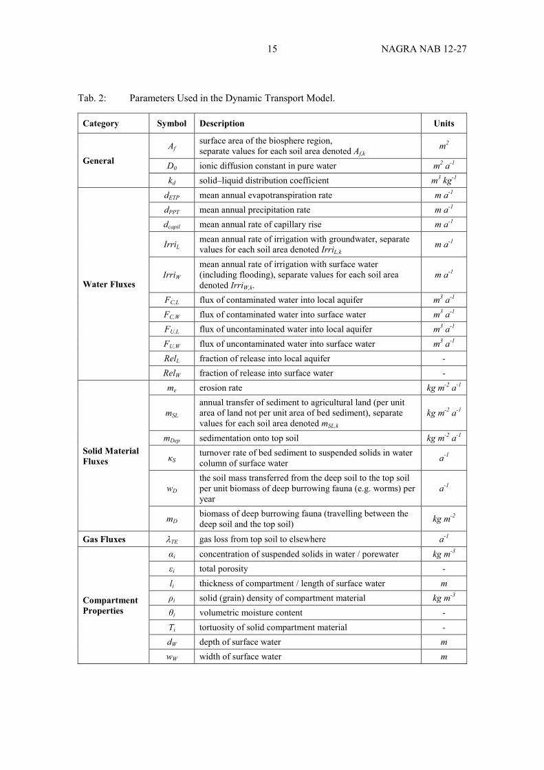
Tab. 2: Parameters Used in the Dynamic Transport Model. ............................................... 15

Tab. 3: Nomenclature of Water Fluxes. .............................................................................. 18

Tab. 4: Nomenclature of Solid Material Fluxes. ................................................................. 21

Tab. 5: Parameters Used in the Exposure Model (in alphabetical order). .......................... 24 List of Figures Fig. 1: Conceptualisation of the Principal Water Fluxes in the Biosphere. ......................... 6

Fig. 2: Conceptualisation of the Principal Solid Material Fluxes in the Biosphere. ............ 7

Fig. 3: Structure of the Compartment Model of the Biosphere. ........................................... 8

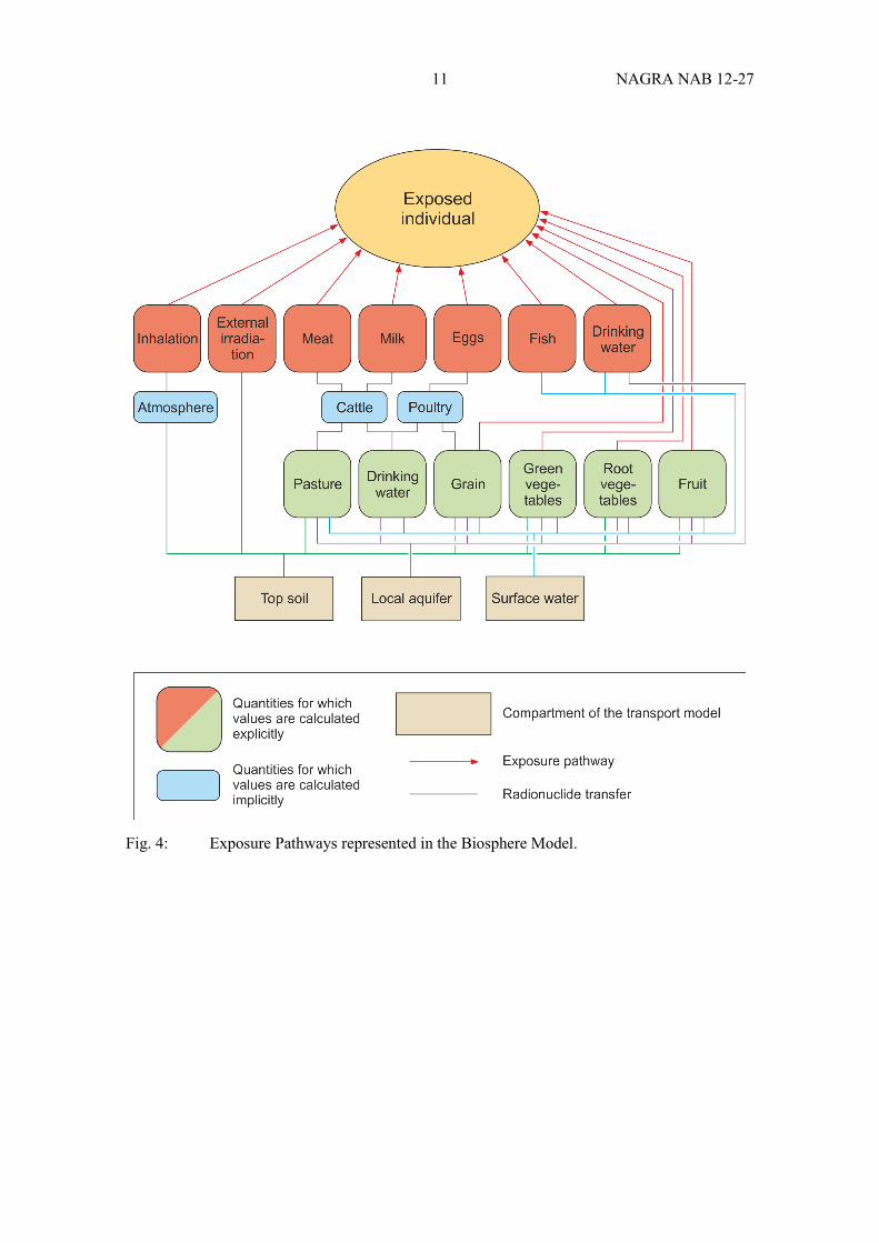
Fig. 4: Exposure Pathways represented in the Biosphere Model. ...................................... 11

Fig. 5: Intercompartmental Water Fluxes. ......................................................................... 17

Fig. 6: Intercompartmental Solid Material Fluxes ............................................................. 19

Fig. 7: Intercompartmental Diffusive Fluxes. .................................................................... 22

1 NAGRA NAB 12-27

1 Introduction Nagra is responsible for the management and disposal of radioactive waste arising in Switzer-land in a way that ensures the long-term protection of man and the environment. The Swiss radioactive waste management program foresees deep geological disposal in two types of facility, one facility for high-level radioactive waste (HLW repository) and one for low- and intermediate-level radioactive waste (L/ILW repository). Nagra requires the capability to assess potential radiological exposures in the biosphere for comparison against regulatory protection criteria, should radionuclides be released from the barrier system of a deep geological repository and migrate to the surface environment over long periods of time after repository closure.

This report documents the conceptual and mathematical basis for Nagra's biosphere assessment model. The model is implemented in a software application and is referred to as the Swiss Biosphere Assessment Code, SwiBAC.

The biosphere model described herein builds on Nagra's previous biosphere model, which was called the Terrestrial-Aquatic Model of the Environment (TAME). Hence, the report draws together a description of the conceptual and mathematical basis for the biosphere model based on NTB 93-04 (Klos et al. 1996), Nagra (2003), NTB 02-06 (Nagra 2002), NAB 08-01 (Brennwald & van Dorp 2008) and NAB 10-15 (Nagra 2010)1. Note that the earlier model has been slightly extended to allow for several agricultural soil areas within the region of interest and to permit additional losses from soil, for example, by volatilization.

Some background is presented in Section 2. The conceptual model is presented in Section 3 and the mathematical model is given in Section 4.

1 Further discussion of the conceptual and mathematical basis can be found in the original documents.

3 NAGRA NAB 12-27

2 Background The development of TAME began with a preliminary analysis of the surface conditions expected in the regions under consideration for deep geological disposal of radioactive waste in Switzerland over the time periods of concern. As a result, inland biospheres with a range of river types from small rivers in tributary valleys to large rivers, such as the Rhine, were identi-fied. Additionally, lakes could potentially form part of such biospheres. Marine and coastal environments were, however, ruled out.

Radionuclide release from deep geological repositories to the biosphere is expected to occur very slowly, if compared to the time scales of human activities, with discharge of deep ground-water to the surface environment. Other release types are possible, but these generally involve disturbances to the normal evolution of the repository system, which are not addressed with the biosphere modelling approach described in this report.

This naturally leads to the division of the biosphere model in two parts: (i) the dynamic modelling of features, events and processes (FEPs) with characteristic timescales greater than years – mainly the physical transport processes between different compartments of the bio-sphere (soils, aquifers as well as surface water bodies), and (ii) the static modelling of FEPs that are related to crops, livestock and humans and the processes that are largely determined by the annual cycle (using an equilibrium approach).

Radiological exposures are evaluated for an average individual within the population group most affected ("critical group"). This group should have habits that are realistic based on a present-day perspective (see ENSI 2009). For the critical group, a self-sustaining agricultural system is considered. This is believed to maximize the exposures of individuals by limiting any significant dilution with external material as well as by preventing losses from the system, except those identified in the dynamic transport model.

The spatial extent of the modelled biosphere depends on the size of the region potentially affected by release from the repository and / or by the minimum area for which the criteria defining the critical group are valid.

5 NAGRA NAB 12-27

3 Conceptual Model

3.1 Features, Events and Processes for Transport in the Biosphere The principal components of a generic, agricultural biosphere system as described in Section 2 are (see Figs. 1 and 2):

• near-surface aquifer;

• surface water (with suspended sediments and bed sediments);

• rooting zone soils;

• lower soil horizons.

These components are associated with one or several compartments, for which homogenous concentrations are postulated.

In modelling the transport of radionuclides between compartments, it is important to recognise that transport can take place in solution (Fig. 1) and with the fluxes of solid materials (Fig. 2). It is therefore important to distinguish between radionuclides in solution and those associated with solid materials. Given that environmental concentrations will be at trace levels, it is possible to model the partitioning between solution and solid materials with an equilibrium approach (Kd concept).

Diffusion in the aqueous phase between compartments of varying concentrations may also play a role, provided its contribution is not out-weighed by advective / dispersive transport and provided the mathematical formulation of diffusive transport does not conflict with the assump-tion of homogenous concentrations within the compartments and with the lower limit for time-scales of interest (the annual cycle). As a result, only vertical diffusion processes between the near-surface aquifer and the soil compartments are considered.

Some radionuclides may also enter the gas phase in the biosphere. Nagra (2013) shows that the biosphere model should include the possibility for C-14 to be released from the rooting zone soil solution to the soil gas phase, and to be potentially lost from the biosphere via the gas phase. The inclusion of an additional loss term from the rooting zone soil allows these processes to be included for C-14 and for other radionuclides, for which a loss in the gas phase may be important, such as Se-79 (e.g. Smith et al. 2009).2

The model assumes that the rooting zone soil is well mixed on relatively small timescales (if compared to radionuclide release rates from the geological barrier) and that the near-surface aquifer can be treated as a homogenous unit. Similarly, the intermediate soil horizons between the aquifer and the rooting zone are treated as a single entity. In the aquatic environment a distinction is made between the surface water and bed sediments.

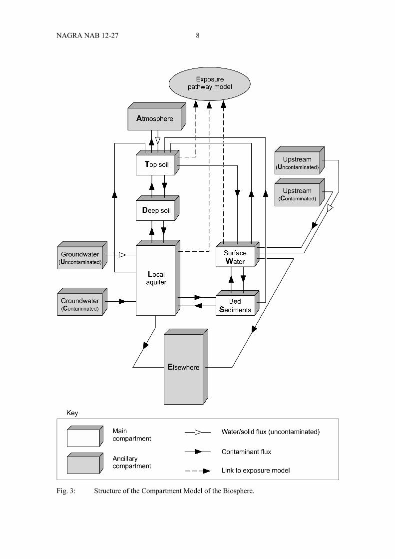
In total, five main types of compartment (rooting zone soil, near-surface aquifer, lower soil hori-zons, surface water and bed sediments) together with some ancillary compartments are con-sidered for modelling the transport of radionuclides within the biosphere. These are shown in Fig. 3. The names of the compartments have distinct meanings and they are used in the mathe-matical representation to identify compartments and transfer between compartments; Table 1 summarises the respective nomenclature.

2 As discussed in Nagra (2013), such loss terms alter the original assessment strategy and require the adaption of the interface between the sub-models for radionuclide transport and for human exposure due to radionuclide concentrations in the environment.

NAGRA NAB 12-27 6

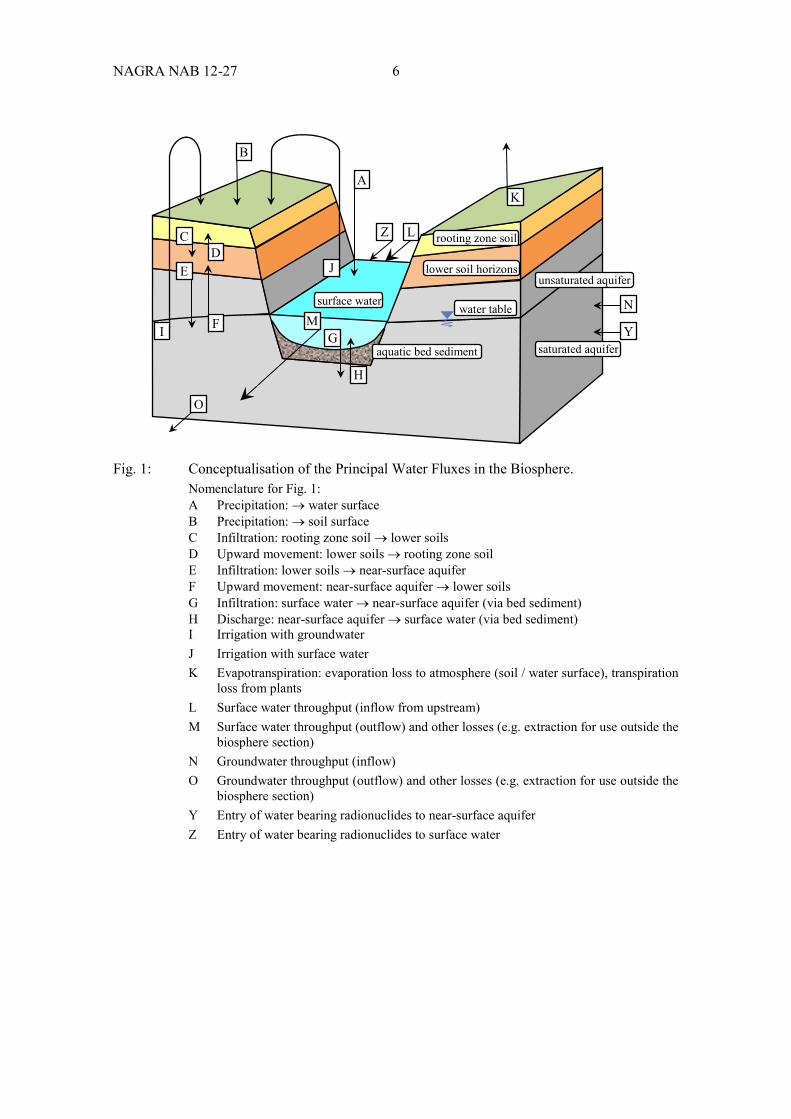
Fig. 1: Conceptualisation of the Principal Water Fluxes in the Biosphere. Nomenclature for Fig. 1: A Precipitation: → water surface B Precipitation: → soil surface C Infiltration: rooting zone soil → lower soils D Upward movement: lower soils → rooting zone soil E Infiltration: lower soils → near-surface aquifer F Upward movement: near-surface aquifer → lower soils G Infiltration: surface water → near-surface aquifer (via bed sediment) H Discharge: near-surface aquifer → surface water (via bed sediment) I Irrigation with groundwater J Irrigation with surface water K Evapotranspiration: evaporation loss to atmosphere (soil / water surface), transpiration

loss from plants L Surface water throughput (inflow from upstream) M Surface water throughput (outflow) and other losses (e.g. extraction for use outside the

biosphere section) N Groundwater throughput (inflow) O Groundwater throughput (outflow) and other losses (e.g. extraction for use outside the

biosphere section) Y Entry of water bearing radionuclides to near-surface aquifer Z Entry of water bearing radionuclides to surface water

surface water

rooting zone soil

lower soil horizons unsaturated aquifer

saturated aquifer

water table

A

B

C D

E

F G

H

I

J

K

L

M N

O

Y

Z

aquatic bed sediment

7 NAGRA NAB 12-27

Fig. 2: Conceptualisation of the Principal Solid Material Fluxes in the Biosphere. Nomenclature for Fig. 2: a External deposition on surface water (e.g. from erosion elsewhere) b External deposition on soil surface (e.g. from erosion elsewhere) c Bioturbation and water-mediated transport: rooting zone soil → lower soils d Bioturbation: lower soils → rooting zone soil i Solid material in irrigation water from the aquifer j Flooding, dredging and irrigation: suspended solid material and bed sediment

→ soils (rooting zone) l Suspended sediment throughput (inflow) m Suspended sediment throughput (outflow) p Erosion: rooting zone soil → surface water q Deposition: waterborne solid material → bed sediment r Resuspension: aquatic bed sediments → surface water

The compartmentalisation in Fig. 3 implies that, e.g. the same irrigation or erosion regime applies to the entire area. In order to allow for different regimes within the area, the soil compartments (top and deep soil) can be split into several separate smaller areas. Each such smaller area may then have different soil properties or irrigation regimes.

surface water

rooting zone soil

lower soil horizons unsaturated aquifer

saturated aquifer

water table

a

b

c d

q r

i

j

l

m

aquatic bed sediment

p

NAGRA NAB 12-27 8

Fig. 3: Structure of the Compartment Model of the Biosphere.

9 NAGRA NAB 12-27

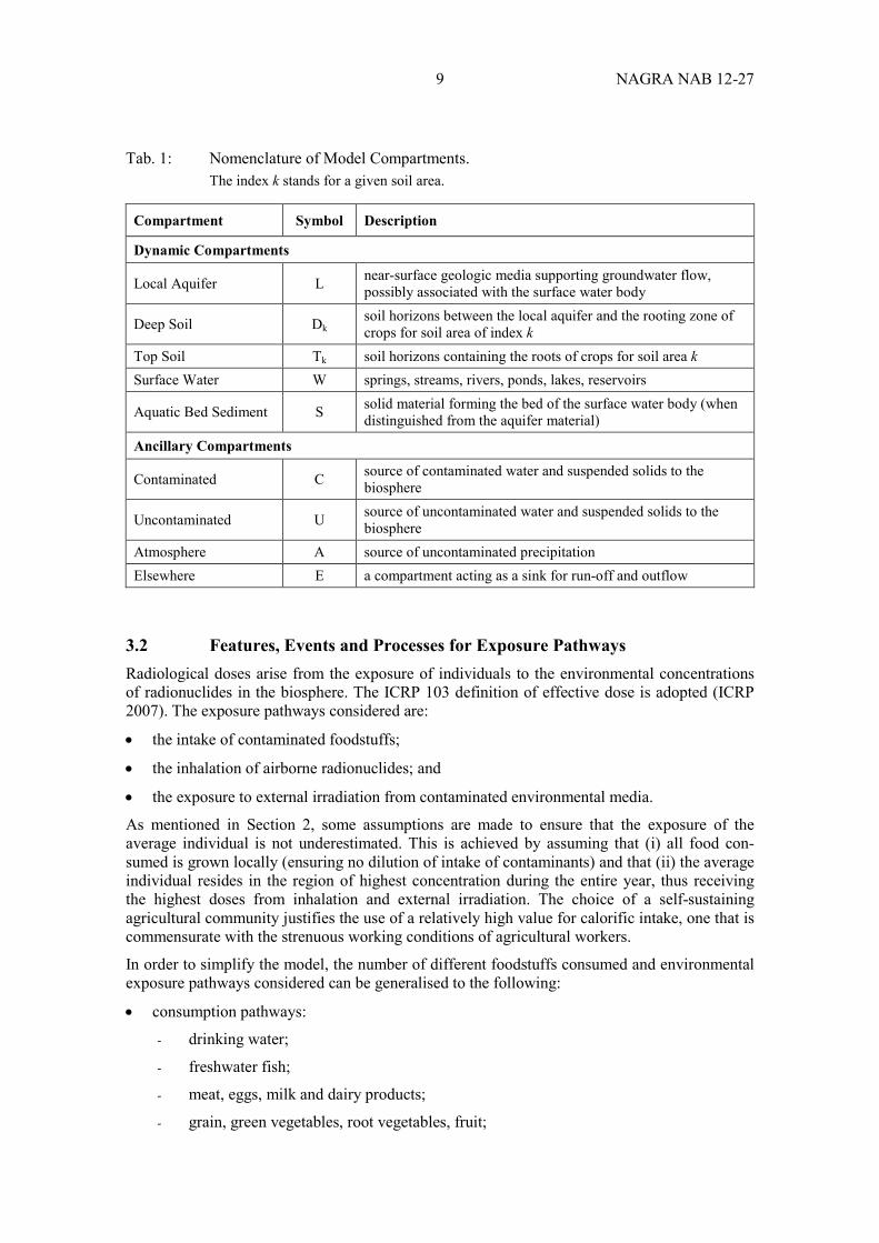
Tab. 1: Nomenclature of Model Compartments. The index k stands for a given soil area.

Compartment Symbol Description

Dynamic Compartments

Local Aquifer L near-surface geologic media supporting groundwater flow, possibly associated with the surface water body

Deep Soil Dk soil horizons between the local aquifer and the rooting zone of crops for soil area of index k

Top Soil Tk soil horizons containing the roots of crops for soil area k Surface Water W springs, streams, rivers, ponds, lakes, reservoirs

Aquatic Bed Sediment S solid material forming the bed of the surface water body (when distinguished from the aquifer material)

Ancillary Compartments

Contaminated C source of contaminated water and suspended solids to the biosphere

Uncontaminated U source of uncontaminated water and suspended solids to the biosphere

Atmosphere A source of uncontaminated precipitation Elsewhere E a compartment acting as a sink for run-off and outflow

3.2 Features, Events and Processes for Exposure Pathways Radiological doses arise from the exposure of individuals to the environmental concentrations of radionuclides in the biosphere. The ICRP 103 definition of effective dose is adopted (ICRP 2007). The exposure pathways considered are:

• the intake of contaminated foodstuffs;

• the inhalation of airborne radionuclides; and

• the exposure to external irradiation from contaminated environmental media.

As mentioned in Section 2, some assumptions are made to ensure that the exposure of the average individual is not underestimated. This is achieved by assuming that (i) all food con-sumed is grown locally (ensuring no dilution of intake of contaminants) and that (ii) the average individual resides in the region of highest concentration during the entire year, thus receiving the highest doses from inhalation and external irradiation. The choice of a self-sustaining agricultural community justifies the use of a relatively high value for calorific intake, one that is commensurate with the strenuous working conditions of agricultural workers.

In order to simplify the model, the number of different foodstuffs consumed and environmental exposure pathways considered can be generalised to the following:

• consumption pathways:

- drinking water;

- freshwater fish;

- meat, eggs, milk and dairy products;

- grain, green vegetables, root vegetables, fruit;

NAGRA NAB 12-27 10

• environmental exposures:

- external irradiation;

- inhalation of radioactive dust or radioactive gas having escaped from the rooting zone.

One further reason for this generalisation is that the database for food consumption is sparse and often contradictory. Best-estimate parameters for a small number of generic consumption pathways are therefore more reliable. For an agricultural lifestyle, limited time would be spent close to the water bodies, so inhalation of gas and aerosols from surface water is neglected.

All radionuclides removed from the biosphere compartments by the action of radiation exposure are assumed to be recycled annually so that the exposures are not diminished by the pathways acting as external sinks to the transport model.

Fig. 4 shows the network of exposure pathways considered. Radionuclide concentrations in crops and other vegetation arise from:

• root uptake;

• irrigation and foliar absorption; and

• soil particles on external surfaces.

Similarly, concentrations of contaminants in animal tissues and other products arise from:

• drinking water consumption;

• intake of contaminated foodstuffs;

• the direct intake of contaminated soils.

Only external irradiation and drinking water pathways (from the local aquifer or from the sur-face water compartment) are directly connected to radionuclide concentrations in the biosphere. The other exposure pathways take account of intermediate FEPs, as illustrated in Fig. 4.

Where multiple soil areas are included, each crop (including pasture) is assumed to be grown in a particular area and so the relevant top soil compartment is used. External irradiation and dust inhalation are treated by averaging (weighted by area) over all the top soil areas.

11 NAGRA NAB 12-27

Fig. 4: Exposure Pathways represented in the Biosphere Model.

13 NAGRA NAB 12-27

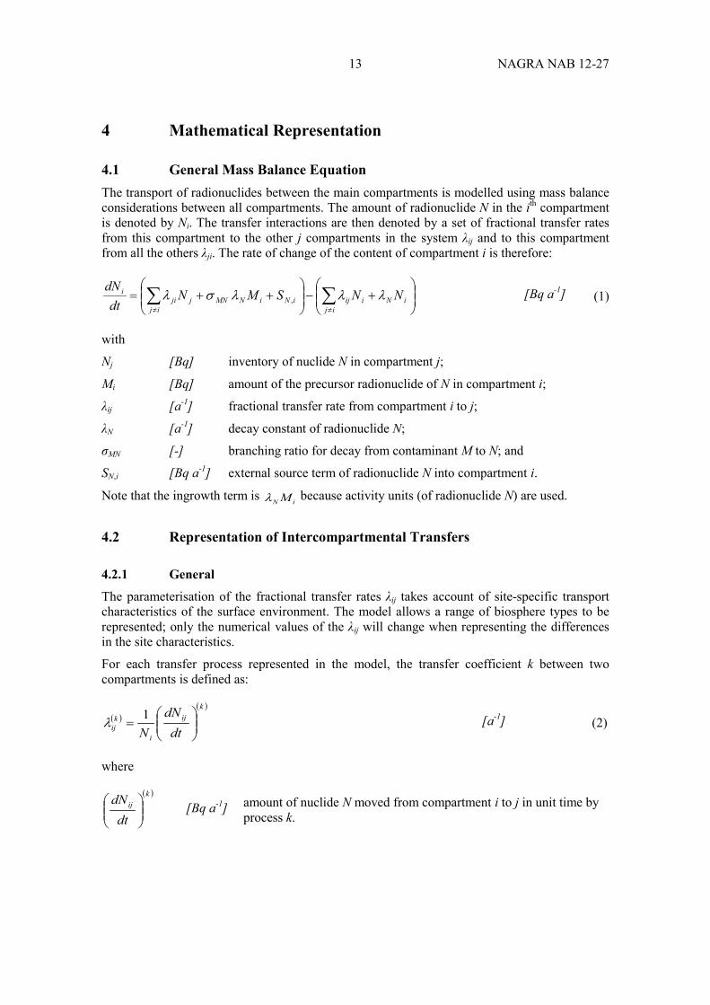
4 Mathematical Representation

4.1 General Mass Balance Equation The transport of radionuclides between the main compartments is modelled using mass balance considerations between all compartments. The amount of radionuclide N in the ith compartment is denoted by Ni. The transfer interactions are then denoted by a set of fractional transfer rates from this compartment to the other j compartments in the system λij and to this compartment from all the others λji. The rate of change of the content of compartment i is therefore:

+−

++= ∑∑

≠≠ ijiNiij

ijiNiNMNjji

i NNSMNdt

dNλλλσλ , [Bq a-1] (1)

with

Nj [Bq] inventory of nuclide N in compartment j;

Mi [Bq] amount of the precursor radionuclide of N in compartment i;

λij [a-1] fractional transfer rate from compartment i to j;

λN [a-1] decay constant of radionuclide N;

σMN [-] branching ratio for decay from contaminant M to N; and

SN,i [Bq a-1] external source term of radionuclide N into compartment i.

Note that the ingrowth term is iN Mλ because activity units (of radionuclide N) are used.

4.2 Representation of Intercompartmental Transfers

4.2.1 General

The parameterisation of the fractional transfer rates λij takes account of site-specific transport characteristics of the surface environment. The model allows a range of biosphere types to be represented; only the numerical values of the λij will change when representing the differences in the site characteristics.

For each transfer process represented in the model, the transfer coefficient k between two compartments is defined as:

( )( )k

ij

i

kij dt

dNN

=

1λ [a-1] (2)

where

( )kij

dtdN

[Bq a-1] amount of nuclide N moved from compartment i to j in unit time by process k.

NAGRA NAB 12-27 14

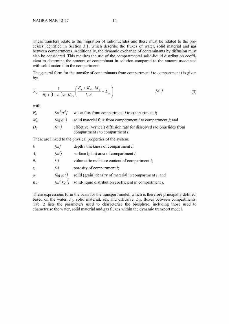
These transfers relate to the migration of radionuclides and these must be related to the pro-cesses identified in Section 3.1, which describe the fluxes of water, solid material and gas between compartments. Additionally, the dynamic exchange of contaminants by diffusion must also be considered. This requires the use of the compartmental solid-liquid distribution coeffi-cient to determine the amount of contaminant in solution compared to the amount associated with solid material in the compartment.

The general form for the transfer of contaminants from compartment i to compartment j is given by:

( )

+

+

−+= ij

ii

ijidij

idiiiij D

AlMKF

K,

,11

ρεθλ [a-1] (3)

with

Fij [m3 a-1] water flux from compartment i to compartment j;

Mij [kg a-1] solid material flux from compartment i to compartment j; and

Dij [a-1] effective (vertical) diffusion rate for dissolved radionuclides from compartment i to compartment j.

These are linked to the physical properties of the system:

li [m] depth / thickness of compartment i;

Ai [m2] surface (plan) area of compartment i;

θi [-] volumetric moisture content of compartment i;

εi [-] porosity of compartment i;

ρi [kg m-3] solid (grain) density of material in compartment i; and

Kd,i [m3 kg-1] solid-liquid distribution coefficient in compartment i.

These expressions form the basis for the transport model, which is therefore principally defined, based on the water, Fij, solid material, Mij, and diffusive, Dij, fluxes between compartments. Tab. 2 lists the parameters used to characterise the biosphere, including those used to characterise the water, solid material and gas fluxes within the dynamic transport model.

15 NAGRA NAB 12-27

Tab. 2: Parameters Used in the Dynamic Transport Model.

Category Symbol Description Units

General Af

surface area of the biosphere region, separate values for each soil area denoted Af,k

m2

D0 ionic diffusion constant in pure water m2 a-1

kd solid–liquid distribution coefficient m3 kg-1

Water Fluxes

dETP mean annual evapotranspiration rate m a-1

dPPT mean annual precipitation rate m a-1

dcapil mean annual rate of capillary rise m a-1

IrriL mean annual rate of irrigation with groundwater, separate values for each soil area denoted IrriL,k

m a-1

IrriW

mean annual rate of irrigation with surface water (including flooding), separate values for each soil area denoted IrriW,k.

m a-1

FC,L flux of contaminated water into local aquifer m3 a-1 FC,W flux of contaminated water into surface water m3 a-1 FU,L flux of uncontaminated water into local aquifer m3 a-1 FU,W flux of uncontaminated water into surface water m3 a-1 RelL fraction of release into local aquifer - RelW fraction of release into surface water -

Solid Material Fluxes

me erosion rate kg m-2 a-1

mSL

annual transfer of sediment to agricultural land (per unit area of land not per unit area of bed sediment), separate values for each soil area denoted mSL,k

kg m-2 a-1

mDep sedimentation onto top soil kg m-2 a-1

κS turnover rate of bed sediment to suspended solids in water column of surface water a-1

wD

the soil mass transferred from the deep soil to the top soil per unit biomass of deep burrowing fauna (e.g. worms) per year

a-1

mD biomass of deep burrowing fauna (travelling between the deep soil and the top soil) kg m-2

Gas Fluxes λTE gas loss from top soil to elsewhere a-1

Compartment Properties

αi concentration of suspended solids in water / porewater kg m-3 εi total porosity - li thickness of compartment / length of surface water m ρi solid (grain) density of compartment material kg m-3 θi volumetric moisture content - Ti tortuosity of solid compartment material - dW depth of surface water m wW width of surface water m

NAGRA NAB 12-27 16

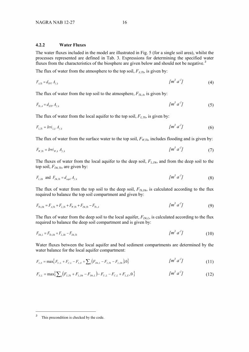
4.2.2 Water Fluxes

The water fluxes included in the model are illustrated in Fig. 5 (for a single soil area), whilst the processes represented are defined in Tab. 3. Expressions for determining the specified water fluxes from the characteristics of the biosphere are given below and should not be negative.3

The flux of water from the atmosphere to the top soil, FA,Tk, is given by:

kfPPTTkA AdF ,, = [m3 a-1] (4)

The flux of water from the top soil to the atmosphere, FTk,A, is given by:

kfETPATk AdF ,, = [m3 a-1] (5)

The flux of water from the local aquifer to the top soil, FL,Tk, is given by:

kfkLTkL AIrriF ,,, = [m3 a-1] (6)

The flux of water from the surface water to the top soil, FW,Tk, includes flooding and is given by:

kfkWTkW AIrriF ,,, = [m3 a-1] (7)

The fluxes of water from the local aquifer to the deep soil, FL,Dk, and from the deep soil to the top soil, FDk,Tk, are given by:

kfcapilTkDkDkL AdFF ,,, and = [m3 a-1] (8)

The flux of water from the top soil to the deep soil, FTk,Dk, is calculated according to the flux required to balance the top soil compartment and given by:

ATkTkDkTkWTkLTkADkTk FFFFFF ,,,,,, −+++= [m3 a-1] (9)

The flux of water from the deep soil to the local aquifer, FDk,L, is calculated according to the flux required to balance the deep soil compartment and is given by:

TkDkDkLDkTkLDk FFFF ,,,, −+= [m3 a-1] (10)

Water fluxes between the local aquifer and bed sediment compartments are determined by the water balance for the local aquifer compartment:

( ){ }0,max ,,,,,,, ∑ −−+−+=k DkLTkLLDkELLCLUSL FFFFFFF [m3 a-1] (11)

( ){ }0,max ,,,,,,, ELLCLUk LDkDkLTkLLS FFFFFFF +−−−+= ∑ [m3 a-1] (12)

3 This precondition is checked by the code.

17 NAGRA NAB 12-27

Similarly, water fluxes between the bed sediment and the surface water are determined by the water balance for the bed sediment compartment:

{ }0max ,FFF L,SS,LW,S −= [m3 a-1] (13)

{ }0max ,FFF S,LL,SS,W −= [m3 a-1] (14)

The water flux from the surface water to elsewhere is given by:

∑−−++=k TkWSWWSWCWUEW FFFFFF ,,,,,, [m3 a-1] (15)

Explicitly specified Calculated through water balance

Key to arrows:

Top Soil T

Deep Soil D

Local Aquifer L

Surface Water W

Bed Sediment S

Elsewhere E

FTA FAT

FDT FTD

FLD FDL

FLT

FUL FCL

FSL

FLS

FSW FWS

FWT

FWE

FUW FCW

FLE

Fig. 5: Intercompartmental Water Fluxes. Situation for a model with a single soil area.

NAGRA NAB 12-27 18

Tab. 3: Nomenclature of Water Fluxes. Water fluxes are volumetric, [m3 a-1].

Symbol Description

FA,Tk precipitation for soil area k FTk,A evapotranspiration for soil area k FL,Tk irrigation with groundwater (from local aquifer) for soil area k FW,Tk flooding and irrigation with surface water for soil area k FTk,Dk percolation from top soil to deep soil for soil area k FDk,Tk water flux from deep soil to top soil (e.g. capillary rise) for soil area k FDk,L percolation from deep soil to local aquifer for soil area k FL,Dk water flux from local aquifer to deep soil (e.g. capillary rise) for soil area k FU,L flux of uncontaminated groundwater into local aquifer FC,L discharge of contaminated groundwater into local aquifer FL,S water flux from local aquifer to bed sediments FS,L water flux from bed sediments to local aquifer FS,W water flux from bed sediments to surface water FW,S water flux from surface water to bed sediments

FU,W flux of uncontaminated water into surface water (mainly from upstream surface water , but also precipitation)

FC,W flux of contaminated water into surface water FW,E water flux from surface water to sink (out of the model area) FL,E water flux from local aquifer to sink (out of the model area)

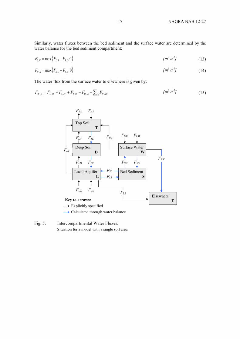
4.2.3 Solid Material Fluxes

The solid material fluxes included in the model are illustrated in Fig. 6, whilst the processes represented are defined in Tab. 4. Expressions for determining the specified fluxes of solid material from the characteristics of the biosphere are given below and should not be negative.

Water fluxes between compartments may carry suspended sediment, which is included in the solid material balance model according to:

jiisusp

ji FM ,, α= [kg a-1] (16)

The transfer of suspended solids is the only way by which solid material is transferred between the following compartments:

• uncontaminated water to surface water, MU,W, in which case the suspended sediment concentration in the surface water is used, αW;

• local aquifer to the top soil, ML,Tk;

• surface water to top soil, MW,Tk;

• local aquifer to bed sediments, ML,S;

• bed sediments to local aquifer, MS,L.

19 NAGRA NAB 12-27

MST

Top Soil T

Deep Soil D

Local Aquifer L

Surface Water W

Bed Sediment S

Elsewhere E

MDT MTD

MLD MDL

MLT

MUL MCL

MSL

MLS

MSW MWS

MWT

MWE

MUW

MTW

Explicitly specified Calculated through mass balance

Key to arrows:

Includes explicitly specified contribution (bioturbation) and mass balance

MLE

MUT

Fig. 6: Intercompartmental Solid Material Fluxes. Situation for a model with a single soil area.

The solid material flux from top soil to surface water as a result of erosion, erosionWTkM , , is given

by:

kfeerosion

WTk AmM ,, = [kg a-1] (17)

The flux of uncontaminated solid material to the top soil due to deposition (e.g. after flooding), deposition

TkUM , , is given by:

kfDepdeposition

TkU AmM ,, = [kg a-1] (18)

The flux of solid material from bed sediment to top soil due to dredging practices is given by:

kfkSLdredging

TkS AmM ,,, = [kg a-1] (19)

NAGRA NAB 12-27 20

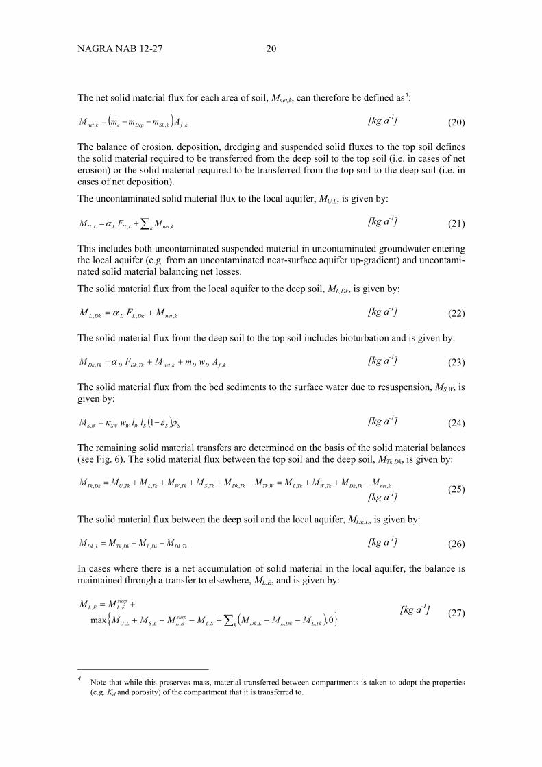
The net solid material flux for each area of soil, Mnet,k, can therefore be defined as4:

( ) kfkSLDepeknet AmmmM ,,, −−= [kg a-1] (20)

The balance of erosion, deposition, dredging and suspended solid fluxes to the top soil defines the solid material required to be transferred from the deep soil to the top soil (i.e. in cases of net erosion) or the solid material required to be transferred from the top soil to the deep soil (i.e. in cases of net deposition).

The uncontaminated solid material flux to the local aquifer, MU,L, is given by:

∑+=k knetLULLU MFM ,,, α [kg a-1] (21)

This includes both uncontaminated suspended material in uncontaminated groundwater entering the local aquifer (e.g. from an uncontaminated near-surface aquifer up-gradient) and uncontami-nated solid material balancing net losses.

The solid material flux from the local aquifer to the deep soil, ML,Dk, is given by:

knetDkLLDkL MFM ,,, += α [kg a-1] (22)

The solid material flux from the deep soil to the top soil includes bioturbation and is given by:

kfDDknetTkDkDTkDk AwmMFM ,,,, ++=α [kg a-1] (23)

The solid material flux from the bed sediments to the surface water due to resuspension, MS,W, is given by:

( ) SSSWWSWWS llwM ρεκ −= 1, [kg a-1] (24)

The remaining solid material transfers are determined on the basis of the solid material balances (see Fig. 6). The solid material flux between the top soil and the deep soil, MTk,Dk, is given by:

knetTkDkTkWTkLWTkTkDkTkSTkWTkLTkUDkTk MMMMMMMMMMM ,,,,,,,,,,, −++=−++++= [kg a-1]

(25)

The solid material flux between the deep soil and the local aquifer, MDk,L, is given by:

TkDkDkLDkTkLDk MMMM ,,,, −+= [kg a-1] (26)

In cases where there is a net accumulation of solid material in the local aquifer, the balance is maintained through a transfer to elsewhere, ML,E, and is given by:

( ){ }0max ,MMMMMMM

MM

k Tk,LDk,LL,DkS,Lsusp

E,LL,SL,U

suspE,LE,L

∑ −−+−−+

+= [kg a-1] (27)

4 Note that while this preserves mass, material transferred between compartments is taken to adopt the properties (e.g. Kd and porosity) of the compartment that it is transferred to.

21 NAGRA NAB 12-27

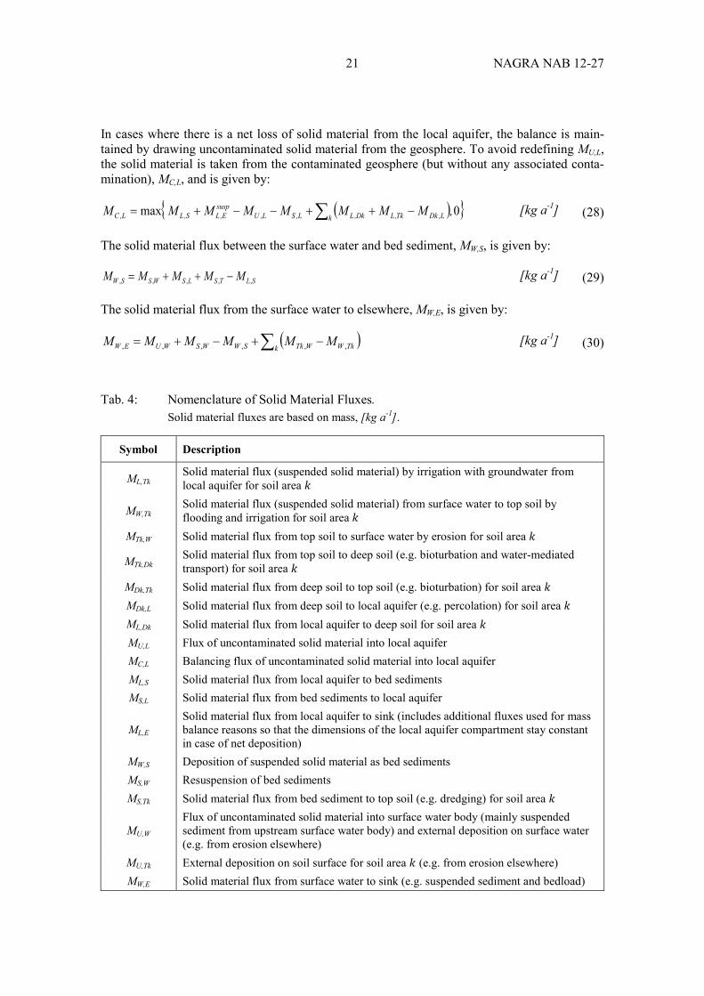
In cases where there is a net loss of solid material from the local aquifer, the balance is main-tained by drawing uncontaminated solid material from the geosphere. To avoid redefining MU,L, the solid material is taken from the contaminated geosphere (but without any associated conta-mination), MC,L, and is given by:

( ){ }0max ,MMMMMMMMk L,DkTk,LDk,LL,SL,U

suspE,LS,LL,C ∑ −++−−+= [kg a-1] (28)

The solid material flux between the surface water and bed sediment, MW,S, is given by:

SLTSLSWSSW MMMMM ,,,,, −++= [kg a-1] (29)

The solid material flux from the surface water to elsewhere, MW,E, is given by:

( )∑ −+−+=k TkWWTkSWWSWUEW MMMMMM ,,,,,, [kg a-1] (30)

Tab. 4: Nomenclature of Solid Material Fluxes. Solid material fluxes are based on mass, [kg a-1].

Symbol Description

ML,Tk Solid material flux (suspended solid material) by irrigation with groundwater from local aquifer for soil area 𝑘𝑘

MW,Tk Solid material flux (suspended solid material) from surface water to top soil by flooding and irrigation for soil area 𝑘𝑘

MTk,W Solid material flux from top soil to surface water by erosion for soil area 𝑘𝑘

MTk,Dk Solid material flux from top soil to deep soil (e.g. bioturbation and water-mediated transport) for soil area 𝑘𝑘

MDk,Tk Solid material flux from deep soil to top soil (e.g. bioturbation) for soil area 𝑘𝑘 MDk,L Solid material flux from deep soil to local aquifer (e.g. percolation) for soil area 𝑘𝑘 ML,Dk Solid material flux from local aquifer to deep soil for soil area 𝑘𝑘 MU,L Flux of uncontaminated solid material into local aquifer MC,L Balancing flux of uncontaminated solid material into local aquifer ML,S Solid material flux from local aquifer to bed sediments MS,L Solid material flux from bed sediments to local aquifer

ML,E

Solid material flux from local aquifer to sink (includes additional fluxes used for mass balance reasons so that the dimensions of the local aquifer compartment stay constant in case of net deposition)

MW,S Deposition of suspended solid material as bed sediments MS,W Resuspension of bed sediments MS,Tk Solid material flux from bed sediment to top soil (e.g. dredging) for soil area 𝑘𝑘

MU,W Flux of uncontaminated solid material into surface water body (mainly suspended sediment from upstream surface water body) and external deposition on surface water (e.g. from erosion elsewhere)

MU,Tk External deposition on soil surface for soil area 𝑘𝑘 (e.g. from erosion elsewhere) MW,E Solid material flux from surface water to sink (e.g. suspended sediment and bedload)

NAGRA NAB 12-27 22

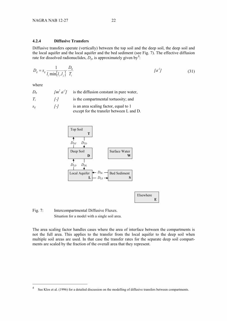
4.2.4 Diffusive Transfers

Diffusive transfers operate (vertically) between the top soil and the deep soil, the deep soil and the local aquifer and the local aquifer and the bed sediment (see Fig. 7). The effective diffusion rate for dissolved radionuclides, Dij, is approximately given by5:

{ } ijiiijij T

Dl,ll

sD 0

min1

⋅= [a-1] (31)

where

D0 [m2 a-1] is the diffusion constant in pure water,

Ti [-] is the compartmental tortuosity; and

sij [-] is an area scaling factor, equal to 1 except for the transfer between L and D.

Top Soil T

Deep Soil D

Local Aquifer L

Surface Water W

Bed Sediment S

Elsewhere E

DDT DTD

DLD DDL

DSL

DLS

Fig. 7: Intercompartmental Diffusive Fluxes. Situation for a model with a single soil area.

The area scaling factor handles cases where the area of interface between the compartments is not the full area. This applies to the transfer from the local aquifer to the deep soil when multiple soil areas are used. In that case the transfer rates for the separate deep soil compart-ments are scaled by the fraction of the overall area that they represent.

5 See Klos et al. (1996) for a detailed discussion on the modelling of diffusive transfers between compartments.

23 NAGRA NAB 12-27

4.2.5 Gas Transfers

The gas loss transfer from the top soil is represented as a specified transfer rate, λTE, to outside the biosphere system. This is illustrated conceptually in Fig. 3 as a transfer to the atmosphere. The transfer takes radionuclides out of the biosphere system via the atmosphere and so it is represented in the model as a transfer to elsewhere. If the gas loss contributes to inhalation exposures, then the gas loss rate can also be used in the exposure model, see Section 4.3.9.

4.3 Representation of Exposure Pathways The dynamic transport model provides time-dependent inventories of radionuclide N in compartment i as a function of time, Ni(t). The annual individual effective dose from exposure to radionuclide N in all compartments i for exposure pathway p, ( ) ( )tD N

p , is given by:

( ) ( ) ( ) ( )∑=i

iippNN

p tNPEHtD ,exp

[Sv a-1] (32)

with

( )NpD [Sv a-1] annual individual effective dose from exposure to radionuclide N in

each of the i compartments for exposure pathway p

Ni [Bq] time-dependent inventory of N in compartment i

Pp,i

[Ep Pp,i] = a-1

a processing factor that converts the inventory in compartment i, Ni, into a concentration;

Ep an exposure factor for the pathway, e.g. consumption rate or occupancy; and

( )NH exp [Sv Bq-1] the dose per unit intake or exposure for radionuclide N.

Tab. 5 lists the parameters used in the exposure model together with the location of the para-meter values.

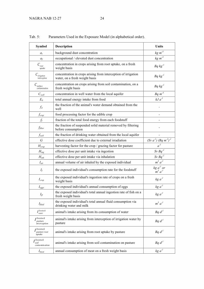
NAGRA NAB 12-27 24

Tab. 5: Parameters Used in the Exposure Model (in alphabetical order).

Symbol Description Units

ar background dust concentration kg m-3

af occupational / elevated dust concentration kg m-3

uptakerootC concentration in crops arising from root uptake, on a fresh

weight basis Bq kg-1

onintercepti irrigationC concentration in crops arising from interception of irrigation

water, on a fresh weight basis Bq kg-1

ioncontaminat surfaceC concentration on crops arising from soil contamination, on a

fresh weight basis Bq kg-1

Cwell concentration in well water from the local aquifer Bq m-3

E0 total annual energy intake from food kJ a-1

fA the fraction of the animal's water demand obtained from the well -

fcrop food processing factor for the edible crop - ff fraction of the total food energy from each foodstuff -

ffilter the fraction of suspended solid material removed by filtering before consumption -

fwell the fraction of drinking water obtained from the local aquifer - G effective dose coefficient due to external irradiation (Sv a-1) (Bq m-3)-1

Hcrop harvesting factor for the crop / grazing factor for pasture a-1

Hing effective dose per unit intake via ingestion Sv Bq-1

Hinh effective dose per unit intake via inhalation Sv Bq-1

Iair annual volume of air inhaled by the exposed individual m3 a-1

If the exposed individual's consumption rate for the foodstuff kg a-1 or m3 a-1

Icrop the exposed individual's ingestion rate of crops on a fresh weight basis kg a-1

Ieggs the exposed individual's annual consumption of eggs kg a-1

Iff the exposed individual's total annual ingestion rate of fish on a fresh weight basis kg a-1

Ifluid the exposed individual's total annual fluid consumption via drinking water and milk m3 a-1

livestockwaterI animal's intake arising from its consumption of water Bq d-1

livestock

erceptionintpastureI animal's intake arising from interception of irrigation water by

pasture Bq d-1

livestock

uptakerootpastureI animal's intake arising from root uptake by pasture Bq d-1

livestock

ationmincontasoilI animal's intake arising from soil contamination on pasture Bq d-1

Imeat annual consumption of meat on a fresh weight basis kg a-1

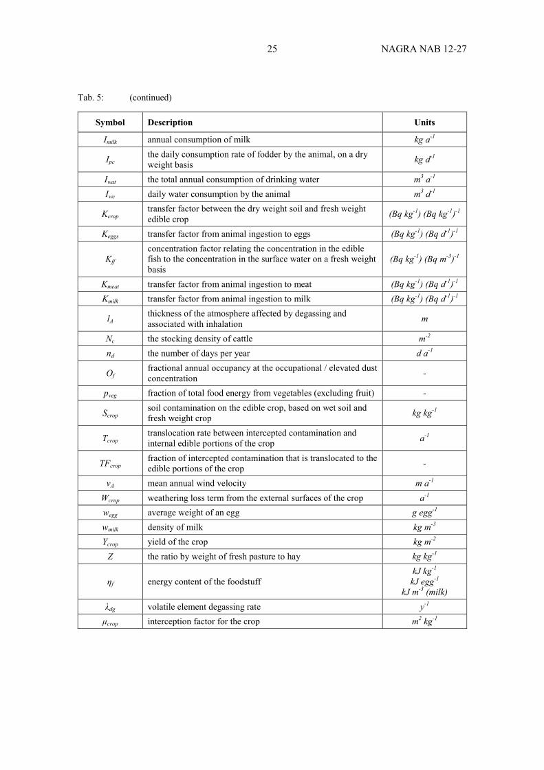
25 NAGRA NAB 12-27

Tab. 5: (continued)

Symbol Description Units

Imilk annual consumption of milk kg a-1

Ipc the daily consumption rate of fodder by the animal, on a dry weight basis kg d-1

Iwat the total annual consumption of drinking water m3 a-1

Iwc daily water consumption by the animal m3 d-1

Kcrop transfer factor between the dry weight soil and fresh weight edible crop (Bq kg-1) (Bq kg-1)-1

Keggs transfer factor from animal ingestion to eggs (Bq kg-1) (Bq d-1)-1

Kff

concentration factor relating the concentration in the edible fish to the concentration in the surface water on a fresh weight basis

(Bq kg-1) (Bq m-3)-1

Kmeat transfer factor from animal ingestion to meat (Bq kg-1) (Bq d-1)-1

Kmilk transfer factor from animal ingestion to milk (Bq kg-1) (Bq d-1)-1

lA thickness of the atmosphere affected by degassing and associated with inhalation m

Nc the stocking density of cattle m-2

nd the number of days per year d a-1

Of fractional annual occupancy at the occupational / elevated dust concentration -

pveg fraction of total food energy from vegetables (excluding fruit) -

Scrop soil contamination on the edible crop, based on wet soil and fresh weight crop kg kg-1

Tcrop translocation rate between intercepted contamination and internal edible portions of the crop a-1

TFcrop fraction of intercepted contamination that is translocated to the edible portions of the crop -

vA mean annual wind velocity m a-1

Wcrop weathering loss term from the external surfaces of the crop a-1

wegg average weight of an egg g egg-1

wmilk density of milk kg m-3

Ycrop yield of the crop kg m-2 Z the ratio by weight of fresh pasture to hay kg kg-1

ηf energy content of the foodstuff kJ kg-1

kJ egg-1

kJ m-3 (milk) λdg volatile element degassing rate y-1

μcrop interception factor for the crop m2 kg-1

NAGRA NAB 12-27 26

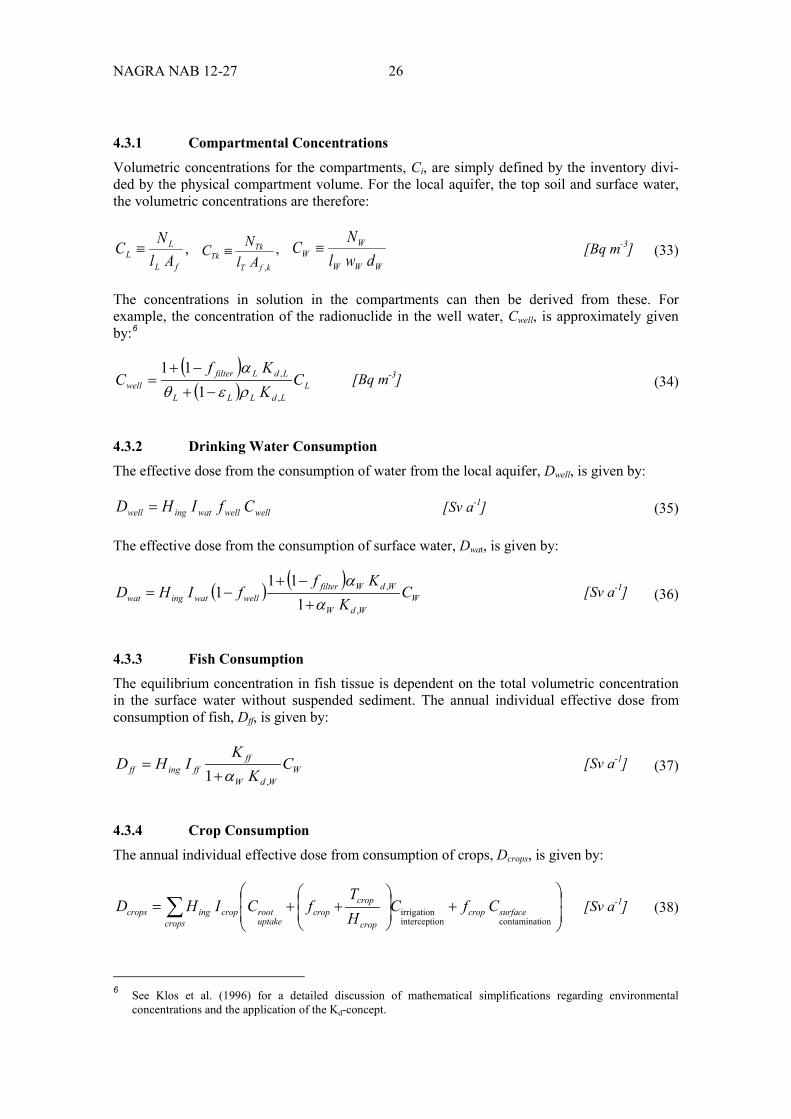
4.3.1 Compartmental Concentrations

Volumetric concentrations for the compartments, Ci, are simply defined by the inventory divi-ded by the physical compartment volume. For the local aquifer, the top soil and surface water, the volumetric concentrations are therefore:

fL

LL Al

NC ≡ , kfT

TkTk Al

NC,

≡ , WWW

WW dwl

NC ≡ [Bq m-3] (33)

The concentrations in solution in the compartments can then be derived from these. For example, the concentration of the radionuclide in the well water, Cwell, is approximately given by:6

( )( ) L

LdLLL

LdLfilterwell C

KKf

C,

,

111

ρεθα

−+

−+= [Bq m-3] (34)

4.3.2 Drinking Water Consumption

The effective dose from the consumption of water from the local aquifer, Dwell, is given by:

wellwellwatingwell CfIHD = [Sv a-1] (35)

The effective dose from the consumption of surface water, Dwat, is given by:

( ) ( )W

WdW

WdWfilterwellwatingwat C

KKf

fIHD,

,

111

1α

α+

−+−= [Sv a-1] (36)

4.3.3 Fish Consumption

The equilibrium concentration in fish tissue is dependent on the total volumetric concentration in the surface water without suspended sediment. The annual individual effective dose from consumption of fish, Dff, is given by:

WWdW

ffffingff C

KK

IHD,1 α+

= [Sv a-1] (37)

4.3.4 Crop Consumption

The annual individual effective dose from consumption of crops, Dcrops, is given by:

∑

+

++=

cropssurfacecrop

crop

cropcrop

uptakerootcropingcrops CfC

HT

fCIHDioncontaminat

onintercepti irrigation [Sv a-1] (38)

6 See Klos et al. (1996) for a detailed discussion of mathematical simplifications regarding environmental concentrations and the application of the Kd-concept.

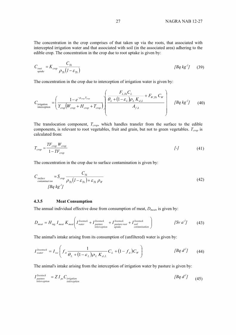
27 NAGRA NAB 12-27

The concentration in the crop comprises of that taken up via the roots, that associated with intercepted irrigation water and that associated with soil (in the associated area) adhering to the edible crop. The concentration in the crop due to root uptake is given by:

( )TkTk

Tkcrop

uptakeroot 1

CKC

ερ −= [Bq kg-1] (39)

The concentration in the crop due to interception of irrigation water is given by:

( )( )

+

−+

++−

=−

kf

WTkWLdLLL

LTkL

cropcropcropcrop

Y

A

CFK

CF

THWYeC

cropcrop

,

,,

,

onintercepti irrigation

11 ρεθµ

[Bq kg-1] (40)

The translocation component, Tcrop, which handles transfer from the surface to the edible components, is relevant to root vegetables, fruit and grain, but not to green vegetables. Tcrop is calculated from:

crop

cropcropcrop TF

WTFT

−=

1 [-] (41)

The concentration in the crop due to surface contamination is given by:

( ) WTkTkTk

Tkcrop

ioncontaminat surface 1

CSC

ρεερ +−=

[Bq kg-1] (42)

4.3.5 Meat Consumption

The annual individual effective dose from consumption of meat, Dmeat, is given by:

+++= livestock

soillivestock

uptakerootpasture

livestock

erceptionpasture

livestockwatermeatmeatingmeat IIIIKIHD

ioncontaminat

int [Sv a-1] (43)

The animal's intake arising from its consumption of (unfiltered) water is given by:

( ) ( )

−+

−+= WAL

LdLLLAwc

livestockwater CfC

KfII 1

11

,ρεθ [Bq d-1] (44)

The animal's intake arising from the interception of irrigation water by pasture is given by:

onintercepti irrigation

intCIZI pc

livestock

erceptionpasture = [Bq d-1] (45)

NAGRA NAB 12-27 28

The grazing factor for pasture, Hcrop[pasture], is calculated according to7:

]pasture[crop

cpcd]pasture[crop Y

NIZnH = [a-1] (46)

The animal's intake arising from root uptake by pasture is given by:

pasture

uptakerootpc

livestock

uptakerootpasture CZII = [Bq d-1] (47)

The animal's intake arising from soil contamination of pasture is given by:

pasturesurfacepc

livestocksoil CZII

ioncontaminat

ioncontaminat = [Bq d-1] (48)

4.3.6 Milk Consumption

The annual individual effective dose from the consumption of milk is given by:

+++= livestock

ioncontaminat soil

livestock

uptakeroot pasture

livestock

erceptionintpasture

livestockwatermilkmilkingmilk IIIIKIHD [Sv a-1] (49)

4.3.7 Egg Consumption

The annual individual effective dose from the consumption of eggs is given by:

+++= poultry

soilpoultry

uptakerootpasture

poultry

erceptionpasture

poultrywatereggseggsingeggs IIIIKIHD

ioncontaminat

int [Sv a-1] (50)

The animal's intake rate is calculated in the same way as that of cattle, but with ingestion of pasture being replaced with ingestion of grain.

4.3.8 External Irradiation

The annual individual effective dose is given by:

∑∑=

k kf

k Tkkfext A

CAGD

,

, [Sv a-1] (51)

Note that the dose coefficient used for external irradiation assumes a semi-infinite plane of uniformly contaminated top soil. The dose coefficient, G, takes into account the individual occupancy of the contaminated area, which is taken to be continuous (i.e. one year per year). The average concentration over the various soil areas is used, weighted by area.

7 Note that the conversion from days to years, nd, is explicitly included in this expression. If the calculational tool used to implement the model automatically converts between time units, then the explicit conversion can be omitted from the expression.

29 NAGRA NAB 12-27

4.3.9 Inhalation

Radionuclides can be inhaled either in their gaseous form following degassing from the soil or on suspended soil particles that have concentrations determined by the sorption on the top soil. The dose from inhalation is therefore given by:

( )( ) ∑

∑

+

−

−+=+

k k,f

k Tkk,f

AA

WTkdg

TkTk

rfffairinhgasdust A

CAlvll

1aO1aO

IHD λρε

[Sv a-1] (52)

Again, the average concentration over the various soil areas is used, weighted by area.

4.4 Exposure Factors for Food Consumption The exposure factors are defined to give a consistent representation of the habits and behaviour of an individual member of the modelled community. The exposure factors represent a closed, self-sufficient agricultural community. All foodstuffs are therefore produced locally in the modelled region so that the dose calculated is not reduced by the consumption of uncontamina-ted foodstuffs. This is represented by fixing the total annual energy intake from food con-sumption and distributing the consumption rates among the foodstuffs to give the required annual energy intake, E0 [kJ a-1]. Each of the ingestion rates in the exposure model is then defined in terms of their fractional contribution to this total:

∑=

fpathwaysfood

ff IE h0 [kJ a-1] (53)

The fractional consumption rates are then given by:

0EI

f fff

h= [-] (54)

The consumption rate of eggs, on a fresh weight basis, is given by:

=

egg

eggs

eggseggs

w

fEI

h0 [kg a-1]

(55)

The consumption rate of milk is given by:

=

milk

milk

milkmilk

w

fEI

h0 [kg a-1] (56)

The consumption rate of drinking water takes account of the consumption rate of milk and is defined as:

milkfluidwat III −= [m3 a-1] (57)

NAGRA NAB 12-27 30

The consumption rate of freshwater fish, on a fresh weight basis, is given by:

ff

ffff

fEI

h0= [kg a-1] (58)

The consumption rate of fruit, on a fresh weight basis, is given by:

fruit

fruitfruit

fEI

h0= [kg a-1] (59)

The total energy intake by vegetable consumption is taken to be8:

( )fruitffmilkeggsveggrgrrvrvgvgv ffffEpIII −−−−≡++ 10hhh [kJ a-1] (60)

The proportion of the total energy from each of the vegetable consumption pathways is given by:

( )fruitffmilkeggsveg

ii

ivegetable

ii

iii ffffEp

II

Ip−−−−

≡=∑ 10

hh

h [-] (61)

The remaining annual food energy intake is assumed to be from meat consumption:

( )( )fruitffmilkeggsvegmeat

meat ffffpEI −−−−−= 110

h [kg a-1] (62)

8 Note that gv, rv and gr are used to denote green vegetables, root vegetables and grain, respectively.

31 NAGRA NAB 12-27

5 References

Brennwald M.S. and van Dorp F. (2008). Biosphärenmodellierung in den sicherheitstechnischen Betrachtungen für die Vororientierung zum Sachplan geologische Tiefenlager. Nagra Working Report NAB 08-01.

ENSI (2009). Specific Design Principles for Deep Geological Repositories and Requirements for the Safety Case. Guideline for Swiss nuclear installations ENSI G03/e, Swiss Federal Nuclear Safety Inspectorate.

ICRP (2007). ICRP Publication 103: The 2007 Recommendations of the International Commis-sion on Radiological Protection. Annals of the International Commission on Radiological Protection (ICRP) 37/2-4, Elsevier.

Klos R.A., Müller-Lemans H., van Dorp F. and Gribi P. (1996). TAME – The Terrestrial Aquatic Model of the Environment: Model Definition. Nagra Technical Report NTB 93-04.

Nagra (2002). Project Opalinus Clay: Models, Codes and Data for Safety Assessment. Demonstration of disposal feasibility for spent fuel, vitrified high-level waste and long-lived intermediate-level waste (Entsorgungsnachweis). Nagra Technical Report NTB 02-06.

Nagra (2003). Biosphere Modelling for the Opalinus Clay Safety Assessment – Concepts and Data. Unpubl. Nagra Internal Report.

Nagra (2010). Biosphärenmodellierung: Grundlagen für die Testrechnungen. Beurteilung der geologischen Unterlagen für die provisorischen Sicherheitsanalysen in SGT Etappe 2. Nagra Working Report NAB 10-15.

Nagra (2013). Biosphere Modelling for C-14: Description of the Nagra Model. Nagra Working Report NAB 12-26.

Smith K., Sheppard S., Albrecht A., Coppin F., Fevrier L., Lahdenpera A.-M., Keskinen R., Marang L., Perez D., Smith G., Thiry Y., Thorne M. and Jackson D. (2009). Modelling the Abundance of Se-79 in Soils and Plants for Safety Assessments of the Underground Disposal of Radioactive Waste. BIOPROTA report, Version 2.0.