Arbitrage and Convergence: Evidence from Mexican ADRs

by

Samuel Koumkwa∗

and

Raul Susmel*

This Draft: June 2007

ABSTRACT

This paper investigates the convergence between the prices of ADRs and the prices of the

Mexican traded shares using a sample of 21 dually listed shares. Since both markets have

similar trading hours, standard arbitrage considerations should make persistent deviation

from price parity rare. We use a STAR model, where the dynamics of convergence to

price parity are influenced by the size of the deviation from price parity. Based on

different tests, we select the ESTAR model. Deviations from price parity tend to die out

quickly; for 14 out of 21 pairs it takes less than two days for the deviations from price

parity to be reduced by half. The average half-life of a shock to price parity is 3.1

business days, while the median half-life is 1.1 business days. By allowing a non-linear

adjustment process, the average half-life is reduced by more than 50% when compared to

the standard linear arbitrage model. We find that several liquidity indicators are

positively correlated to the speed of convergence to price parity.

JEL classification: G14, G15

Keywords: ADRs, Nonlinear Convergence, Arbitrage, ESTAR

∗ Department of Finance, C. T. Bauer College of Business,

University of Houston, Houston TX 77204-6282

skoum@yahoo.com; rsusmel@uh.edu, respectively.

1

I. Introduction

In this paper, we study the possible arbitrage opportunities that the American

Depository Receipts (ADRs) market provides. Although trading ADRs in the U.S. is U.S.

dollar denominated, it should be equivalent to trading the foreign firms’ shares without

actually trading them in their respective local markets. In the absence of direct or indirect

trading barriers, there should not be significant differences between the return distribution

of locally traded shares and that of the U.S. traded ADRs.1 That is, ADRs and their

underlying shares are expected to be perfect substitutes and no arbitrage opportunities

should prevail. If prices between the ADRs and their underlying shares differ

substantially, arbitrage opportunities will arise.

There is a substantial body of literature that studies the potential arbitrage

opportunities that the ADRs create. The early studies by Maldonado and Saunders

(1983), Kato, Linn and Schallheim (1991), Park and Tavakkol (1994), Miller and Morey

(1996) and Karolyi and Stulz (1996) concluded that ADRs do not present any arbitrage

opportunities. The only early study that did find some arbitrage opportunities is by

Wahab, Lashgari and Cohn (1992). Substantial deviations from arbitrage pricing are

consistent with other studies in the literature of dually-listed shares, such as Rosenthal

and Young (1990), and Froot and Dabora (2003). As discussed by Gagnon and Karolyi

(2003), there are impediments due to market frictions and imperfect information that can

seriously limit arbitrage. Gagnon and Karolyi (2003), however, quantify sizable price

deviations from price parity and find these deviations to exceed reasonable measures of

1 Many papers deal with the issue of international barriers to trading, investments, and cash flows

movements. See Stulz (1981), Eun and Janakiramanan (1986), Stulz and Wasserfallen (1995) and

Domowitz, Glen and Madhavan (1997).

2

the costs of exploiting them. De Jong, Rosenthal and van Dijk (2004) and Hong and

Susmel (2003) show that simple arbitrage strategies based on the deviation from

theoretical prices parity can deliver significant profits. These significant deviations from

arbitrage pricing have been attributed to market inefficiencies, see Mullainathan and

Thaler (2000) and Barberis and Thaler (2003).

The convergence to price parity has also been recently studied. Gagnon and

Karolyi (2003) discuss the mechanics of arbitrage in the ADR market. Arbitrage, which

involves the issuance and cancellation of ADRs, can take place on the same day, but it

usually occurs on an overnight basis. Gagnon and Karolyi (2003) report the average

deviation from price parity can persist for up to five days. Some studies, however, find

convergence to price parity to be surprisingly slow. For example, De Jong, Rosenthal and

van Dijk (2004) find substantial variation in the number of days for which an arbitrageur

has to maintain a position before convergence. In some cases, arbitrageurs have to wait

for almost 9 years.

In this paper, we focus on the price convergence between the ADRs and their

underlying shares. We study Mexican ADRs because the trading hours in Mexico and

New York are almost identical, thus, convergence to price parity should not be affected

by possible lead-lag informational impact, as analyzed by Kim, Szakmary and Mathur

(2000). The majority of the studies in this area have, implicitly, focused on linear

convergence to arbitrage parity.2 Given the complexity of rules, direct and indirect

transaction costs, however, non-linear adjustments to price parity deviation are more

likely to occur. We use two popular non-linear models for our adjustment specification:

2 See for instance Kim et al. (2000) for VAR and SUR approaches to analyze the speed of adjustment of

ADR prices; and Gagnon and Karolyi (2003) for a standard AR model.

3

the exponential smooth transition autoregressive (ESTAR) and the logarithmic smooth

transition autoregressive (LSTAR). From our estimation results, first, we reject the linear

adjustment model; and, second, based on different tests, we select the ESTAR model.

Using the ESTAR model, we are able to estimate the half-life of different shocks. We

find that price spreads tend to die out quickly, for 14 out of 21 firms it takes less than 2

day for the ADR-underlying price spread to be reduced by half. These results are

consistent with the dynamics of arbitrage in the ADR market. Gagnon and Karolyi (2003)

mention that although the process of issuance and cancellation of ADRs can take place on

the same day; the process usually occurs on an overnight basis. We find that for four

firms, however, the half-life estimates seem very high (seven days or more). Three of

these four firms correspond to companies that display very low volume, and thus,

arbitrage might be difficult to execute. The average half-life is 3.1 business days and the

median half-life is 1.08 days. By allowing non-linear adjustments, the average half-life

and the median half-life are reduced by more than 50%, when compared to the standard

linear model.

This paper is organized as follows. Section II presents a brief literature review.

Section III motivates the STAR model and briefly discusses estimation and testing issues.

Section IV presents the data. Section V estimates the non-linear model and analyzes the

conversion path to arbitrage parity. Section VI concludes the paper.

II. Literature Review

There is a growing body of literature that studies the potential arbitrage

opportunities that cross-listed shares create. If prices between the local shares and their

4

cross-listed shares differ substantially, arbitrage opportunities will arise. As pointed out

in the introduction, the early studies conclude that arbitrage opportunities are non-existent

for cross-listed shares and thus cross-listed shares are priced according to arbitrage parity.

The only early study that did find some arbitrage opportunities is by Wahab, Lashgari

and Cohn (1992). Some recent works, however, have found a significant deviation from

arbitrage price parity. Froot and Dabora (1999), studying the pricing of two dual-listed

companies, Royal Dutch and Shell, and Unilever N.V. and Unilever PLC, find a large

and significant price deviation from arbitrage parity. Gagnon and Karolyi (2003)

quantify sizable price deviations from arbitrage-free pricing between ADRs and their

underlying assets. Gagnon and Karolyi (2003) document the existence of large price

deviations for many of the 581 ADR-underlying pairs they study. They estimate

discounts of up to 87% and premia of up to 66%. Gagnon and Karolyi (2003), after

taking into account direct and indirect transaction costs still find the price deviations to be

exceeding reasonable measures of transaction costs. Still, they mention that the

complexity of rules in the ADR-underlying arbitrage precludes definite conclusions about

potential market inefficiencies.

Large price deviations from arbitrage-price parity do not necessarily imply

arbitrage profits are possible. Transaction costs, capital control restrictions, conversion

rules, and lack of liquidity might make arbitrage very difficult. De Jong et al.(2003) and

Hong and Susmel (2003) attempt to construct realistic arbitrage strategies to see whether

arbitrage is possible. De Jong et al. (2003) extend the sample to 13 dual-listed companies

and show that for every individual dual-listed company, deviations from arbitrage price

parity are large. They design investment strategies for exploiting these deviations from

5

price parity. They find that some arbitrage strategies in all dual-listed companies produce

excess returns of up to 10% per annum on a risk-adjusted basis, after transaction costs

and margin requirements. Hong and Susmel (2003) study simple arbitrage profits for

ADR-underlying pairs. They find that pairs-trading strategies deliver significant profits.

The results are robust to different profit measures and different holding periods. For

example, for a conservative investor willing to wait for a one-year period, before closing

the portfolio pairs-trading positions, pairs-trading delivers annualized profits over 33%.

Suarez (2005a), using intradaily data for French ADR-underlying pairs, shows that large

deviations from the law of one price are present in the data and that an arbitrage rule can

be designed to exploit the large deviation from price parity.

A related line of research deals with the price discovery process. Eun and

Sabberwal (2003) apply a standard linear error correction model to study price discovery

shares for 62 Canadian shares cross-listed in the NYSE. They find a significant price

deviation from arbitrage parity. They find that the price adjustments of U.S. prices to

deviation from Canadian prices are significantly larger in absolute value. They also find

that trading volume in the U.S. is the most important variable in the determination of

relative information contribution of the two markets. Using intradaily data and a similar

methodology, but for only three German firms, Gramming, Melvin, and Schlag (2001)

find that the majority of the price discovery is done at home (Germany), but following a

shock to the exchange rate, almost all of the adjustment comes through the New York

price. A similar model, but using non-linear adjustment dynamics, is estimated by

Rabinovitch et al. (2003). Using a non-linear threshold model for 20 Chilean and

Argentine cross-listed stocks, Rabinovitch et al. (2003) estimate transactions costs and

6

show that transaction costs play an important role in the convergence of prices of ADRs

and their underlying securities. They find that capital control measures and liquidity

significantly affect the price adjustment process, through increasing transactions costs.

Melvin (2003) and Auguste et al. (2004) also find that capital movement restrictions can

seriously affect the arbitrage price parity, especially during economic and currency crisis.

III. Non-linear convergence and Arbitrage Models

Let Pt(A) represent the price of ADRs and Pt(L) the price of underlying (locally)

traded shares a time t. The relationship between both prices, under the arbitrage-free

condition, with absence of transaction costs is specified as:

Pt(A) = B St Pt(L), (1)

where St denotes the nominal exchange rate at time t, and B the bundling price ratio.

Equation (1), price parity, is usually expressed in log form. The deviations from log price

parity, qt is given by

b sppq t

A

t

L

tt ++−≡ , (2)

where small letters represents the log form of the above defined variables. Let κ measure

the transaction costs, as a percentage, faced by arbitrageurs. Provided that κ is small,

arbitrage will occur when:

| qt | > κ (3)

The dynamic behavior of qt, the deviation from price parity between the ADRs and their

underlying shares, has been mostly analyzed in a linear framework.3 For example, Eun

3 Exceptions are in Rabinovitch et al. (2003), Chung, Ho and Wei (2005) and Suarez (2005b), where

threshold autoregressive models are used.

7

and Sabherwal (2003) use a standard error correction model. This linear framework is

counterintuitive since, once arbitrage is triggered, arbitrage opportunities may disappear

very slowly and always at the same speed. One way to address this issue is to consider

that, under certain conditions, price differences should converge faster to price parity.

This can happen when the convergence dynamics are governed by a nonlinear process.

We start by assuming that small deviations from arbitrage-free prices between ADRs and

their underlying shares may be considered negligible to generate arbitrage activities,

notably when transactions and other related trading costs are not covered by the deviation

from price parity. In this case, the deviation from price parity would behave as a near unit

root process and would not converge to parity in a linear framework. On the other hand,

when deviations from price parity are large, arbitrage activities, then, will create a

reversion to the long-run equilibrium price parity. As the ADR-underlying pair moves

further away from arbitrage parity, or long run equilibrium, arbitrage activities will likely

increase.4 Therefore, the dynamics of convergence to price parity should be influenced by

the size of the deviation from price parity.

III.1 Modeling Nonlinear Adjustments

A model that captures this nonlinear adjustment process is the smooth transition

autoregressive (STAR) model studied by Granger and Teräsvirta (1993) and Teräsvirta

(1994).5 The STAR model also displays regimes, but the transitions between regimes

4 See Dumas (1992), Uppal (1993), Sercu et al. (1995), Coleman (1995), Obstfeld and Taylor (1997). These

articles find that market frictions create an inactive transaction band, where small deviations from

purchasing power parity prevent the real exchange rate to mean revert. Arbitrage opportunities exist only

for large deviations outside the inactive band. Traders have a tendency to postpone entering the market

until enormous arbitrage opportunities open up.

5 Another popular nonlinear specification is the threshold autoregressive (TAR) model in which regime

8

occur gradually. In the STAR literature, the Exponential STAR (ESTAR) and the

Logistic STAR (LSTAR) are the most popular models used for symmetric and

asymmetric adjustments, respectively. The adjustment structure of both models depends

on the magnitude of the departure of the underlying process from its equilibrium. A

STAR model of order p for the univariate time series qt can be formulated as:

) , ;('

2

'

1 µλtttt zxxq ΦΨ+Ψ= + εt, λ> 0 (4)

or

)-(qL q tj

p

1jj1t µ∑Ψ+µ=

=+

µ∑Ψ

=) -(qL t

jp

1jj2 [ ) , ;z( t µλΦ ]+ εt, λ > 0 (4')

where the error term, εt, follows an identical and independent distribution, with zero

mean and constant variance σ2. The independent variable tx is defined as tx = (1, tx~ )’

with tx~ = (qt-1, qt-2,…,qt-p)’ and Ψi = (Ψi0, Ψi1,…, Ψip), i =1,2, denotes the

autoregressive parameters vector of dimension p of an AR(p); L is the lag operator;

) , ;z( t µλΦ is the smooth transition function, which determines the degree of

convergence. The ESTAR model uses the exponential function as the transition function6:

) , ;z( t µλΦ = { }2

z

2

t tσ̂/µ)(zexp1 −−− λ , λ> 0 (5)

where, zt, the transition variable is assumed to be a lagged endogenous variable zt = qt-d

for which d is the delay lag, a nonzero integer (d > 0), that determines the lagged time

changes occur abruptly, see Tong (1990). A problem with this approach is that the model has two very

distinct regimes: outside the threshold (where arbitrage happens) and inside the threshold (where there is no

arbitrage). The change from one regime to the other is abrupt and it presumes the same speed of adjustment

outside the threshold. The LSTAR model contains as a special case the single-threshold TAR model,

discussed in this section. 6 The sample variance of the transition variable is used to scale the argument of the exponential as

suggested by Granger and Teräsvirta (1993, p.124). The scaling enables a stability improvement of the

nonlinear least squares estimation algorithm, a fast convergence, and an interpretation and comparison of λ

estimates across equations in a scale-free environment.

9

between a shock and the response by the process, the parameter λ determines the speed of

transition between regimes, and µ can be interpreted as the arbitrage parity, equilibrium

level. Note that, for a given price parity deviation, lower (higher) values of λ determine

slower (faster) values for Φ(.) and, thus, slower regime transitions.

The transition function is symmetrical around the equilibrium level (mean).

Substituting (5) into (6), the ESTAR model can be written as:

)-(qL q tj

p

1jj1t µ∑Ψ+µ=

=+

µ∑Ψ

=) -(qL t

jp

1jj2 [ { }2

z

2

t tσ̂/µ)(zexp1 −−− λ ]+ εt (6)

or xxq t'2t

'1t Ψ+Ψ= [ { }2

z

2

t tσ̂/µ)(zexp1 −−− λ ] + εt (6’)

The transition function is bounded between zero and one. The inner regime is

characterized by qt-d = µ, when Φ(.) = 0. The ESTAR model (6) then degenerates to a

standard linear AR (p):

)-(qL q t

jp

1j

jt µΨ+µ= ∑=

+ εt. (7)

The outer regime is characterized by an extreme deviation from the price parity, when

Φ(.) = 1, in which case model (6) converts to a different AR(p) representation:

)-(qL ) ( q t

jp

1j

j2j1t µΨ+Ψ+µ= ∑=

+ εt. (8)

The model displays global stability provided ) ( p

1j

j2j1∑=

Ψ+Ψ < 1, although it is possible

that 1 p

1j

j∑=

≥Ψ implying then qt may follow a unit root process or even explodes around

the arbitrage free parity level.

10

The LSTAR model uses the logistic function, instead of an exponential function,

to model the transition function Φ(.). Thus, after substituting in (4’), the LSTAR model

can be written as:

xxq t'2t

'1t Ψ+Ψ= { })]σ̂µ)/(zexp[1/(1

tzt −−+ λ + εt, λ> 0.

III.2 Estimation, Testing and Model Selection7

Following Teräsvirta (1994), the starting point in modeling a STAR specification

consists of an adequate choice of the autoregressive parameter, p, and of the delay

parameter, d. Second, a sequence of tests of the null hypothesis of linearity (AR model) is

performed, along with other diagnostic tests. Third, if the null hypothesis of linearity is

rejected, the model is specified as ESTAR or LSTAR. The choice of ESTAR or LSTAR

model is based on a comparison of p-values for a sequence of LM tests.8

The choice of the autoregressive parameter, p, is based on the Akaike information

criterion (AIC). However, the AIC tends to under-parameterize an AR model. Thus, we

also look at the partial autocorrelation function (PACF) using a 95% confidence interval

band. In order to specify the delay parameter, d, a sequence of linearity tests is carried out

for different ranges of d with 1 ≤ d ≤ D considered appropriate. If the null hypothesis of

linearity is rejected at a pre-specified level for more than one value of d, then d is

determined at d = d* such that: d* = Arg{Min p(d)} for 1 ≤ d ≤ D, where p(d) denotes

the (p-value) of the selected test. The correct choice of d is important for the test to have

a maximum power. For this paper, we set the maximum value of d equal to 5 business

days as it seems unreasonable to argue that it would take more than 5 days for the price

7 See the Appendix for details.

8 See Van Dijk et al. (2002) for a survey of the different modeling procedures for STAR models.

11

spread to start adjusting if there is an arbitrage activity. Once p and d are selected,

estimation of a STAR model can be straightforward using non-linear least squares.

We test for the presence of nonlinearity in the price spread between the local

assets and their corresponding ADRs using the Lagrange Multiplier (LM) tests proposed

by Luukkonen et al.(1988); Granger and Teräsvirta (1993) and Teräsvirta (1994)

(hereafter, the TP procedure); and Escribano and Jordá (1999) (hereafter, the EJP

procedure). For each test, we conduct a heteroskedasticity-consistent specification since

neglecting heteroskedasticity can seriously affect the power of LM tests, see Wooldridge

(1990, 1991).9

Once a nonlinear specification is found adequate, the next task is to choose

between the ESTAR and the LSTAR models. Teräsvirta (1994) suggests the following

model selection procedure. Let LMEST

denote the F-test of the ESTAR null hypothesis,

and let LMLST

denote the F-test of the LSTAR null hypothesis. The relative strength of

the rejection of each hypothesis is then compared. If the minimum p-value corresponds to

LMLST

, the LSTAR model is selected, but if it corresponds to LMEST

, the selected model

is the ESTAR.

IV. The Data

The data analyzed in this paper are the daily prices on twenty one locally traded

firms from Mexico, obtained from Datastream. To be part of our sample, the ADR has to

9 Van Dijk et al. (1999) develop outliers-robuts tests, since they show that in the presence of additive

outliers, LM tests for STAR nonlinearity tend to incorrectly reject the null hypothesis of linearity. We used

such tests along with the heteroskedasticity tests, but there were no major changes for our sample.

12

be Level III or Level II. The sample periods are different for the different firms,

depending on the dates for which ADRs started trading on these firms on the U.S. market.

Table 1 presents the twenty one firms and the sample period for each of them.

Table 2 exhibits several statistics for each firm: Market Capitalization (MC), average

daily volume since inception (Volume), the number of freely traded shares in the hands

of the public (Float), and the short-ratio, which is calculated as the short interest for the

current month divided by the average daily volume. In the last four columns of Table 2,

we also present summary statistics for the deviations from price parity (in %):

Qt = (B St Pt(L)/ Pt(A) - 1)*100.

Analyzing the statistics for Qt, we observe evidence for autocorrelation. We also tend to

observe a negative relation between liquidity and departure from theoretical price parity:

the less liquid a stock is, the bigger the departures from price parity, as shown by the

mean and maximum and minimum statistics.

V. Results

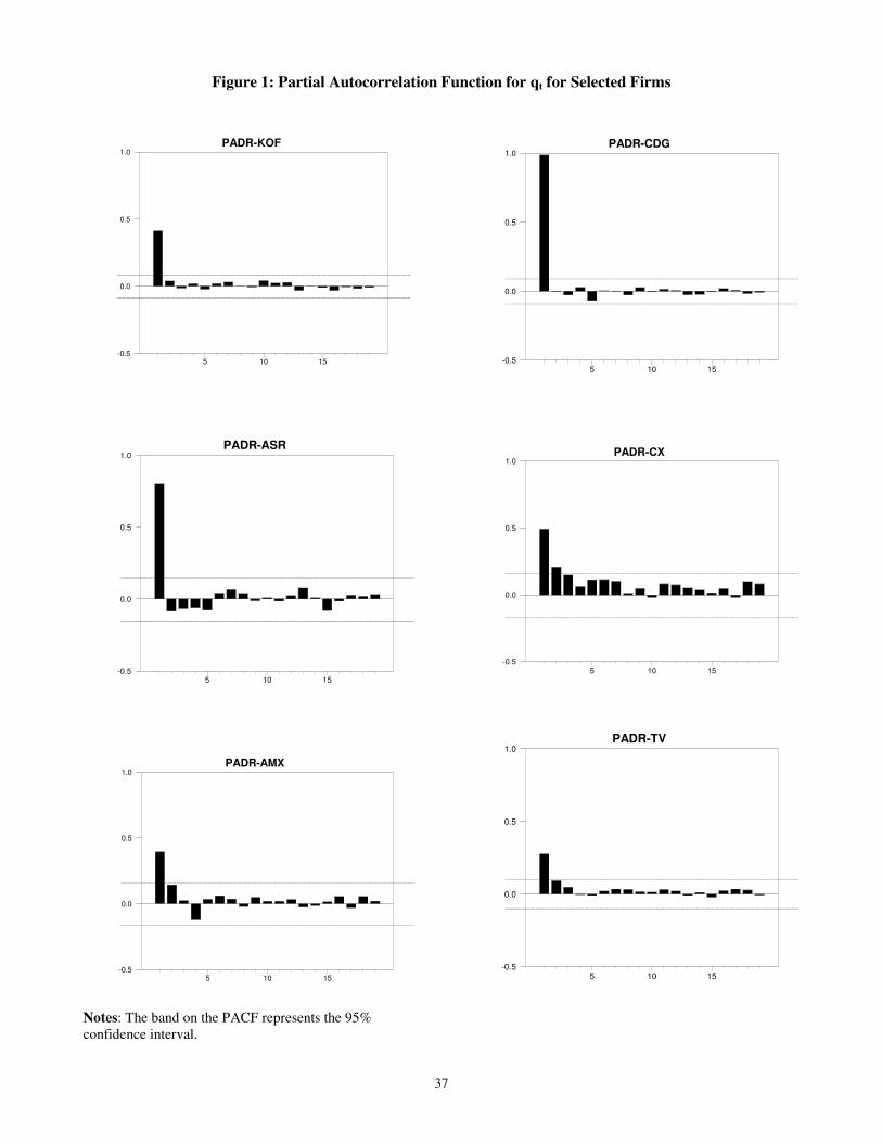
The lag selection is based on both the AIC and the partial autocorrelation

functions (PACF). Figure 1 displays the PACF for selected firms with a 95% confidence

interval band. It indicates that for most series, only the first or second autocorrelation

coefficients are significant at the 5% level. Therefore, the maximum AR used is 2, which

seems to purge the residuals series from serial correlation. As a check, we also estimate

models with p>3, with d ={1,2,…,10}, to test for a higher AR order in qt; but the results

are very similar to the ones presented below.

13

Table 3 reports p-values for the standard and heteroskedasticity-consistent test

statistics NLM3 and NLM4 for testing the linearity hypothesis. Table 3 also reports test

statistics NLM2 (an LMEST

test), LMLST

and LMEST

for choosing between ESTAR and

LSTAR (see Appendix for details). Panel A shows all the test results for one firm,

TMX.10

Panel B shows a summary of the test results for all the other firms. The second

column of Table 3 displays the different values for the delay parameter, d = {1,2,…,5}.11

Using the results on the first panel of Table 3 for TMX, we select d=2, as the results

indicate the smallest p-values (corresponding to NLM3 and NLM4) for both tests; that is,

for d=2 we obtain the strongest rejection of the AR linear hypothesis. Also, for d=2, the

ESTAR model is selected over the LSTAR model since the p-value of the LMEST

test is

smaller than the p-value of the LMLST

test, for both versions of the test. Note that the p-

value of the NLM2 test confirms this selection. We follow this process for the other

firms. Based on the standard LM test statistics NLM3 and NLM4, reported in Panel B, of

Table 3 for all the firms, the null hypothesis of linearity can be rejected for any values of

d and corresponding transition variables, at the 1% level. For the majority of the firms,

we select d=1, that is, yesterday’s deviation from price parity. When we use the

heteroskedasticity-consistent robust tests, the null hypothesis of linearity is still rejected

for the majority of the firms. Using the NLM3 test, and the lag selected by the standard

10 The results for the other firms can be reported similarly, but are not included to save space. They are

available under request. 11

The tests are performed with values of the delay parameter, d ={1,2,…,10}, yet we report the tests

statistics for d={1,2,…,5} since d={6,…,10} do not alter the choice of d and are less relevant for the

convergence of a daily price spread series. We also used as the transition variable, zt, the first lag of the

average absolute volatility, vt,k as suggested by LeBaron (1992) as: |q| k

1 v i-t

1-k

0i

kt, ∑=

= , where k is the

number of days, with a maximum of 5 business days. The tests selected vt,k as adequate transition variables

for six stocks. Overall, our results are unchanged.

14

homoscedastic test, we find eighteen firms with a p-value lower than 10%. For example,

for FMX the results of the heteroskedasticity-robust test indicate that the transition

variables zt =qt-1, qt-2, and vt-1,4 are adequate transition variables, since the corresponding

p-values are smaller than .10. The NLM3 test, for qt-1, rejects linearity, showing a p-value

of .072. The results from the NLM4 test statistic, computed using the Escribano and

Jordá test, confirm the NLM3 selection. Finally, the p-values of the LM statistics

(standard or heteroskedasticity-consistent) NLM2 suggest an ESTAR model is the more

appropriate model. Comparing relative strength of the tests LMEST

and LMLST

, the

minimum p-values correspond to LMEST

, indicating a choice in favor of the ESTAR

model. In most cases, the LMEST

is significant at the 5% level for d=1. Thus, based on the

decision rules of Teräsvirta (1994), the ESTAR model with a delay, d=1 should be an

adequate model specification for FMX return spread. We carry on an identical evaluation

for the other firms. With few exceptions we find the ESTAR to be the most adequate

model.

V.I Nonlinear Estimation Results

Following Gallant and White (1988), the resulting ESTAR(p) models, with

p={1,2}, are estimated by nonlinear least squares. We test the following restrictions

consistent with the application of ESTAR specifications to arbitrage models, Ψ11 + Ψ12 =

1, Ψj = -Ψj (j=1,2), and µ = 0. Under the first restriction, the model behaves like a

random walk, and thus there is no convergence to equilibrium, when the transition

function is equal to 0 (no arbitrage regime). Under the second set of restrictions, Ψj = -Ψj

(j=1,2), there is full convergence to price parity when the transition function is equal to 1

15

(full arbitrage regime). The last restriction, µ = 0, implies that the equilibrium price parity

deviation is zero. The restrictions are tested using likelihood ratio tests. If all the

restrictions cannot be rejected, and if imposed, the final model is governed by λ, the

speed of transition between regimes. When the last restriction cannot be rejected, we

impose it and we re-estimate the model. The model estimates, the likelihood ratio, and

residuals diagnostic statistics are presented in Table 4. In column ten, we report the p-

value associated with the likelihood ratio statistic, LR(k). The LR(k) statistics show that

at least one of the restrictions cannot be rejected at the standard 5% level for all series.

The number of restrictions that cannot be rejected varies from one firm to another. For

example for the firm AMX, the p-value of LR(4) is 0.561, thus, we failed to reject four

restrictions.12

The failure to reject the first two restrictions for AMX indicate that when

the transition function is equal to zero (no arbitrage regime) there is no tendency to

converge to price parity; on the other hand, when the transition function is equal to one

(full arbitrage regime) there is full convergence to price parity. Overall, this type of

dynamic adjustment for deviations from price parity is the usual for all the firms. That is,

we find that for small deviation from price parity there is no tendency for reversion

towards price parity; while for large deviations from price parity there is a full reversion

to price parity. The restriction µ = 0 cannot be rejected for the majority of the firms, that

is, the long-run deviation from price parity is zero. In the fourth column of Table 4, we

report the estimated λs, the transition parameters. With only one exception, TMM, the

estimates of λ are all significantly different than zero.13

The size of λ changes from 2.971

12

Ψ11+Ψ12, = 1, Ψ21 = -Ψ11, and Ψ22 = -Ψ12, and µ =0.

13 Taylor et al. (2001) point out that the significance of λ estimate based on individual t-ratios should be

checked for robustness. Technical problems emerge under the null hypothesis that λ = 0.

16

to 0.315. It is worth noticing that firms with a higher estimate of λ tend to have higher

average daily volume and market capitalization. Whereas firms for which the price

spread series exhibits a lower speed of adjustment coefficients, such as ICM (λ=0.317),

GMK (λ=0.361), and TMM (λ=0.315), tend to have lower average daily volume and

market capitalization. Overall, the estimated values reported in Table 4 support a

nonlinear dynamic convergence of the price spread series towards price parity.

We also conduct specification tests for our ESTAR model. The residuals

diagnostic statistics for the estimated equations are reported in the last two columns of

Table 4. Following Eitrheim and Teräsvirta (1996), we calculate LMNA and NLMax.

LMNA AR(1-6) is a LM-test statistics for testing the null hypothesis of no serial

correlation in the residuals of order 1, up to 6. NLMax represents the maximum LM-test

statistic of no additive nonlinearity with the delay length in the range from 3 to 6. The

associated p-values indicate that we cannot reject those null hypotheses for all firms at

the 5% level or better. Therefore, an ESTAR specification seems adequate for the price

spread series.

V.II Estimated Transition Functions

The transition function measures the magnitude of deviations of the price spread

from its arbitrage-free level. The estimates of the transition functions are shown on

Figure 2 for selected stocks; they are plotted against the transition variable, qt-d, (Panel A)

and against time (Panel B). These figures visually support the nonlinear nature of the

price spread series and the appropriateness of the ESTAR model, since, in general,

observations seem to symmetrically lie above and below the parity. Again, we notice a

17

relation between slow convergence and liquidity.14

For example, in Panel A, for a firm

with a good daily volume like KOF, a previous day’s deviation from parity of the order

plus or minus 2%, the transition function attains smaller values (0.5), implying a

relatively slow mean reversion, whereas for a larger previous day’s deviation around 4%,

the transition function reaches the value of 1, the regime of full arbitrage, signaling a

faster reversion. On the other hand, for a firm with a low daily volume TMM, a 30%

spread makes the transition function equal to .5. In general, most of the transition

functions in Panel A indicate that deviations lower than 5% trigger a full arbitrage

regime. Panel B shows that for some firms, there are few days of full arbitrage --i.e.,

when the transition function is equal to 1--, while for others, there are many days of full

arbitrage. Again, there seems to be a positive relation between low volume and number of

days under the full arbitrage regime.

V.III Half-lives and Convergence to Parity

While both estimated ESTAR models and transition functions shed lights on the

nonlinear nature of the reversion of the price spread to parity, more insights into the

adjustment mechanism of the models can be gained by estimating the average time it

takes for a given shock to die out, also called the speed of convergence to parity. As a

measure of the speed of convergence, we calculate the half-life of a shock, defined as the

number of periods it takes for shocks to the price spread to dissipate by half. Following

14

We included lagged changes in volume in the transition function, but the model did not perform better

than our model.

18

Taylor and Peel (2000) and Taylor et al. (2001), we estimated the half-lives for shocks

using the generalized impulse response function (GIRF).15

The half-life is defined in a non-linear framework as the number of periods taken

by the impulse response function to fall below 0.5 δ, or GIRF < 0.5 δ, with δ =

)1ln(100

k+ , where k represents the percentage of shocks. Alternatively, to mitigate

differences in GIRF due to the different variability of the underlying series, shocks can be

set as δ =c εσ̂ where εσ̂ denotes the residual standard deviations and c is a scalar. We use

this formulation to calculate half-lives. We estimate the half-lives for all price spread

series for three sizes of shocks: 1 εσ̂ 3 εσ̂ and 5 εσ̂ . For comparison purposes, we also

compute half-lives for a linear adjustment.

In the second to fourth columns of Table 5, we report the estimated half-lives for

all firms, using the ESTAR model, for three different sizes of shocks. In the last column,

we also report the half-life estimates for the standard AR linear adjustment model. All

half-life estimates are expressed in business days. From the non-linear estimation, we

observe faster adjustments for the majority of firms. The half-life estimates are similar

across shock sizes. A larger shock to the price spread triggers a faster reversion to parity.

For the non-linear model, using one residual standard deviation as the shock, the average

half-life is 3.1 business days, a reduction of more than half when compared to an average

half-life for the linear model of 7.26 business days. That is, we observe for all firms a

significant reduction in the half-life estimates when nonlinearities are incorporated into

15

Following Koop et al. (1996), the generalized impulse response function is defined as the difference

between two conditional first moments:

GIRFx(j, st, ωt-1) = E[Xt+j |st, ωt-1] - E[Xt+j | ωt-1], j=1,2,…,N,

where E[.] denotes the expectation operator, j is the forecasting horizon, st is the perturbation of the system

at time t, ht ≡ ωt-1 represents the conditioning information set at time t-1 consisting of the history or initial

conditions of the variable. GIRFx(j, st, ωt-1) is computed using a dynamic stochastic simulation. See also

19

the arbitrage model. These averages, however, are influenced by a few large

observations. The non-linear half-life median is 1.08 business days, also a reduction of

more than half when compared to the median half-life for the linear model of 2.29

business days. These nonlinear results are in line with the findings of Gagnon and

Karolyi (2003), where the average deviation from price parity can persist for up to five

days. Note that for 14 out of 21 firms, using the nonlinear model, it takes less than two

day for the ADR-underlying price spread to be reduced by half. The size of the shock to

price parity also matters, for 17 firms the half-life is reduced to less than 2.3 days if the

shock size is five times the residual standard deviation. Again, these results seem

consistent with the discussion in Gagnon and Karolyi (2003), where it is mentioned that

although the process of issuance and cancellation of ADRs can take place on the same

day, it usually occurs on an overnight basis.

Some of the high half-life estimates correspond to companies that display very

low volume (CDG, ICM, TMM).16

This finding is similar to the results reported in

Rabinovitch et al. (2003), where low volume is associated with higher transaction costs,

and in Roll, Schwartz, and Subrahmanyam (2004), where liquidity and lack of arbitrage

opportunities are positively related.

V.IV Nonparametric Tests of Association between Liquidity and Convergence

To formally explore whether popular indicators of a firm’s liquidity such as daily

volume, market capitalization, and float are correlated with a firm’s convergence to price

Peel and Venetis (2003a, 2003b) for a similar application to measure the half-lives of real exchange rates. 16

ICA, the other firm with a high half-life estimate, is seriously affected by a significant change in the

premium after December 3, 2003. The average premium changed from 27% to 3%. Besides a significant

investment by Mexican investor Carlos Slim, we could not find any information as to why ICA shows such

20

parity, a nonparametric Spearman rank correlation test is conducted. The null hypothesis

is that a firm’ liquidity characteristics are not related to the speed of transition between

regimes or the speed of convergence to parity against the alternative of them being

associated.

Table 6.A shows the raking of firms’ liquidity indicators, while Table 6.B shows

the Spearman rank correlations. For the non-linear adjustment model, the results indicate

that the null hypothesis of no association can be rejected at the 5% level for all liquidity

characteristics. The average daily volume, market capitalization, and float are all

positively and significantly correlated to the half-life and the speed of transition between

regimes calculated using our non-linear estimators. Our non-linear estimates provide a

better measure of liquidity than the standard linear estimates. The estimated correlations

using the non-linear half-life estimates are substantially higher than the estimated

correlations using the linear half-life estimates. For example, the correlations between

market capitalization, average daily volume and float and the non-linear half-life

estimates are .83, .58, and .66, respectively, while the correlation between the same

liquidity indicators and the linear half-life estimates are .70, .40, and .51, respectively.

VI. Conclusions

In this paper we study the convergence between the prices of ADRs and the prices

of the Mexican traded shares. We have a sample of 21 dually listed shares (listed in

Mexico and in the U.S.), that are listed as level II or level III ADRs. Since both markets

have similar trading hours, standard arbitrage considerations should make persistent

deviation from price parity rare. We estimate two different non-linear adjustment models,

a significant change in premium. ICA’s half-life estimates before and after December 3, 2003 are inline

21

the LSTAR and ESTAR models, along with a standard linear model to estimate the

convergence of the ADRs and the locally traded shares. From our estimation results, first,

we reject the linear adjustment model; and, second, based on different tests, we select the

ESTAR model. Overall, we find that for small deviation from price parity there is no

tendency for convergence towards price parity; while for large deviations from price

parity there is a full reversion to price parity. Using the ESTAR model, we are able to

estimate the half-life of different shocks to price spreads. We find that price spreads tend

to die out quickly in a nonlinear framework. The sample average half-life is 3.1 business

days, while the median half-life is 1.08 business days. By allowing non-linear

adjustments, the average half-life is reduced by more than 57%, when compared to the

standard linear model. For 14 out of 21 firms it takes less than 2 days for the ADR-

underlying price spread to be reduced by half. Four firms, however, have high half-life

estimates (seven days or more), and, in general, correspond to companies that display

very low volume, and thus, arbitrage might be difficult to execute. The results of a

Spearman correlation tests confirm this finding, as most firm’s liquidity market indicators

are positively correlated to the speed of convergence to parity. The size of the shock to

price parity also matters, for 17 out of 21 firms the half-life is reduced to less than 2.3

days when the shock size is five times the residual standard deviation.

with the rest of the firms.

22

References

Auguste, S., K. Dominguez, H. Kamil and L. Tesar, (2004), “Cross-Border Trading as a

Mechanism for Capital Flight: ADRs and the Argentine Crisis,” University of Michigan

working paper.

Barberis, N. and R. Thaler, (2002), A survey of behavioral finance, forthcoming in G.

Constantindes, M. Harris and R. Stulz, eds., Handbook of the Economics of Finance.

Coleman, A.M. (1995), “Arbitrage, Storage and the “Law Of One Price”; Mimeo,

Princeton University.

Chung, H., Ho, T. W. and L.J. Wei (2005),” The dynamic relationship between the prices

of ADRs and their underlying stocks: evidence from the threshold vector error correction

model,” Applied Economics; 37, 2387 – 2394.

De Jong, A., L. Rosenthal, and M. van Dijk, (2003), “The limits of arbitrage: Evidence

from dual-listed companies,” Erasmus University working paper.

Dickey, D. A. and W. A. Fuller, (1979) “Distribution Of The Estimators For

Autoregressive Time Series with A Unit Root,” Journal of the American Statistical

Association 74, 427-431.

Domowitz, I., J. Glen and A., Madhavan (1997b), “Market segmentation and Stock

Prices: Evidence from an Emerging Market,” The Journal of Finance, 52, 1059 – 1085.

Dumas, B., 1992, "Dynamic Equilibrium and the Real Exchange Rate in a Spatially

Separated World," Review of Financial Studies, 8, 709-742.

Dwyer, G., Locke, P., and Yu, W., (1996), “Index arbitrage and non-linear dynamics

between the S&P500 futures and cash,” Review of Financial Studies, 9, 301-332.

Escribano, A. and Jordá, O. (1999), “Improved Testing and Specification of Smooth

Transition Regression Models,” in Nonlinear Time Series Analysis of Economic and

Financial Data, Rothman, P., Kluwer: Boston, 289-319.

Eun, C. and S. Sabberwal (2002) “Cross-border listing and price discovery: Evidence

from U.S. listed Canadian stocks,” Journal of Finance 58, 549-577.

Froot, K. A. and E. Dabora, (1999) “How are Stock Prices Affected by the Location of

Trade?,” Journal of Financial Economics 53, 189-216.

Gagnon, L. and G. A. Karolyi, (2003), “Multi-market Trading and Arbitrage,”

unpublished manuscript.

23

Grammig, J., M. Melvin, and C. Schlag, (2001) “Internationally cross-listed stock prices

during overlapping trading hours: Price discovery and exchange rate effects,” Working

Paper, Arizona State University.

Granger, C.W.J. and Terasvirta, T (1993), “Modeling nonlinear economic relationships,”

Oxford University Press. Oxford, U.K.

Hong, G. and R. Susmel, (2003), “Pairs-Trading in the Asian ADR Market,” University

of Houston, unpublished manuscript.

Kato, K., S. Linn, and J. Schallheim, (1991), “Are There Arbitrage Opportunities in the

Market for American Depository Receipts?” Journal of International Financial Markets,

Institutions & Money 1, 73-89.

Karolyi, G. A., (1998), “Why do companies list shares abroad?: A survey of the evidence

and its managerial implications,” Financial Markets, Institutions, and Instruments Vol. 7,

Blackwell Publishers, Boston.

Karolyi, G. A., (2004), “The World of Cross-Listings and Cross-Listings of the World:

Challenging Conventional Wisdom,” Ohio State University, unpublished manuscript.

Koumkwa, F. Samuel (2004), “Nonlinear Dynamic Adjustment of Real Exchange Rates in

Emerging Markets,” ( Working Paper, University of Houston, Dept. Finance)

Koop, G., M. H. Pesaran, and S. M. Potter, (1996), “Impulse Response Analysis in Non-

Linear Multivariate Models,” Journal of Econometrics, 74, 119-147.

LeBaron, B. (1992), “Do moving average trading rule results imply nonlinearities in

foreign exchange markets?,” working paper, University of Wisconsin - Madison,

Madison, Wisconsin.

Lukkonnen, R., P. Saikkonen, and T. Terarsvirta, (1988), “Testing linearity against

smooth transition autoregressive models,” Biometrika, 75, 239-266.

Maldonado, W. and A. Saunders, (1983), “Foreign exchange futures and the law of one

price,” Financial Management, 12, 19-23.

Melvin, M., (2003), “A Stock Market Boom During a Financial Crisis: ADRs and Capital

Outflows in Argentina,” Economics Letters 81, 129-136.

Miller, P. D., and R. M. Morey, (1996), “The Intraday Pricing Behavior of International

Dually Listed Securities,” Journal of International Financial Markets, Institutions and

Money, 6, 79-89.

Mullainathan, S. and R. Thaler, (2000) “Behavioral economics,” MIT working paper.

24

Obstfeld, M. and M. Taylor (1997), “Nonlinear Aspects of Goods-Market Arbitrage and

Adjustment: Hecsher’s Commodity Points Revisited,” Journal of Japanese and

International Economics, 441-479.

O’Connell, Paul and Shang-Jin Wei (1997); “The Bigger They Are, The Harder They

Fall”; NBER Working Paper No. 6089, July.

Park, J., and A. Tavokkol, (1994), “Are ADRs a Dollar Translation of Their Underlying

Securities? The Case of Japanese ADRs,” Journal of International Financial Markets,

Institutions, and Money 4, 77-87.

Peel, D.A., and I. A. Venetis, (2003a), “Smooth transition models and arbitrage

consistency,” Economica.

Peel, D.A., and I. A. Venetis, (2003b), “Purchasing Power Parity over Two Centuries:

Trends and Non-linearity”, Applied Economics.

Rabinovitch, R., A. C. Silva and R. Susmel (2003) “Returns on ADRs and Arbitrage in

Emerging Markets,” Emerging Markets Review, Vol. 4, 225-328.

Rosenthal, L. and C. Young (1990), “The Seemingly Anomalous Price Behavior of Royal

Dutch/Shell and Unilever N.V./PLC,” Journal of Financial Economics 26, 123-41.

Roll, R., E. Schwartz, and A. Subrahmanyam, (2004), “Liquidity and Arbitrage,” UCLA,

working paper

Sercu, P., R. Uppal and C. Van Hulle, (1995), “The Exchange Rate in the Presence of

Transactions Costs: Implications for Tests of Purchasing Power Parity,” Journal of

Finance, 50, 1309-1319.

Suarez, E. D., (2005a), “Arbitrage opportunities in the depositary receipts market: Myth

or reality?,” Journal of International Financial Markets, Institutions and Money, 15,469-

480.

Suarez, E. D., (2005b), “Enforcing the Law of One Price: Nonlinear Mean Reversion in

the ADR Market,” 31, 1-17.

Stulz, M. R., (1981), “On the Effects of Barriers to International Asset Pricing,” Journal

of Finance, 25, 783-794.

Stulz M. R. and W. Wasserfallen, (1995), “Foreign Equity Investment Restrictions,

Capital Flight and Shareholder Wealth Maximization: Theory and Evidence,” The

Review of Financial Studies, 8, 1019 – 1058.

Taylor, N., D. van Dijk, P. Franses, and A. Lucas, (2000), “SETS, arbitrage activity, and

stock price dynamics,” Journal of Banking & Finance, 24, 1289-1306.

25

Taylor, M. P., and D. A. Peel (2000) “Nonlinear Adjustment, Long-run Equilibrium and

Exchange Rate Fundamentals,” Journal of International Money and Finance, 19, 33-53.

Terasvirta, T. (1994), “Specification, Estimation, and Evaluation of Smooth Transition

Autoregresive Models,” Journal of the American Statistical Association, 89, 208-218.

Tong, H., (1990), Threshold Models in Non-linear Time Series Analysis. Lecture Notes

in Statistics, 21. Berlin: Springer.

Uppal, R., 1993, “A General Equilibrium Model of International Portfolio Choice,”

Journal of Finance, 48, 529-553.

Van Dijk, D., T. Terasvirta, and P. H. Franses (2002), “Smooth Transition Autoregressive

Models: A Survey of Recent Developments, Econometrics Review, 21, 1-47.

Wahab, M. and A. Khandwala, (1993), “Why Diversify Internationally With ADRs?,”

Journal of Portfolio Management, 20, 75-82.

Wahab, M., M. Lashgari, and R. Cohn, (1992), “ Arbitrage in the American Depository

Receipts Market Revisited,” Journal Of International Markets, Institutions and Money, 2,

97.

Woodridge, J. M., (1990), “A Unified Approach to Robust, Regression-Based

Specification Tests,” Econometric Theory 6, 17-43.

Woodridge, J. M., (1991), “On the Application of Robust, Regression-Based Diagnostics

to Models of Conditional Means and Conditional Variances,” Journal of Econometrics

47, 5-46, January 1991.

26

APPENDIX

A.I Testing and Estimation of STAR Models

We start by rewriting equation (4’):

)-(qL q tj

p

1jj1t µ∑Ψ+µ=

=+

µ∑Ψ

=) -(qL t

jp

1jj2 [ ) , ;z( t µλΦ ]+ εt, λ > 0 (4’)

Using equation (4’), we can test the null hypothesis of linearity, by testing H0: Ψ2 = 0

against the alternative hypothesis H1: Ψ2,j ≠ 0 for at least one j ∈{0,…,p}. However,

under the null, the transition function’s parameters λ and µ are unidentified. Following

Saikkonen and Luukkonen (1988a) and Teräsvirta (1994), a third order Taylor series

expansion of the transition function Φ(qt; λ, µ) around zero is used to overcome non-

identification issues. The re-parameterization of equation (4’) yields the following

artificial regression:

tq = β00 + jt

p

1jj0 q −

=∑β + dtjt

p

1jj1 qq −−

=∑β + 2

dtjt

p

1jj2 qq −−

=∑β + 3

dtjt

p

1jj3 qq −−

=∑β + νt (A.1)

where βj = (β0j, β1j, β2j,…, βpj) with j=1,2,3 are function of the AR coefficients vector

(Ψi0, Ψi1,…, Ψip), i =1,2 and the transition function parameters λ and µ. Thus, assuming d

is known, the null hypothesis of the linearity test can be written as H0: [β1j= β2j = β3j = 0],

with j={1,2,…,p}. For large samples, the derived test statistic, NLM3, follows a

2χ distribution with (p+1) degrees of freedom. We also use the non-linearity tests

developed by Escribano and Jordá (1999) that account for the fourth power of the

transition variable. This test tries to overcome the finding that when the variance of the

error terms is large, the LSTAR (a nonlinear model) will be wrongly detected by the test

more frequently. The underlying auxiliary regression is:

27

qt = β00+ jt

p

1jj0 q −

=∑β + dtjt

p

1jj1 qq −−

=∑β + 2

dtjt

p

1jj2 qq −−

=∑β + 3

dtjt

p

1jj3 qq −−

=∑β +

+ 4dtjt

p

1jj4 qq −−

=∑β (A.2)

The null hypothesis of linearity is then: H0: β1j= β2j = β3j = β4j = 0, with j=1,…,p. The

resulting test statistic, denoted NLM4, follows a chi-squared distribution with 4(p+1)

degrees of freedom for large samples. The rejection of the null hypothesis will indicate

the presence of nonlinearity.

A.II Model Selection: Testing ESTAR vs. LSTAR

Once a nonlinear specification is found adequate, the next task is to choose

between the ESTAR and the LSTAR models. Teräsvirta (1994) suggests the use of the

artificial regression (A.1) to perform a LM test of the ESTAR specification against the

alternative of the LSTAR specification. In fact, the significance of cubic terms in

equation (A.1) will not indicate the ESTAR adjustment in that the third order Taylor

expansion of the transition function of an ESTAR model has a quadratic form (U-shape).

The cubic terms will rather signal a LSTAR type of adjustment (asymmetry). In other

words, the rejection of the null hypothesis H0L: β3j = 0 with j=1,…,p leads to the

selection of the LSTAR model, whereas the rejection of the null hypothesis H0E: β2j = 0 |

β3j = 0 with j=1,…,p leads to the selection of the ESTAR model. The test NLM2 tests

H0E. Escribano and Jordá (1999) also develop a LM-type test to discriminate between

LSTAR and ESTAR using the artificial Equation (A.2) and conditional on prior rejection

of linearity. The selection procedure is as follow: Let LMEST

denote the F-test of the null

hypothesis H0E: [β2j = β4j = 0] with j=1,…,p for ESTAR, and LMLST

the null hypothesis

28

H0L: [β1j = β3j = 0] with j=1,…,p for LSTAR. The relative strength of the rejection of

each hypothesis is then compared. If the minimum p-value corresponds to LMLST

,

LSTAR is selected, if it rather corresponds to LMEST

, the select model is ESTAR.

TABLE 1: DATA DESCRIPTION

ADR ISSUE

SYMBOL

EXCHANGE

RATIO

INDUSTRY

TYPE

EFF.DATE

AMERICA MOVIL SA

DE CV- SERIES 'L' AMX NYSE 1:20 Wireless Comm. Level II 8-Feb-01

CEMEX S.A. DE CV CX NYSE 1:5 Building Materials Level II 1-Sep-99

COCA-COLA FEMSA 'L'

SHARES KOF NYSE 1:10 Beverage Level III 1-Sep-93

CORPORACION

DURANGO CDG NYSE 1:2

Forest Products &

Paper Level III 1-Jul-94

DESC, S.A. DE C.V. DES NYSE 1:20 Auto Parts & Tires Level III 20-Jul-94

EMPRESAS ICA, S.A. DE

C.V. ICA NYSE 1:6

Heavy

Construction Level III 1-Apr-92

FOMENTO

ECONOMICO

MEXICANO, S.A. DE

C.V.

FMX NYSE 1:10 Beverage Level II 11-Feb-04

GRUMA, S.A. DE C.V. -

'B' SHARES GMK NYSE 1:4 Food Level II 6-Nov-98

GRUPO

AEROPORTUARIO DEL

SURESTE

ASR NYSE 1:10 Gen. Industrial

Svcs Level III 28-Sep-00

GRUPO IMSA IMY NYSE 1:9 Industrial

Diversified Level III 10-Dec-96

GRUPO INDUSTRIAL

MASECA S.A. DE C.V. MSK NYSE 1:15 Food Level II 17-May-94

GRUPO IUSACELL CEL NYSE 1:5 Wireless Comm. Level II 5-Aug-99

GRUPO RADIO

CENTRO, S.A. DE C.V. RC NYSE 1:9 Broadcasting Level III 9-Jul-93

GRUPO SIMEC 'B'

SHARES SIM AMEX 1:1 Mining & Metals Level III 1-Jun-93

GRUPO TELEVISA, S.A. TV NYSE 1:20 Broadcasting Level III 16-Sep-02

GRUPO TMM TMM NYSE 1:1 Industrial

Transport Level III 17-Jun-92

INDUSTRIAS

BACHOCO IBA NYSE 1:6 Food Level III 26-Sep-97

INTERNACIONAL DE

CERAMICA ICM NYSE 1:5 Building Materials Level III 15-Dec-94

TELEFONOS DE

MEXICO S.A. DE C.V.-

SERIES 'L'

TMX NYSE 1:20 Fixed Line Comm. Level III 13-May-91

TV AZTECA, S.A. DE

C.V. TZA NYSE 1:16 Broadcasting Level III 1-Aug-97

VITRO, S.A. DE C.V. VTO NYSE 1:3 Industrial

Diversified Level III 19-Nov-91

30

TABLE 2: MARKET STATISTICS

SYMBOL Volume1 MC Float2 Short

Rate2

Mean

(Qt)

SD

(Qt)

Max/Min

AR(1)

LB(5)

AMX 1,531,594 22.13B 386.70M 3.155 0.1154 1.0538 8.27/-9.46 0.391 207.31

CX 617,121 9.87B 139.84M 2.586 -0.4298 0.9613 5.44/-6.26 0.490 844.66

KOF 179,258 3.83B 27.08M 1.909 0.3720 1.8516 12.79/-9.82 0.414 615.21

CDG 23,641 55.10M 2.30M 5 16.575 58.1485 483.44/-52.00 0.988 116118.2

0

DES 50,501 665.14M 34.66M 2.667 -10.55 6.6358 14.01/-37.29 0.917 8659.15

ICA 266,505 615.47M 71.20M 16.645 -2.6896 2.4973 13.66/-17.53 0.456 1427.63

FMX 237,435 4.78B 66.26M 2.851 -0.1025 0.9973 7.56/-17.41 0.194 81.35

GMK 8,323 743.26M 21.68M 7.25 0.6519 3.9613 14.19/-81.40 0.479 758.81

ASR 130,500 587.40M 10.80M 0.407 0.8898 6.8541 86.48/-12.32 0.810 1172.07

IMY 19,590 1.13B 10.02M 9.5 0.5551 2.5380 28.56/-17.34 0.633 1842.60

MSK 33,240 397.98M 4.42M N/A 0.5484 2.4037 14.38/-29.99 0.501 1539.18

CEL 150,975 116.56M 4.72M 18.2 -0.3614 4.4567 22.51/-29.53 0.667 1291.53

RC 37,263 98.50M 8.68M 2.042 2.7286 9.3029 64.47/-24.51 0.898 8233.55

SIM 11,000 298.47M 16.10M 1.978 1.0113 11.17 77.66/-59.88 0.874 8139.64

TV 692,304 5.98B 105.89M 2.884 0.0915 1.1807 16.28/-11.14 0.267 291.30

TMM 62,341 150.38M 6.30M 16.968 -0.6590 15.3707 101.31/-68.87 0.963 12768.54

IBA 18,586 471.38M 8.17M 1.294 0.1688 2.7932 17.90/-12.13 0.702 2054.45

ICM 6,945 107.68M 5.54M N/A 3.5991 13.2577 64.95/-49.16 0.955 9441.14

TMX 2,520,634 19.09B 392.98M 8.095 0.6146 0.971 16.53/-10.86 0.305 730.84

TZA 440,805 1.49B 72.68M 7.42 -0.2084 1.4993 10.64/-10.26 0.309 259.07

VTO 164,141 304.66M 24.70M 4.636 0.3206 2.2561 14.81/-17.16 0.473 1819.54

Notes:

1. MC: Market Capitalization; Volume: average daily volume since inception, Float: number of freely traded

shares in the hands of the public. Float is calculated as Shares Outstanding minus Shares Owned by Insiders, 5%

Owners, and Rule 144 Shares. Mean(Part) is the mean of Qt= 100*(B St Pt(L) / Pt(A) -1); SD(Qt) is the SD of Qt;

Max/Min represents the maximum and the minimum of Qt; AR(1) is the AR(1) coefficient of Qt; and LB(5) is the

Ljung-Box statistics with 5 lags for Qt.

2. As of May 18, 2004. N/A: Not available

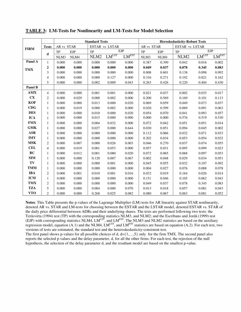
TABLE 3: LM-Tests for Nonlinearity and LM-Tests for Model Selection

Standard Tests Heroskedasticity-Robust Tests

Tests AR vs STAR ESTAR vs LSTAR AR vs STAR ESTAR vs LSTAR

TP EJP TP EJP TP EJP TP EJP FIRM

d NLM3 NLM4 NLM2 LM

LST LM

EST NLM3 NLM4 NLM2 LM

LST LM

EST

1 0.000 0.000 0.000 0.000 0.000 0.387 0.390 0.042 0.016 0.002

2 0.000 0.000 0.000 0.000 0.000 0.049 0.037 0.078 0.345 0.083

3 0.000 0.000 0.000 0.000 0.000 0.008 0.601 0.138 0.098 0.092

4 0.000 0.000 0.000 0.127 0.000 0.316 0.271 0.192 0.821 0.162

Panel A

TMX

5 0.000 0.000 0.002 0.009 0.043 0.263 0.426 0.220 0.404 0.430

Panel B

AMX 4 0.000 0.000 0.001 0.001 0.000 0.021 0.037 0.002 0.035 0.017

CX 2 0.000 0.029 0.000 0.002 0.000 0.200 0.569 0.169 0.101 0.113

KOF 1 0.000 0.000 0.013 0.000 0.020 0.069 0.059 0.049 0.073 0.037

CDG 1 0.000 0.019 0.000 0.002 0.000 0.020 0.599 0.069 0.091 0.063

DES 1 0.000 0.000 0.010 0.000 0.020 0.054 0.070 0.041 0.093 0.057

ICA 1 0.000 0.000 0.015 0.000 0.000 0.000 0.000 0.576 0.519 0.530

FMX 1 0.000 0.000 0.004 0.032 0.000 0.072 0.042 0.051 0.051 0.014

GMK 1 0.000 0.000 0.027 0.000 0.644 0.030 0.051 0.094 0.045 0.002

ASR 1 0.000 0.000 0.000 0.000 0.000 0.112 0.066 0.032 0.071 0.033

IMY 1 0.000 0.000 0.000 0.000 0.000 0.202 0.034 0.053 0.054 0.032

MSK 2 0.000 0.007 0.000 0.026 0.003 0.046 0.270 0.037 0.074 0.055

CEL 4 0.000 0.019 0.001 0.053 0.000 0.057 0.031 0.095 0.099 0.023

RC 1 0.000 0.012 0.001 0.080 0.020 0.072 0.065 0.068 0.097 0.053

SIM 1 0.000 0.000 0.120 0.007 0.067 0.002 0.048 0.029 0.034 0.051

TV 1 0.000 0.000 0.000 0.001 0.000 0.045 0.055 0.032 0.107 0.092

TMM 1 0.000 0.000 0.000 0.000 0.000 0.004 0.027 0.076 0.088 0.078

IBA 2 0.000 0.001 0.010 0.001 0.016 0.032 0.019 0.164 0.026 0.014

ICM 1 0.000 0.000 0.000 0.000 0.000 0.151 0.046 0.105 0.062 0.043

TMX 2 0.000 0.000 0.000 0.000 0.000 0.049 0.037 0.078 0.345 0.083

TZA 5 0.000 0.000 0.004 0.000 0.070 0.013 0.018 0.057 0.081 0.043

VTO 2 0.000 0.000 0.268 0.025 0.082 0.080 0.067 0.063 0.081 0.052

Notes: This Table presents the p-values of the Lagrange Multiplier (LM) tests for AR linearity against STAR nonlinearity,

denoted AR vs. STAR and LM-tests for choosing between the ESTAR and the LSTAR model, denoted ESTAR vs. STAR of

the daily price differential between ADRs and their underlying shares. The tests are performed following two tests: the

Teräsvirta (1994) test (TP) with the corresponding statistics NLM3, and NLM2; and the Escribano and Jordá (1999) test

(EJP) with corresponding statistics NLM4, LMLST

, and LMEST

. The NLM3 and NLM2 statistics are based on the auxiliary

regression model, equation (A.1) and the NLM4, LMLST

, and LMEST

statistics are based on equation (A.2). For each test, two

versions of tests are estimated, the standard test and the heteroskedasticity-consistent test.

The first panel shows p-values for all possible choices of d, d={1,…,5} only for the firm TMX. The second panel also

reports the selected p-values and the delay parameter, d, for all the other firms. For each test, the rejection of the null

hypothesis, the selection of the delay parameter d, and the resultant model are based on the smallest p-value.

TABLE 4: Nonlinear Estimation Results for ESTAR model of Price Spread

ESTAR(P): qt = µ + µ)-(qL t

jp

1j

1j∑=

ψ +

∑

=

)µ -(qL t

jp

1j

2jψ [ { }2

z

2

d-t tσ̂/µ)(qexp1 −−− λ ] + εt

FIRM p, d µ λλλλ

ΨΨΨΨ11

ΨΨΨΨ12

ΨΨΨΨ21

ΨΨΨΨ22

S

LR(k) NLMax

d={3..6}

LMNA

AR(1-6)

AMX 2, 4 - 2.745 0.842 0.155 -0.837 -0.137 0.453

LR(4) [0.498] [0.336]

(0.019) (0.106) (0.082) (0.547) (0.544) [0.561]

CX 2, 2 - 2.864 0.494 0.259 -0.470 -0.258 0.061 LR(3) [0.502] [0.452]

(0.008) (0.066) (0.046) (0.108) (0.114) [0.754]

KOF 1, 1 0.045 1.575 0.643 - - 0.612 - 0.036 LR(1) [0.471] [0.357]

(0.001) (0.025) (0.049) (0.077) [0.224]

CDG 1, 1 - 1.981 0.993 - -0.996 - 0.041 LR(3) [0.211] [0.405]

(0.528) (0.009) (0.048) [0.582]

DES 2, 1 0.163 2.971 0.921 0.164 -0.928 0.141 0.028 LR(3) [0.404] [0.471]

(0.003) (0.068) (0.050) (0.048) (0.062) (0.066) [0.672]

ICA 2, 1 -0.221 0.992 -0.765 -0.213 0.548 0.098 0.039 LR(3) [0.397] [0.545]

(0.012) (0.082) (0.113) (0.108) (0.082) (0.074) [0.423]

FMX 2, 1 - 1.793 0.865 0.147 -0.859 -0.161 0.027 LR(4) [0.438] [0.443]

(0.014) (0.011) (0.075) (0.070) (0.094) [0.522]

GMK 1,1 - 0.361 0.839 - -0.841 - 0.042 LR(2) [0.399] [0.562]

(0.039) (0.234) (0.043) [0.252]

ASR 1, 1 - 1.277 0.806 - -0.809 - 0.021 LR(2) [0.305] [0.668]

(0.027) (0.122) (0.439) [0.252]

IMY 2, 2 - 0.642 0.526 0.164 -0.535 0.160 0.048 LR(3) [0.574] [0.218]

(0.030) (0.121) (0.113) (0.109) (0.114) [0.352]

MSK 2, 2 0.025 0.582 0.897 0.175 -0.876 -0.133 0.030 LR(3) [0.327] [0.525]

(0.003) (0.053) (0.111) (0.077) (0.094) (0.083) [0.571]

CEL 2, 4 - 0.496 0.611 0.305 -0.609 -0.095 0.041 LR(3) [ 0.318] [0.280]

(0.038) (0.071) (0.066) (0.123) (0.132) [0.471]

RC 1, 2 0.211 0.835 0.876 - -0.950 -

0.038 LR(1) [ 0.390 ] [0.572]

(0.012) (0.104) (0.031) (0.043) [0.197]

SIM 2, 1 0.348 0.514 0.911 0.234 -1.09 -0.239 0.052 LR(3) [0.795] [0.489]

(0.010) (0.099) (0.084) (0.065) (0.183) (0.173) [0.458]

33

TABLE 4 : (Continued) Nonlinear Estimation Results for ESTAR model of Price Spread

FIRM p, d µ λλλλ

ΨΨΨΨ11

ΨΨΨΨ12

ΨΨΨΨ21

ΨΨΨΨ22

S

LR(k) NLMax

d={3..6}

LMNA

AR(1-6)

TV 2, 1 - 2.289 0.823 0.081 -0.824 -0.078 0.032 LR(4) [0.321] [0.254]

(0.030) (0.158) (0.139) (0.101) (0.073) [0.285]

TMM 1, 1 - 0.315 0.973 - -0.973 - 0.042 LR(2) [0.244] [0.145]

(0.737) (0.019) (0.019) [0.628]

IBA 2, 2 - 1.550 0.638 0.296 -0.641 -0.278 0.019 LR(4) [0.275] [0.323]

(0.021) (0.038) (0.031) (0.274) (0.276) [0.356]

ICM 1, 1 -0.053 0.317 0.975 - -0.846 - 0.035 LR(1) [0.399] [0.379]

(0.014) (0.094) (0.010) (0.039) [0.334]

TMX 2, 2 0.026 2.853 0.718 0.261 -0.709 -0.131 0.010 LR(3) [0.589] [0.258]

(0.001) (0.018) (0.065) (0.057) (0.456) (0.173) [0.573]

TZA 2, 5 - 1.387 0.965 0.023 -0.978 0.127 0.031 LR(3) [0.535] [0.332]

(0.013) (0.042) (0.042) (0.149) (0.135) [0.628]

VTO 2, 2 -0.037 0.984 0.771 0.156 -0.725 -0.134 0.019 LR(4) [0.419] [0.425]

(0.005) (0.093) (0.092) (0.058) (0.065) (0.048) [0.425]

Notes:

P and d denote the autoregressive order and the number of period for the delay parameter respectively. ΨΨΨΨ11, ΨΨΨΨ12,

ΨΨΨΨ21 and ΨΨΨΨ22 represent the estimated autocorrelation parameters, λλλλ the estimated speed of transition, µ the estimated

mean, and S the residual standard errors of models.

Figures reported in the squared brackets are the (p-values). ARCH tests conducted on the residuals of the estimated

models indicated the presence of heteroscedasticity. Therefore numbers in parentheses denote heteroscedastic-consistent

standard errors of estimates computed using Woodridge (1991). LMNA AR(1-6) is a LM -test statistics for testing the

null hypothesis of no serial correlation in the residuals of order 1, up to 6 developed as in Eitrheim and Teräsvirta (1996).

NLMax denotes the maximum LM- test statistic of no additive nonlinearity with the delay length in the range from 3 to 6;

they are constructed as in Eitrheim and Teräsvirta (1996). LMNA and NLMax allow the assessment of models adequacy.

LR(k) denotes a likelihood ratio test statistic for k parameters restrictions implicit to the estimated equation against the

unrestricted ESTAR model. For example, LR(4) tests the significance of the following four restrictions µ =0, Ψ11+Ψ12, =

1, Ψ21 = -Ψ11, and Ψ22 = -Ψ12.

34

TABLE 5: Speed of Convergence: Half-lives

Nonlinear Adjustment (ESTAR)a

Linear

Adjustment

(AR)b FIRM

εσ̂1 εσ̂3 εσ̂5 tq (5)

AMX 0.643 0.588 0.507 0.850

CX 0.516 0.544 0.514 2.318

KOF 0.701 0.634 0.612 0.839

CDG 10.895 10.759 9.661 50.027

DES 2.356 2.267 1.084 12.313

ICA 12.908 12.772 11.674 15.685

FMX 0.542 0.497 0.494 0.505

GMK 1.079 0.968 0.555 0.732

ASR 0.945 0.892 0.712 2.287

IMY 0.986 0.866 0.793 2.057

MSK 1.042 1.045 0.947 1.691

CEL 2.094 2.195 2.183 2.601

RC 3.616 3.527 2.344 7.014

SIM 1.893 1.846 1.008 7.363

TV 0.694 0.664 0.666 0.704

TMM 12.575 12.439 11.341 32.550

IBA 1.995 1.764 1.103 2.344

ICM 7.116 7.027 5.844 7.014

TMX 0.551 0.458 0.475 1.040

TZA 0.606 0.603 0.603 0.792

VTO 1.164 0.976 0.832 1.799

Average 3.10 3.02 2.57 7.26

Notes: All figures are in (business) days. A half-life is defined as the number of periods it takes for shocks to

pricing error to dissipate by a half. In a non-linear framework, it is such that the impulse response function is

less than unity or Gh(δ, ωt-1)<0.5

a. Half-lives for shocks εσ=δ ˆi ( i=1,3,5) where εσ̂ denotes the residual standard deviation

b. Half-lives computed in a linear framework, using the Augmented Dickey-Fuller (ADF) representation, which

regresses the first difference of the price spread qt on a deterministic component, its lagged level, and k lagged

first differences:

(1-L)qt = dt + αααα qt-1 + ∑=

k

j 1

φφφφj(1-L)qt-j + εεεεt,

where L denotes the lag operator, εt the error term, αααα, the persistence parameter, and dt the deterministic

component which can be a constant, µµµµ0, or a constant and a time trend, µµµµ0+βt, and k denotes the autoregressive

lag length. The maximum lag length in the ADF specification is set equal to 5 business days. The lag truncation

is selected using a general-to-specific methods.

35

Table 6.A: Ranks of Firms Market Characteristics

FIRM

Speed of

transition

Price

spread

Nonlinear

Half-life

Price

spread

Linear

Half-life

Average

Daily

Volume

Market

Capitalization Float

AMX 4 5 6 2 1 2

CX 2 1 12 4 3 3

KOF 8 7 5 8 6 9

CDG 6 19 21 16 21 21

DES 1 16 18 13 10 8

ICA 12 21 19 6 11 6

FMX 7 2 1 7 5 7

GMK 19 11 3 20 9 11

ASR 11 8 11 11 12 13

IMY 15 9 10 17 8 14

MSK 16 10 8 15 14 20

CEL 18 15 14 10 18 19

RC 14 17 15 14 20 15

SIM 17 13 17 19 16 12

TV 5 6 2 3 4 4

TMM 21 20 20 12 17 17

IBA 9 14 13 18 13 16

ICM 20 18 16 21 19 18

TMX 3 3 7 1 2 1

TZA 10 4 4 5 7 5

VTO 13 12 9 9 15 10

36

Table 6.B: Nonparametric Tests of Association Between Firm Market

Characteristics and Convergence to Parity: Spearman Rank Correlation Coefficient ( rs )

Average

Daily

Volume

Price

spread

Nonlinear

Half-life

Price

spread

Linear

Half-life

Market

Capitalization Float

Speed of Transition 0.627 0.513 0.223 0.633 0.651

Average Daily Volume 0.579 0.404 0.513 0.777

Price spread Nonlinear Half-life 0.810 0.826 0.655

Price spread Linear Half-life 0.702 0.505

Market Capitalization 0.852

Notes:

The Spearman rank correlation coefficient is computed using the ranks as the paired

measurements on the variables (xi, xj). The test statistic is therefore, assuming no ties in either the x or y

observations, given by:

rs = 1- 6 ∑=

N

j 1

[R(x1,j) - R(x2,j)]2/[N(N

2 - 1)], | rs | ≤ 1

* denotes significance at the 5% level. The Spearman rank statistics indicate that volume, market

capitalization, and float are positively and strongly correlated with the price spread half live and the speed

of transition. This implies the higher the average daily volume, the faster an arbitrage can be executed. This

observation remains true for market capitalization and float. Critical values of Spearman’s Rank correlation

coefficient for n=21 are: 0.368 (5%); 0.438(2.5%); and 0.521(1%).

37

Figure 1: Partial Autocorrelation Function for qt for Selected Firms

PADR-KOF

5 10 15

-0.5

0.0

0.5

1.0

--------------------------------------------------------------------------------------------------------------------------------------------------------------------------------------------------------------------

--------------------------------------------------------------------------------------------------------------------------------------------------------------------------------------------------------------------

PADR-ASR

5 10 15

-0.5

0.0

0.5

1.0

--------------------------------------------------------------------------------------------------------------------------------------------------------------------------------------------------------------------

--------------------------------------------------------------------------------------------------------------------------------------------------------------------------------------------------------------------

PADR-AMX

5 10 15

-0.5

0.0

0.5

1.0

--------------------------------------------------------------------------------------------------------------------------------------------------------------------------------------------------------------------

--------------------------------------------------------------------------------------------------------------------------------------------------------------------------------------------------------------------

Notes: The band on the PACF represents the 95%

confidence interval.

PADR-CDG

5 10 15

-0.5

0.0

0.5

1.0

--------------------------------------------------------------------------------------------------------------------------------------------------------------------------------------------------------------------

--------------------------------------------------------------------------------------------------------------------------------------------------------------------------------------------------------------------

PADR-CX

5 10 15

-0.5

0.0

0.5

1.0

--------------------------------------------------------------------------------------------------------------------------------------------------------------------------------------------------------------------

--------------------------------------------------------------------------------------------------------------------------------------------------------------------------------------------------------------------

PADR-TV

5 10 15

-0.5

0.0

0.5

1.0

--------------------------------------------------------------------------------------------------------------------------------------------------------------------------------------------------------------------

--------------------------------------------------------------------------------------------------------------------------------------------------------------------------------------------------------------------

38

Figure 2: Estimated Transition Function for

Selected Firms

Panel A: Transition Function vs. Transition Variable

Φ(Zt-d;λλλλ,,,,µ) v.s. zt-d KOF

AMX

CEL

TMX

Panel B: Transition Function vs. Time

Φ(Zt-d;λλλλ,,,,µ) v.s. t

KOF

AMX

CEL

TMX

39

Figure 2: Estimated Transition Function for

Selected Firms (continued)

Panel A: Transition Function vs. Transition Variable

Φ(Zt-d;λλλλ,,,,µ) v.s. zt-d ICM

RC

DES

TMM

Panel B: Transition Function vs. Time

Φ(Zt-d;λλλλ,,,,µ) v.s. t

ICM

RC

DES

TMM