Arbitrage and Finance

Sendhil MullainathanEconomics 2030

Fall Lecture 5

Overview

• Limits of Aribitrage• Structure of mis-pricings• Bubbles• Equity Premium puzzle• Volume

Overview

• Limits of Aribitrage• Structure of mis-pricings• Bubbles• Equity Premium puzzle• Volume

Limits of Arbitrage

• Noise trader risk– Arbitrageurs have limited horizon• Agency costs

– Problem can get worse before it gets better– Arbitrage has risk– Non-diversifiability is key• How to think about this?

• Notice beauty of this paper: – No psychology

Royal Dutch/Shell

• How do we think about non-diversifiability of this risk?

Closed End Fund Discount

Limits of Arbitrage

• Not limits of arbitrage but dangers of arbitrage• Suppose traders’ have positive feedback• What should aribtrageurs do now?

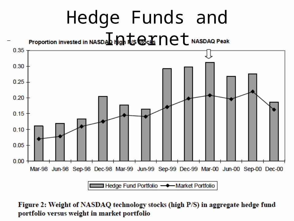
Hedge Funds and Internet

Hedge Fund Performance

Limits of Arbitrage

• Transaction costs

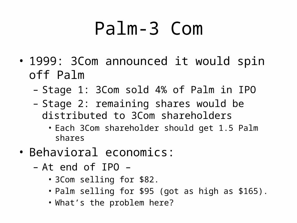
Palm-3 Com

• 1999: 3Com announced it would spin off Palm– Stage 1: 3Com sold 4% of Palm in IPO– Stage 2: remaining shares would be distributed to 3Com

shareholders• Each 3Com shareholder should get 1.5 Palm shares

• Behavioral economics:– At end of IPO –

• 3Com selling for $82. • Palm selling for $95 (got as high as $165). • What’s the problem here?

Price3Com – 1.5 PricePalm

Implementation Costs

• Implementation Costs– Commission– Bid/Ask Spread– Price Impact– Short Sell Costs• Fees• Volume Constraints• Legal Restraints

– Identification Cost• Mispricing ≠> Predictability

Limits of Arbitrage

• Noise Trader Risk• Implementation Costs• Fundamental Risk

Index Inclusions

• Stock Price Jumps Permanently– 3.5% Average

• Fundamental Risk– Poor Substitutes (best R2 < 0.25)

Limits of arbitrage

• Efficient prices vs no arbitrage• Some key questions– Best aggregator of beliefs?• Note what short-sale constraints tells us in this context• Note what arbitrage literature tells us in this context

• What would efficiency costs be?

Prediction Markets

Overview

• Limits of Aribitrage• Structure of mis-pricings• Bubbles• Equity Premium puzzle• Volume

Structure of Mispricings

• Limits of Arbitrage tells us why mispricings may occur

• The examples so far are somewhat generic• Is there structure to mispricings?

• Should there be?

Winners and Losers

Broader effect

• Not just winners and loser but also general statement about prices

Quintile A: High P/E

Quintile B Quintile C Quintile D

Quintile E: Low P/E

Median P/E

35.80 19.10 15.00 12.80 9.80

Average return

9.34% 9.28% 11.65% 13.55% 16.30%

Estimated beta

1.11 1.04 0.97 0.94 0.99

B/P E/P CF/P

Country Market Value Glamour Value Glamour Value Glamour U.S. 9.57 14.55 7.55 14.09 7.38 13.74 7.08

Japan 11.88 16.91 7.06 14.14 6.67 14.95 5.66 U.K. 15.33 17.87 13.25 17.46 14.81 18.41 14.51

France 11.26 17.10 9.46 15.68 8.70 16.17 9.30 Germany 9.88 12.77 10.01 11.13 10.58 13.28 5.14

A very different effect

Earnings Drift

When it’s realized?

Broader Version

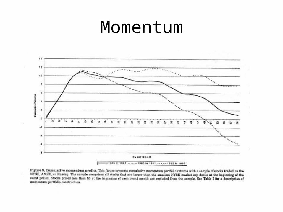
Momentum

Structure of Mispricings

• Rational Interpretation– Multi-factor models– Daniel Titman test

Structure of Mispricings

• Two sources of this structure– Arbitrage limits provide structure– Psychology of individuals provide structure

• Three prominent models– BSV– DHW– HS

Behavioral Models•Barberis, Shleifer and Vishny (1998)

•Short-term gambler’s fallacy. Updating leads to long-term hot-hand belief.

•Daniel, Hirshleifer and Subrahmanyam (1998) •A mix of biases•Confirmation(self-serving bias) leads to short-term under-reaction•Long-term over-reaction occurs because of correction

•This is an odd feature of these results.

•Hong-Stein•Limited attention and two types of traders: fundamentals and trend-chasers

•But information diffuses slowly. So diffusion creates trends which trend-chasers over extrapolate

Behavioral Models

• Lots more to be done here.• Think of the wealth of data. • Simple models with testable predictions would

be very high return.– Limited attention seems to re-appear often

Overview

• Limits of Aribitrage• Structure of mis-pricings• Bubbles• Equity Premium puzzle• Volume

Bubbles

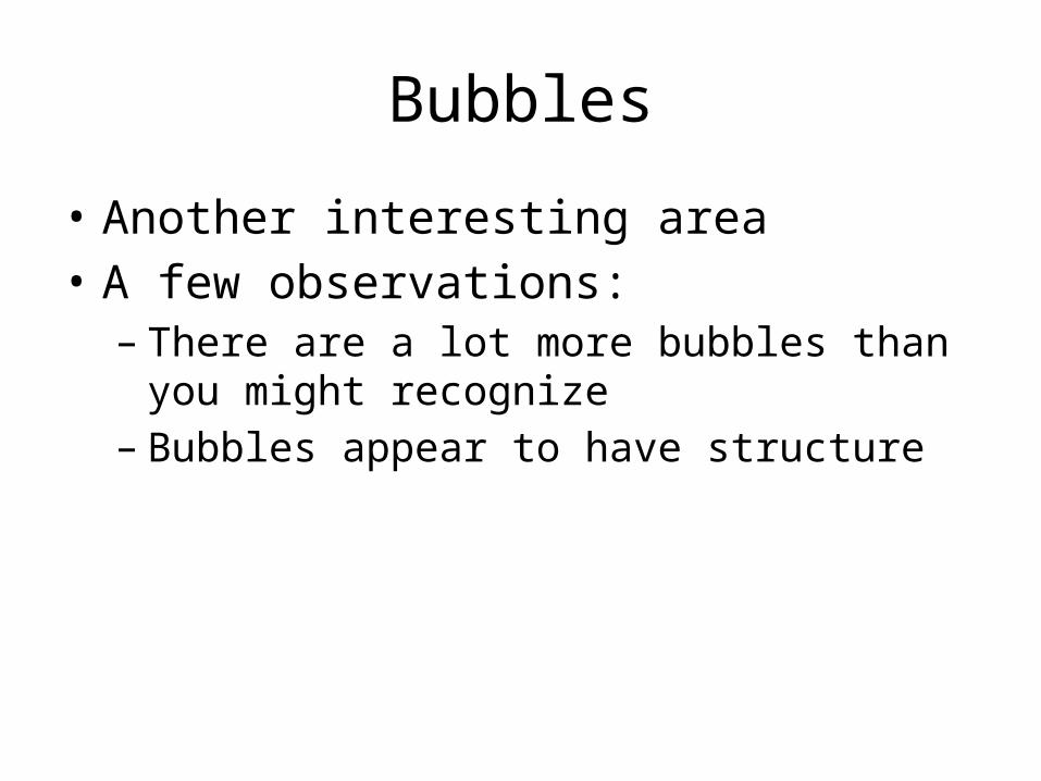
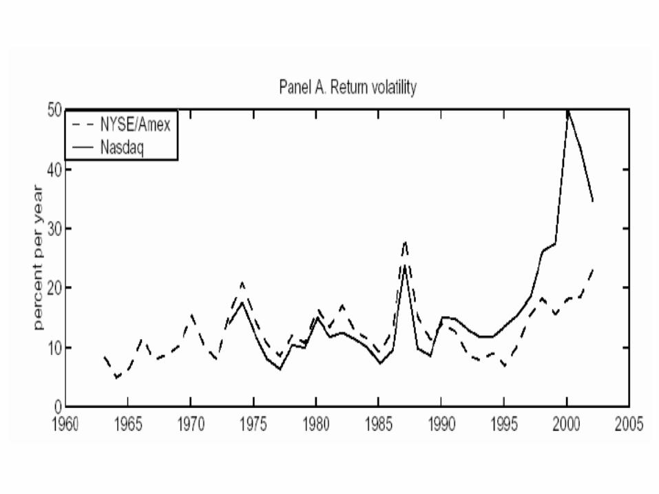
• Another interesting area• A few observations:

Bubbles

• Another interesting area• A few observations:– There are a lot more bubbles than you might

recognize– Bubbles appear to have structure

Bubbles

• Another interesting area• A few observations:– There are a lot more bubbles than you might

recognize– Bubbles appear to have structure

• Yet we have very little study of them– Are “bubbles” distinct? Or merely an arbitrary line

on a continuum?– Can we measure sentiment directly?

Overview

• Limits of Aribitrage• Structure of mis-pricings• Bubbles• Equity Premium puzzle• Volume

Consumption Model

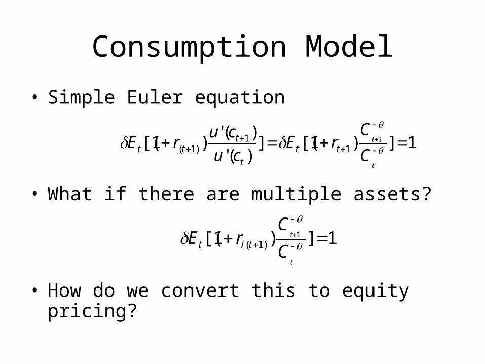
• Simple Euler equation

• What if there are multiple assets?

• How do we convert this to equity pricing?

1])1[(])('

)(')1[( 1

11

)1(

t

t

C

CrE

cu

curE tt

t

ttt

1])1[( 1

)1(

t

t

C

CrE tit

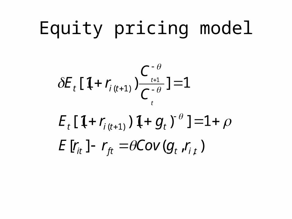
Equity pricing model

),(][

1])1)(1[(

1])1[(

,

)1(

)1(1

titftit

ttit

tit

rgCovrrE

grE

C

CrE

t

t

Calibrating this model

• Mehra Prescott, 1890-1979– Rate of return on equity is about .06– Std dev of consumption growth: .036– Std dev of stock market: .167– Correlation: .40– Covariance: .0024

• Implies: =25

Other estimates

• Mankiw Zeldes: – 1948-1988, equity premium rises to 8%– Covariance goes down– Implies =91

• A of 30 implies:– 50% chance to double wealth, 50% chance to have

wealth fall by half–Would pay 49% of wealth to avoid this gamble

Potential Explanations

• Survivorship bias– 36 exchanges, ½ had interruptions or abolished– But note: 1929 stock crash– Other evidence: international equity premium

• Learning over time– Possibly true– Equity premium may have permanently decreased– Won’t know for sure

• Limited Participation– Intermediation costs?

Observation

• Original calculations– Rate of return on equity is about .06– Std dev of consumption growth: .036– Std dev of stock market: .167– Correlation: .40– Covariance: .0024

• Which value seems low?

Epstein-Zin preferences

)1/()1(

)]([)1(

)](,[

1

111

1

1

1

ttt

ttt

UEC

UECU

• Basic idea– Suppose expected utility tomorrow also affects

utility today

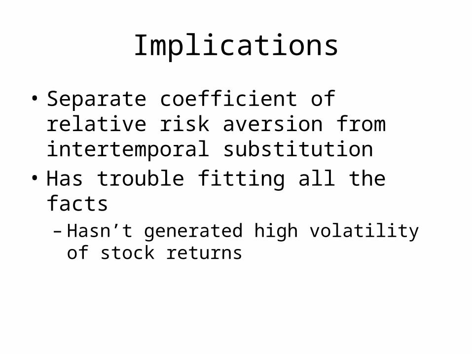
Implications

• Separate coefficient of relative risk aversion from intertemporal substitution

• Has trouble fitting all the facts– Hasn’t generated high volatility of stock returns

Potential explanation

• Perhaps consumption covaries too little with stock market growth– Nearly every explanation uses this feature in some

way

Gabaix-Laibson

–Most direct– Suppose you only adjust consumption every D

quarters.–What impact would this have to estimated equity

premium?• Show bias on estimated risk aversion is of order of 6 D

– How might you solve this problem? • Aggregate at higher horizons• Might here be some other benefit of higher level

aggregation?

Benartzi Thaler

• Investors invest in stocks and bonds• Observe performance of portfolio in time

intervals• Loss averse investors• What is the implication of variance now?– Does it depend on frequency of observation?

• How different is this from traditional risk?• Notice relation to Barberis and Xiong’s point

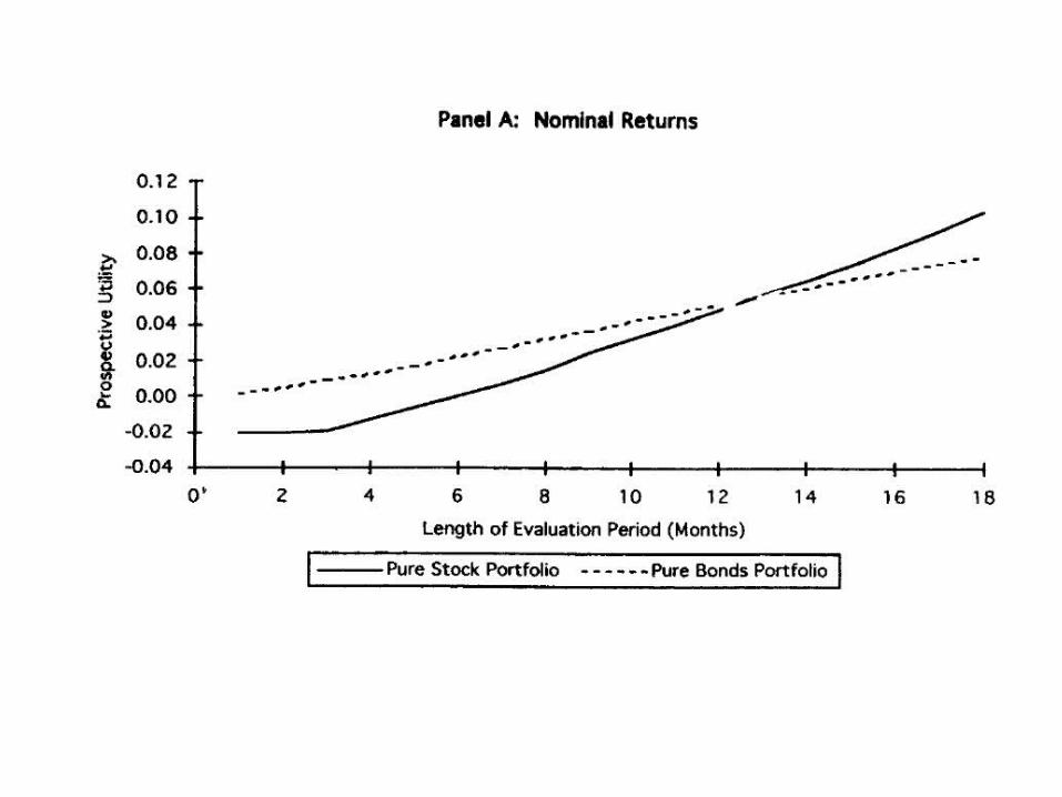
Interesting findings

• At around evaluation of year, stock and bond roughly equal– At existing equity premium.

Barberis-Huang-Santos

• Observe that in calibrations this is not enough– BT is not an equilibrium model.– Does not produce enough stock return volatility.

• How to price risk in even more?

Barberis Huang Santos

• Standard utility function in consumption• Utility over wealth

– Defined over current gains/losses (X)– Impact of S, wealth, relative to lagged reference points captured in z.

Allows changing reference points (mental accounting)– Key feature: Wealth movements matter independent of consumption

• Show they can calibrate such a model to explain equity premium.

Overview

• Limits of Aribitrage• Structure of mis-pricings• Bubbles• Equity Premium puzzle• Volume

Odean

• Looks for direct evidence of prospect theory in asset markets

• In investor behavior.

• How do they buy or sell stocks?

Other asset markets

• Genesove-Mayer examine housing markets

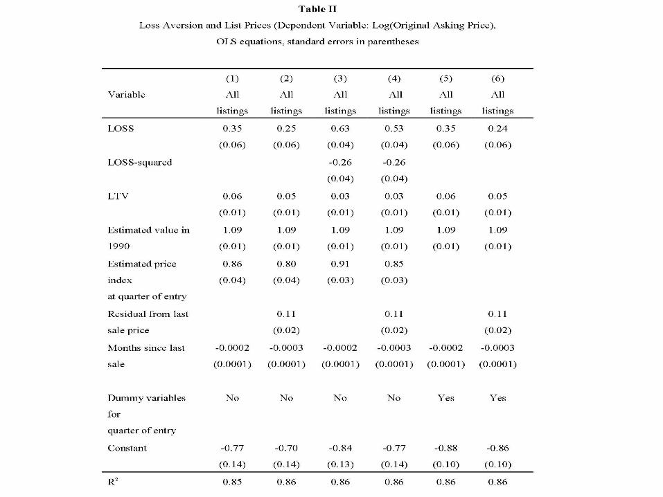
Interpretation

• Higher loss means higher selling price

• Other Facts– Higher loss means longer time to sell

– But also higher sales price

– Interesting aside: Implied return on waiting pretty high

Volume

• Deeper question– What generates so much volume?– A puzzle in and itself?

• Can we better understand disagreement– Rational models have odd features– What would a behavioral model look like?

• Have we fully exploited the structure of loss aversion?

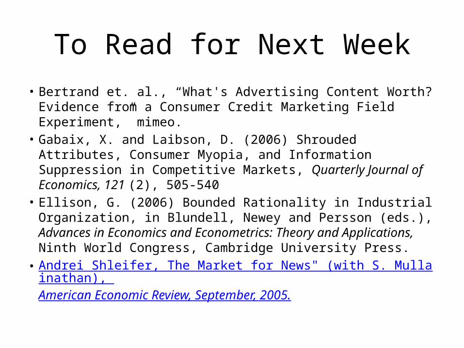
To Read for Next Week

• Bertrand et. al., “What's Advertising Content Worth? Evidence from a Consumer Credit Marketing Field Experiment,” mimeo.

• Gabaix, X. and Laibson, D. (2006) Shrouded Attributes, Consumer Myopia, and Information Suppression in Competitive Markets, Quarterly Journal of Economics, 121 (2), 505-540

• Ellison, G. (2006) Bounded Rationality in Industrial Organization, in Blundell, Newey and Persson (eds.), Advances in Economics and Econometrics: Theory and Applications, Ninth World Congress, Cambridge University Press.

• Andrei Shleifer, The Market for News" (with S. Mullainathan), American Economic Review, September, 2005.