arc geometry and algebra: foliations, moduli spaces
TRANSCRIPT

Arc Geometry and Algebra: Foliations, Moduli
Spaces, String Topology and Field Theory
Ralph M. Kaufmann∗
Purdue UniversityDepartment of Mathematics
150 N. University St.West Lafayette, IN 47907
USAemail: [email protected]
Contents
1 The spaces . . . . . . . . . . . . . . . . . . . . . . . . . . . . . . . . . . . . . 52 The gluing and the operad structures . . . . . . . . . . . . . . . . . . . . . . 113 Framed little discs and the Gerstenhaber and BV Structures . . . . . . . . . 234 Moduli space, the Sullivan–PROP and (framed) little discs . . . . . . . . . . 355 Stops, Stabilization and the Arc spectrum . . . . . . . . . . . . . . . . . . . 406 Actions . . . . . . . . . . . . . . . . . . . . . . . . . . . . . . . . . . . . . . . 477 Open/Closed version . . . . . . . . . . . . . . . . . . . . . . . . . . . . . . . 60A Glossary . . . . . . . . . . . . . . . . . . . . . . . . . . . . . . . . . . . . . . 61
Introduction
There has long been an intricate relationship between foliations, arc complexes andthe geometry of Teichmuller and moduli spaces [PH, FLP]. The study of string theoryas well as that of topological and conformal field theory has added a new aspect tothis theory, namely to study these spaces not only individually, but together all atonce. The new ingredient is the idea to glue together surfaces with their additionaldata. Physically, this can for instance be viewed as stopping and starting time for the
∗Work partially supported by NSF grant DMS 0805881

2
generation of the world–sheet. Mathematically, the general idea of gluing structurestogether in various compatible ways is captured by the theory of operads and PROPs[May1, BV, MSS]. This theory was originally introduced in algebraic topology to studyloop spaces, but has had a renaissance in conjunction with the deepening interactionbetween string theory and mathematics.
The Arc operad of [KLP] specifically provides the mathematical tool for this ap-proach using foliations. Combinatorially, the underlying elements are surfaces withboundaries and windows on these boundaries together with projectively weighted arcsrunning in between the windows. Geometrically these elements are surfaces with par-tially measured foliations. This geometric interpretation is the basis of the gluingoperation. We glue the surfaces along the boundaries, matching the windows, andthen glue the weighted arcs by gluing the respective foliations. The physical interpre-tation is that the mentioned foliations are transversal to the foliation created by thestrings. The details of this picture are given in [KP].
The gluing operation, which is completely natural from the foliation point of view,yields a surface based geometric model, for a surprising abundance of algebraic andgeometric structures germane to loop spaces, string theory, string topology, loop spacesas well as conformal and topological field theory. Surprisingly this also includes higherdimensional structures such as the little k–cubes, Associahedra, Cyclohedra and D–branes. This is true to the slogan that one only needs strings.
It gives for instance rise to models for the little discs and framed little discs operads,moduli space and the Sullivan–PROP. These models exist on the topological, the chainand the homology level. On the chain and homology these operads and PROPs corre-spond to Gerstenhaber, BV algebras, string topology operations and CFT/string fieldtheory operations. One characteristic feature is that they are very small compared totheir classical counterparts. Topologically this means that they are of small dimension.On the chain level this means that they are given by a small cellular model.
A classical result is that the little discs operad detects two–fold loop spaces, con-sequently so does the arc operad. The classical theory about loop spaces goes furtherto state that k–fold loop spaces are detected by the little k cubes or any Ek operad.This generalized to k =∞. By using a stabilization and a unital fattening of a naturalsuboperad of Arc one obtains a surface model for all these operads. A consequenceis a new infinite loop space spectrum coming from the stabilized unital fattened Arcoperad.
Another consequence of the foliation description are natural actions of the chainson the Hochschild cohomology of associative or Frobenius algebras, lifting the Gersten-haber algebra structure on the cohomology. This type of action was conjectured byDeligne and has been a central theme in the last decade. One important applicationis that this type of action together with the fact that the little discs are formal as anoperad implies Kontsevich’s deformation quantization.
There is a vast extension of this chain level action, which gives a version of stringtopology for simply connected spaces. For this the surface boundaries are classifiedas “in” or “out” boundaries. This is the type of setup algebraically described by a

3
PROP. In particular, as a generalization of the above results there is a PROP, theSullivan–PROP, which arises naturally in the foliation picture. Again there is a CWmodel for it and its chains give an action on the Hochschild co–chains of a Frobeniusalgebra extending the previous action.
This action further generalizes to a model for the moduli space of surfaces withmarked points and tangent vectors at these marked points as it is considered in confor-mal field theory and string field theory. Both these actions are given by a discretizationof the Arc operad and their algebra and combinatorics are geometrically explained byfoliations with integer weights.
Finally, there is an open/closed version of this whole theory. This generalizes theactions as well. On the topological level one consequence of this setup is for instance aclear geometric proof of the minimality of the Cardy–Lewellen axioms for open/closedtopological field theory using Whitehead moves.
Thus the Arc operad and its variations provide a wonderful, effective, geometrictool to study and understand the origin of these algebraic structures and give newresults and insights. The explicit homotopy BV equation provided by the arc operadgiven in Figure 11 or the geometric representation of the classical ∪i products in Figure17 may serve as an illustration.
We expect that this foliation geometry together with the operations of gluing willprovide new results in other fields such as cluster algebras, 2+1 dimensional TFTs andany other theory based on individual moduli spaces.
Scope
The scope of the text is a subset of the results of the papers [KLP, K2, K6, KSchw,KP, K8, K7, K5, K9] and [KP]. It is the first time that all the various techniquesdeveloped in the above references are gathered together in one text. We also makesome interconnections explicit that were previously only implicit in the total body ofresults. The main ones being the stabilization of Arc and the arc spectrum and theanalysis of the S1 equivariant geometry.
For a more self–contained text, we have added an appendix with a glossary con-taining basic notions of operads/PROPs and their algebras as well as Hochschild co-homology and Frobenius algebras.
Layout of the exposition.
In this theory there are usually two aspects. First and foremost there is the basicgeometric idea about the structure, and then secondly there is a more technical mathe-matical construction to make this idea precise. This gives rise to the basic conundrumin presenting the theory. If one first defines the mathematically correct notions, one hasto wait for quite a while before hearing the punch line. If one just presents the ideas,one is left with sometimes a formidable task to make mathematics out of the intuitive

4
notions. We shall proceed by first stating the idea and then giving more details aboutthe construction and, if deemed necessary, end with a comment about the finer detailswith a reference on where to find them.
The text is organized as follows: In the first section, we introduce the spacesof foliations we wish to consider. Here we also give several equivalent interpretationsfor the elements of these spaces. There is the foliation aspect, a combinatorial graphaspect and a dual ribbon graph version.
The basic gluing operation underlying the whole theory is introduced in section §2 asare several slight variations needed later. This leads to the Arc operad, which is a cyclicoperad. We also study its discretization and the chain and homology level operads.For the homology level, we also discuss an alternative approach to the gluing whichyields a modular operad structure on the homology level. We furthermore elaborateon the natural S1–actions and the resulting geometry. The chain and homology levelsfor instance yield new geometric examples for so–called K–modular operads.
Section §3 contains the explicit description of the little discs and framed little discsin this framework. Technically there are suboperads of Arc that are equivalent, that isquasi-isomorphic, to them. This includes an explicit presentation of the Gerstenhaberand BV structures and their lift to the chain level. In this section we give an explicitgeometric representation for the bracket and the homotopy BV equation, see Figures9 and 11.
Section §4 contains the generalization to the Sullivan–(quasi)–PROP which governsstring topology and the definition of the rational operad given by the moduli spaces.There are some fine points as the words “rational” and “quasi–” suggest which are fullyexplained.
Another fine point is that the operads as presented do not have what is sometimescalled a unit. This is not to be confused with the operadic unit that they all possess.Thus is why we call operads with a unit simply “pointed”. For the applications toString Topology and Deligne’s conjecture the operads need not be pointed. However,for the applications to loop spaces this is essential. The main point of section §5 is togive the details of how to include a unit and make the operad pointed. This allows usto fatten the Arc to include a pointed E2 operad and hence detect double loop spaces.The other basic technique given in this section is that of stabilization. The resultof combining both adding a unit and stabilization leads to the Ek operads, explicitgeometric representatives for the ∪i products (see Figure 17) and a new spectrum, theArc spectrum.
The various chain level actions are contained in §6. The first part is concerned withDeligne’s conjecture and its A∞, the cyclic and cyclic A∞ generalization. These aregiven by actions given by a dual tree picture. The section also contains the action ofthe chain level Sullivan PROP and that of moduli space on the Hochschild cochainsof a Frobenius algebra. For this we introduce correlation functions based on the dis-cretization of the foliations. As a further application we discuss the stabilization andthe semi–simple case.
We close the main text in §7 with a very brief sketch of the open/closed theory.

5
Conventions
We fix a field k. For most constructions any characteristic would actually do, butsometimes we use the isomorphism between Sn invariants and Sn co-invariants in whichcase we have to assume that k is of characteristic 0. There is a subtlety about whatis meant by Gestenhaber in characteristic 2. We will ignore this and take the algebraover the operads in question as a definition.
When dealing with operads, unless otherwise stated, we always take H∗(X) tomean H∗(X, k), so that we can use the Kunneth theorem to obtain an isomorphismH∗(X × Y, k) ' H∗(X)⊗k H∗(Y ).
1 The spaces
1.1 The basic idea
As any operad the Arc operad consists of a sequence of spaces with additional data,such as symmetric group actions and gluing maps. There are two ways in which toview the spaces:
Geometric Version: The spaces are projectively weighted families of arcs onsurfaces with boundary that end in fixed windows at the boundary considered up tothe action of the mapping class group.
An alternative equivalent useful characterization is:Combinatorial Version: The spaces are projectively weighted graphs on surfaces
with boundaries, where each boundary has a marked point and these points are thevertices of the graph, again considered up to the action of the mapping class group.
The geometric version can be realized by partially measured foliations which makethe gluing natural, while the combinatorial version allows one to easily make contactwith moduli space and other familiar spaces and operads, such as the little discs, theSullivan PROP etc..
1.2 Windowed Surfaces with partially measured foliations
We will now make precise the geometric version following [KLP].
1.2.1 Data and notation Let F = F sg,r be a fixed oriented topological surface ofgenus g ≥ 0 with s ≥ 0 punctures and r ≥ 1 boundary components, where 6g − 7 +4r + 2s ≥ 0. Also fix an enumeration ∂1, ∂2, . . . , ∂r of the boundary components of Fonce and for all.
Furthermore, in each boundary component ∂i of F , fix a closed arc Wi ⊂ ∂i, calleda window.
6
The pure mapping class group PMC = PMC(F ) is the group of isotopy classes ofall orientation-preserving homeomorphisms of F which fix each ∂i−Wi pointwise (andfix each Wi setwise).
Define an essential arc in F to be an embedded path a in F whose endpoints liein the windows, such that a is not isotopic rel endpoints to a path lying in ∂F . Twoarcs are said to be parallel if there is an isotopy between them which fixes each ∂i−Wi
pointwise (and fixes each Wi setwise).An arc family in F is the isotopy class of a non–empty unordered collection of
disjointly embedded essential arcs in F , no two of which are parallel. Thus, there is awell-defined action of PMC on arc families.
1.2.2 Induced data Fix F . There is a natural partial order on arc families given byinclusion. Furthermore, there is a natural order on all the arcs in a given arc family asfollows. Since the surface is oriented, so are the windows. Furthermore we enumeratedthe boundary components. This induces an order, by counting the arcs by starting inthe first window in the order they hit this window, omitting arcs that have alreadybeen enumerated and then continuing in the same manner with the next window.
This procedure also gives an order <i to all arcs incident to a specific boundary ∂i.
1.3 The spaces of weighted arcs
We define Ksg,r to be the semi-simplicial realization of the poset of arcs on F sg,r. This is
the simplicial complex which has one simplex for each arc family α with the i–the facemaps given by omitting the i–th arc. The dimension of such a simplex is the numberof arcs |α| minus 1. Hence the vertices of this complex correspond to the arc familiesconsisting of single arcs.
The space |Ksg,r| has a natural continuous action of PMC(F sg,r). We define Asg,r :=
|Ksg,r|/PMC(F sg,r). This space is not necessarily simplicial any more, but it remains a
CW complex whose cells are indexed by PMC orbits of arc families, which we denoteby [α]. The number of arcs is invariant under the PMC action. With the notation|[α]| := |α| the dimension of the cell indexed by [α] is |[α]| − 1.
We also consider the de-projectivized version |Ksg,r| × R>0 and its PMC quotient
Dsg,r = Asg,r × R>0.
1.4 Different pictures for arcs
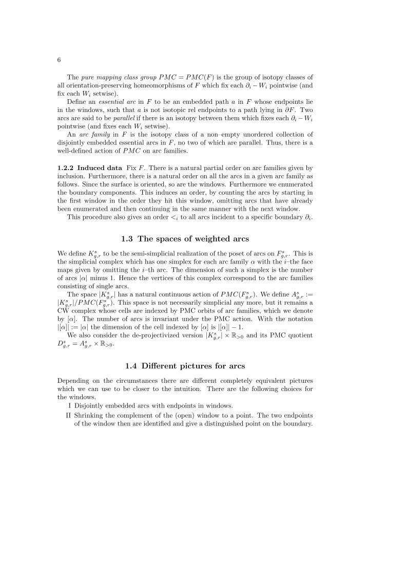
Depending on the circumstances there are different completely equivalent pictureswhich we can use to be closer to the intuition. There are the following choices forthe windows.
I Disjointly embedded arcs with endpoints in windows.
II Shrinking the complement of the (open) window to a point. The two endpointsof the window then are identified and give a distinguished point on the boundary.

7
I A
u v w wvuu v w
II A III A I B
u v w
Figure 1. I A. Arcs running to a point on the boundary; II A. Arcs running to a pointat infinity; III A. Arcs in a window; I B. Bands in a window
I C
u
v
w
wvu
II C
Figure 2. I C. Bands ending on an interval; II C. Bands ending on a circle
Arcs still do not intersect pairwise and avoid the marked points on the boundary.This version is particularly adapted to understand the S1 action (see 2.7) andthe operads yielding the Gerstenhaber and BV structures.
III Shrinking the window to a point. The Arcs may not be disjointly embedded atthe endpoints anymore, but they form an embedded graph. This is a versionthat is very useful in combinatorial descriptions, e.g. a dual graph approach formoduli spaces.
These are depicted in Figure 1. We also may choose the following different pictures forthe arcs as we discuss in 2.1 in greater detail.
A Arcs with weights.
B Bands of leaves with (transversal) width.
C Bands of leaves with width filling the windows.
The arcs with weights are the quickest method to construct the relevant spaces, thebands–of–leaves picture is what makes the operadic gluing natural. It also greatly helpselucidate the S1 action and the discretization that acts on the Hochschild complexes.
The cases I,II,III A and III B are depicted in Figure 1, the cases II B and II C arein Figure 2.

8
0
1
1
1
1
0
0
Figure 3. The space K00,2 = R as a simplicial space. We indicated two 0–simplices and
a connecting 1–simplex
1
1
0 0
1
1
1−s
Figure 4. The CW complex A00,2 = S1. We indicated the base point and a generic
element
1.4.1 Example Consider K00,2, see Figure 3. The 0–simplices are given by (the iso-
topy class of) a straight arc and all its images under a Dehn twist. Thus the 0 skeletoncan be identifies with Z. It is possible to embed two arcs which differ by one Dehn twist.Calling these one cells Iii+1, if the first arc is the i–fold Dehn twist of 0, we see that|K2
0,2| = R. PMC(F 00,2) is generated by the Dehn twist and hence A0
0,2 = R/Z = S1.This S1 is what underlies the BV geometry, see §3.
1.4.2 Elements as weighted arc families A weight function wt on an arc familyα is a map that associates to each arc of α a positive real number. There is a naturalscaling action by R>0 on the set of weight functions on α and we denote by [wt] theequivalence class of a given weight function wt under this action.
An element a ∈ |Asg,r| in the realization of Asg,r lies in a unique open simplex. Letα be the arc family indexing this simplex, then using the enumeration of arcs, we canidentify the barycentric coordinates with weights on the arcs of α. In this picture, acodimension one boundary is given by sending one of the weights to zero. We are freeto think of the barycentric coordinates as a projective class [wt] of a positive weightfunction wt on the arcs. In this fashion a = (α, [wt]).
In this picture, the elements of |Ksg,r| × R>0 are naturally pairs (α,wt) of an arc
family together with a weight function.

9
Taking the quotient by PMC, we get a description of elements of Dsg,r as pairs
([α], wt) where [α] denotes the PMC orbit of α. Further taking the quotient withrespect to the R>0 action elements of Asg,r are pairs ([α], [wt]).
1.4.3 Weights at the boundary Taking up the picture above, given (α,wt) ∈ Dsg,r,
we define the weight wt(∂i) at the boundary i of α to be the sum of the weights of theends of the arcs incident to ∂i. Notice that in this count, if an arc has both ends on ∂iits weight counts twice in the sum.
Definition 1.1. An weighted arc family ([α], wt) ∈ Dsg,r or ([α], [wt]) ∈ Asg,r is called
exhaustive if wti(α) 6= 0 for all i.We set Arcsg(r−1) ⊂ Asg,r and DArcsg(r−1) ⊂ Ds
g,r to be the subsets of exhaustiveelements.
We furthermore set Arc(n) = qg,sArcsg(n),DArc(n) = qg,sDArcsg(n) where q isthe coproduct given by disjoint union, and finally Arc = qnArc(n) and DArc(n) =qnDArc(n).
The natural Sr action descends both to Arc(r − 1) and to DArc(r − 1).
1.5 Quasi–filling families, Arc Graphs and dual Ribbon Graphs
We call an arc family quasi–filling if the complementary regions are polygons whichcontain at most one marked point.
1.5.1 Dual (ribbon) graph Let Γ(α) be the dual graph in the surface of α. Thismeans there is one vertex for every component of F \ α and an edge for each arc of αconnecting the two vertices representing the two regions on either side of the arc.
If the graph is quasi–filling this graph is again an embedded (up to isotopy) naturallyribbon graph. The cyclic order at each vertex being induced by the orientation of thesurface. The cycles of the ribbon graph are naturally identified with the boundarycomponents of F . This identification also exists in the non-quasi-filling case. Thatis the set of oriented edges or flags of Γ(α) are partitioned into cycles, that is into adisjoint union of sets each with a cyclic order.
There is an additional structure of a marking where a marking is a fixed vertexfor every cycle. This vertex is the vertex corresponding to the region containing thecomplement of the window.
Combinatorially, the vertices have valence ≥ 2 with only the marked vertices possi-bly having valence 2.
Given an element a ∈ DArc, we also obtain a metric on the dual graph of theunderlying arc family, simply by keeping the length of each edge. The geometricrealization is obtained by gluing intervals of these given lengths together at the vertices.

10
1.5.2 Arc graph It is sometimes convenient to describe the arc families simply as agraph. The basic idea is as follows: given an arc family α on F we define its graph Γ(α)to be the graph on F obtained by shrinking each window Wi to a point vi. The vi arethen the vertices and the arcs of α are the edges. We can think of Γ(α) as embeddedin F . Again there is some fine print. First the graph only has an embedding up tohomotopy. Secondly by changing the window, we changed our initial data, which isfine, but then the arcs are not disjointly embedded anymore. A rigorous geometricinterpolation of the two pictures is given in [KLP].
As an abstract graph, we can also let the vertices be given by the Wi and the edgesbe given by the set of arcs of α. In §1.6.2, we give a geometric construction of thisspace.
In the situation s = 0 and in case of a quasi–filling α the data of the marked ribbongraph Γ is equivalent to α, since one can obtain Γα by reversing the dualization.
1.6 Foliation picture
If ([α], wt) = ([{a0, a1, . . . , ak}], wt) ∈ Dsg,r is given by weights (w0, w1, . . . , wk) ∈ Rk+1
+ ,then we may regard wi as a transverse measure on ai, for each i = 0, 1, . . . , k todetermine a “measured train track with stops” and corresponding “partial measuredfoliation”, as considered in [PH].
This works as follows. Fix some complete Riemannian metric ρ of finite area onF , suppose that each ai is smooth for ρ, and consider for each ai the “band” Bi in Fconsisting of all points within ρ-distance wi of ai. Since we can scale the metric ρ toλρ, for λ > 1, we will assume that these bands are pairwise disjointly embedded in F ,and have their endpoints lie in the windows. The band Bi about ai comes equippedwith a foliation by the arcs parallel to ai which are at a fixed ρ-distance to ai, andthis foliation comes equipped with a transverse measure inherited from ρ; thus, eachcan be Bi regarded as a rectangle of width wi and some irrelevant length. The foliatedand transversely measured bands Bi, for i = 0, 1, . . . , k combine to give a “partialmeasured foliation” of F , that is, a foliation of a closed subset of F supporting aninvariant transverse measure (cf. [PH]). The isotopy class in F rel ∂F of this partialmeasured foliation is independent of the choice of metric ρ.
1.6.1 Partial Parametrization at the boundary For i = 1, 2, . . . , r, consider∂i ∩
(∐kj=0Bj
), which is empty if α does not meet ∂i and its intersection with Wi
is otherwise a collection of closed intervals in Wi with disjoint interiors. Collapse toa point each component complementary to the interiors of these intervals in Wi toobtain an interval, which we shall denote ∂i(α
′). Each such interval ∂i(α′) inherits an
absolutely continuous measure µi from the transverse measures on the bands. If ∂i(α′)
is not empty, scaling the measure to have total weight one, this gives a unique measurepreserving map of cαi : ∂i(α
′)→ S1 where S1 has the Haar measure.

11
Further collapsing the complement of the interior of Wi to a point, we get a spaceS1i (α). ci(α) induced map φi from this quotient to S1 which is a measure preserving
homeomorphism, that maps the image of the endpoints of Wi to 0 ∈ S1 = R/Z. Wecall this map the parameterized circle at ∂i.
A pictorial representation can be found in Figure 2.
1.6.2 Loop graph of an arc family: A geometric construction of the dualgraph The loop graph of a weighted arc family a ∈ DArc is the space obtained fromqiS1
i / ∼ where ∼ is the equivalence relation which is the closure of the by the relationp ≈ q if p and q are the end points of a leaf. The loop is invariant under the PMCaction and we call the resulting space L(a). There are natural maps li : S1
i → L(a),the images are called the i–th circle or lobe. The 0–th circle is also called the outsideor output circle, while the circles for i 6= 0 are called the input circles.
The loop of the graph is homeomorphic to the geometric realization of dual graphwith its metric. The circles correspond to the cycles and the marked point on eachcycle is the image of 0.
2 The gluing and the operad structures
2.0.3 Basic Idea Think of the elements of Asg,r as partially measured foliations mod-ulo common scaling. The most natural way to do this is in terms of foliations as derivedfrom the theory of “train tracks” (cf. [PH])
In this picture, two weighted exhaustive arc families can be naturally composed byfixing one boundary component on each of the surfaces and glue naturally if one gluesthe underlying surfaces along a pair of fixed boundary components. Concretely on thecondition that the weights on the two boundaries agree one produces a weighted arcfamily on the glued surface from two given arc families by viewing them as foliations.If the families are exhaustive, this can always be achieved by scaling. If one starts withprojective weights, one only chooses representatives which satisfy the condition.
This gluing yields the sought after operadic structure.
2.1 Standard gluing for foliations.
2.1.1 Basic idea Given two weighted arc families (α,wt) in F = F sg,m+1 and (β,wt′)in F ′ = F th,n+1, construct the respective foliation. Now picking one boundary compo-nent on each surface, we can glue them and the respective foliations if they have thesame weights. This is well defined up to the action of PMC.
More precisely, if the two foliations have the non–zero same weights say wti(α) =wt0(β) we can glue them to give a foliation on the surface obtained by gluing theboundary i of F to the boundary i of F ′. Identifying the glued surface with F s+tg+h,m+n
we obtain the weighted family (α,wt) ◦′i (β,wt′).

12
If we have two exhaustive weighted families, whose weights do not agree, we canuse the R>0 action to make them agree and then glue. That is in general: ([α], wt) ◦i([β], wt′) := wti(α)([α], wt) ◦′i wt0([β])(β,wt′) and this descends to Arc.
2.1.2 Gluing weighted arc families Given two weighted arc families (α,wt) inF sg,m+1 and (β,wt′) in F th,n+1 so that µi(∂i(α
′)) = µ0(∂0(β′)), for some 1 ≤ i ≤ m, wewill define a weighted arc family (γ,wt′′) := (α,wt) ◦i (β,wt′) for each 1 ≤ i ≤ m onthe surface F s+tg+h,m+n as follows:
First, let’s fix some notation: let ∂i denote the i–th boundary component of F sg,m+1,and let ∂′0 denote the 0–the boundary component of F th,n+1. We glue the boundaries
together using the maps to S1 given above. This yields a surface X homeomorphic toF s+tg+h,m+n, where the two curves ∂i and ∂′0 are thus identified to a single separating
curve in X. There is no natural choice of homeomorphism of X with F s+tg+h,m+n, but
there are canonical inclusions j : F sg,m+1 → X and k : F th,n+1 → X.We enumerate the boundary components of X in the order
∂0, ∂1, . . . , ∂i−1, ∂′1, ∂′2, . . . ∂
′n, ∂i+1, ∂i+2, . . . ∂m
The punctures are enumerated simply by enumerating the ones on Fsg,m+1 first.
Choose an orientation-preserving homeomorphism H : X → F s+tg+h,m+n which pre-serves the labeling of the boundary components as well as those of the punctures, ifany.
In order to define the required weighted arc family, consider the partial measuredfoliations G in F sg,m+1 and H in F th,n+1 corresponding respectively to (α′) and (β′).By our assumption that µi(∂i(α
′)) = µ0(∂0(β′)), we may produce a correspondingpartial measured foliation F in X by identifying the points x ∈ ∂i(α′) and y ∈ ∂0(β′)
if c(α)i (x) = c
(β)0 (y).
The resulting partial measured foliation F may have simple closed curve leaveswhich we must simply discard to produce yet another partial measured foliation F ′ inX.
The leaves of F ′ thus run between boundary components of X and therefore, as inthe previous section, decompose into a collection of bands Bi of some widths wi, fori = 1, 2, . . . , I, for some I. Choose a leaf of F ′ in each such band Bi and associate toit the weight wi given by the width of Bi to determine a weighted arc family (δ′) in Xwhich is evidently exhaustive. Let (γ′) = H(δ′) denote the image in F s+tg+h,m+n underH of this weighted arc family.
Lemma 2.1. The PMC(F s+tg+h,m+n)-orbit of (γ′) is well-defined as (α′) varies over a
PMC(F sg,m+1)-orbit of weighted arc families in F sg,m+1 and (β′) varies over a PMC(F th,n+1)-
orbit of weighted arc families in F th,n+1.
Proof. Suppose we are given weighted arc families (α′2) = φ(α′1), for φ ∈ PMC(F sg,m+1),
and (β′2) = ψ(β′1), for ψ ∈ PMC(F th,n+1), as well as a pair H` : X` → F s+tg+h,m+n of

13
homeomorphisms as above together with the pairs j1, j2 : F sg,m+1 → X` and k1, k2 :F th,n+1 → X` of induced inclusions, for ` = 1, 2. Let F`,F ′` denote the partial measuredfoliations and let (δ′`) and (γ′`) denote the corresponding weighted arc families in X`
and F s+tg+h,m+n, respectively, constructed as above from (α′`) and (β′`), for ` = 1, 2.Let c` = j`(∂0) = k`(∂
′i) ⊆ X`, and remove a tubular neighborhood U` of c` in X` to
obtain the subsurface X ′` = X` −U`, for ` = 1, 2. Isotope j`, k` off of U` in the naturalway to produce inclusions j′` : F sg,m+1 → X ′` and k′` : F th,n+1 → X ′` with disjoint images,for ` = 1, 2.
φ induces a homeomorphism Φ : X ′1 → X ′2 supported on j′1(F sg,m+1) so that j′2 ◦φ =Φ ◦ j′1, and ψ induces a homeomorphism Ψ : X ′1 → X ′2 supported on k′1(F th,n+1) sothat k′2 ◦ ψ = Ψ ◦ k′1. Because of their disjoint supports, Φ and Ψ combine to give ahomeomorphism G′ : X ′1 → X ′2 so that j′2 ◦ φ = G′ ◦ j′1 and k′2 ◦ ψ = G′ ◦ k′1. We mayextend G′ by any suitable homeomorphism U1 → U2 to produce a homeomorphismG : X1 → X2.
By construction and after a suitable isotopy, G maps F1∩X ′1 to F2∩X ′2, and thereis a power τ of a Dehn twist along c2 supported on the interior of U2 so that K = τ ◦Galso maps F1 ∩U1 to F2 ∩U2. K thus maps F ′1 to F ′2 and hence (δ′1) to (δ′2). It followsthat the homeomorphism
H2 ◦K ◦H−11 : F s+tg+h,m+n → F s+tg+h,m+n
maps (γ′1) to (γ′2), so (γ′1) and (γ′2) are indeed in the same PMC(F s+tg+h,m+n)-orbit.
Notice that although the gluing is local on the boundaries, there is a global effectof gluing the leaves together. For instance there can be bands which have both endson the same boundary. If these are split, they may recursively cut other bands. Anexample of such a gluing is given in Figure 5. Alternatively, one can describe thegluing procedure purely combinatorially, see [K3] for the details. For this one uses aleast common partition of the unit interval, duplicates each edge for every cut and thenglues the flags or half edges if they are indexed by the same subinterval.
Remark 2.2. An alternative to discarding the simple closed curve leaves is to enlargethe space Asg,r to include them. This would be in the spirit of V. Jones’ planar algebras[J]. We however do not take this route and the applications such as string topology donot exhibit these type of curves.
2.1.3 Symmetric group actions On Ksg,r there is a natural action of the symmetric
group of r elements Sr which permutes the labels 0, . . . , r−1 enumerating the boundarycomponents. It contains a subgroup Sr−1 which only permutes the labels 1, . . . , rkeeping 0 fixed. Like above, after renumbering, we have to choose a homeomorphismto the standard surface. In the figures, this is usually suppressed.
2.1.4 Comments on the details, see [KLP] Notice that since we fixed the sur-faces F sg,r the gluing actually depends a priori on a choice of homeomorphism of the

14
a cbb
f
ed
d
a
d d
b c b
e
d)
b)a)
c)
Figure 5. a) The arc graphs which are to be glued assuming the relative weights a,b,c,dand e as indicated by the solid lines in c). b) The result of the gluing (the weights areaccording to c). c) The combinatorics of cutting the bands. The solid lines are theoriginal boundaries, the dotted lines are the first cuts, and the dashed lines representthe recursive cuts. d) The combinatorics of splitting and joining flags.

15
glued surface. These choices become irrelevant after passing to PMC quotients. Otherpossibilities are to choose models F sg,r and compatible morphisms of surfaces gluedfrom these back to the chosen models.
2.1.5 Partial/Colored operad structure
Proposition 2.3. The gluings together with the symmetric group action permutingthe labels give a (cyclic) partial operad structure to the spaces D(r − 1) := qg,sDs
g,r.Moreover this partial operad structure is an R≥0 colored operad. Here R≥0 is consideredwith the discrete topology.
Proof. Notice that Sn naturally acts on D(n) via permuting the labels 1, . . . , n on theboundaries. Moreover Sn+1 acts by permuting the labels on the boundaries 0, . . . , n.The gluings if defined are associative and symmetric group equivariant; for the precisedefinition of the various actions, see the Appendix. The important point is that thegluing did not depend on the name of the boundaries. This is a straightforward check.The additional equation for a cyclic operad is also easy to check. The only obstructionto gluing is that the weights on the two boundaries which are glued are the same. Theprocedure also works if the two boundaries are both not hit by any arc. Thus assigningthe color wt(∂i) ≥ 0 to each i we obtain an R≥0 colored operad.
2.2 Cyclic Operad Structure: The scaling approach of [KLP]
In the gluing operation above, we could compose two weighted arc families if they hadthe same weight at the designated boundaries. We can get rid of this restriction ifwe consider exhaustive families by using the R>0 scaling action. Given exhaustive arcfamilies ([α], [wt]) ∈ Arc(n) and ([β], [wt′]) ∈ Arc(m)
([α], wt) ◦i ([β], wt′) := wti(α)([α], wt) ◦′i wt0([β])(β,wt′) (2.1)
Theorem 2.4. [KLP] The spaces DArc(n) form a cyclic operad and this cyclic operadstructure descends to Arc(n)
Proof. One has to recheck the associativity for this case, but it again works out [KLP].
Remark 2.5. Notice that if we start in Arc there are unique representatives ([α], wt) ∈D(n) and ([β], [wt]) ∈ D(m) such that wt(∂i) = wt′(∂0) = 1 and we could have usedthese to define gluing directly on Arc, but that would have not allowed us to lift theoperad structure to DArc.
2.2.1 Discretization: The Suboperad of positive integer weights/multiarcs

16
Proposition 2.6. The arc families in DArc with positive integer weights for a cyclicsuboperad. Using the inclusion N ⊂ R, they also form an N colored cyclic suboperad ofthe R-colored version of DArc.
A useful pictorial realization of an arc family with positive integer weights is toreplace an arc of weight k by k parallel arcs.
Alternatively, one adds k − 1 parallel copies to the arc after say fixing a smallrectangular neighborhood of the original arc. We will call positively multi–arc families.
These multi–arc families are what is used in the string topology and moduli spaceactions. There they will appear in their N colored version.
Another relevant operad structure is the one sums of these elements given as follows:Given an exhaustive arc graph α, with arcs e1, . . . ek, let α(n1,...,nk) ∈ DArc for ni ∈ Nbe defined by wt(ei) = ni
αN = q~n∈Nkα~n (2.2)
We furthermore for two exhausting arc graphs, we set
αN ◦i βN =
′∑(~n,~m)
α~n ◦i β ~m (2.3)
where∑′
runs over the pairs (~n, ~m) such that wt(∂i(α~n) = wt(∂0(β ~m), that is those
pairs for which the N–colors match.
Proposition 2.7. The compositions ◦i are operadic. Furthermore dropping the su-perscript N they give an operad structure to the collection of exhaustive arc graphs αwhere the operad degree is the number of boundaries of α.
2.3 Chains and Homology
One basic question is how operads behave with respect to functors of homology andvarious chain functors. It is the homology level that gives the algebra and the chainlevel is basically the “algebra up to homotopy” level which is relevant for applicationsfrom Deligne’s conjecture to field theory.
2.3.1 Operads and Functors: technical details The general answer to the ques-tion what kind of functor pushes forward an operad structure is that it should be aweak monoidal one. Let us denote this functor as F : C → D where both C andD are monoidal categories with a product ⊗. The condition of weakly monoidalmeans among other things (see e.g. [Kas]) that there are natural morphisms F(X,Y ) :

17
F(X)⊗F(Y )→ F(X ⊗ Y ). For our operads this means that we get compositions ◦Fiby using the sequence of maps
◦Fi : F(O(n))⊗F(O(m))F(O(n),O(m))−→ F(O(n)⊗O(m))
F(◦i)−→ F(O(m+ n− 1))
2.4 Singular Homology and Singular Chains
If we take (singular) homology with coefficients in a field k then the Kunneth formulaguarantees us that the functor H∗( , k) is even a strong monoidal functor, that is thereis an isomorphism H∗(O(n), k) ⊗H∗(O(m), k) ' H∗(O(n) ×O(m), k) and this showsthat the homology is again a cyclic operad. For singular chains the Eilenberg–Zilbertheorem provides us with a weak monoidal functor on the chain level.
Corollary 2.8. The singular chains and the homologies of DArc(n) and Arc(n) formcyclic operads.
2.4.1 Other Chains There may be other chain models besides singular chains, wemight want to use. For singular chains one has to use the Eilenberg–Zilber theorem.This is for instance easier to track in cubical chains. Mostly we will be interested ineither singular or cellular chains. Throughout we will denote singular chains by S∗ andcellular chains by CC∗. When dealing with CW complexes one has the extra bonus ofproving that the topological compositions indeed give rise to cellular maps.
Additionally in some particular cases one may obtain special chain models thatwork for a given operad in a special situation, although there is no general a prioriguarantee that the construction is valid. This then of course can and has to be checkeda posteriori.
We will just use Chain to denote any operadic chain model. In all the models weconsider, one has families representing the chains. We will from now on treat familiesand leave open the specification of a particular chain model. We will mostly use singularor cellular chains in the following.
2.5 Open/Cellular Chains
Arcsg(n) (unlike DArc) is a subspace of the CW complex Asg,r. That complex has cellsC[α] indexed by classes of arc graphs α. For Asg,r and the partial gluing structure, wecan use cellular chains. Some of the suboperads/PROPs of Arc actually have homotopyequivalent CW models whose cellular chains are models for them on the chain level.These will give us the solution to Deligne’s conjecture and it generalizations up to andincluding String Topology.
Unfortunately Arc itself is not outright a CW complex, since the condition of beingexhaustive is not necessarily stable under removing arcs. We can however regard thecomplex CC∗(A
sg,r, A
sg,r \ Arcsg(r − 1)).

18
Alternatively, Arcsg(r− 1) is also the disjoint union of open cells and hence filteredby using the dimension of cells.
Arcsg(r − 1) = q[α]:[α] is exhaustiveC[α] (2.4)
where C denotes the open cell. And although we can not use cellular chains, we canwork with the free Abelian group generated by the open cells which is denoted byC∗o (Arcsg(r − 1)). Each generator is given by an oriented cell. Such a cell is givenin turn by an arc graph. The dimension is the number of arcs minus 1. There is adifferential, which deletes arcs, as long as the result is still exhaustive. In order to getan operad structure on C∗o (Arc), we recall the following facts from [K3]:
As sets
C[α] ◦i C[β] = qΓ∈I([α],[β])C[γ] (2.5)
where I([α], [β]) is a finite index set of arc graphs on the glued surfaces [K3] runningthrough all the graphs that appear as the underlying graphs of the composed families.
If α has k arcs and β has l arcs then, if two conditions are met, for any weights,generically the number of arcs in ([α], [wt]), ([β], [wt′]) is k+ l− 1. The two conditionsare that (1) there are no closed loops and (2) that not both arc families are twisted atthe boundary at which they are glued. In these cases, the dimension of the composedcell drops. Overall the composition respects the filtration by dimension. Moreover,the “bad” part, that is the locus, where the families glue together to form familieswith less than the expected graphs is of codimension at least 1, if the two families arenot twisted at the boundary simultaneously. In that case the number of arcs in thecomposition generically already has one less arc than expected. In the top dimensionthe composition map is bijective.
The best way to treat the operadic structure is to pass to the associated gradedGrC∗o (Arc) of C∗o (Arc).
In [K3] we showed that
Theorem 2.9. The Abelian groups C∗o (Arc)(n) =∐g,s C∗o (Arcsg(n)) and GrC∗o (Arc) =∐
g,sGrC∗o (Arcsg(n)) =∐g,s CC∗(A
sg,r, A
sg,r \ Arcsg(r − 1)) are cyclic operads. Where
the compositions are given by
C(α) ◦k C(β) =∑i∈I±C(γi) (2.6)
where ± is the usual sign corresponding to the orientation, and I is a subset of I(α, β).More precisely: (1) I is empty if both families are twisted at the glued boundaries (2) Iruns over the arc graphs which are not obtained by erasing arcs and (3) in the gradedcase Gr, the arc family also has the expected maximal number of arcs.
2.5.1 Discretizing the Chain level When dealing with the chain level and theactions, there are two modifications for the discretization (2.3). The first is to addappropriate signs. The signs are given in [K4] and are discussed in the appendix. Here

19
we will just use the fact that such appropriate signs exist. The second is to adjust thegluing to fit with that of relative chains, that is to use the modification (1) and or (2)of Theorem 2.9. On the discrete side, there is again a filtration by the degree of theunderlying arc family.
For the action we will use the following
Theorem 2.10. [K4] For α an arc graph with k arcs, let
P(α) :=∑~n∈Nk
±αn (2.7)
with the appropriate sign. Then for two arc graphs: P(α ◦i β) = ±P(α) ◦i P(β), whereagain ± denotes the appropriate sign and the two ◦i are taken with the same modifica-tion. In particular using both modifications for the gluing P gives an operad morphismfrom C∗o (Arc) to the operad of N–weighted arc families (modified with appropriate signs,see [K4]0. Using the respective associated grading on the discrete P gives an operadmorphism from CC∗(A
sg,r, A
sg,r \ Arcsg(r − 1)) to the associated graded.
Remark 2.11. Here α◦iβ is the gluing given by gluing the open cells and enumeratingthe indexing set of the resulting cells. A priori this can be any gluing between twoboundaries that are hit, bu also between two empty boundaries. With the obviousmodification this applies as well to gluing an empty boundary to a non–empty one byerasing.
2.6 Modular structure: The [KP] approach.
One can ask if there is a modular operad structure for Arc. The challenge is to addself–gluings. One can readily see that the partial operad structure on the D(n) is indeedmodular. One can glue any two boundary components on connected or disconnectedsurfaces as foliations in the above manner, if the weights on the two boundaries agree.It is not possible in general, however, to scale in order to obtain self–gluings withoutrestrictions, at least on the topological level. The reason for this is that the R>0 actionscales the weights on all boundaries simultaneously, so if they don’t agree one cannotchange them to agree merely by the action.
There is however a flow, which one can use, to make them agree. This is a very in-tricate procedure, that even works in families. It is contained as one result in [KP]. Wewill content ourselves with just stating the main result as it pertains to the discussionhere.
Theorem 2.12. The homologies H∗(DArc(n)) = H∗(Arc(n)) form a modular operadusing g as the genus grading. Moreover, it is induces from a modular operad structureup to canonical homotopies on the chain level. That structure is obtained from the R>0
colored topological operad structure on DArc(n) via flows.

20
[ht!]
11
1
= 1
s
1ïs
1ïs s
I II
Figure 6. I, the identity and II, the arc family δ yielding the BV operator
2.7 S1 action
We have already seen that A00,2 ' S1. Since all the elements are exhaustive in this
case, we obtain that Arc20(1) = A00,2. We now show that this is even true as groups.
2.7.1 Group structure Pick two elements ∆t,∆s with s, t ∈ [0, 1) as depicted inFigure 4. Gluing them together there are two situations, (i) s+t ≤ 1 or (ii) 1 < s+t > 2.In the first case we immediately see that ∆t◦1∆s = ∆s+t; in the second situation we seethat after gluing the outer two strands become parallel and indeed ∆t ◦1 ∆s = ∆s+t−1.
Now via gluing there is an (S1)×n+1–action on each Arcsg(n). Let us enumerate theCartesian Product of (S1)×n+1 as having factors 0, . . . , n. Then the factors i = 1, . . . nact via ρi(t)([α], [wt]) = [α], [wt]) ◦i ∆t and the 0 component acts as ρ0(t)([α], [wt]) =∆t ◦0 [α], [wt]).
2.7.2 S1 action as twisting and moving the base point. If we look at the arcpicture II B or C, in the enumeration 1.4, we can nicely describe the geometry of thisaction. It simply moves the basepoint around the boundary in the direction of itsorientation. The distance is given by the transverse measure of the bands as in §2.1.If the basepoint moves into a band, it simply splits it.
Definition 2.13. An arc family is called untwisted at a boundary i if no two arcs areparallel after removing the base point of the boundary I in picture II. Otherwise it iscalled twisted at i. The elements of Asg,r and Arcsg(n) are twisted or untwisted if theirunderlying arc families are. We will also say an arc family is twisted or untwisted ifarcs become parallel or not after removing all basepoints at the boundaries.
In the pictures II B and C we can see the twisting more explicitly. An element istwisted at i, if the basepoint of ∂i is inside a band which is not split at the other end.

21
An example of a twisted arc family is given by ∆t. This is even the general case inthe following sense.
Lemma 2.14. Any element of Arcsg(n) lies in the orbit of an untwisted element underthe (S1)n+1 action.
Proof. Just use the action to slide the basepoints at the different boundaries out ofany band they might be inside of. In this way we obtain an element which is untwistedat each boundary. Now it can happen that there are arcs which become parallel onlyafter removing both the basepoints of the boundaries they run between. In this case,we can move the points in sync outside of the band.
Proposition 2.15. There is an action of (S1)×n+1 on Arc(n).
Proof. The action is given by (θ0, . . . , θn)α = (· · · ((∆θ0 ◦1 α) ◦1 ∆θ1) · · · ) ◦n ∆θn).The fact that this is indeed an action follows from the associativity of the operadiccompositions.
We denote the coinvariants by Arc(n)S1 .
2.8 Twist gluing
There is an additional gluing we can perform which yields an odd structure on thechain and the homology level. This is inspired by string field theory and it gives riseto a second type of Gerstenhaber and BV structure on the homology and chain levels.For this we let ∆ be the chain given by I → Arc(1); t 7→ ∆t. Notice that this chainrepresents a generator of the homology H1(Arc00(1)).
Definition 2.16. Given two chains α ∈ S∗(Arc(n)) and β ∈ S∗(Arc(m)) we define thetwist gluing α•iβ to be the chain obtained from the map ∆n×I×∆m → Arc(m+n−1)given by α ◦i ∆ ◦1 β.
Theorem 2.17. On the chain and homology level the operations ◦i induce the structureof an odd cyclic operad. Furthermore, H∗(Arc(n)) is an odd modular operad aka. aK–modular operad.
Likewise the chains on the S1 co–invariants Arc(n)(S1) form an odd cyclic operadand H∗(Arc(n)S1) is an odd modular operad.
Proof. It is easy to see that on the chain level the twist gluing is of degree 1, which isprecisely what we need for the odd versions of the operadic structures. This immedi-ately shows the first two claims. Notice that the S1 coinvariants do not form an operadby themselves. To define the gluings, we simply choose representatives, glue and takecoinvariants again. This is independent of choices, since any two lifts differ by an S1
action on the boundaries and these get absorbed into the family.

22
Corollary 2.18. The direct sums of cyclic group coinvariants⊕
n(H∗(Arc(n)))Cn+1
and⊕
n Chain(Arc(n))Cn+1carry a Gerstenhaber bracket and that of Sn+1 coinvari-
ants⊕
nH∗(Arc(n))Sn+1 carries a BV operator.The analogous result holds for the S1 coinvariants.
2.9 Variations on the gluings
We have already deviated a bit from the original gluing to obtain the modular structureon homology. There are several other variations on the basic gluing, which are necessaryand helpful. Usually these do not alter the picture on the level of homology.
2.9.1 Local scaling In the gluing of DArc we scaled both surfaces in order to obtainan associative structure. To make the two weights match, we could also just locallyscale the width of only those bands incident to ∂i(F ) and/or those incident to ∂0(F ).In fact for gluing disjoint surfaces this is exactly done by the first type of flow in [KP].What happens in this case is that the gluings are not associative any longer, but thereis a homotopy between the two different ways to compose. This guarantees a bona fideassociative structure on homology. It is rather surprising that in several situations,notably that of string topology, there are already strictly associative chain models, —see §3.3 and §4.3.2 below.
2.9.2 Erasing We have not discussed how to glue a boundary of weight 0 with one ofnon–zero weight. The natural idea is to simply erase all bands incident to the boundarywhich is glued. Indeed this is sometimes the answer. There are two caveats however.First, this operation is again not associative. Second one has to be careful that iteratingsuch gluings one does not obtain an empty arc family. One such undesirable situationoccurs when on tries to use this type of gluing to extend the operad structure to theAsg,r. Then one could obtain an empty family, but adding it would entail making thespaces contractible and hence kill all homology information.
However this type of gluing is used in string topology. The trick here is that theempty family does not appear due to the conditions that are placed on the graphs tomake them part of the Sullivan PROP.
2.9.3 Wilting The last modification is that instead of erasing, one lets the leaveswilt. Technically this can be formalized by adding wilting weights at the boundary.A wilting weight is an assignment of a length in R≥0 to each interval of ∂i \Wi. Thesource of the map ci is then the full interval with the induced measure. For the sourceof the map L , we contract the intervals just as before. The effect on the maps li isthat they are stationary on these intervals.
A foliation interpretation is as follows: on top of the foliation on the surface, we alsoconsider a compatible germ of a trivial transverse measured foliation of a neighborhoodof each boundary. Here trivial means that all leaves are homotopic to a meridian of

23
the cylinder. Compatible means that the restriction of the given partially measured ofthe surface is a sub–foliation. The other leaves are called wilted leaves. Notice thatthe weight can be zero, which means that the band is empty.
For the gluing of these foliations we use the modified maps ci and proceed as before.Upon gluing regular leaves to wilted leaves, the leaves wilt and are erased from thesurface foliation, but kept for the foliations near the boundaries which are not glued.This gluing is used in section 5.1 to add units.
3 Framed little discs and the Gerstenhaber and BV Structures
3.1 Short overview
One extremely important feature of the Arc operad is that it contains several sub–operads that are quasi–isomorphic to classically important operads. The main onesare spineless cacti which are equivalent to the little discs, cacti which are equivalent tothe framed little discs and the corrolas which are equivalent to the tight little intervalssuboperads.
The first two structures are responsible for Gerstenhaber and BV algebras on thehomology level. This is what gives rise to string topology brackets and operators aswell as solutions to various forms of Deligne’s conjecture. In our approach we get aversion of these algebras up to homotopy on the cell level which has all homotopiesexplicitly given. One nice upshot is the new symmetry of the BV equation whichnow manifests itself as a completely symmetric 12 term identity which is geometricallynicely described by a Pythagorean like triangle, see Figure 11.
On the topological level these operads give rise to loop space structures. Going a bitfurther the stabilization of the Arc operad gives rise to a filtered sequence of so–calledEk, k ∈ N ∪ {∞}, operads. These detect k-fold loop spaces respectively infinite loopspaces, see the Background section 3.1.1 below.
Without the stabilization Arc contains a E2 in the form of spineless cacti and anE1 operad in the form of corollas, both which are defined below.
There is one technical detail, namely, whether or not to include a 0 component inthe operad. We will call operads with such a component pointed.1 For the chain leveland the algebraic structures it is enough to have the non–pointed version of E2. Forthe topological level and e.g. loop space detection it is necessary to have the pointedversions. For this one has to enlarge the setup by “fattening” the operads. The detailsare given in §5.1.
Theorem 3.1. The Arc operad contains suboperads Cor, Cact and Cacti. Cor is anE1 operad that is it is equivalent to the little intervals, Cact is an E2 operad equivalent
1Another common name for these are unital operads. This is however confusing, since this couldalso mean that there is a unit in the 1 component of the operad. This is the case for all the operadswe consider.

24
to the little discs, Cacti are equivalent to the framed little discs. This is as non–pointedoperads.
Corollary 3.2.
(1) On the topological level: Any algebra over the group completion of FatCor is ofthe homotopy type of a loop space. Any algebra over the group completion ofFatCact is of the homotopy type of a double loop space. Any algebra over thegroup completion of FatArc is of the homotopy type of a double loop space.
(2) On the homology level: Any algebra over H∗(Cact) is a Gerstenhaber algebra.Any algebra over H∗(Cacti) is a BV algebra. Any algebra over H∗(Arc) is a BValgebra.
(3) On the chain level: Any algebra over Chain(Cor) is a homotopy associativealgebra. Any algebra over Chain(Cacti) is a homotopy Gerstenhaber algebraAny algebra over Chain(Cacti) is a homotopy BV algebra. Any algebra overChain(Arc) is a homotopy BV algebra.
(4) Cellular chains: For Cor, Cact and Cacti there exist CW–models where the up tohomotopy structures of the relevant algebras are given by explicit chains.
3.1.1 Background One role of linear operads, that is those based on (complexesof) vector spaces, is that they can encode certain algebraic structures. Among theseare associative, commutative, Lie, but also more complicated algebras like pre–Lie,Gerstenhaber algebras and BV algebras. We will say that an operad represents a typeof algebra, if the algebras over this operads are precisely of the given type. For a vectorspace to be an algebra over an operad means that for each element of the operad thereis an associated multi-linear operation and these operations are compatible with all theoperad structures.
Moreover some of these linear operads are actually the homology of a topologicaloperad. This provides the geometric reason for the appearance of certain types ofalgebras. If the topological operad acts on a space at the topological level, the homologyof this operad acts on the homology of this space. This provides algebraic structureson these homologies. In this type of setup it is clear that one can replace the operadby a different one if they have the same homology operad. The correct notion for thistype of equivalence is the one induced by quasi–isomorphism. One of the questionsthat arises is to what extent linear actions can be lifted to the chain or topologicallevel. On the chain level we are dealing with a dg structure and the algebras are of thetype of the algebra over the homology, but only up to homotopy.
The two classical examples we will consider are the little discs and the framed littlediscs.
Theorem 3.3. [C, Gz] An algebra is a Gerstenhaber algebra if and only if it is analgebra over the homology of the little discs operad D2.
An algebra is a Gerstenhaber algebra if and only if it is an algebra over the homologyof the framed little discs operad fD2.

25
On the topological level the relevant theorems are:
Theorem 3.4. [St, BV, May1] A connected space has the homotopy type of a loopspace if and only if it is an algebra over the A∞ operad with base point.
If a connected space is an algebra over an Ek operad, it has the homotopy type of ak–fold loop space, for k ∈ N ∪ {∞} with base point.
Here the Ek are the little k–cubes operads and being an Ek operad means that theoperad is equivalent to an Ek operad. For instance the little discs are an E2 operad.There is a subtlety here wether or not to include the base point, see §5.1.
The Arc operad itself contains E0, E1 and E2 operads as well as the framed versions.To obtain the higher Ek operads one can stabilize as in [K7] and §5.1. We will now makethe structures present inArc explicit. Note that this gives an explicit chain level versionof these operads which in turn gives explicit∞ or better “up to homotopy”–versions ofthe respective algebras. That is for example an explicit notion of Gerstenhaber algebraup to homotopy or BV algebra up to homotopy. These explicit up to homotopy versionsare extremely adapted to describe natural actions. This is one of the “miracles” of thetheory: “The geometry of foliations chooses the correct algebraic model”.
The Sullivan quasi–PROP is a rigorous incarnations of the idea of Chas–Sullivan onstring topology. This is a PROP up to homotopy, which contains homotopy versions ofthe two suboperads above. It is designed to furnish even more operations on homologyof loop spaces. This meshes well with the above results. In particular, we will exhibitsuch an action by using the Hochschild co–chain approach. The main Theorem being
Theorem 3.5. [Jo, CJ] If M is a simply connected manifold then
H∗(LM) ' HH∗(S∗(M), S∗(M))
.
The fact that the suboperads act are versions of Deligne’s Hochschild conjecture.We will give the details below.
3.2 (Framed) little discs and (spineless) Cacti
The operad of framed little discs appears as a suboperad as follows.
Definition 3.6. The operad Cacti is the suboperad of DArc given by the surfaces withweighted arc families, which satisfy
(1) g = s = 0
(2) there are only arcs which run from ∂0 to ∂i, where i 6= 0.
The operad Cact is the suboperad of Cacti where additionally
(3) For any two arcs e1, e2 incident to ∂i with e2 <i e1 we have e1 <0 e2.

26
The operad Cor is the suboperad of Cact where each element has exactly one arcper boundary i > 0 that runs to the boundary 0.
Theorem 3.7. [K1] The operad Cacti as well as its image in Arc are equivalent tothe framed little discs operad.
The operad Cact as well as its image in Arc are equivalent to the little discs operad.
Remark 3.8. The theorem about Cacti was first stated by Voronov. This and thetheorem for Cact were proven in [K1]. The method of proof is to show that there isa forgetting map, which essentially fills in the nth boundary component and that thismap is a quasi–fibration. The proof itself is quite subtle and lengthy.
Remark 3.9. These are not the original definitions of Cacti and Cact. These weregiven in [Vo2] and [K1]. They are however isomorphic operads as shown in [KLP, K1].In [KLP] the images of these operads in Arc where called T ree and LTree.
Immediate consequences are:
Corollary 3.10.
(1) The Arc operads detects loop spaces. That is: a connected space that is algebraover the Arc operad has the homotopy type of a two–fold loop space.
(2) The group completion of the Arc operad has the homotopy type of a double loopspace.
3.2.1 Cactus terminology. One arrives at the usual pictures, resembling succulents,if one considers the images under the loop map L or the dual graphs. The conditions(1) and (2) translate to the fact that this graph is topologically a planar tree of S1s—one S1 for each cycle corresponding to the boundaries ∂1, . . . , ∂n— with a markedpoint on each of them and a global marked point on the “outside circle”, that is thecycle corresponding to ∂0. The cycles are indeed parameterized via the maps li orsimply by using the weights on the edges as lengths. The cycle ∂0 traverses each edgeexactly once. This is what is combinatorially taken to be the definition of treelike forribbon graphs.
The S1’s are usually called lobes and the marked points are indicated by tick markswhich are called spines. The marking on the outside circle is usually called the root orglobal marked point. Spineless cacti have the feature that all the spines are at inter-section points and moreover they are at the unique intersection point along the outsidecircle, were the outside circle first intersects the respective lobe. In the combinatorialversion this is just the point before the first arc, which is uniquely determined by theorder <0. Hence, the information about the spines is redundant and can be omitted,whence the name spineless.

27
s
R1−s−v
R4
t
v
R3
R2−tR5
1
2
3 4
5
s
tv
R1−s−v
R5
R3R4
R2−t
1
2
34
5
u
1−u
3
1
2
t1−s−s’
1−t−t’
t’
s
s’
1
2
3
s
s’
t
u1−u
t’
1−t−t’
1−s−s’
Figure 7. A Cactus and a spineless Cactus
3.2.2 Bi-crossed structure The relationship between the little discs and the framedlittle discs is given by the statement that the framed little discs are a semi–directproduct of the little discs operad and the operad built on the circle group S1 [SW].
The corresponding relationship for Cact and Cacti is a bit more complicated. Cactiis a bi–crossed product of Cact and the operad built on the circle group S1 [K1].
This fact was used by Westerland and Salvatore for their further study of actions[W, ?].
The general algebraic structure is lengthy to describe, but its geometrical contentbecomes clear when one thinks about twists. The condition for Cact means that theelements are untwisted at all boundaries 1, . . . , n. This together with all the otherconditions allows us to unambiguously reconstruct the marked points on the boundary.Now when we are gluing the twist on the 0-th boundary “propagates” through thesurface which is why there is a bi–crossed product.
3.3 Cellular structure
The suboperads Cact and Cacti are not CW complexes per se, but they retract to CWcomplexes. The CW complexes are given by the condition
wt(∂i) = 1 for i = 1, . . . , n (*)
Given the conditions of Cacti, this automatically makes wt(∂0) = n. We denote therespective subspaces of Cact and Cacti by Cact1 and Cacti1. As topological spacesCact(n) = Cact1(n) × Rn>0 and Cacti(n) = Cacti1(n) × Rn>0, where the R>0 factorssimply keep track of wt(∂i).

28
s 1ïs
1
b
a
a b
1ïs
s
1
a b
The starThe dot product (a,b)b
Figure 8. The binary operations
Dropping the R>0 factors, the spaces loose their operadic structure, since the con-dition (*) is not preserved upon gluing. The way out is to use the local scaling versionof the gluing.
For two elements α ∈ Cacti1(n) and β ∈ Cacti1(m) we define α ◦1i β to be theweighted arc family obtained by scaling all weights of arcs incident to ∂i of α homoge-neously by the factor m.
Proposition 3.11. [K1] The operation ◦′i preserves the condition (∗) and it also pre-serves the conditions of spineless cacti. Thus ◦′i : Cact1(n) × Cact1(m) → Cact1(m +n− 1) and ◦′i : Cacti1(n)× Cacti1(m)→ Cacti1(m+ n− 1).
Theorem 3.12. [K1] Both Cact1 and Cacti are CW complexes.The operations ◦′j are symmetric group invariant, associative up to homotopy and
cellular. Moreover, the induced operations CC∗(◦′j) induce a bona fide operad structureon the collection of cellular chains.
Finally the induced operad structure on homology agrees with the one induced fromDArc.
3.3.1 Explicit representatives for the bracket and the BV equation Thepoints in Arc00(1) = Cacti(1) are parameterized by the circle, which is identified with[0, 1], where 0 is identified to 1. As stated above, there is an operation associated tothe family δ. For instance, if F1 is any arc family F1 : k1 → Arc00, δF1 is the familyparameterized by I × k1 → Arc00 with the map given by the picture by inserting F1
into the position 1. By definition,
∆ = −δ ∈ C1(1).
In C∗(2) we have the basic families depicted in Figure 8 which in turn yield opera-tions on C∗.
To fix the signs, we fix the parameterizations we will use for the glued families asfollows: say the families F1, F2 are parameterized by F1 : k1 → Arc00 and F2 : k2 →

29
s 1ïs
1
2
1
1 2 2 1
a*b
(|a|+1)(|b|+1)ï(ï1) b*a
s 1ïs
1
1
2
{a,b}
Figure 9. The definition of the Gerstenhaber bracket
Arc00 and I = [0, 1]. Then F1 · F2 is the family parameterized by k1 × k2 → Arc00 asdefined by Figure 8 (i.e., the arc family F1 inserted in boundary a and the arc familyF2 inserted in boundary b).
Interchanging labels 1 and 2 and using ∗ as the explicit chain homotopy given inFigure 9 yields the commutativity of · up to chain homotopy
d(F1 ∗ F2) = (−1)|F1||F2|F2 · F1 − F1 · F2 (3.1)
Notice that the product · is also associative up to chain homotopy.Likewise F1 ∗ F2 is defined to be the operation given by the second family of figure
8 with s ∈ I = [0, 1] parameterized over k1 × I × k2 → Arc00.By interchanging the labels, we can produce a cycle {F1, F2} as shown in Figure 9
where now the whole family is parameterized by k1 × I × k2 → Arc00.
{F1, F2} := F1 ∗ F2 − (−1)(|F1|+1)(|F2|+1)F2 ∗ F1.
Remark 3.13. We have defined the following elements in C∗:δ and ∆ = −δ in C1(1);

30
· in C0(2), which is commutative and associative up to a boundary.∗ and {−,−} in C1(2) with d(∗) = τ · −· and {−,−} = ∗ − τ∗.Note that δ, · and {−,−} are cycles, whereas ∗ is not.
3.4 The BV operator
The operation corresponding to the arc family δ is easily seen to square to zero inhomology. It is therefore a differential and a natural candidate for a derivation or ahigher order differential operator. It is easily checked that it is not a derivation, but itis a BV operator.
Proposition 3.14. The operator ∆ satisfies the relation of a BV operator up to chainhomotopy.
∆2 ∼ 0
∆(abc) ∼ ∆(ab)c+ (−1)|a|a∆(bc) + (−1)|sa||b|b∆(ac)−∆(a)bc
−(−1)|a|a∆(b)c− (−1)|a|+|b|ab∆(c) (3.2)
Thus, any Arc algebra and any Arccp algebra is a BV algebra.
Lemma 3.15.
δ(a, b, c) ∼ (−1)(|a|+1)|b|bδ(a, c) + δ(a, b)c− δ(a)bc (3.3)
Proof. The proof is contained in Figure 10. Let a : ka → Arc00, b : kb → Arc00and c : kc → Arc00, be arc families then the two parameter family filling the squareis parameterized over I × I × ka × kb × kc. This family gives us the desired chainhomotopy.
Given arc families a : ka → Arc00, b : kb → Arc00 and c : kc → Arc00, we considerthe two parameter families given in Figure 11, where the families in the rectangles arethe depicted two parameter families parameterized over I × I × ka × kb × kc and thetriangle is not filled. Its boundary is the operation δ(abc).
From the diagram we get the chain homotopy for BV. The threefold operationconsists of three terms from the boundary of the inner triangle, and this is homotopicto nine terms given by the outside sides of the three rectangles. This makes the BVequation a highly symmetric twelve term equation.
Remark 3.16. The fact that the chain operads of Arc and as we show below Cact(i)or Cact1(i) all possess the structure of a G(BV) algebra up to homotopy means that forany algebra V over them the algebra as well as HomV have the structure of G(BV). Ifone is in the situation that one can lift the algebra to the chain level, then the G(BV)will exist on the chain level up to homotopy.

31
1
1
ca
b
t
1ït
1
1
ca
b1ïs
s
1
1
ca
b
t1ït
1
1
ca
b
1ïs
s
st
(1ïs)(1ït)
(1ïs)t
s(1ït)
1
1
ca
b
b (a,b)c
b (a,b,c)
bï (a)bc
bï(ï1) b (a)c(|a|+1)|b|
=
ï(ï1) b (a,c)(|a|+1)|b|
b
Figure 10. The basic chain homotopy responsible for BV

32
a b c
1 1 1
s 1ïs
b c a
1 1 1
1
1
ca
b
t1ït
1
1
ca
b
1ïs
s
1
1
ca
b
t
1ït
a b c
1 1 1
st
(1ïs)(1ït)
(1ïs)t
s(1ït)
1
1
c
a
b
st
(1ïs)(1ït)
(1ïs)t
s(1ït)
1
1
a
b
c
1
1
ab
c
t
1ït
1
1
ab
c
1ïs
s
1
1
ab
c
t1ït
st
(1ïs)(1ït)
(1ïs)t
s(1ït)
1
1
b
c
a
c a b
1 1 1
1
1
bc
a
t
1ït
1
1
bc
a
t1ït
c a b
1ïs 1 1s
a b c
1ïs 1 1s
b c a
1ïs 1 1s
1
1
bc
a
1ïs
s
Figure 11. The homotopy BV equation

33
1
1
2
t 1ïts 1ïs
1
1
2
2
s 1ïs
t 1ït
3
1
21
1
s 1ïs
t 1ït
3
1
21
o1
= ~
Figure 12. The first iterated gluing of ∗
Remark 3.17. We would like to point out that the symbol • in the standard supernotation of odd Lie–brackets {a • b}, which is assigned to have an intrinsic degree of 1,corresponds geometrically in our situation to the one–dimensional interval I.
3.5 The associator
It is instructive to do the calculation in the arc family picture with the operadic no-tation. For the gluing ∗ ◦1 ∗ we obtain the elements in C2(2) presented in figure 12 towhich we apply the homotopy of changing the weight on the boundary 3 from 2 to 1while keeping everything else fixed. We call this normalization.
Unraveling the definitions for the normalized version yields figure 13, where in thedifferent cases the gluing of the bands is shown in figure 14.
The gluing ∗◦2 ∗ in arc families is simpler and yields the gluing depicted in figure 15to which we apply a normalizing homotopy — by changing the weights on the bandsemanating from boundary 1 from the pair (2s, 2(1 − s)) to (s, 1 − s) using pointwisethe homotopy ( 1+t
2 2s, 1+t2 (1− s)) for t ∈ [0, 1]:
Combining figures 13 and 15 while keeping in mind the parameterizations we canread off the pre–Lie relation:
F1 ∗ (F2 ∗ F3)− (F1 ∗ F2) ∗ F3 ∼(−1)(|F1|+1)(|F2|+1)(F2 ∗ (F1 ∗ F3)− (F2 ∗ F1) ∗ F3) (3.4)
which shows that the associator is symmetric in the first two variables and thus fol-lowing Gerstenhaber [G] we obtain:
Corollary 3.18. {F1, F2} satisfies the odd Jacobi identity.

34
1
3 2
t
1 1
1ït
1
1 1
t 1ït
2 3
2s
1 1
1ïttï2s
1
231
2
3
t
2sït 1ï2s+t
1
1ït
1
t
1 1
2(1ïs)2sï(t+1)
2 3
2s
11ï2s
1
2
3
1
12s
1 1
231ï2s
1
1 1
2(1ïs)
2 32sï1
1
1 1
1ït
3 2
t
I s=0
1
1 1
2 3
1ïtt
VII s=1
1 1
31
22sï1 2ï2s
1 2 3
2 1 33 2 1
3 1 2
II 2s<t
III 2s=t
IV t<2s<t+1
V 2s=t+1
VI 2s>t+1
Figure 13. The glued family after normalization
2s
t 1 1ït
2(1ïs)2
t 1 1ït
2
t 1 1ït
2s
t 1 1ït
2s
t 1 1ït
2s
t 1 1ït
2s
t 1 1ït
2(1ïs) 2(1ïs) 2(1ïs) 2(1ïs)
s=0I II
2s<t 2s=tIII
t<2s<t+1IV
2s=t+1V
2s>t+1VI VII
s=1
Figure 14. The different cases of gluing the bands

35
s 1ïs
1
1
2
1
2
3
s
t1ït
1
1ïs
1
2
3
2s
t1ït
1
2(1ïs)
1
1
2
t 1ïto2
= ~
Figure 15. The other iteration of ∗
4 Moduli space, the Sullivan–PROP and (framed) little discs
One of the applications of the arc operad is to CFT and string topology. In principle,moduli space is a “suboperad” of the arc operad and the Sullivan–PROP is a quasi–PROP generalization that works for a partial compactification of a subset of the arcoperad in its ambient spaces Asg,r. This quasi–PROP is also a generalization of twobona–fide suboperads of the arc operad which are equivalent to the well known littlediscs and framed little discs operads. These operads are responsible for the preeminentalgebraic structures found in CFT and string topology, the Gerstenhaber bracket andthe BV operator.
In order to set up everything completely rigorously for the compositions a littlefinesse is needed.
4.1 Moduli Spaces
Let M1,...,1g,r,s be the subset of elements of Asg,r whose arc families are quasi–fillings. Here
the superscript 1 is repeated r times.If s = 0 we simply write M1,...,1
g,r . From the description in terms of the dual ribbongraphs 1.5.1 the following theorem can be obtained using Strebel differentials (see e.g.[K3])
Theorem 4.1. The space M1,...,1g,r is proper homotopy equivalent to the moduli space
of Riemann surfaces of genus g with n marked points and a tangent vector at eachpoint modulo the free and proper scaling action of R>0 which scales all tangent vectorssimultaneously.
The homotopy equivalence can be lifted to the product with R>0 thus lifting M1,...,1g,r
to D0g,r and reversing the quotient by R>0 on the moduli space side.
In fact using the hyperbolic approach Penner was able to identify the moduli spacecorresponding to M1,...,1
g,r,s for arbitrary s. Define the “moduli space” M = M(F ) ofthe surface F with boundary to be the collection of all complete finite-area metrics

36
of constant Gauss curvature -1 with geodesic boundary, together with a distinguishedpoint pi in each boundary component, modulo push forward by diffeomorphisms. Thereis a natural action of R+ on M by simultaneously scaling each of the hyperbolic lengthsof the geodesic boundary components.
Theorem 4.2. [P1] The space M1,...,1g,r,s is proper homotopy equivalent to the quotient
M/R+
Theorem 4.3. If 3g − 2n + 3 > 0 the coinvariants of the subspace M1,...,1g,r is homeo-
morphic to the moduli space Mg,r.????!!!!
4.2 Operad Structure on Moduli Spaces
A natural question to ask is, if the operad structure on Arc can be restricted to thequasi–filling families given by the subspaces M1,...,1
g,r,s . This is not true on the nose. Infact on a codimension 1 set, the gluing of two quasi–filling families might take us to anon–quasi–filling family. Generically this does not happen, though. A careful analysiswas given in [K3]. The upshot is that if α has k arcs and β has l arcs then genericallyα ◦i β has k + l − 1 arcs. And in this case, essentially by an Euler–characteristicargument, the resulting family is again a quasi–filling. In order for the number of arcson α◦i β to drop we need that two of the points which form the boundary of the bandsin the construction §2.1.2 coincide. We introduced new terminology for this type ofsituation. A rational (cyclic) operad is an operad structure on a dense open subset.
Theorem 4.4. The collection M(r − 1) := qgM1,...,1g,r,s ⊂ Arc(r − 1) form a rational
cyclic operad.
Things really work out on the chain level after passing to an associated graded.
4.2.1 Cell level for the moduli spaces As in the case of the arc operad the modulispace is the disjoint union of open cells C([Γ] where now there is one cell for any givenquasi–filling [Γ].
We let C∗o (Arc0#) be the subgroup of C∗o (Arc) generated by the cells corresponding
to quasi-filling arc families with no punctures and write GrC∗o (Arc0#) for the imageof this subgroup on GrC∗o (Arc). Notice that on this subset the cells indexed by anarc graph Γ can be equivalently thought of as indexed by the ribbon graph Γ. Thedifferential that removes arcs in Γ acts on Γ by contracting the corresponding edge.
Definition 4.5. Following the usual arguments [Ko2, P1, P2, CV], the graph complexof marked ribbon graphs is the Hopf algebra whose primitive elements are connectedmarked ribbon graphs and whose product is the disjoint union. Its differential is givenby the sum of contracting edges dΓ =
∑e∈E′(Γ)±Γ/e, where E′(Γ) is the subset of

37
edges e s.t. the topological type of Γ coincides with that of Γ/e and the sign is theusual sign.
Theorem 4.6. [K3] The complex (GrC∗o (Arc0#)(F 0g,r), d) is isomorphic to the graph
complex of marked ribbon graphs and they both compute H∗(PMC(Fg,s0)), the coho-
mology of the pure mapping class group and the spaces H∗(M1,...,1g,r,0 ).
The induced operad structure on the collection GrC∗o (Arc0#)(r−1) = qg,sGrC∗o (Arc0#)(F 0g,r)
is a cyclic dg–operad structure which descends as a cyclic operad to H∗(M1,...,1g,r,0 ).
These are the cellular operads which give rise to that Hochschild actions for modulispace, see §6.4.
4.3 The Sullivan quasi–PROP
The arc operad or even the spaces Asg,r are inherently symmetric in all boundaries. Thissymmetry was a bit broken by designating the boundary 0 as special. The idea is thatthis is the output boundary, while the other n boundaries are the input boundaries.The full symmetry is restored in the cyclic setting.
Keeping with the in– and output picture, we can add additional information byspecifying input and output boundaries on F sg,r. Technically this marks the move fromoperads to PROPs. In the PROP setting one composes, by gluing all inputs of oneelement to all outputs of another if their number matches. This setup is used to describethe string topology of Chas and Sullivan [CS, CS2, S2, ?, CHV].
Furthermore in the PROPic setting one usually does not demand that the surfacesare connected. This ensures the existence of so–called horizontal compositions (seebelow §4.3.3 and the appendix). To spell this out in our situation, using the standardmodels, we can consider disjoint unions F s1g1,r1 q · · · q F
s1gk,rk
and consider their PMCswhich are the products of the individual PMCs. The number of boundaries r of sucha not necessarily connected surface is just the sum of the ri. An arc family on such adisjoint union is just the disjoint union of arc families on the individual surfaces.
The slightly subtle points are (1) that the disjoint union is not strictly symmetricmonoidal and (2) the enumeration of the boundaries. Given a possibly non–connectedsurface as above with r boundaries. We also fix n,m such that n + m = r and nowseparately enumerate n of the boundaries from 1 to n calling them input boundaries andenumerate the remaining m boundaries from 1 to m calling them output boundaries.
We let D(n,m) be the set of PMC orbits of weighted arc families on such surfaces.Technically, we again enumerate components by the total genus and the total numberof punctures to get a break down of the space into finite dimensional spaces and thentake the colimit. Moreover, the components are indexed by k and further by tuples(g1, . . . , gk), (s1, . . . , sk), (r1, . . . , rk). To get a CW complex we could quotient out bya global scaling action.
The space D(n,m) has an Sn×Sm action which permutes the input and the outputboundaries. We let D0(n,m) be the families on surfaces without punctures.

38
4.3.1 The spaces
Definition 4.7. The spaces of Sullivan type arc families Sull(n,m) ⊂ D0(n,m) arethe subspaces which satisfy
(1) arcs only run from inputs to the output or from the outputs to outputs.
(2) all input windows are hit.
We furthermore define the following subspaces
(1) the strict Sullivan arc families Sullst(n,m) which is the subset of families witharcs only from in to out boundaries.
(2) Sull1(n,m) ⊂ Sullst(n,m) where the condition is that the weight of each of then input boundaries is 1.
These spaces have the following properties:
(1) Sull(n,m), has an Sn × Sm action which permutes the input and the outputboundaries (separately).
(2) Sull(n,m) retracts onto Sullst(n,m) simply by scaling the weights of all the arcsfrom output to output to zero.
(3) The dual ribbon graphs of the arc graphs of Sull(n,m) are Sullivan Chord di-agrams in the sense that the cycles corresponding to the in boundaries can bedisjointly embedded up to finitely many points of intersection. These circles arejoined by edges corresponding to the arcs going from outputs to outputs. Theseare not present in Sullst(n,m).
Remark 4.8. Notice as the arc families neither have to be quasi–filling nor exhaustivethese dual graphs do not necessarily determine topological type of even the numberof boundaries of the surface they lie on. One can add this extra information if onechooses to do so. We will continue with the arc graphs since these are unambiguous asthe surface they lie on carries this extra information.
Notice that if DArc(n,m) again denotes the exhaustive families in D(n,m), thenSull(n,m) * DArc(n,m), and Sull(n,m) + DArc(n,m) but also Sull(n,m)∩DArc(n,m) 6=∅. In the same fashion the quasi–filling families M(n,m) ⊂ D(n,m) have non–zero in-tersection but have no containment relation with DArc(n,m).
4.3.2 A CW model: Sull1
Proposition 4.9. The spaces Sull(n,m) deformation retracts to Sullst(n,m) and thisin turn deformation retracts onto a smaller subspace Sull1(n,m) which is a CW com-plex.

39
The cells are indexed by the classes of arc graphs [α]2. And the dimension of acell is given by the |[α]| − n. To see that these are cells and yield a CW complex, wecan proceed as before. Given [α] with n inputs, the arc families with that type andnon–zero weights given the restriction are a product of n open simplices. The facemaps are given as before by identifying the face with the open simplex correspondingto the family where an arc has been removed. Notice that since the total weight oneach input boundary is one, the condition of all input boundaries being hit is stableunder taking the boundary of the simplex — some arc always remains. The retractionis simply given as follows. First we can retract by scaling the weights of arcs going formoutputs to outputs as before. Since there are no arcs from input to input boundaryeach remaining arc is incident to a unique boundary component. For each boundarycomponent we now simultaneously scale the weights of all the arcs incident to it tomake their sum equal to one. We can do this at each boundary separately or we cando it at all the boundaries at once.
4.3.3 (Quasi)–PROPic gluing As mentioned above a PROP P is similar to anoperad, but there are two main differences.
The first is that there is a simultaneous gluing of all inputs to all outputs ◦ :P(n,m)⊗P(m, p)→ P(n, p) which are associative and equivariant with respect to thevarious symmetric group actions. The intuitive example is again based on a vectorspace V over a field k: HomV (n,m) := Homk(V ⊗n, V ⊗m) with composition. Thecomposition will be given by local scaling version of the scaling and its extensionby erasing. As we have mentioned before, the local scaling version usually does notproduce associative structures and this happens here as well. We do get a structure thatis associative up to homotopy, however, which is what we defined to be a topologicalquasi–PROP.
The second difference is that in the proper definition of a PROP there is also ahorizontal composition • : P(n,m) ⊗ P(k, l) → P(n + k,m + l) again associativeand compatible with ◦ and the symmetric group actions. For HomV the horizontalcomposition is given by the tensor product.
In our case of Sull as well as in most topological examples we add a horizontalcomposition by taking it to be the disjoint union. For this reason, we enlarged thespaces to include not necessarily connected components.
The composition in Sull is given as follows. Let a ∈ Sull(n,m) and b ∈ Sull(m, p)then we first prepare b so that the input boundary i of b has the same weight as theoutput boundary i of a. We do this by using the local scaling action as before. Thisaction is naturally given by a flow which scales all the weights of the arcs incident to agiven input boundary in the same fashion. Again we can prepare all input boundariessimultaneously, since each arc that hits an input boundary hits a unique such boundary.After this preparation step the weights on the boundaries 1, . . . , n of a and b that are tobe glued coincide and we just glue the surfaces and the foliations at all these boundaries.
2we keep the same notation also in the non–connected case

40
This type of gluing is not associative, but using the fact that the preparation stepis given by a flow, ensures that there is a homotopy between two different ways ofassociating. Basically by using the flow in the reverse direction. The condition thatthere are no arc from outputs to outputs is preserved, since we only glue together arcthat run from inputs to outputs. Also neither the flow nor the gluing changes the totalweights on the input boundaries of a so that the spaces Sull1(n,m) are stable.
Theorem 4.10. [K3] The composition ◦ : Sull(m,n) × Sull(n, p) → Sull(m, p) ishomotopy associative, symmetric group invariant and compatible with the horizontalcomposition q : Sull(m,n)×Sull(k, p)→ Sull(m+ k, n+ p); that is these spaces forma topological quasi–PROP.
The subspaces Sull1(m,n) form a topological sub–quasi–PROP.The cellular chains CC∗(Sull1) form a (strict) PROP.
The last statement is not straightforward, it relies on an analysis of the gluing mapsas in the case of cacti.
Corollary 4.11. The Sn × Sm modules H∗(Sull(n,m), k) form a PROP.
Tradler recently Wahl and Westerland
5 Stops, Stabilization and the Arc spectrum
5.1 Stops: Adding a Unit
5.1.1 The litte discs operad case When considering the little discs operad D2(n),one has to be a bit careful whether or not one considers it pointed or not. In practicethis means that one either includes D2(0) in the sequence of the D2(n) or not. D2(0)is just the big discs without any little discs inside. Notice that an element in the 0component of an operad has no inputs. Gluing it into another element decreases thenumber of inputs by one. In the particular case of D2, the zero component D2(0) isjust a point and composition with it just erases the little disc it is glued into. Thispoint is taken to be the base point of the operad. We will call D2 with the 0 componentthe little discs with base point.
On the homology level, the inclusion of H∗(D0, k) = k has the effect that thealgebras over the little discs with base point are unital Gerstenhaber algebras. Theunit of the algebra is just the image of 1 ∈ k, while without the base point the algebrasare not required to have a unit.
This is a general phenomenon. Including a contractible 0 component, mostly justa (base) point, to an operad whose algebras are some known type of algebra, restrictsthe algebras over it to be unital.

41
On the topological level, especially for detecting loop spaces, the base point is neededas most of the construction work in pointed topological spaces. Indeed in theorem 3.4the versions of the Ek operads with base points are needed.
5.2 Adding a Unit in the Arc Formalism
We will show how to add a unit in this sense to the suboperads GTree of Arc as in [K7]and also give the generalization, to the PROP Sull(n,m). The latter generalizationhas not formally appeared. GTreeg(n) ⊂ Arc0g(n) is defined to be the suboperad whichhas arcs only running from the input boundaries i to the output boundary 0. This isthe condition (2) of Definition 3.6. It was called the operad of Chinese trees in [KLP],the G stands for “higher genus”. We take GTree(n) = qgGTree(n). This is the samespace as Sullst(n, 1)/R>0.
There is an operadic inclusion of Cacti into GTree as the components of genus 0.The straightforward generalization to higher genus of Cact is the suboperad LGT reewhich is comprised of the arc families satisfying the condition 3.6 of Definition 3.6.
5.2.1 Basic Idea As a first approximation to the unit, we could add a 0 component toCacti by setting Cacti(0) = pt. This point could represents a disc, without an arc familyconsidered as having no inputs, but an output. If we simply erase the foliation upongluing the result will not be associative. It can be seen that it is homotopy associative,by using a flow argument. That would be enough for the chain and homology level,but to get access to the topological theorems about loop spaces, one needs to have tohave a strict operad structure. This is achieved through the process of wilting. So theunit will be a disc with wilted leaves on the boundary, see §2.9.3. The scaling actionof R>0 is retained and thus we can assume the measure or the weight to be 1. Whengluing in these discs, the leaves that are wilted are glued in the same fashion as in thestandard gluing see §2.9.3.
If we add this point then by gluing, we have to allow replace any sub–band of leavesof an element of GTree by wilted leaves.
In particular, to extend units to all of GTree, we also have to add one point for eachgenus GTreeg(0) = pt represented by the surface of genus g with one output boundaryand only wilted leaves at that boundary.
5.2.2 Details and Results For any of the spaces considered thus far, we define thefattened version by allowing wilting weights on the outputs as defined in §2.9.3 anddenote the result by adding superscript Fat on the left.
Proposition 5.1. [K7] The spaces FatGtree(n) together with FatGTree(0) = qgFatGTreeg(0)where GTreeg(0) consists of a point which represents a surface of genus g with oneboundary and a wilting weight (scaled to 1) on that boundary, form an operad underthe gluing of §2.9.3.

42
The reason that this works is that there are only arcs from the inputs to the output.Upon gluing some of these may wilt, but then the wilted leaves are again only part ofthe foliation near the output.
In the same manner one can check that the conditions that (1) all the input bound-aries are hit and that (2) unless the surface is just a disc, there is at least one arc, arestable under the gluing.
Remark 5.2. We could also lift GTree to DArc then the 0 component of genus gwould be R>0, representing the choice to allowing any weight for the wilted foliations.We would simply get a homotopy equivalent operad.
In this spirit, we let FatCact and FatCacti be the respective whose arc families arein Cact respectively Cacti for n > 0 and whose 0 component is R>0.
Theorem 5.3. FatCact is equivalent to the pointed version of the little discs. FatCactiis equivalent to the pointed version of the framed little discs.
The first part of the theorem is contained in [K7] and the second follows similarly.
Corollary 5.4. FatCact as well as GTree detect double loop spaces.
5.2.3 Cacti with stops If we regard the map loop L as defined in 2.9.3 the subspacesFatCact and FatCacti get a very nice geometrical interpretation as cacti with stops. Thisjust means that the parameterization of the outside circle may be constant for certainintervals.
This point of view was explained in [K10] used by Salvatore [Sal] to provide thedetails of the announcement made by McClure and Smith [McCS1]. This is the topo-logical version the cyclic Deligne conjecture.
5.2.4 PROP Version ! The same type of analysis leads to the PROP version of theabove proposition.
Proposition 5.5. The spaces FatSullst(m,n) as well as SullFat(m,n) form a quasi–PROP.
These statements have not appeared so far, but they follows in the same manner asthe operadic counterparts.
5.2.5 The E1 case Above we have treated the full E2 case. For reference we alsogive the E1 restriction. The restriction is given by FatCor. It is easily seen that Corare isomorphic to the tight little intervals, that is partitions of the unit interval, whileFatCor are isomorphic to the little intervals operad, which is the same as the little1–cubes.

43
5.2.6 Further generalizations One can also fatten the Arc as a cyclic operad toobtain the unital cyclic operad FatArc .
When adding the necessary families obtained by gluing one quickly realizes by gluingtwo cylinders one can produce a cylinder whose boundaries both are only hit by wiltedleaves. This then allows one given any arc family to let all its leaves wilt resulting in asurface with only wilted leaves. So in addition to the wilting weights the condition ofArc that every boundary is hit by an arc is changed to
every boundary is hit by an arc or at least has a non–vanishing wilting weight.
Proposition 5.6. The spaces StFat obtained by adding wilting weights and using thecondition above form a cyclic operad FatArc called the unital arc operad.
The proof is straightforward.
5.3 Stabilization
Stabilization is a process in which the Arc operad or its suboperads are glued togetheralong the not–quasi filling families. We will call such families unstable.
5.3.1 Basic Idea The basic idea is that given an unstable family, we just delete anytopology from the complementary region. This is easy to grasp if we only have oneboundary component in a complementary region. In that case which we call a genusdefect, we wish to just replace the complementary region with a disc. The other casethat can appear is that there are more boundary components, we call this a boundarydefect. Again, we wish to just forget about such defects. This idea can be maderigorous by taking a colimit over a system of maps, which introduce boundary andgenus defects.
The result is then that the operad structure descends and we obtain the stabilizedoperad. If we restrict to the tree–like setting and add an identity, the resulting operadcontains an E∞ sub–operad. This fact leads to loop space detection and the Arcspectrum.
5.3.2 Technical details As shown in [K7], for GTree all the unstable elements canbe obtained by gluing an unstable element from GTree(1) onto quasi–filling one. Thatis every a ∈ GTree can be decomposed as a1 ◦1 a′ with a1 ∈ GTree(1) and a′ quasi–filling, we can furthermore decompose a1 into a sequence of standard generators and aquasi–filling element. The standard generators are T−a ◦1 Hb ◦1 Ta and T−a ◦1 G ◦1 Ta,where Ta is an element in GTree0(1) and G,Ha are given in Figure 16. Gluing on thesegenerators to the boundary 0 gives maps stgH(a, b) : GTreeg(n) → GTreeg+1(n) andstgG(a) : GTreeg(n)→ GTreeg+1(n).

44
1 a 1ïa
Figure 16. The two basic unstable arc graphs G and Ha.
Definition 5.7. We define StGTree(n) := colimSGTree(n) where the colimit is takenover the system of maps S generated by stgG(a) and stgH(b, c) with a, b ∈ [0, 1) andc ∈ (0, 1). We will denote the image of a subspace by the prefix St, e.g. StLGT ree.
Theorem 5.8. [K7] The operad structure of GTree descends to StGTree. MoreoverStLGT ree is a suboperad. Furthermore, the elements in StGTree have a unique quasi–filling representative.
The proof goes through a standard form argument using the decomposition men-tioned above.
5.4 Generalization to all of Arc
The arguments of [K7] generalize to the full arc operad by using the colimit overgluing at all boundaries. So for i = 1, . . . , n let stgG(i; a) and stgH(i; b, c) be the maps ofArcg(n)→ Arcg+1(n) given by α 7→ α◦i (T−a ◦1G◦1Ta) and α 7→ α◦i (T−b ◦1Hc ◦1Tb).For stgG(0; a) we use the same definition as for stgG(a), now extended to all of Arc andlikewise for stgH(0; a, b).
Theorem 5.9. The spaces StArc(n) := colimSArc(n) where the colimit is taken overthe system of maps S generated by stgG(i; a) and stgH(i; b, c) with a, b ∈ [0, 1) and c ∈(0, 1) form an operad called the stabilized arc operad.
5.5 Stabilization and Moduli space
The situation about representatives is more complicated, the stabilization with respectto the two types of elements above still allows for non–quasi filling representatives.The new type of degeneracy comes from being able to find closed curves that do notintersect any of the arcs. We call a maximal choice of a system of such curves whichare mutually non–intersecting a curve degeneracy system.

45
If we cut along the curve degeneracy system, we will get elements in the spacesAsg,r, since there will be some boundaries which are not hit. This is a partial operadicdecomposition if we allow to glue along empty boundaries. It also becomes operadic, ifwe allow boundaries with only wilting leaves. By shrinking the curves in the degeneracysystem they become double points and the representatives live in a Deligne–Mumfordtype setup of the space M1,...,1
g,r,s . The precise details will be given elsewhere, and theyshould be compared to [LP].
5.6 Stabilization and adding a unit. The E∞ and Ek structures
Combining the two procedures, stabilization and adding a unit, we end up with theoperad versions FatSt. Here it is inessential in which order we do the two procedures.If we fatten first, then we wish to point out that in the stabilization step all elementsin operad degree 0 become identified to the disc with wilted leaves on the boundary.That is FatStGTree(0) = pt is a point and so is FatStArc(0). For the latter operadthe resulting fattened spaces FatStArcs(n) are contractible to the representative givenby F s0,n+1 with no arcs, but some constant wilting weight on the boundary. Noticethat these surfaces are fixed points under the Sn+1 action. If we restrict to s = 0 thespaces FatStArc0(n) are contractible, but as the Sn action is not free we do not getE∞ operads. Staying within FatStGTree however we obtain an E∞ operad and alongwith it a filtration by Ek operads.
We define FatLGT ree analogously to its non–thickened counterpart.
Theorem 5.10. [K7] The operad structure of FatGTree descends to FatStGTree andFatStLGT ree is a suboperad.
Using the same arguments as in loc. cit. one obtains:
Theorem 5.11. The operad structure of FatArc descends to FatStArc and FatStGTreeis a suboperad.
The most important structure theorem is then.
Theorem 5.12. [K7] There is a filtration of FatStLGT ree by suboperads FatStLGT reek.The operads FatStLGT reek are Ek operads and the operad FatStLGT ree is an E∞ op-erad.
The proof uses Fiedorowicz’s theorem [B, Theorem 1.16]. For this one constructsco–called cellular Ek operads k ∈ N ∪ {∞} and according to [B] these are Ek operads.
Corollary 5.13. The sub–operads {StLGT reek(n), n > 0} with zero wilted weightsare equivalent to {Ck(n), n > 0} where Ck are the non–pointed k cubes and the operad{StLGT ree, n > 0} is an E∞ operad without a 0–term.

46
Moreover FatStLGT ree acts on FatStArc and thus.
Theorem 5.14. The group completion of FatStArc is homotopy equivalent to an infi-nite loop space and hence gives rise to an infinite loop space spectrum, the Arc spectrum.
The analogous statement holds true for FatStGTree as stated in [K7]
5.6.1 The Ek–operads in detail: The hemispherical decomposition of S∞
In order to identify the Ek suboperads, one uses so–called degeneracy maps. Theseare simply given by gluing in the element ∗ of StGTree(0) into the i–th position. Inparticular, if one glues ∗ into all but the ith and jth position, one obtains a mapφij : StLGT ree(n) → StLGT ree(2). This space retracts to S∞. We let E±k be theupper and lower hemisphere of Sk ⊂ S∞. As is well known these are the cells of a CWdecomposition of S∞.
Proposition 5.15. [K7] StLGT ree(2) is retracts to S∞ × R2>0. Under this homeo-
morphism E±k ×R2>0 are arc families whose underlying graphs for E+
k ×R2>0 are those
given in Figure 17, while those for E−k ×R2>0 are simply the image under interchanging
the labels 1 and 2. The factor of R2>0 is simply the weight wt(∂i) on the boundaries 1
and 2.This implies that FatStLGT ree(2) retracts onto S∞ by scaling the wilting weights
to zero.
Definition 5.16. StLGT reek(n) =⋂i,j∈{1,...,n} φ
−1ij (Sk×R2
>0). This means these are
those stabilized arc families which land in Sk × R2>0 ⊂ S∞ × R2
>0 under all the mapsφi,j .
We set FatStLGT reek(n) to be those arc families which lie in StLGT reek(n) afterforgetting the wilting weights. Or equivalently those families which under the aboveretraction land in Sk.
The theorem above also asserts that these are indeed suboperads.
5.7 CW decomposition and ∪i products
For StLGT ree there is a CW model, given simply again by normalizing the weighton the input boundaries to be 1. Since FatStLGT ree(n) retracts onto its suboperadStLGT ree(n) for n > 0, we also get a chain model for the fattened version. If we wantto include a 0 component on the chain level, we simply take it to be k, the ground field,represented by the disc with the empty graph and the action given by erasing arcs.
This CW model for StLGT ree(2) is exactly S∞ in its hemispherical decomposition.The cells of the upper hemispheres give the chain representatives for the ∪i products.
These are given in Figure 17. Recall that ∪i+1 is a homotopy between ∪i and τ12(∪i).This is again an incarnation of S∞ with S0 being the two orders of the multiplication

47
21 2 1
Figure 17. The ∪i operations for i even and i odd, These are also the cells for upperhemispheres of S∞ in its hemispherical decomposition.
µ. This is made explicit in the figures 18 before the stabilization and 19 after applyingstabilization. This may also serve as a good general example of how the stabilizationworks.
6 Actions
6.1 Algebras
One of the main application of the Arc operad and its derivates are chain and homologylevel actions on the Hochschild complexes of an algebra A. There are several types ofalgebras one considers. The algebras are either taken to be strictly associative or A∞.The latter is an algebra with a multiplication µ2 : A ⊗ A → A, a differential d andis associative up to homotopy with all higher homotopies explicitly given by highermultiplications µn : A⊗n → A. We also take the algebras to be unital for simplicity.
The next choice is if these algebras have a suitable duality. In the associative casethis means that the algebras are Frobenius algebras, that is they have a non–degeneratesymmetric (even) bilinear form 〈 , 〉 which is invariant: 〈a, bc〉 = 〈a, bc〉. In the A∞ caseone postulates the symmetry of all the µn: 〈a0, µn(a1, . . . , an)〉 = 〈an, µn(a0, . . . an−1)〉.We remark that we can also use the category of graded algebras and their graded dualswhere we can get a duality if the graded pieces are finite dimensional.
Since the algebras are unital, we will use the following notation∫a := 〈a, 1〉 (6.1)
where 1 is the unit. In this notation the symmetry and invariance becomes cyclicity

48
~1 2
1−s1−t
t s
1 2
1−t
t 1
1 2
1−s
s
1
1 2
1−s
s1
1 2
1−t
t
1
1 2
1−t
t
1
2 1
1−s
s
1
1 2
1 1
1 2
1 1
~
~
~
Figure 18. The ∪2 operation and its boundary before stabilization and stable represen-tatives of the boundary components

49
1
2 1
1 1
1 2
1 1
1 2
1−t
t
1
1 2
1−s1−t
t s
2 1
1−s
s
Figure 19. The ∪2 operation after stabilization

50
∫a0a1 . . . an =
∫a1 . . . ana0 (6.2)
The techniques for cases with or without a duality are a bit different. Withouta duality, we have an asymmetry between inputs and outputs. To a given action orbetter an algebra V over an operad or a PROP, we need a map in Hom(V ⊗n, V ) orHom(V ⊗n, V ⊗m) for each element of the operad or PROP. This asymmetry is reflectedin the geometry by restricting the arc families we can use to give cellular actions. Theactions in this case are given by flow charts.
If there is a duality, we can also ask that V has such a duality which is compatible.This means that we can construct maps in Hom(V ⊗n+1, k) or Hom(V ⊗n+m, k) whichwe call correlation functions. These are defined with the help of the co–unit
∫.
We can actually define these correlation functions even in absence of a duality, butwithout it there is no way to compose unless we choose extra data, such as specialelements or propagators in physics parlance in V ⊗ V which are otherwise provided bythe Casimir element of the non–degenerate bilinear form, see the Appendix A.1.9 forthe formulas.
6.2 Deligne’s conjecture
Deligne’s conjecture is the statement.
Theorem 6.1. There is an operadic cell model of the little discs operad that acts on theHochschild cochains CH∗(A,A) of an associative algebra in such a way that its inducedaction of the homology of the little discs operad gives rise the known Gerstenhaberalgebra structure on HH∗(A,A).
The theorem has been proved in many variants [Ko1, Ta, McCS1, Vo1, KS1, McCS2,BF]
Notice that is has two main statements.
(1) there is a chain level action which induces the Gerstenhaber structure on (co)homologyand
(2) the chain level operad is an operadic chain model for the little discs.
The second statement means that (a) the chains compute the right homology and (b)that the induced structure on homology coincides with the one from the little discs. Insome of the variants the second statement is not proven, we will call such a solution tothe problem a weak solution.
Theorem 6.2. The operad of spineless cacti are equivalent to the little discs and itschain model CC∗(Cact1) solves Deligne’s conjecture.

51
III
s
tv
R1−s−v
R5
R3R4
R2−t
1
2
34
5
s
R1−s−v
R4
t
v
R3
R2−tR5
1
2
3 4
5
1
2
34
5
I II
Figure 20. I An element of Cact, II its dual graph, III its intersection graph
We give an outline of the proof. First, notice that indeed CC∗(Cact1) is an operadicchain model for spineless cacti; for details see [K1]. The action will be given by a flowchart.
6.2.1 Intersection graph trees Given a cell indexed by an arc family [α] its flowchart τ([α)] is given by the intersection graph of the dual graph. The intersection graphis a bipartite rooted planar tree. Here “rooted planar tree” which is sometimes alsocalled planted planar tree means that there is a marked vertex called root and at eachvertex there is a cyclic order of the adjacent edges and a linear order at the root 3. Adual graph of an element of Cact is a ribbon graph which has one cycle that containsall edges in exactly one orientation, call this cycle the outside cycle or loop — the onecorresponding to the boundary 0. The intersection graph for such a graph has blackvertices corresponding to the vertices of the graph. It has white vertices correspondingto the cycles of the graph except for the outside cycle. There is an edge connecting awhite and a black vertex if the respective vertex lies on the respective cycle. For anexample, see Figure 6.2.1.
This graph can be shown to be a tree. The cyclic order at each vertex is inducedby the ribbon graph structure. For the black vertices this is the identical order and forthe white vertices the order induced on the directed edges of a cycle. The root is takento be the vertex which we called the global zero. That is the one corresponding to themarked point on the boundary 0. Finally, the linear order at this root vertex is givenby saying that its first edge is the one corresponding to the first arc on the boundary0. Since each other vertex has a unique edge pointing towards the root, declaring thisto be the last edge.
3It is enough to give a linear order on all vertices. At any non–root vertex there is a unique edgegoing towards the root. This edge is set to be the last one.

52
Since this data only depends on the incidence conditions of the arcs on the boundary,it is clear that this tree only depends on the class of α. The white vertices are alsonumbered from 1, . . . , n corresponding to the boundary components they represent.
6.2.2 Flow chart of the tree The action is simply given by decorating τ([α]) with el-ements fi ∈ CH∗(A,A) and performing brace operations at each white vertex and mul-tiplication at each black vertex. More precisely, the action is defined for homogeneouselements and then extended by linearity. For the basis element of CC∗(Cact(m)) givenby a cell indexed by [α] the action on (f1, . . . , fn) with fi ∈ CHni(A,A), i = 1, . . . , n iszero unless m = n. In the case that these numbers match: Decorate the white vertex iwith fi. Now τ([α]) is planar and has a flow toward the root. The outermost verticesor leaves are white. We start with these functions. If the flow hits a black vertex, wemultiply the incoming functions in the linear order given by this vertex. The productis the outgoing function. If the flow hits a white vertex i, we take the brace operationof fi with the product of all incoming functions (again in the order dictated by thelinear order on the vertex) and make this the outgoing function.
In the example is given in figure 6.2.1 the operation would be f1{f2{f3f4}, f5}.
6.2.3 The A∞–version The A∞ version of Deligne’s conjecture was first proven in[KS1]. The action was given by means of a homotopy argument and was not explicit.The basic idea is that there is a naturally acting operad called the minimal operad andthat this operad is quasi–isomorphic to the little discs. To build the quasi–isomorphismone goes through a very large model and proves existence of the quasi–isomorphismsby homotopy theory without having to construct them.
In [KSchw] the A∞ version was proven in a minimal constructive way. The methodused are again flow charts given by planted planar two colored stable trees. The colorson the vertices are again black and white and stability means that each black vertex isat least three valent. Also the white vertices are numbered. These form the minimaloperad of [KS1] and their action is given by using the multiplication µn at a blackvertex that is n− 1 valent and the brace operations at the white vertices.
Theorem 6.3.
The trees above with fixed numbering from 1, . . . , n index the cells of a CW com-plex K1(n).
(1)(2) The CW complexes K1(n) are a cell model for the little discs operad.
(3) The cellular chains of K1(n) form an operad isomorphic to the minimal operadof [KS1] and hence give operations on CH∗(A,A) for any A∞ algebra A in sucha way that the induced action is the usual Gerstenhaber structure on HH∗(A,A).
The proof of the second statement uses spineless cacti as a reference model. Thetertium comparationis is third cell model called Kht, which is shown to be a subdivisionof K1 and retractable to the spineless cacti.

53
The connection to the arc picture and thus to moduli spaces, foliations and modulispaces comes from Kht. It is given in the Appendix of [KSchw]. The basic upshot isthat the trees are again the intersection graphs of dual graphs of arc families. Again,the genus is zero and arcs are allowed to run from boundaries i = 1, . . . , n to theboundary 0 or from 0 to 0. All boundaries i are hit and there is no arc from 0 to 0that is homotopic to the union of another arc and a boundary.
Tracing through the definitions, one sees that the arcs from 0 to 0 give rise toedges between two black vertices and the last condition ensures that there are no blackvertices of valence less that 3.
One upshot of this treatment is an arc indexed subdivision of Stasheff polytopesand a new subdivision of cyclohedra by cells indexed by arc families, which leads to anew explicit blowup procedure starting at a simplex, see [KSchw].
6.3 The cyclic Deligne conjecture
There cyclic Deligne conjecture which was actually conjectured by [TT] states that
Theorem 6.4. There is an operadic cell model of the framed little discs operad thatacts on the Hochschild cochains CH∗(A,A) of a Frobenius algebra in such a way thatits restriction to the operadic chain model for the sub–operad of the little discs operadgives rise the known Gerstenhaber algebra structure on HH∗(A,A).
This conjecture was first proven in [K6] using spineless cacti and their CW modelCact1. A consequence of this statement is
Corollary 6.5. For a Frobenius algebra HH∗(A,A) has the structure of a BV algebra,for which the induced bracket is the Gerstenhaber bracket.
This statement was first proved by [Men] without the chain level version. Duringthe publication process of [K6] several other versions of actions yielding a BV structureon homology provide weak solutions in the sense of §6.2 were produced [TZ, KS2, Co].Many of these construct actions of even bigger operads or PROPs. Newer versions aregiven in [WW].
The proof in [K6] again uses a tree picture for the actions. We will give these actionsin a different but equivalent guise when discussing the Sullivan PROP in 6.4.4. Thismakes the fundamental role of foliations in the solution more apparent.
In the Frobenius case we also have an isomorphism of complexes CH∗(A,A) andCC∗(A), the cyclic cohomology chain complex, see e.g. [K4].
6.3.1 The A∞–version A solution to the A∞ generalization of the cyclic conjecture(and not just a weak one) was announced in [K8] and just fully proven in [Wa]. Themethod of proof is to extend the action of [KSchw] to the case of trees with spines ofmarks as in [K6].

54
Theorem 6.6. [Wa] The cyclic A∞ conjecture holds.
The weak statement of this can be found in [KS2].
6.4 Moduli space action and the Sullivan PROP aka. StringTopology action
6.4.1 Correlation functions Fix a commutative unital Frobenius algebra A withmultiplication µ and paring 〈 , 〉. Set
∫a := 〈a, 1〉 and let e be the Euler element of A
that is
e = µ∆(1)
where ∆ is the adjoint of µ, see the Appendix.The actions will be given on CH := CH∗(A,A). Now since A is a Frobenius algebra,
then CHn(A,A) ' A⊗n+1 so that we may use an isomorphism of the Hochschildcochains with the tensor algebra CH∗(A,A) ' TA, where TA =
⊕∞n=1A
⊗n is thereduced tensor algebra. Furthermore in the graded sense TA is Frobenius by using thetensor product of the Frobenius algebra structures.
Thus suitably dualizing, we can represent any Φ ∈ Hom(CH⊗n, CH⊗m) as an
element Y ∈ Hom(TA⊗n+m
, k) and vice versa. The multi–linear maps Y are calledcorrelators and are fixed on homogenous element of TA.
We will define basic correlators Y depending on the cells of Asg,r. For homoge-
nous elements φi ∈ TA, i = 0, . . . , r these will be multilinear maps to k denoted by〈φ0, . . . , φr〉[α] for any cell given by a PMC class [α].
6.4.2 Basic idea The action is roughly given as follows: fix α an arc graph with karcs on some F sg,r and fix homogenous φi ∈ TA, i = 0, . . . , r − 1.
(1) Duplicate edges so that the number of incoming edges at the vertex i = deg(φi).We sum over all possibilities to do this, if this is not possible then the operationis zero.
(2) Assume the φi are pure tensors. Pull apart the edges and decorate the piecesof the boundary with the elements of φ. Cut along all the edges of the graphand call the set of disjoint pieces of surface P . Let I(F ) be the index set of thecomponents aj of the φi decorating edges belonging to a piece S ∈ P and letχ(S) be the Euler characteristic of the surface S.
(3) For each S integrate over the product over all the boundary decorations and afactor of e−χ(S)+1.
(4) Multiply together all the local contributions of (3).
An example is given in Figure 21.

55
i
1 2h
0 0f g
0
h
h
h0
0g
h
f
h
gj
h
f0
I II
f1 f
h1
g1i
i hi+1
h i+j
i+j+1
h i+j+2
gj+1
jg
i+j+1
i+j
i
Figure 21. A partitioned arc graph with decorations by elements of A and one of itsdecorated polygons. The bold line corresponds to the bold edge.
6.4.3 Technical Details Given any arc graph α on F = F 0g,r, let e1, . . . , ek be its
arcs enumerated in their order. For any tuple of positive numbers n = (n1, . . . , nk),ni ∈ N>0 let αn the arc graph obtained from α by replacing each edge ei by ni parallel.This can be for instance done in some rectangle with spine ei.
Consider ∂F \ (αn ∩ ∂F ) = qr−1i=0 qj∈Ji Iij , which is a disjoint union of intervals or
simply the whole boundary components and Ji indexes the components sitting inside∂i. Ji has a natural cyclic order, which we upgrade to a linear order by declaring theunique interval containing the marked point of ∂i to be the first interval.
Likewise, let F 0g,r \αn = qF∈PF . Each surface F ∈ P has a boundary in which each
boundary component is a 2k-gon whose sides alternate between the arcs and pieces ofthe boundary, or simply the whole boundary, if the boundary has no incident arc.
Consider homogenous elements φi =⊗
j∈Ji ∈ A⊗Ji .
For S ∈ P let B(S) be the subset of those boundary indices (i, j) such that Iij is apart of the boundary of S
〈φ0, . . . φr−1〉S :=
∫ ∏(i,j)∈B(S)
aije−χ(S)+1
and finally set
〈φ0, . . . , φr−1〉F 0g,r,α
:=∏S∈P〈φ1, . . . , φn〉S

56
where
〈φ1, . . . , φn〉p =
∫ ∏i∈I(S)
aie−χ(S)+1 (6.3)
Combining these correlators with the map P:
Theorem 6.7. Let A be a Frobenius algebra and let CH∗(A,A) be the Hochschildcomplex of the Frobenius algebra, then the cyclic chain operad of the open cells of Arcacts on CH∗(A,A) via correlation functions.
In the same fashion all the suboperads, di–operads and sub–PROPs of [K3] act. Inparticular the total graph complex GrC∗o (Arc0#) of the moduli spaces M1,...,1
g,r,s of pointedcurves with fixed tangent vectors at each point acts.
6.4.4 String Topology For string topology there is a modification of the basic corre-lators above, which amounts to inserting the unit element in certain places, dependingon the choice of in and out boundaries.
Consider ∂F \ (αn ∩ ∂F ) = qr−1i=0 qj∈Ji Iij as above. These elements are called
angles in [K4]. On each boundary there is one angle that contains the marked point.This angle is called the outer angle. If Iij has as its endpoints of two parallel arcs ofαn (and is not outer) it is called a partitioning angle.
All the other angles, that is neither outer and nor partitioning, are called innerangles. These are the angles corresponding to the angles of α that are not outer angles.
Let F i/o be a surface together with designated in and out boundaries, as in theSullivan PROP situation.
Given φi ∈ CHni(A,A) we let φi = φ for all in boundaries i and for an outboundary k, given φk ∈ CHnk(A,A), we let φk ∈ CH |Jk|(A,A) the element obtainedfrom φk by inserting the unit 1 in all the positions j for which Ikj is an inner angle.This is accomplished by the use of degeneracy maps. Given φk = φi1 ⊗ · · · ⊗ φini
setsj(φi) = φi1 ⊗ · · · ⊗ φij−1 ⊗ 1⊗ φij ⊗ · · · ⊗ φini
.
That is φk = sj1 . . . sjlφk, where j1 < · · · < jk are the positions of the inner angles.
〈φ0, . . . , φr−1〉F i/o,α := 〈φ0, . . . , φr−1〉F,α (6.4)
Notice that this expression is 0 unless ni = |Ji| for all in boundaries and nk = |Jk|−the number of inner angles.
An example of this type of decoration is given in Figure 22.
Theorem 6.8. [K4] The Y (α) defined in equation (6.4) give operadic correlation func-tions for the chain model CC∗(Sull1) of the Sullivan PROP Sull and induce a dg–
action of the dg-PROP CC∗(Sull1) on the dg–algebra CH∗(A,A) of reduced Hochschild
co-chains for a commutative Frobenius algebra A.

57
2
1 2
0 0
1
Figure 22. Examples of the partitioned families yielding ∪, ◦i in the string topol-ogy/Deligne setting and t and �i in the moduli setting. The outer angles are the oneswith the dot, the bold angles are the non–partitioning inner angels are marked in bold.
By restricting to genus 0 and Sull(n, 1) one gets an action of Cacti, this togetherwith the quasi–isomorphism of Cacti and the framed little discs yields:
Theorem 6.9. The cyclic Deligne conjecture holds.
The connection to string topology is as follows. Let M be a simply connectedcompact manifold M and denote the free loop space by LM and let C∗(M) and C∗(M)be the singular chains and (co)-chains of M . We know from [J, CJ] that C∗(LM) =CH∗(C∗(M,C∗(M))) and H∗(LM) ' HH∗(C∗(M), C∗(M)). Moreover C∗(M) is anassociative dg algebra with unit, differential d and an integral (M was taken to be acompact manifold)
∫: C∗(M)→ k such that
∫dω = 0. By using the spectral sequence
and taking field coefficients we obtain operadic correlation functions Y for Cacti onE1 = CH∗(H,H) which converges to HH∗(C∗(M)) and which induces an operadicaction on the level of (co)-homology. Except for the last remark, this was establishedin [K6].
Theorem 6.10. When taking field coefficients, the above action gives a dg actionof a dg–PROP of Sullivan Chord diagrams CC∗(Sull1) on the E1–term of a spectralsequence converging to H∗(LM), that is the homology of the free loop space of a simplyconnected compact manifold and hence induces operations on this loop space.
Remark 6.11. There is also a lift to co–cycles of a dg–algebra whose cohomology isFrobenius, see [K4].
6.4.5 Moduli space and Arc action The basic correlators compose completelyalgebraically, see A.1.9. This will give an algebraic action, if one leaves out the mod-ification in the operad composition that the closed leaves are erased as discussed in

58
Remark 2.2. Also in this version, one uses no extra signs in the discretization. Noticethat in the string topology gluing, no closed leaves can appear.
For the case of the relative chains ofArc or in the moduli space case, viz.GrC∗o (Arc0#),we need the signs. In order to get a map of operads, we therefore first have to accountfor the signs in the operad Hom(CH∗), this is implicitly done in string topology andthe various versions of Deligne’s conjecture. Here if one wishes to phrase the factthat the action exists in operadic terms, the target of the morphism of operads is notHom(CH∗) but the so–called brace operad Brace which is formed by certain sub-spaces of the endomorphism operad, but has different sign rules. This is what wecalled a twisted Hom–operad structure. Moreover in our solution to Deligne’s conjec-ture Brace is in a sense the tautological recipient of the operad map, since it is theisomorphic image of CC∗(Cact). This is however only a posteriori and not true in allsolutions of Deligne’s conjecture — albeit this type of statement is a special featurein all forms of the conjecture coming from chains of the Arc operad. A priori Braceis defined to be spanned by the multiplication and brace operations. The signs thencome from a new natural grading. Since any Hom(V ) operad is already graded this isactually a bi–grading. The theorem below gives identification of such a Hom–operadfor the moduli space case. That is there is an isomorphic image of GrC∗o (Arc0#) ofsubspaces MCS in Hom(CH∗(A)) which is naturally (bi)graded, thus providing thesigns.
Furthermore in the case at hand on the geometric side, there is also a modificationin the combinatorial gluing coming from the use of cellular chains, namely that if thedimension of the chain is not additive under the gluing, the result is 0. On the geometricside this was handled by passing to the associated graded (see §2.5) and likewise onthe algebraic side we analogously pass to the associated graded.
Theorem 6.12. Let A be a Frobenius algebra and let CH∗ = CH∗(A,A) be theHochschild complex of the Frobenius algebra.
There are subspaces MCS ⊂ Hom(CH∗), defined in terms of natural operationbelow, such that for all αn for α a quasi–filling, the correlation functions (6.3) suitablydualized are elements of MCS.
FurthermoreMCS has a natural grading, such that the correlation functions Y (P(α))for α ∈ GrC∗o (Arc0#) yield an operad morphism of cyclic operads to GrMCS, viz theyare operadic correlation functions with values in GrMCS.
Pushing forward the differential this action becomes dg.
Remark 6.13. Again there is a lift to the chain/cycle level.
Remark 6.14. Unlike in the previous cases, the differential is not the natural one onthe Hochschild side. This is actually the case for the arc graphs with arcs running onlyfrom input to output. We give the details below.
Although the details have to spelled out, it is fairly straightforward to obtain:

59
Claim 6.15. The Theorem above also holds true in the modular operad setting.And, by dualization the analogous theorem holds true for the PROP setting. That
is for the complex of quasi–filling families with input and output markings.
6.4.6 MCS and the operations of Cact For completeness we will briefly defineMCS. It is given as the subspace generated by three types of operations and certainpermutations. These are the maps:∫
: TA→ k
∫(a1 ⊗ · · · ⊗ an) =
∫a1 · . . . · an
♦ : TA→ TA⊗A⊗ TA a1 ⊗ · · · ⊗ an 7→∑i
(a1 ⊗ ai−1)⊗ ai ⊗ (ai+1 ⊗ · · · ⊗ an)
ηn : A⊗2n ⊗A⊗n → k η(a1 ⊗ · · · ⊗ an ⊗ · · · ⊗ b1 ⊗ · · · ⊗ bn) = ±∏i
∫(aibi)
where TA is the tensor algebra and the sign is the usual Koszul sign.To explain the shuffles, one introduces a new monoidal structure � for bimodules
[K4]. For TA this amounts to the definition TA � TA = TA ⊗ A ⊗ TA. This meansthat ♦ is a co–product. ♦ : TA → TA � TA. This type of co–product also naturallyappeared in [McCS2]. The correlators Y (αn) then can be factorized as
Y (αn) : TA⊗n →r⊗i=0
A�mi+1 → k (6.5)
where mi is the number of inner angles at the boundary i. The shuffles are then theshuffles of factors TA and A in the middle part. Note that
∫is cyclically invariant, so
that only the cyclic order of the tensors matters.More precisely for any αn with α a quasi–filling, let mi be the number of inner
angles at boundary i, ni be the entries of n then
Y (ap) = (⊗
π∈Comp(α)
∫π
⊗r⊗i=0
ηni−1) ◦ σ ◦n⊗i=0
♦mi (6.6)
where we identify the complementary regions Comp(α) of α with a subset of those ofαn,
∫is applied to the cyclically ordered decorations of the fixed polygonal region π
as in 6.3, the iterated coproduct is defined by ♦l : TA → TA�l+1 is the iteration of♦ given by (♦⊗ (idA ⊗ idTA)⊗l) ◦ ♦⊗ (idA ⊗ idTA)⊗l−1) ◦ · · · ◦ (♦⊗ idA ⊗ idTA) ◦ ♦,and σ is a shuffle of the factors A and TA in the image of the ♦ operations, that is⊗r
i=0A�mi+1.
MCS is then the space dual to the one generated by operations of the type (6.6).The degree of such an operation is l = 1
2
∑(mi + 1)− 1. If the operation comes from
some α then this is exactly the dimension of the cell given by α.

60
For the basic cells from Cact given by the diagrams in Figure 22 we obtain theoperations
t : (A⊗ A⊗n) � (A⊗ A⊗m)�◦σ→ A⊗A⊗ (A⊗n � A⊗m)
µ→ A⊗ A⊗n+1+m (6.7)
and
�i(f, g)(a1, . . . , an+m+2) =
f(a1, . . . , ai−1, aig(ai+1, . . . aim)ai+m+1, ai+m+2, . . . , an+m+2). (6.8)
These type of operations have also appeared in other work on the Deligne conjecture.
Proposition 6.16. The operations of the suboperad Cact correspond to the operationst and �i induced by Ξ2 as defined in [McCS2].
6.4.7 Stabilization and the action Given the results of the previous paragraph,we can ask, when does the action pass to the stabilization? The answer [K5] is that thisis the case if and only if A is a normalized semi–simple Frobenius algebra. Semi–simplemeans that there are generators ei with the multiplication eiej = δijei. It follows that1 =
∑i ei and if λi =
∫ei then e =
∑i λiei. The algebra is normalized if in addition
e = 1 ∈ A which is equivalent to all∫λi = 1. Any semi–simple Frobenius algebra can
be normalized by rescaling the metric.Moreover, if the algebra is just semi–simple the all unstable correlators are com-
pletely determined by the stabile ones.In bath cases the action of the Sullivan PROP on the homology level is of course
trivial, since the Hochschild cohomology of a semi–simple algebra is trivial. The chainlevel gives such a preferred trivialization. But there is an interesting action of themoduli spaces. This could be related to a similar story of stabilization discussed byTeleman [Te]. The connection is given by Gromov–Witten invariants with semi–simplequantum cohomology such as that of projective spaces and conjecturally a class of Fanovarieties.
7 Open/Closed version
There is an open/closed version of the whole story. This is given in details in [KP]and [K9]. For this one introduces marked points on the boundaries and brane labelsfor these as well as any marked points in the interior. Here the brane label can be ∅to indicate the closed sector or some element of an indexing set to indicate an openbrane label. One major difference is that in that setting, basically due to the Cardyequation, one cannot restrict to the case of no marked point in the interior.

61
The theory again is completely natural from the foliation aspect. Geometricallythere is one simple rule in the background. Points with the closed label are consideredas marked points in the surface, but points with an open label are considered as deletedfrom the surface.
One upshot is a short topological proof of the minimality of the Cardy/Levellenaxioms.
Acknowledgements
It is my foremost pleasure to thank my co-author Bob Penner who worked with meon many of the results of this paper. My thanks also goes to Muriel Livernet whoseinput was very valuable in the beginning of the endeavor. Throughout the years therehave been numerous useful discussions with fellow mathematicians; thank you to all.Special thanks goes to Ralph Cohen, Ezra Getzler, Yuri I. Manin, Jim McClure, AntonKapustin, Maxim Kontsevich, Jim Stasheff, Dennis Sullivan and Sasha Voronov. Avery special thanks goes to Athanase Papandopoulos for seeing me through the writingof this article.
The work presented here has benefitted from visits to the Max-Planck–Institute inBonn, the Institut des Hautes Etudes Scientifiques in Bure-sur-Yvette, the Institutefor Advanced Study in Princeton, the MSRI and the University of Hamburg, and thesupport of the Humboldt foundation.
The author also thankfully acknowledges support from NSF DMS-0805881.
A Glossary
A.1 Operads and PROPs
An operad basically formalizes combinations of flow diagrams. The individual pieceshave n inputs and 1 output.
Let C be one of the following: (chain complexes of dg) vector spaces with tensorproduct, topological spaces with Cartesian product or chain complexes of Abeliangroups with tensor product over Z. In general C will be a symmetric monoidal category.
Definition A.1 (Short definition). An operad in C is a sequence of objects O(n) ∈ Ctogether with an Sn action on O(n) and morphisms
◦i : O(n)⊗O(m)→ O(m+ n− 1), for i = 1, . . . n
which are equivariant for the symmetric group actions and associative.

62
Remark A.2. In the full definition, C should be a symmetric monoidal category. Thecategories above are such categories.
A.1.1 Functors and operads
Remark A.3. It is clear that (weak) symmetric monoidal functors transform operadsto operads. The ones that we care about are H∗ and S∗ as well as CC∗ (cellular chainsfor CW complexes with cellular maps).
A.1.2 Standard Example The standard example are multivariable functions. Fromthis example one can also make precise how the associativity and symmetric groupequivariance can be written in formulas. We will make this concrete in two examples.Let X be a locally compact Hausdorff space. We let Hom(X)(n) := C(X×n, X); anelement is just a continuous function f of n variables. f ◦i g just substitues g in thei–th variable of f . If f has n variables and g has m variables then f ◦i g has n+m− 1variables. The Sn action is given by permuting the variables of the function. Given twopermutations σn and σm there is a unique permutation σm ◦i σn of the new n+m− 1variables such that σm(f) ◦σm(i) σn(g) = σm ◦i σn(f ◦i g). The interested reader isreferred to e.g. [MSS] or encouraged to work out the combinatorial formula.
The associativity states that if we have three functions f, g, h then it does not matterin which way we make the substitutions. Writing down the explicit formula is againa bit subtle, since the indexing of the variables changes. The encouraged to work outthe combinatorial formula which is in general given by
A.1.3 Associativity For opk ∈ O(k), op′l ∈ O(l) and op′′m ∈ O(m)
(opk ◦i op′l) ◦j op′′m =
(opk ◦j op′′m) ◦i+m−1 op
′l if 1 ≤ j < i
opk ◦i (op′l ◦j−i+1 op′′m) if i ≤ j < i+ l
(opk ◦i−l+1 op′l) ◦j op′′m if i+ l ≤ j
A.1.4 Remarks and fine print In general, Example A.1.2 extends in any closedmonoidal category C. This means that the sets Hom(X,Y ) can also be regarded asobjects in C. If viewed in this way they are called inner homs and denoted Hom(X,Y ).To be closed then means that Hom(X ⊗ Y,Z) ' Hom(X,Hom(Y,Z)). In this case,for any object X: Hom(X)(n) := Hom(X⊗n, X) forms an operads just as above.
This is the reason we restricted the category of topological spaces to the full sub-category locally compact Hausdorff spaces. Namely, if we restrict to these spaces thecategory is closed. This means that C(X⊗n, X) is again in the category and we havethe duality C(X×Y,Z) = C(X,C(Y, Z)). One can make more elaborate constructionsto extend this property to a larger set of spaces. For this one has to alter the productstructure slightly, see e.g. [May2].

63
A.1.5 Cyclic operads For a cyclic operad O(n) has an Sn+1 action extending theSn action. This action has to satisfy one compatibility equation. For this let ∗ denotethe action by the long cycle (1 · · ·n+ 1) then if b ∈ O(k)
(a ◦1 b)∗ = b∗ ◦k a∗ (1.1)
The standard example isHom(V ) where V has non–degenerate bi-linear form. Then
Hom(V )(n) = V ⊗ V ⊗n ' V ⊗n+1 ' Hom(V ⊗n+1, k)
has a natural Sn+1 action.In terms of flow diagrams, this means that we can dualize inputs and outputs. The
particular dualization we used it to have n+ 1 inputs and no output.
A.1.6 Modular operads The technical definition for modular operads is too longto reproduce here. One can define them by making the following statements precise.They have an underlying cyclic operad. They also have a genus grading, that is theyare a collection O(n, g) each having an Sn+1 action. Usually one imposes stability,3g − 3 + n > 0.
One should think of elements of O(n, g) as having n+1 inputs. There are two typesof compositions:• Non–self gluings. Just like in cyclic operads glue two inputs on two separate
elements together, by dualizing one of them to an output. These are subadditivein n and additive in g.
• Self–gluings. Glue together two inputs of one element. These decrease n by 2and increases g by one.
These should be compatible, associative and symmetric group equivariant. A goodexample to keep in mind is to glue topological surfaces of genus g together at theboundaries.
A.1.7 PROPs Just like operads PROPs are a collection of symmetric group modules.More precisely, again fix C a symmetric monoidal category
Definition A.4. (short) A PROP is a collection O(m,n) of Sn×Sm modules togetherwith
(1) Vertical compositions
O(m,n)⊗O(n, k)→ O(m, k)
(2) Horizontal compositions
O(m,n)⊗O(k, l)→ O(m+ k, n+ l)
which are associative, symmetric group equivariant and compatible.
A paradigmatic example is O(m,n) = Hom(V ⊗n, V ⊗m). The vertical compositionis just composition and the horizontal one is given by tensoring the maps.

64
A.1.8 Algebra over an operad Let C be a closed monoidal category.
Definition A.5. An algebra over an operad O is an object X in the same categoryand a morphism ρ of operads ρ : O → Hom(X).
For a cyclic operad, one needs that X has a duality. We will only use algebras overlinear cyclic operads.
Definition A.6. An algebra over a linear cyclic operad is a morphism of cyclic operadsto Hom(V ), where V is a vector space with non–degenerate bi–linear form.
A.1.9 Operadic correlation functions Let C be a linear category. By this we meanthat the objects of the category have the property that they are finite dimensionalvector spaces or graded vector spaces which are finite dimensional in each degree overa field k, for instance finite dimensional algebras.
Let V be an object of C and let ∆i be a basis for V . Fix a non–degenerate bilinearparing 〈 , 〉, set gij = 〈∆i,∆j〉 and gij the inverse matrix. The Casimir element isC =
∑ij ∆ig
ij∆j . This is independent of the choice of basis. It is the dual of 〈 , 〉considered as an element of V ⊗ V .
With the help of this element we can dualize any φ ∈ Hom(V ⊗n, V ⊗m) via
Y (φ)(v0 ⊗ v1 ⊗ · · · ⊗ vn〉 := 〈v0, φ(v1 ⊗ · · · ⊗ vn) (1.2)
The composition ◦i then satisfies
Y (φ ◦i ψ)(v0 ⊗ · · · ⊗ vm+n−1) =∑kl
Y (φ)(v0 ⊗ · · · ⊗ vi−1∆k ⊗ vi+1 ⊗ · · · ⊗ vn)
gkl⊗Y (ψ)(∆k ⊗ vn+1 ⊗ · · · ⊗ vm+n−1)
=: Y (φ) ◦i Y (ψ)(v0 ⊗ · · · ⊗ vm+n−1) (1.3)
and this defines the composition on correlators.
Remark A.7. There are invariant ways to write this using tensor products indexed bysets. We used the Casimir to compose. An additional structure is given by replacingthe Casimir by some other element, a propagator. This is done in [K4] to lift from thecohomology to the chain level.
A.2 Standard operads and their algebras
A.2.1 Standard algebras For the readers convenience, we list the definition of thealgebras we talk about. Let A be a graded vector space over k and let |a| be the degreeof an element a. Let’s fix char k = 0 or at least 6= 2.

65
(1) Pre–Lie algebra. (A, ◦ : A×A→ A) s.t.
a ◦ (b ◦ c)− (a ◦ b) ◦ c = (−1)|a||b|[a ◦ (c ◦ b)− (a ◦ c) ◦ b]
(2) Odd Lie. (A, { • } : A⊗A→ A)
{a • b} = (−1)|a|−1)(|b|−1){b • a} and Jacobi with appropriate signs
(3) Odd Poisson or Gerstenhaber. (A, { • }, ·) Odd Lie plus another associative mul-tiplication for which the bracket is a derivation with the appropriate signs.
(4) (dg)BV. (A, ·,∆). (A, ·) associative (differential graded), ∆ a differential of degree1: ∆2 = 0 and
{a • b} := (−1)|a|∆(ab)− a∆(b)− (−1)|a|∆(a)b
is a Gerstenhaber bracket.
(5) (dg)GBV. This name is used if a priori there is a BV operator and a givenGerstenhaber bracket and a posteriori the given Gerstenhaber bracket coincideswith the one induced by the BV operator.
A.2.2 Reference table for types of operads. Typical operads:operad Hom(V )odd operad naıve suspension of a graded linear operad.cyclic operad Hom(V ), V with symmetric non–degenerate bi–linear formanti–cyclic operad Hom(V ), V with anti–symmetric non–degenerate bi–linear formmodular operad H∗(Mgn)K modular Feynman transform of modular operad;
H∗(MKSVg,n )4
A.3 Hochschild Cohomology
LetA be an associative algebra over a field k. We define CH∗(A,A) :=⊕
q≥0 CHq(A,A)
with CHq(A,A) = Hom(A⊗q, A).There are two natural operations
◦i : CHp(A,A)⊗ CHq(A,A) → CHp+q−1(A,A)
∪ : CHn(A,A)⊗ CHm(A,A) → CHm+n(A,A)
where the first morphism is for f ∈ CHp(A,A) and g ∈ CHq(A,A):
f ◦i g(x1, . . . , xp+q−1) = f(x1, . . . , xi−1, g(xi, . . . , xi+q−1), xi+q, . . . , xp+q−1) (1.4)
4MKSVg,n is the real blow up of the DM compactification defined in [KSV].

66
and the second is given by the multiplication
f(a1 . . . , am) ∪ g(b1, . . . , bn) = f(a1 . . . , am)g(b1, . . . , bn) (1.5)
A.3.1 The differential on CH∗ The Hochschild complex has a differential whichis derived from the algebra structure.
Given f ∈ CHn(A,A) then
∂(f)(a1, . . . , an+1) := a1f(a2, . . . , an+1)− f(a1a2, . . . , an+1)+
· · ·+ (−1)n+1f(a1, . . . , anan+1) + (−1)n+2f(a1, . . . , an)an+1 (1.6)
Definition A.8. The Hochschild complex is the complex (CH∗, ∂), its cohomology iscalled the Hochschild cohomology and denoted by HH∗(A,A).
A.3.2 The Gerstenhaber structure Gerstenhaber [Ge] introduced the ◦ opera-tions: for f ∈ CHp(A,A) and g ∈ CHq(A,A)
f ◦ g :=
p∑i=1
(−1)(i−1)(q+1)f ◦i g (1.7)
and defined the bracket
{f, g} := f ◦ g − (−1)(p−1)(q−1)g ◦ f (1.8)
and showed that this indeed induces what is now called a Gerstenhaber bracket, i.e. anodd Poisson bracket for ∪, on HH∗(A,A). Here odd Poisson bracket means odd Liebracket and the derivation property of the bracket with shifted (odd) signs.
A.3.3 Reduced Hochschild cohomology The subcomplex of reduced chains CH∗(A,A) ⊂
CH∗(A,A) is the subcomplex generated by functions f which vanish if one of the vari-ables is 1. That is f(a1 ⊗ · · · ⊗ ai ⊗ 1ai+1 ⊗ · · · ⊗ an) = 0.
This sub–complex is quasi–isomorphic to the full complex, that is its cohomologyis HH∗(A,A).
A.4 Frobenius algebras
A Frobenius algebra A is a unital associative algebra with a non–degenerate symmetricbilinear form 〈 , 〉 which satisfies 〈ab, c〉 = 〈a, bc〉.
A.4.1 Comultiplication, Casimirs and Euler elements in Frobenius algebrasFor explicit formulas, fix a basis ∆i of A, set gij := 〈∆i,∆j〉 and let gij be the inversematrix.

67
A.4.2 Tensor powers Let A be a Frobenius algebra, then A⊗A is also a Frobeniusalgebra for the multiplication (a ⊗ b)(c ⊗ d) = (−1)|b||c|ac ⊗ bc where |.| is the degreein the graded case. The bilinear form is defined by 〈a⊗ b, c⊗ d〉 = (−1)|b||c|〈a, c〉〈b, d〉.Notice this makes the tensor algebra TA =
⊕n≥0A
⊗n into a graded Frobenius algebra.Here we are using the graded dual, and the internal degree and not the total degreefor the signs.
A.4.3 Comultiplication The comultiplication ∆ is the adjoint to the multiplication.It is defined by5
〈∆(a), b⊗ c〉 = 〈a, bc〉 (1.9)
The comultiplication satisfies the Frobenius condition
(µ⊗ id)(id⊗∆) = ∆µ = (id⊗ µ)(∆⊗ id) (1.10)
A.4.4 Casimir The Casimir element C ∈ A ⊗ A is the dual to the element 〈 , 〉 ∈A⊗ A. It is also given by C = ∆(1) =
∑ij g
ij∆i ⊗∆j where 1 is the unit.
A.4.5 Euler element The Euler element of a Frobenius algebra is defined to bee = µ∆(1) =
∑ij g
ij∆i∆j =∑ijk g
ijckij∆k.Notice that if A = H∗(V ) where V is a compact oriented manifold or variety then∫
Ve = χ(V ) and e is the Euler class. In general this type of equation is true if A is
Gorenstein.There is another important equation. Applying equation (1.10):
µ∆(a) = µ∆(a1) = µ∆µ(a⊗ 1)µ(µ⊗ id)(a⊗∆(1)) = ae (1.11)
5In the graded situation, one should of course insert the appropriate signs obtained from switchingthe middle two factors of A where the above formula is though of as about morphisms from A⊗4 → k.

68
A.5 Reference for Symbols
SpacesAsg,r space of projectively weighted arc familiesDsg,r space of weighted arc families
Operads/PROPsArc operad of exhaustive(all boundaries are hit) projectively weighted arc familiesDArc operad of exhaustive weighted arc familiesM1,...,1g,r,s subspace of quasi–filling arc families. These form a rational operadCacti suboperad of DArc equivalent to framed little discs.
Conditions: g = s = 0, all arcs from 0 to iCact suboperad of Cacti equivalent to little discs. Extra condition: linear orders compatibleCor suboperad of Cact equivalent to little intervals.
Extra condition: Exactly one arc each from boundary i to boundary 0.GTree suboperad of DArc. Condition: all arcs from 0 to i.LGT ree suboperad of GTree. Extra condition: linear orders compatibleStO stabilized version of OFatO Fattened/pointed/unital version of OSull Sullivan quasi–PROP. Surfaces with in/out markings, arcs from in to out or out to out.
Chain modelsCact(i)1 CW models for Cact(i). Condition: all boundaries i 6= 0 have weight 1.Sull1 CW model for Sull: Only arcs from “in” to “out” and all in boundaries have weight 1C∗o (Arc) complex of open cells of Arc.GrC∗o (Arc) Associated graded of C∗o (Arc). The same as CC∗(A
sg,r, A
sg,r \ Arcsg(r − 1)).
GrC∗o (Arc0#) Image of the cells of M1,...,1g,r,s in GrC∗o (Arc).
References
[B] C. Berger. Combinatorial models for real configuration spaces and En-operads. Operads:Proceedings of Renaissance Conferences (Hartford, CT/Luminy, 1995), 37–52, Contemp.Math., 202, Amer. Math. Soc., Providence, RI, 1997.
[BE] B. H. Bowditch and D. B. A. Epstein. Natural triangulations associated to a surface,Topology 27 (1988), no. 1, 91117.
[BF] C. Berger and B. Fresse. A prismatic decomposition of the Barratt-Eccles operad. C. R.Acad. Sci. Paris Ser. I Math. 335 (2002), pp. 365-370.
[BV] J. M. Boardman and R. M. Vogt. Homotopy Invariant Algebraic Structures on Topo-logical Spaces. Lecture Notes in Mathematics. 347. Springer-Verlag 1973.
[C] F. R. Cohen. The homology of Cn+1 -spaces, n ≥ 0. In The homology of iterated loopspaces., volume 533 of Lecture Notes in Mathematics. Springer, 1976.F. R. Cohen. Artin’s braid groups, classical homotopy theory, and sundry other curiosi-

69
ties. In Braids (Santa Cruz, CA, 1986), volume 78 of Contemp. Math., pages 167–206.Amer. Math. Soc., Providence, RI, 1988.
[CJ] R. L. Cohen and J.D.S. Jones. A homotopy theoretic realization of string topology Math.Ann. 324 (2002), no. 4, 773-798.
[CHV] R. L. Cohen, K. Hess and A. A. Voronov. String Topology and Cyclic Homology.Birkhauser Boston (2006)
[Co] K. Costello. Topological conformal field theories and Calabi-Yau categories Adv. in Math.210 (2007).
[CS] M. Chas and D. Sullivan. String Topology. Preprint math.GT/9911159.
[CS2] M. Chas and D. Sullivan. Closed string operators in topology leading to Lie bialgebrasand higher string algebra. The legacy of Niels Henrik Abel, 771–784, Springer, Berlin,2004.
[CV] J. Conant and K. Vogtmann. On a theorem of Kontsevich. Algebr. Geom. Topol. 3(2003), 1167–1224
[FLP] A. Fathi, F. Laudenbach, and V. Poenaru. Travaux de Thurston sur les Surfaces, As-terisque 66-67, Soc. Math. de France, Paris (1979).
[Ge] M. Gerstenhaber. The cohomology structure of an associative ring, Ann. of Math. 78(1963), 267-288.
[Gz] E. Getzler. Two-dimensional topological gravity and equivariant cohomology. Comm.Math. Phys. 163 (1994), 473–489.
[HM] J. Hubbard and H. Masur. Quadratic differentials and foliations, Acta Math. 142 (1979),no. 3-4, 221274.
[HVZ] E. Harrelson, A. A. Voronov, J. J. Zuniga. Open-closed moduli spaces and relatedalgebraic structures. Lett. Math. Phys. 94 (2010), no. 1, 126.
[J] V. F. R. Jones. Planar algebras I, arXiv:math/9909027.
[Jo] J.D.S. Jones. Cyclic homology and equivariant homology. Inventionnes Math. 87 (1987),403–423
[Kas] C. Kassel. Quantum Groups. Springer, Berlin/New–York (1994)
[K1] R. M. Kaufmann. On several varieties of cacti and their relations. Algebraic & GeometricTopology 5 (2005), 2–300.
[K2] R. M. Kaufmann. On spineless Cacti, Delinge’s conjecture and Connes-Kreimer’s Hopfalgebra Topology 46, 1 (2007), 39-88.
[K3] R. M. Kaufmann. Moduli space actions on the Hochschild Co-Chains of a Frobeniusalgebra I: Cell Operads. Journal of Noncommutative Geometry 1, 3 (2007) 333-384.
[K4] R. M. Kaufmann. Moduli space actions on the Hochschild cochain complex II: correlators.Journal of Noncommutative Geometry 2, 3 (2008), 283-332.
[K5] R. M. Kaufmann. Noncommutative aspects of open/closed strings via foliations Reportson Math. Phys., 61, 2 (2008), 281-293.

70
[K6] R. M. Kaufmann. A proof of a cyclic version of Deligne’s conjecture via Cacti. Math. Re-search Letters 15, 5 (2008), 901–921.
[K7] R. M. Kaufmann. Dimension vs. Genus: A surface realization of the little k–cubes andan E∞ operad. in: Algebraic Topology - Old and New. M. M. Postnikov Memorial Con-ference, 241-274, Banach Center Publ., 85, Polish Acad. Sci., Warsaw, 2009.
[K8] R. M. Kaufmann. Graphs, strings and actions. in: Algebra, Arithmetic and Geometry;In Honor of Yuri Manin, Progress in Mathematics 270, Birkhauser Boston. (2010).
[K9] R. M. Kaufmann. Open/Closed String Topology and Moduli Space Actions viaOpen/Closed Hochschild Actions. Symmetry, Integrability and Geometry: Methods andApplications (SIGMA), 6 (2010) 036, 33 pages.
[K10] R. M. Kaufmann. E-mail to Paolo Salvatore Mar 21, 2008.
[KLP] R. M. Kaufmann, M. Livernet and R. B. Penner. Arc Operads and Arc Algebras.Geometry and Topology 7 (2003), 511-568.
[Ko1] M. Kontsevich. Operads and Motives in Deformation Quantization. Lett.Math.Phys.48 (1999) 35-72.
[Ko2] M. Kontsevich. Formal (non)commutative symplectic geometry. The Gel’fand Mathe-matical Seminars, 1990–1992, 173–187, Birkhauser Boston, Boston, MA, 1993.
[KP] R. M. Kaufmann and R. B. Penner. Closed/open string diagrammatics. Nucl. Phys.B748 (2006), 3, 335-379.
[KR] A. Kapustin and L. Rozansky. On the relation between open and closed topologicalstrings. Commun. Math. Phys. 252 (2004) 393-414
[KS1] M. Kontsevich and Y. Soibelman. Deformations of algebras over operads and Deligne’sconjecture. Conference Moshe Flato 1999, Vol. I (Dijon), 255–307, Math. Phys. Stud.,21, Kluwer Acad. Publ., Dordrecht, 2000.
[KS2] M. Kontsevich and Y. Soibelman. Notes on A∞-categories and non-commutative geoem-rty. In: Homological mirror symmetry, 153219, Lecture Notes in Phys., 757, Springer,Berlin, 2009.
[KSchw] R. M. Kaufmann and R. Schwell. Associahedra, Cyclohedra and a Topological solutionto the A∞–Deligne conjecture. Advances in Math. 223, 6 (2010), 2166-2199.
[KSV] T. Kimura, J. Stasheff and A. A. Voronov. On operad structures of moduli spaces andstring theory. Comm. Math. Phys. 171 (1995), no. 1, 125.
[LP] D. LaFountain and R. C. Penner. Cell decomposition and odd cycles on compactifiedRiemann’s moduli space. arXiv:1112.3915
[May1] J. P. May. The Geometry of Iterated Loop Spaces, Lecture Notes in Math., vol. 271,Springer-Verlag, 1972.
[May2] J. P. May. A Concise Course in Algebraic Topology. University Of Chicago Press,Chicago (1999).
[McCS2] J. E. McClure and J. H. Smith. Cosimplicial objects and little n-cubes. I.Amer. J.‘Math. 126 (2004), no. 5, 1109–1153.

71
[McCS1] J. E. McClure and J. H. Smith. A solution of Deligne’s Hochschild cohomology con-jecture. Recent progress in homotopy theory (Baltimore, MD, 2000), 153–193, Contemp.Math., 293, Amer. Math. Soc., Providence, RI, 2002.Multivariable cochain operations and little n-cubes. J. Amer. Math. Soc. 16 (2003), no.3, 681–704.
[Me] S. A. Merkulov. De Rham model for string topology. Int. Math. Res. Not. 2004, no. 55,2955–2981.
[Men] L. Menichi. Batalin-Vilkovisky algebras and cyclic cohomology of Hopf algebras. KK-Theory 32 (2004), no. 3, 231251
[MSS] M. Markl, S. Shnider and J. Stasheff. Operads in algebra, topology and physics. Math-ematical Surveys and Monographs, 96. American Mathematical Society, Providence, RI,2002. x+349 pp.
[P1] R. C. Penner. Decorated Teichmuller theory of bordered surfaces. Comm. Anal. Geom.12 (2004), no. 4, 793–820.
[P2] R. C. Penner, The decorated Teichmuller space of punctured surfaces, Communicationsin Mathematical Physics 113 (1987), 299-339.
[PH] R. C. Penner with J. L. Harer. Combinatorics of Train Tracks, Annals of MathematicalStudies 125, Princeton Univ. Press (1992); second printing (2001).
[Qu] D. Quillen. Elementary proofs of some results of cobordism theory using Steenrod oper-ations, Adv. in Math. 7 (1971), 29–56.
[S1] D. Sullivan. Open and closed string field theory interpreted in classical algebraic topology.Topology, geometry and quantum field theory, 344–357, London Math. Soc. Lecture NoteSer., 308, Cambridge Univ. Press, Cambridge, 2004
[S2] D. Sullivan. Sigma models and string topology. Graphs and patterns in mathematics andtheoretical physics, 1–11, Proc. Sympos. Pure Math., 73, Amer. Math. Soc., Providence,RI, 2005.
[S3] D. Sullivan. String Topology: Background and Present State Preprint arXiv:0710.4141
[Sal] P. Salvatore. The topological cyclic Deligne conjecture. Algebr. Geom. Topol. 9 (2009),no. 1, 237264.
[St] J. D. Stasheff. On the homotopy associativity of H–spaces I. Trans. Amer. Math. Soc.108 (1963), 275–292.
[Str] K. Strebel. Quadratic Differentials, Ergebnisse der Math. 3:5, Springer-Verlag, Heidel-berg (1984).
[SW] P. Salvatore and N. Wahl. Framed discs operads and Batalin-Vilkovisky algebras. Q. J.Math. 54 (2003), no. 2, 213–231.
[Ta] D. Tamarkin. Another proof of M. Kontsevich formality theorem. Peprint math/9803025.Formality of Chain Operad of Small Squares. Lett. Math. Phys. 66 (2003), no. 1-2, 65–72.
[Te] C. Teleman. The structure of 2D semi-simple field theories. European Congress of Math-ematics, 197210, Eur. Math. Soc., Zurich, 2010
[TT] D. Tamarkin and B. Tsygan. Noncommutative differential calculus, homotopy BV alge-bras and formality conjectures. Methods Funct. Anal. Topology 6 (2000), no. 2, 85–100.

72
[TZ] T. Tradler and M. Zeinalian. Algebraic string operations. K-Theory 38 (2007), no. 1,59–82.
[Vo1] A. A. Voronov. Homotopy Gerstenhaber algebras. Conference Moshe Flato 1999, Vol. II(Dijon), 307–331, Math. Phys. Stud., 22, Kluwer Acad. Publ., Dordrecht, 2000.
[Vo2] A. A. Voronov. Notes on universal algebra. in: Graphs and patterns in mathematicsand theoretical physics, 81–103, Proc. Sympos. Pure Math., 73, Amer. Math. Soc., Prov-idence, RI, 2005.
[W] C. Westerland. Equivariant operads, string topology, and Tate cohomology. Math. Ann.340 (2008), no. 1, 97142
[Wa] B. Ward. Cyclic A∞ Algebras and Deligne’s Conjecture. arXiv:1108.4976.
[WW] N. Wahl and C. Westerland. Hochschild homology of structured algebras.arXiv:1110.0651