architectural modeling and analysis for safety engineering
TRANSCRIPT
ARCHITECTURAL MODELING AND ANALYSIS FOR SAFETY ENGINEERING
30 September 2019
Architectural Modeling and Analysis for Safety Engineering (AMASE)
Final Report
Prepared for NASA Langley Research Center Contract NNL16AA09B / T.O. NNL16AB07T
Item 4.14 / Task 3.3.2
Technical Point of Contact: Dr. Darren Cofer Rockwell Collins, Inc. 7805 Telegraph Rd. #100 Bloomington, MN 55438 Telephone: (319) 263-2571 [email protected]
Business Point of Contact: Mr. Scott Jensen Rockwell Collins, Inc. 400 Collins Rd. NE Cedar Rapids, IA 52498 Telephone: (319) 263-7545 [email protected]
Rockwell Collins, Inc. 400 Collins Rd. NE
Cedar Rapids, Iowa 52498

Architectural Modeling and Analysis for SafetyEngineering
Danielle Stewart1, Jing (Janet) Liu2, Darren Cofer2, Mats Heimdahl1,Michael W. Whalen1, and Michael Peterson3
1University of Minnesota Department of Computer Science and Engineering2Collins Aerospace: Trusted Systems - Enterprise Engineering
3Collins Aerospace: Flight Controls Safety Engineering - Avionics
September 30, 2019
1

Contents1 Introduction 4
2 Preliminaries 52.1 Traditional Safety Assessment Process . . . . . . . . . . . . . . . . . 62.2 Modeling Language for System Design . . . . . . . . . . . . . . . . 62.3 Model-Based Safety Assessment Process Supported by Formal Methods 82.4 Comparison with Proposed MBSA Appendix to ARP4761A . . . . . 9
3 Fault Modeling with the Safety Annex 103.1 Component Fault Modeling . . . . . . . . . . . . . . . . . . . . . . . 113.2 Implicit Error Propagation . . . . . . . . . . . . . . . . . . . . . . . 133.3 Explicit Error Propagation . . . . . . . . . . . . . . . . . . . . . . . 143.4 Fault Analysis Statements . . . . . . . . . . . . . . . . . . . . . . . . 15
4 Byzantine Fault Modeling 164.1 Implementation of Asymmetric Faults . . . . . . . . . . . . . . . . . 164.2 Process ID Example . . . . . . . . . . . . . . . . . . . . . . . . . . . 174.3 The Agreement Protocol Implementation in AGREE . . . . . . . . . 184.4 PID Example Analysis Results . . . . . . . . . . . . . . . . . . . . . 21
5 Tool Architecture and Implementation 22
6 Analysis of the Model 236.1 Nominal Model Analysis . . . . . . . . . . . . . . . . . . . . . . . . 246.2 Fault Model Analysis . . . . . . . . . . . . . . . . . . . . . . . . . . 25
6.2.1 Verification in the Presence of Faults: Max N Analysis . . . . 256.2.2 Verification in the Presence of Faults: Probabilistic Analysis . 266.2.3 Generate Minimal Cut Sets: Max N Analysis . . . . . . . . . 276.2.4 Generate Minimal Cut Sets: Probabilistic Analysis . . . . . . 276.2.5 Results from Generate Minimal Cut Sets . . . . . . . . . . . 286.2.6 Use of Analysis Results to Drive Design Change . . . . . . . 28
7 Theoretical Foundations 317.1 Fault Tree Analysis . . . . . . . . . . . . . . . . . . . . . . . . . . . 317.2 Definitions . . . . . . . . . . . . . . . . . . . . . . . . . . . . . . . . 337.3 Transformation of All-MIVCs into Minimal Cut Sets . . . . . . . . . 34
7.3.1 Transformation Algorithm for Max N Analysis . . . . . . . . 387.3.2 Probabilistic Analysis Algorithm . . . . . . . . . . . . . . . . 38
8 Related Work 39
9 Conclusion 40
2

List of Figures1 Use of the Shared System/Safety Model in the ARP4754A Safety As-
sessment Process . . . . . . . . . . . . . . . . . . . . . . . . . . . . 72 Wheel Brake System . . . . . . . . . . . . . . . . . . . . . . . . . . 103 AGREE Contract for Top Level Property: Inadvertent Braking . . . . 114 An AADL System Type: The Pedal Sensor . . . . . . . . . . . . . . 135 The Safety Annex for the Pedal Sensor . . . . . . . . . . . . . . . . . 136 Differences between Safety Annex and EMV2 . . . . . . . . . . . . . 147 Communication Nodes in Asymmetric Fault Implementation . . . . . 178 Asymmetric Fault Definition in the Safety Annex . . . . . . . . . . . 179 Updated PID Example Architecture . . . . . . . . . . . . . . . . . . 1810 Description of the Outputs of Each Node in the PID Example . . . . . 1811 Data Implementation in AADL for Node Outputs . . . . . . . . . . . 1912 Fault Definition on Node Outputs for PID Example . . . . . . . . . . 1913 Fault Node Definition for PID Example . . . . . . . . . . . . . . . . 1914 Agreement Protocol Contract in AGREE for No Active Faults . . . . 2015 Agreement Protocol Contract in AGREE Regarding Non-failed Nodes 2016 Fault Activation Statement in PID Example . . . . . . . . . . . . . . 2117 Safety Annex Plug-in Architecture . . . . . . . . . . . . . . . . . . . 2218 Nominal AGREE Node and Extension with Faults . . . . . . . . . . . 2219 IVC Elements used for Consideration in a Leaf Layer of a System . . 2420 IVC Elements used for Consideration in a Middle Layer of a System . 2421 Detailed Output of MinCutSets . . . . . . . . . . . . . . . . . . . . . 2922 Tally Output of MinCutSets . . . . . . . . . . . . . . . . . . . . . . . 2923 Example SOTERIA Fault Tree . . . . . . . . . . . . . . . . . . . . . 2924 AGREE counterexample for inadvertent braking safety property . . . 3025 Changes in the architectural model for fault mitigation . . . . . . . . 3126 A simple fault tree . . . . . . . . . . . . . . . . . . . . . . . . . . . 32
List of Tables1 Safety Properties of WBS . . . . . . . . . . . . . . . . . . . . . . . . 252 WBS MinCutSet Analysis Results for Cardinality c . . . . . . . . . . 273 WBS MinCutSet Results for Probabilistic Analysis . . . . . . . . . . 28
List of Algorithms1 Monolithic Probability Analysis . . . . . . . . . . . . . . . . . . . . . 262 MinCutSets Generation Algorithm . . . . . . . . . . . . . . . . . . . . 37
3

Abstract
Model-based development tools are increasingly being used for system-leveldevelopment of safety-critical systems. Architectural and behavioral models pro-vide important information that can be leveraged to improve the system safetyanalysis process. Model-based design artifacts produced in early stage develop-ment activities can be used to perform system safety analysis, reducing costs andproviding accurate results throughout the system life-cycle. In this report we de-scribe an extension to the Architecture Analysis and Design Language (AADL)that supports modeling of system behavior under failure conditions. This SafetyAnnex enables the independent modeling of component failures and allows safetyengineers to weave various types of fault behavior into the nominal system model.The accompanying tool support uses model checking to propagate errors from theirsource to their effect on safety properties without the need to add separate propa-gation specifications. The tool also captures all minimal set of fault combinationsthat can cause violation of the safety properties, that can be compared to qualitativeand quantitative objectives as part of the safety assessment process. We describethe Safety Annex, illustrate its use with a representative example, and discuss anddemonstrate the tool support enabling an analyst to investigate the system behaviorunder failure conditions.
1 IntroductionSystem safety analysis is crucial in the development life cycle of critical systems toensure adequate safety as well as demonstrate compliance with applicable standards.A prerequisite for any safety analysis is a thorough understanding of the system archi-tecture and the behavior of its components; safety engineers use this understanding toexplore the system behavior to ensure safe operation, assess the effect of failures onthe overall safety objectives, and construct the accompanying safety analysis artifacts.Developing adequate understanding, especially for software components, is a difficultand time consuming endeavor. Given the increase in model-based development in crit-ical systems [10, 31, 33, 37, 41], leveraging the resultant models in the safety analysisprocess holds great promise in terms of analysis accuracy as well as efficiency.
In this report we describe the Safety Annex for the system engineering languageAADL (Architecture Analysis and Design Language), a SAE Standard modeling lan-guage for Model-Based Systems Engineering (MBSE) [2]. The Safety Annex allowsan analyst to model the failure modes of components and then “weave” these failuremodes together with the original models developed as part of MBSE. The safety an-alyst can then leverage the merged behavioral models to propagate errors through thesystem to investigate their effect on the safety requirements. Determining how errorspropagate through software components is currently a costly and time-consuming el-ement of the safety analysis process. The use of behavioral contracts to capture theerror propagation characteristics of software component without the need to add sep-arate propagation specifications (implicit error propagation) is a significant benefit forsafety analysts. In addition, the annex allows modeling of dependent faults that arenot captured through the behavioral models (explicit error propagation), for example,the effect of a single electrical failure on multiple software components or the effect
4
hardware failure (e.g., an explosion) on multiple behaviorally unrelated components.Furthermore, we will describe the tool support enabling engineers to investigate thecorrectness of the nominal system behavior (where no failures have occurred) as wellas the system’s resilience to component failures. We illustrate the work with a substan-tial example drawn from the civil aviation domain.
Our work can be viewed as a continuation of work conducted by Joshi et al. wherethey explored model-based safety analysis techniques defined over Simulink/State-flow [43] models [15, 35–37]. Our current work extends and generalizes this work andprovide new modeling and analysis capabilities not previously available. For example,the Safety Annex allows modeling explicit error propagation, supports compositionalverification and exploration of the nominal system behavior as well as the system’sbehavior under failure conditions. Our work is also closely related to the existingsafety analysis approaches, in particular, the AADL Error Annex (EMV2) [26], COM-PASS [11], and AltaRica [7, 47]. Our approach is significantly different from previouswork in that unlike EVM2 we leverage the behavioral modeling for implicit error prop-agation, we provide compositional analysis capabilities not available in COMPASS,and in addition, the Safety Annex is fully integrated in a model-based developmentprocess and environment unlike a stand alone language such as AltaRica.
The main contributions of the Safety Annex and this project are:
• close integration of behavioral fault analysis into the Architecture Analysis andDesign Language AADL, which allows close connection between system andsafety analysis and system generation from the model,
• support for behavioral specification of faults and their implicit propagation (bothsymmetric and asymmetric) through behavioral relationships in the model, incontrast to existing AADL-based annexes (HiP-HOPS [19], EMV2 [26]) andother related toolsets (COMPASS [11], Cecilia [6], etc.),
• additional support to capture binding relationships between hardware and soft-ware and logical and physical communications,
• compute all minimal set of fault combinations that can cause violation of thesafety properties to be compared to qualitative and quantitative objectives as partof the safety assessment process, and
• guidance on integration into a traditional safety analysis process.
2 PreliminariesOne of our goals is to transition the tools we have developed into use by the safetyengineers who perform safety assessment of avionics products. Therefore, we need tounderstand how the tools and the models will fit into the existing safety assessment andcertification process.
5

2.1 Traditional Safety Assessment ProcessThe traditional safety assessment process at the system level is based onARP4754A [52] and ARP4761 [51]. It starts with the System level Functional Haz-ard Assessment (SFHA) examining the functions of the system to identify potentialfunctional failures and classifies the potential hazards associated with them.
The next step is the Preliminary System Safety Assessment (PSSA), updatedthroughout the system development process. A key element of the PSSA is a systemlevel Fault Tree Analysis (FTA). The FTA is a deductive failure analysis to determinethe causes of a specific undesired event in a top-down fashion. For an FTA, a safety an-alyst begins with a failure condition from the SFHA, and systematically examines thesystem design (e.g., signal flow diagrams provided by system engineers) to determineall credible faults and failure combinations that could cause the undesired event.
The lack of precise models of the system architecture and its failure modes oftenforces safety analysts to devote significant effort to gathering architectural details aboutthe system behavior from multiple sources. Furthermore, this investigation typicallystops at system level, leaving software function details largely unexplored.
Typically equipped with the domain knowledge about the system, but not detailedknowledge of how the software applications are designed, practicing safety engineersfind it a time consuming and involved process to acquire the knowledge about the be-havior of the software applications hosted in a system and its impact on the overallsystem behavior. Industry practitioners have come to realize the benefits of using mod-els in the safety assessment process, and a revision of the ARP4761 to include ModelBased Safety Analysis (MBSA) is under way. Section 2.4 provides a comparison ofour approach with it.
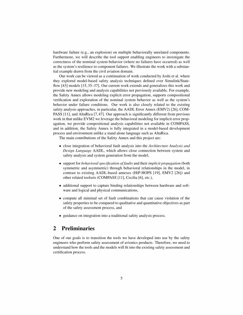
2.2 Modeling Language for System DesignFigure 1 presents our proposed use of a single unified model to support both systemdesign and safety analysis. It describes both system design and safety-relevant informa-tion that are kept distinguishable and yet are able to interact with each other. The sharedmodel is a living model that captures the current state of the system design as it movesthrough the development lifecycle, allowing all participants of the ARP4754A processto be able to communicate and review the system design. Safety analysis artifactscan be generated directly from the model, providing the capability to more accuratelyanalyze complex systems.
We are using the Architectural Analysis and Design Language (AADL) [25] toconstruct system architecture models. AADL is an SAE International standard that de-fines a language and provides a unifying framework for describing the system architec-ture for “performance-critical, embedded, real-time systems” [2]. From its conception,AADL has been designed for the design and construction of avionics systems. Ratherthan being merely descriptive, AADL models can be made specific enough to supportsystem-level code generation. Thus, results from analyses conducted, including thenew safety analysis proposed here, correspond to the system that will be built from themodel.
An AADL model describes a system in terms of a hierarchy of components and
6
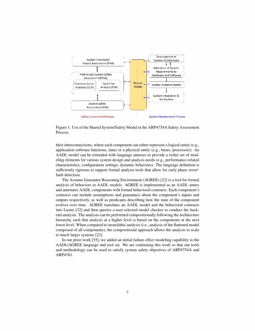
Figure 1: Use of the Shared System/Safety Model in the ARP4754A Safety AssessmentProcess
their interconnections, where each component can either represent a logical entity (e.g.,application software functions, data) or a physical entity (e.g., buses, processors). AnAADL model can be extended with language annexes to provide a richer set of mod-eling elements for various system design and analysis needs (e.g., performance-relatedcharacteristics, configuration settings, dynamic behaviors). The language definition issufficiently rigorous to support formal analysis tools that allow for early phase error/-fault detection.
The Assume Guarantee Reasoning Environment (AGREE) [22] is a tool for formalanalysis of behaviors in AADL models. AGREE is implemented as an AADL annexand annotates AADL components with formal behavioral contracts. Each component’scontracts can include assumptions and guarantees about the component’s inputs andoutputs respectively, as well as predicates describing how the state of the componentevolves over time. AGREE translates an AADL model and the behavioral contractsinto Lustre [32] and then queries a user-selected model checker to conduct the back-end analysis. The analysis can be performed compositionally following the architecturehierarchy such that analysis at a higher level is based on the components at the nextlower level. When compared to monolithic analysis (i.e., analysis of the flattened modelcomposed of all components), the compositional approach allows the analysis to scaleto much larger systems [22].
In our prior work [55], we added an initial failure effect modeling capability to theAADL/AGREE language and tool set. We are continuing this work so that our toolsand methodology can be used to satisfy system safety objectives of ARP4754A andARP4761.
7

2.3 Model-Based Safety Assessment Process Supported by FormalMethods
We propose a model-based safety assessment process backed by formal methods tohelp safety engineers with early detection of the design issues. This process uses asingle unified model to support both system design and safety analysis. It is based onthe following steps:
1. System engineers capture the critical information in a shared AADL/AGREEmodel: high-level hardware and software architecture, nominal behavior at thecomponent level, and safety requirements at the system level.
2. System engineers use the backend model checker to check that the safety re-quirements are satisfied by the nominal design model.
3. Safety engineers use the Safety Annex to augment the nominal model with thecomponent failure modes. In addition, safety engineers specify the fault hypoth-esis for the analysis which corresponds to how many simultaneous faults thesystem must be able to tolerate.
4. Safety engineers use the backend model checker to analyze if the safety require-ments and fault tolerance objectives are satisfied by the design in the presenceof faults. If the design does not tolerate the specified number of faults (or prob-ability threshold of fault occurrence), then the tool produces counterexamplesleading to safety requirement violation in the presence of faults, as well as allminimal set of fault combinations that can cause the safety requirement to beviolated.
5. The safety engineers examine the results to assess the validity of the fault com-binations and the fault tolerance level of the system design. If a design change iswarranted, the model will be updated with the latest design change and the aboveprocess is repeated.
There are other tools purpose-built for safety analysis, including AltaRica [47],smartIFlow [34] and xSAP [8]. These tools and their accompanying notations are sep-arate from the system development model. Other tools extend existing system models,such as HiP-HOPS [19] and the AADL Error Model Annex, Version 2 (EMV2) [26].EMV2 uses enumeration of faults in each component and explicit propagation of faultybehavior to perform error analysis. The required propagation relationships must bemanually added to the system model and can become complex, leading to mistakes inthe analysis.
In contrast, the Safety Annex supports model checking and quantitative reasoningby attaching behavioral faults to components and then using the normal behavioralpropagation and proof mechanisms built into the AGREE AADL annex. This allowsusers to reason about the evolution of faults over time, and produce counterexamplesdemonstrating how component faults lead to failures. Our approach adapts the workof Joshi et. al [37] to the AADL modeling language. Stewart, et. al provide moreinformation on the approach [55], and the tool and relevant documentation can be foundat: https://github.com/loonwerks/AMASE/.
8

2.4 Comparison with Proposed MBSA Appendix to ARP4761AARP4754A, the Guidelines for Development of Civil Aircraft and Systems [52],provides guidance on applying development assurance at each hierarchical levelthroughout the development life cycle of highly-integrated/complex aircraft systems.ARP4761, the Guidelines and Methods for Conducting Safety Assessment Process onCivil Airborne Systems and Equipment [51], identifies a systematic means to showcompliance. A Model Based Safety Analysis (MBSA) appendix has been drafted tothe upcoming revision of ARP4761 to provide concepts and processes with ModelBased Safety Analysis.
We have reviewed the draft appendix and found that our approach is consistent withthe MBSA appendix in the following ways:
• The common goal is to use MBSA for an equivalent analysis to the traditionalsafety analysis methods (e.g., Fault Trees) to support safety assessment pro-cesses.
• Both use an analytical model of the system to capture failure propagation. Inthe model, system architecture, nominal and faulty functional behaviors are cap-tured. The model evolves as the system design evolves.
• Both use software application/tools to perform analysis on the model and gener-ate outputs (e.g., failure sequences, minimal cut sets that result in the failure con-dition under analysis). The MBSA appendix also mentioned that model checkingcan be used to perform an exhaustive exploration of the state space of the model.
• Outputs generated from the analysis are to be compared to qualitative and/orquantitative objectives and requirements as part of the safety assessment process.Furthermore, the outputs drive evolution of system design.
Our approach goes beyond what is envisioned in the MBSA appendix in the fol-lowing ways:
• The MBSA Appendix is not advocating a single unified model used by both sys-tem development and safety assessment activities. The model is safety specificand driven by the types of safety assessment to be conducted. However, the ini-tial safety model may be derived from the system design model, and may becloser to the design at the lower levels of the design process.
• In the MBSA Appendix, the failure propagation modeling focuses on the insideinternal flows in the components, which is similar to the bottom-up method inFailure Modes and Effects Analysis. Different components are connected byinputs and outputs, and no behavioral constraints are specified on data enteringand exiting components. This leaves inter-component propagation to be exploredby the analysis.
In summary, our approach provides a new way to do safety analysis. It uses anunified model that is shared by system development and safety assessment. The model
9
captures architecture and behavioral information for propagation within componentsand between components. It is a property driven approach that is consistent betweensystem verification and safety analysis.
3 Fault Modeling with the Safety AnnexTo demonstrate the fault modeling capabilities of the Safety Annex we will use theWheel Brake System (WBS) described in AIR6110 [1]. This system is a well-knownexample that has been used as a case study for safety analysis, formal verification,and contract based design [10, 14, 15, 35]. The preliminary work for the safety annexwas based on a simple model of the WBS [55]. To demonstrate a more complex faultmodeling process, we constructed a functionally and structurally equivalent AADLversion of the more complex WBS NuSMV/xSAP models [15].
Figure 2: Wheel Brake System
The WBS is composed of two main parts: the Line Replaceable Unit control systemand the electro-mechanical physical system. The control system electronically controlsthe physical system and contains a redundant channel of the Braking System ControlUnit (BSCU) in case a detectable fault occurs in the active channel. It also commandsantiskid braking. The physical system consists of the hydraulic circuits running fromhydraulic pumps to wheel brakes as well as valves that control the hydraulic fluid flow.This system provides braking force to each of the eight wheels of the aircraft. Thewheels are all mechanically braked in pairs (one pair per landing gear). For simplicity,Figure 2 displays only two of the eight wheels.
There are three operating modes in the WBS model:
• In normal mode, the system is composed of a green hydraulic pump and onemeter valve per each of the eight wheels. Each of the meter valves are con-trolled through electronic commands coming from the active channel of the
10

BSCU. These signals provide braking and antiskid commands for each wheel.The braking command is determined through a sensor on the pedal and the anti-skid command is determined by the Wheel Sensors.
• In alternate mode, the system is composed of a blue hydraulic pump, four metervalves, and four antiskid shutoff valves, one for each landing gear. The metervalves are mechanically commanded through the pilot pedal corresponding toeach landing gear. If the selector detects lack of pressure in the green circuit, itswitches to the blue circuit.
• In emergency mode, the system mode is entered if the blue hydraulic pump fails.The accumulator pump has a reserve of pressurized hydraulic fluid and will sup-ply this to the blue circuit in emergency mode.
The WBS architecture model in AADL contains 30 different kinds of components,169 component instances, and a model depth of 5 hierarchical levels.
The behavioral model is encoded using the AGREE annex and the behavior is basedon descriptions found in AIR6110. The top level system properties are given by the re-quirements and safety objectives in AIR6110. All of the subcomponent contracts sup-port these system safety objectives through the use of assumptions on component inputand guarantees on the output. The WBS behavioral model in AGREE annex includesone top-level assumption and 11 top-level system properties, with 113 guarantees allo-cated to subsystems.
An example system safety property is to ensure that there is no inadvertent brakingof any of the wheels. This is based on a failure condition described in AIR6110 isInadvertent wheel braking on one wheel during takeoff shall be less than 1E-9 pertakeoff. Inadvertent braking means that braking force is applied at the wheel but thepilot has not pressed the brake pedal. In addition, the inadvertent braking requiresthat power and hydraulic pressure are both present, the plane is not stopped, and thewheel is rolling (not skidding). The property is stated in AGREE such that inadvertentbraking does not occur, as shown in Figure 3.
Figure 3: AGREE Contract for Top Level Property: Inadvertent Braking
3.1 Component Fault ModelingThe usage of the terms error, failure, and fault are defined in ARP4754A and are de-scribed here for ease of understanding [52]. An error is a mistake made in implementa-tion, design, or requirements. A fault is the manifestation of an error and a failure is anevent that occurs when the delivered service of a system deviates from correct behavior.If a fault is activated under the right circumstances, that fault can lead to a failure. The
11

terminology used in EMV2 differs slightly for an error: an error is a corrupted statecaused by a fault. The error propagates through a system and can manifest as a failure.In this report, we use the ARP4754A terminology with the added definition of errorpropagation as used in EMV2. An error is a mistake made in design or code and anerror propagation is the propagation of the corrupted state caused by an active fault.
The Safety Annex is used to add possible faulty behaviors to a component model.Within the AADL component instance model, an annex is added which contain the faultdefinitions for the given component. The flexibility of the fault definitions allows theuser to define numerous types of fault nodes by utilizing the AGREE node syntax. Alibrary of common fault nodes has been written and is available in the project GitHubrepository [53]. Examples of such faults include valves being stuck open or closed,output of a software component being nondeterministic, or power being cut off. Whenthe fault analysis requires fault definitions that are more complex, these nodes caneasily be written and used in the model.
When a fault is activated by its specified triggering conditions, it modifies the out-put of the component. This faulty behavior may violate the contracts of other compo-nents in the system, including assumptions of downstream components. The impact ofa fault is computed by the AGREE model checker when the safety analysis is run onthe fault model.
The majority of faults that are connected to outputs of components are known assymmetric. That is, whatever components receive this faulty output will receive thesame faulty output value. Thus, this output is seen symmetrically. An alternative faulttype is asymmetric. This pertains to a component with a 1-n output: one output whichis sent to many receiving components. This fault can present itself differently to thereceiving components. For instance, in a boolean setting, one component might see atrue value and the rest may see false. This is also possible to model using the keywordasymmetric. For more information on fault definitions and modeling possibilities, werefer readers to the Safety Annex Users Guide [53].
As an illustration of fault modeling using the Safety Annex, we look at one of thecomponents important to the inadvertent braking property: the brake pedal. When themechanical pedal is pressed, a sensor reads this information and passes an electronicsignal to the BSCU which then commands hydraulic pressure to the wheels.
Figure 4 shows the AADL pedal sensor component with a contract for its nominalbehavior. The sensor has only one input, the mechanical pedal position, and one output,the electrical pedal position. A property that governs the behavior of the component isthat the mechanical position should always equal the electronic position. (The expres-sion true→ property in AGREE is true in the initial state and then afterwards it is onlytrue if property holds.)
One possible failure for this sensor is inversion of its output value. This fault canbe triggered with probability 5.0× 10⁻⁶ as described in AIR6110 (in reality, the com-ponent failure probability is collected from hardware specification sheets). The SafetyAnnex definition for this fault is shown in Figure 5. Fault behavior is defined throughthe use of a fault node called inverted fail. When the fault is triggered, the nominal out-put of the component (elec pedal position) is replaced with its failure value (val out).
The WBS fault model expressed in the Safety Annex contains a total of 33 different
12

system SensorPedalPosition features -- Input ports for subcomponent
mech_pedal_pos : in data port Base_Types::Boolean; elec_pedal_pos : in data port Base_Types::Boolean;
-- Behavioral contracts for subcomponent annex agree {** guarantee "Mechanical and electrical pedal position is equivalent" : true -> (mech_pedal_position = elec_pedal_position; }; end SensorPedalPosition;
Figure 4: An AADL System Type: The Pedal Sensor
annex safety {** fault SensorPedalPosition_ErroneousData "Inverted boolean fault" : faults.inverted_fail { inputs: val_in <- elec_pedal_position;
outputs: elec_pedal_position <- val_out; probability: 5.0E-6 ; duration: permanent; } };
Figure 5: The Safety Annex for the Pedal Sensor
fault types and 141 fault instances. The large number of fault instances is due to theredundancy in the system design and its replication to control 8 wheels.
3.2 Implicit Error PropagationIn the Safety Annex approach, faults are captured as faulty behaviors that augment thesystem behavioral model in AGREE contracts. No explicit error propagation is neces-sary since the faulty behavior itself propagates through the system just as in the nominalsystem model. The effects of any triggered fault are manifested through analysis of theAGREE contracts.
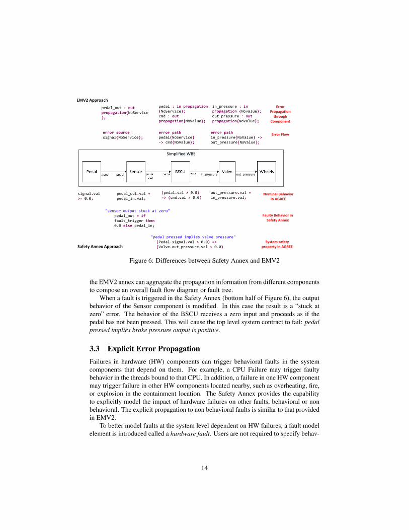
On the contrary, in the AADL Error Model Annex, Version 2 (EMV2) [26] ap-proach, all errors must be explicitly propagated through each component (by applyingfault types on each of the output ports) in order for a component to have an impact onthe rest of the system. To illustrate the key differences between implicit error propaga-tion provided in the Safety Annex and the explicit error propagation provided in EMV2,we use a simplified behavioral flow from the WBS example using code fragments fromEMV2, AGREE, and the Safety Annex.
In this simplified WBS system, the physical signal from the Pedal component isdetected by the Sensor and the pedal position value is passed to the Braking SystemControl Unit (BSCU) components. The BSCU generates a pressure command to theValve component which applies hydraulic brake pressure to the Wheels.
In the EMV2 approach (top half of Figure 6), the “NoService” fault is explicitlypropagated through all of the components. These fault types are essentially tokens thatdo not capture any analyzable behavior. At the system level, analysis tools supporting
13
Pedal BSCU Valve WheelsSensor
Safety Annex Approach
signal.val >= 0.0;
pedal_out.val = pedal_in.val;
signal pedal_in
pedal_out
pedal cmd
Simplified WBS
in_pressure out_pressure
pedal : in propagation {NoService};cmd : out propagation{NoValue};
in_pressure : in propagation {Novalue};out_pressure : out propagation{NoValue};
pedal_out : out propagation{NoService};
EMV2 Approach
Nominal Behavior in AGREE
Faulty Behavior in Safety Annex
Error Propagationthrough
Component
Error Flow
System safety property in AGREE
pedal_out = if fault_trigger then 0.0 else pedal_in;
error source signal{NoService};
error path pedal{NoService} ‐> cmd{NoValue};
error path in_pressure{NoValue} ‐> out_pressure{NoValue};
(pedal.val > 0.0) => (cmd.val > 0.0)
out_pressure.val = in_pressure.val;
(Pedal.signal.val > 0.0) => (Valve.out_pressure.val > 0.0)
"sensor output stuck at zero"
"pedal pressed implies valve pressure"
Figure 6: Differences between Safety Annex and EMV2
the EMV2 annex can aggregate the propagation information from different componentsto compose an overall fault flow diagram or fault tree.
When a fault is triggered in the Safety Annex (bottom half of Figure 6), the outputbehavior of the Sensor component is modified. In this case the result is a “stuck atzero” error. The behavior of the BSCU receives a zero input and proceeds as if thepedal has not been pressed. This will cause the top level system contract to fail: pedalpressed implies brake pressure output is positive.
3.3 Explicit Error PropagationFailures in hardware (HW) components can trigger behavioral faults in the systemcomponents that depend on them. For example, a CPU Failure may trigger faultybehavior in the threads bound to that CPU. In addition, a failure in one HW componentmay trigger failure in other HW components located nearby, such as overheating, fire,or explosion in the containment location. The Safety Annex provides the capabilityto explicitly model the impact of hardware failures on other faults, behavioral or nonbehavioral. The explicit propagation to non behavioral faults is similar to that providedin EMV2.
To better model faults at the system level dependent on HW failures, a fault modelelement is introduced called a hardware fault. Users are not required to specify behav-
14

ioral effects for the HW faults, nor are data ports necessary on which to apply the faultdefinition. An example of a model component fault declaration is shown below:
Users specify dependencies between the HW component faults and faults that aredefined in other components, either HW or SW. The hardware fault then acts as atrigger for dependent faults. This allows a simple propagation from the faulty HWcomponent to the SW components that rely on it, affecting the behavior on the outputsof the affected SW components.
In the WBS example, assume that both the green and blue hydraulic pumps arelocated in the same compartment in the aircraft and an explosion in this compartmentrendered both pumps inoperable. The HW fault definition can be modeled first in thegreen hydraulic pump component as shown in Figure 3.3. The activation of this faulttriggers the activation of related faults as seen in the propagate to statement shownbelow. Notice that these pumps need not be connected through a data port in order tospecify this propagation.
The fault dependencies are specified in the system implementation where the sys-tem configuration that causes the dependencies becomes clear (e.g., binding betweenSW and HW components, co-location of HW components).
3.4 Fault Analysis StatementsThe fault analysis statement (also referred to as the fault hypothesis) resides in theAADL system implementation that is selected for verification. This may specify eithera maximum number of faults that can be active at any point in execution:
or that the only faults to be considered are those whose probability of simultaneousoccurrence is above some probability threshold:
Tying back to the fault tree analysis in traditional safety analysis, the former is anal-ogous to restricting the cutsets to a specified maximum number of terms, and the latteris analogous to restricting the cutsets to only those whose probability is above someset value. In the former case, we assert that the sum of the true fault trigger variables
15

is at or below some integer threshold. In the latter, we determine all combinations offaults whose probabilities are above the specified probability threshold, and describethis as a proposition over fault trigger variables. With the introduction of dependentfaults, active faults are divided into two categories: independently active (activated byits own triggering event) and dependently active (activated when the faults they dependon become active). The top level fault hypothesis applies to independently active faults.Faulty behaviors augment nominal behaviors whenever their corresponding faults areactive (either independently active or dependently active).
4 Byzantine Fault ModelingA Byzantine or asymmetric fault is a fault that presents different symptoms to differ-ent observers [23]. In our modeling environment, asymmetric faults may be associatedwith a component that has a 1-n output to multiple other components. In this configura-tion, a symmetric fault will result in all destination components seeing the same faultyvalue from the source component. To capture the behavior of asymmetric faults (“dif-ferent symptoms to different observers”), it was necessary to extend our fault modelingmechanism in AADL.
4.1 Implementation of Asymmetric FaultsTo illustrate our implementation of asymmetric faults, assume a source component Ahas a 1-n output connected to four destination components (B-E) as shown in Figure 7under “Nominal System.” If a symmetric fault was present on this output, all fourconnected components would see the same faulty behavior. An asymmetric fault shouldbe able to present arbitrarily different values to the connected components.
To this end, “communication nodes” are inserted on each connection from compo-nent A to components B, C, D, and E (shown in Figure 7 under “Fault Model Archi-tecture.” From the users perspective, the asymmetric fault definition is associated withcomponent A’s output and the architecture of the model is unchanged from the nom-inal model architecture. Behind the scenes, these communication nodes are createdto facilitate potentially different fault activations on each of these connections. Thefault definition used on the output of component A will be inserted into each of thesecommunication nodes as shown by the red circles at the communication node output inFigure 7.
An asymmetric fault is defined for Component A as in Figure 8. This fault definesan asymmetric failure on Component A that when active, is stuck at a previous value(prev(Output, 0)). This can be interpreted as the following: some connected compo-nents may only see the previous value of Comp A output and others may see the correct(current) value when the fault is active. This fault definition is injected into the com-munication nodes and which of the connected components see an incorrect value iscompletely nondeterministic. Any number of the communication node faults (0. . . all)may be active upon activation of the main asymmetric fault.
16
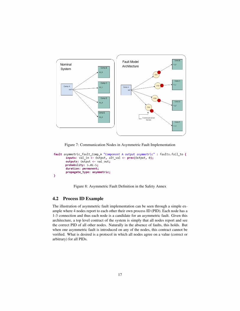
Figure 7: Communication Nodes in Asymmetric Fault Implementation
Figure 8: Asymmetric Fault Definition in the Safety Annex
4.2 Process ID ExampleThe illustration of asymmetric fault implementation can be seen through a simple ex-ample where 4 nodes report to each other their own process ID (PID). Each node has a1-3 connection and thus each node is a candidate for an asymmetric fault. Given thisarchitecture, a top level contract of the system is simply that all nodes report and seethe correct PID of all other nodes. Naturally in the absence of faults, this holds. Butwhen one asymmetric fault is introduced on any of the nodes, this contract cannot beverified. What is desired is a protocol in which all nodes agree on a value (correct orarbitrary) for all PIDs.
17
4.3 The Agreement Protocol Implementation in AGREEIn order to mitigate this problem, special attention must be given to the behavioralmodel. Using the strategies outlined in previous research [18, 23], the agreement pro-tocol is specified in AGREE to create a model resilient to one active Byzantine fault.
The objective of the agreement protocol is for all correct (non-failed) nodes toeventually reach agreement on the PID values of the other nodes. There are n nodes,possibly f failed nodes. The protocol requires n > 3f nodes to handle a single fault.The point is to achieve distributed agreement and coordinated decisions. The propertiesthat must be verified in order to prove the protocol works as desired are as follows:
• All correct (non-failed) nodes eventually reach a decision regarding the valuethey have been given. In this solution, nodes will agree in f + 1 time steps orrounds of communication.
• If the source node is correct, all other correct nodes agree on the value that wasoriginally sent by the source.
• If the source node is failed, all other nodes must agree on some predetermineddefault value.
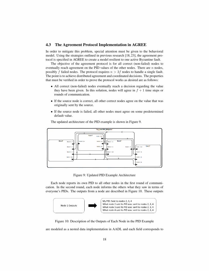
The updated architecture of the PID example is shown in Figure 9.
Figure 9: Updated PID Example Architecture
Each node reports its own PID to all other nodes in the first round of communi-cation. In the second round, each node informs the others what they saw in terms ofeveryone’s PIDs. The outputs from a node are described in Figure 10. These outputs
Figure 10: Description of the Outputs of Each Node in the PID Example
are modeled as a nested data implementation in AADL and each field corresponds to
18

a PID from a node. The AADL code fragment defining this data implementation isshown in Figure 11.
Figure 11: Data Implementation in AADL for Node Outputs
The fault definition for each node’s output and can effect the data fields arbitrarily.This is a nondeterministic fault in two ways. It is nondeterministic how many receivingnodes see incorrect values and it is nondeterministic how many of the data fields areaffected by this fault. This can be accomplished through the fault definition shown inFigure 12 and the fault node definition in Figure 13.
Figure 12: Fault Definition on Node Outputs for PID Example
Figure 13: Fault Node Definition for PID Example
19

Once the fault model is in place, the implementation in AGREE of the agreementprotocol is developed. As stated previously, there are two cases that must be consideredin the contracts of this system.
• In the case of no active faults, all nodes must agree on the correct PID of all othernodes.
• In the case of an active fault on a node, all non-failed nodes must agree on a PIDfor all other nodes.
These requirements are encoded in AGREE through the use of the following con-tracts. Figure 14 and Figure 15 show example contracts regarding Node 1 PID. Thereare similar contracts for each node’s PID.
Figure 14: Agreement Protocol Contract in AGREE for No Active Faults
Figure 15: Agreement Protocol Contract in AGREE Regarding Non-failed Nodes
Referencing Fault Activation Status To fully implement the agreement protocol,it must be possible to describe whether or not a subcomponent is failed by specifying ifany faults defined for the subcomponents is activated. In the Safety Annex, this is madepossible through the use of a fault activation statement. Users can declare boolean eqvariables in the AGREE annex of the AADL system where the AGREE verificationapplies to that system’s implementation. Users can then assign the activation status ofspecific faults to those eq variables in Safety Annex of the AADL system implementa-tion (the same place where the fault analysis statement resides). This assignment linkseach specified AGREE boolean variable with the activation status of the specified fault
20

activation literal. The AGREE boolean variable is true when and only when the fault isactive. An example of this for the PID example is shown in Figure 16. Each of the eqvariables declared in AGREE (i.e., n1 failed, n2 failed, n3 failed, n4 failed) is linkedto the fault activation status of the Asym Fail Any PID To Any Value fault defined in anode subcomponent instance of the AADL system implementation (i.e., node1, node2,node3, node4).
Figure 16: Fault Activation Statement in PID Example
4.4 PID Example Analysis ResultsThe nominal model verification shows that all properties are valid. Upon running verifi-cation of the fault model (Verify in the Presence of Faults) with one active fault, the firstfour properties stating that all nodes agree on the correct value (Figure 14) fail. Thisis expected since this property is specific to the case when no faults are present in themodel. The remaining 4 top level properties (Figure 15) state that all non-failed nodesreach agreement in two rounds of communication. These are verified valid when anyone asymmetric fault is present. This shows that the agreement protocol was success-ful in eliminating a single point of asymmetric failure from the model. Furthermore,when changing the number of allowed faults to two, these properties do not hold. Thisis expected given the theoretical result that 3f + 1 nodes are required in order to beresilient to f faults and that f + 1 rounds of communication are needed for successfulprotocol implementation. A summary of the results follows.
• Nominal model: All top level guarantees are verified. All nodes output the cor-rect value and all agree.
• Fault model with one active fault: The first four guarantees fail (when no faultis present, all nodes agree: shown in Figure 14). This is expected if faults arepresent. The last four guarantees (all non-failed nodes agree) are verified as truewith one active fault.
• Fault model with two active faults: All 8 guarantees fail. This is expected sincein order to be resilient up to two active faults (f = 2), we would need 3f+1 = 7nodes and f + 1 = 3 rounds of communication.
This model is in Github and is called PIDByzantineAgreement [53].
21

Figure 17: Safety Annex Plug-in Architecture
5 Tool Architecture and ImplementationThe Safety Annex is written in Java as a plug-in for the OSATE AADL toolset, whichis built on Eclipse. It is not designed as a stand-alone extension of the language, butworks with behavioral contracts specified using the AGREE AADL annex [22]. Thearchitecture of the Safety Annex is shown in Figure 17.
AGREE contracts are used to define the nominal behaviors of system componentsas guarantees that hold when assumptions about the values the component’s environ-ment are met. When an AADL model is annotated with AGREE contracts and the faultmodel is created using the Safety Annex, the model is transformed through AGREEinto a Lustre model [32] containing the behavioral extensions defined in the AGREEcontracts for each system component.
When performing fault analysis, the Safety Annex extends the AGREE contracts toallow faults to modify the behavior of component inputs and outputs. An example of aportion of an initial AGREE node and its extended contract is shown in Figure 18. Theleft column of the figure shows the nominal Lustre pump definition is shown with anAGREE contract on the output; and the right column shows the additional local vari-ables for the fault (boxes 1 and 2), the assertion binding the fault value to the nominalvalue (boxes 3 and 4), and the fault node definition (box 5). Once augmented with faultinformation, the AGREE model (translated into the Lustre dataflow language [32]) fol-lows the standard translation path to the model checker JKind [27], an infinite-statemodel checker for safety properties.
Figure 18: Nominal AGREE Node and Extension with Faults
22

There are two different types of fault analysis that can be performed on a faultmodel. The Safety Annex plugin intercepts the AGREE program and add fault modelinformation to the model depending on which form of fault analysis is being run.
Verification in the Presence of Faults: This analysis returns one counterexamplewhen fault activation per the fault hypothesis can cause violation of a property. Theaugmentation from Safety Annex to the AGREE program includes traceability infor-mation so that when counterexamples are displayed to users, the active faults for eachcomponent are visualized.
Generate Minimal Cut Sets: This analysis collects all minimal set of fault combi-nations that can cause violation of a property. Given a complex model, it is often usefulto extract traceability information related to the proof, in other words, which portionsof the model were necessary to construct the proof. An algorithm was introduced byGhassabani, et. al. to provide Inductive Validity Cores (IVCs) as a way to determinewhich model elements are necessary for the inductive proofs of the safety propertiesfor sequential systems [29]. Given a safety property of the system, a model checker canbe invoked in order to construct a proof of the property. The IVC generation algorithmextracts traceability information from the proof process and returns a minimal set ofthe model elements required in order to prove the property. Later research extendedthis algorithm in order to produce all Minimal Inductive Validity Cores (All-MIVCs)to provide a full enumeration of all minimal set of model elements necessary for theinductive proofs of a safety property [30].
In this approach, we use the all MIVCs algorithm to consider a constraint systemconsisting of the negation of the top level safety property, the contracts of system com-ponents, as well as the faults in each layer constrained to false. It then collects what arecalled Minimal Unsatisfiable Subsets (MUSs) of this constraint system; these are theminimal explanations of the constraint systems infeasibility in terms of the negationof the safety property. Equivalently, these are the minimal model elements necessaryto proof the safety property. In section 7.2, we show the formal definitions in detail.The leaf nodes contribute only constrained faults to the IVC elements as shown inFigure 19.
In the non-leaf layers of the program, both contracts and constrained faults areconsidered as shown in Figure 20. The reason for this is that the contracts are used toprove the properties at the next highest level and are necessary for the verification ofthe properties.
The all MIVCs algorithm returns the minimal set of these elements necessary toprove the properties. This equates to any contracts or inactive faults that must bepresent in order for the verification of properties in the model. From here, we performa number of algorithms to transform all MIVCs into minimal cut sets (see Section 7 formore details on the transformation algorithms).
6 Analysis of the ModelIn this section we describe results from the nominal model analysis and the fault anal-ysis.
23

Figure 19: IVC Elements used for Consideration in a Leaf Layer of a System
Figure 20: IVC Elements used for Consideration in a Middle Layer of a System
6.1 Nominal Model AnalysisBefore performing fault analysis, users should first check that the safety properties aresatisfied by the nominal design model. This analysis can be performed monolithicallyor compositionally in AGREE. Using monolithic analysis, the contracts at the lowerlevels of the architecture are flattened and used in the proof of the top level safetyproperties of the system. Compositional analysis, on the other hand, will perform theproof layer by layer top down, essentially breaking the larger proof into subsets ofsmaller problems. For a more comprehensive description of these types of proofs andanalyses, see additional publications related to AGREE [3, 21]
The WBS has a total of 13 safety properties at the top level that are supported bysubcomponent assumptions and guarantees. These are shown in Table 1. Given thatthere are 8 wheels, contract S18-WBS-0325-wheelX is repeated 8 times, one for eachwheel. The behavioral model in total consists of 36 assumptions and 246 supportingguarantees.
24

S18-WBS-R-0321Loss of all wheel braking during landing or RTO shall be less than 5.0× 10⁻⁷ per flight.
S18-WBS-R/L-0322Asymmetrical loss of wheel braking (Left/Right) shall be less than 5.0× 10⁻⁷ per flight.
S18-WBS-0323Never inadvertent braking with all wheels locked shall be less than 1.0× 10⁻⁹ per takeoff.
S18-WBS-0324Never inadvertent braking with all wheels shall be less than 1.0× 10⁻⁹ per takeoff.
S18-WBS-0325-wheelXNever inadvertent braking of wheel X shall be less than 1.0× 10⁻⁹ per takeoff. .
Table 1: Safety Properties of WBS
6.2 Fault Model AnalysisThere are two main options for fault model analysis using the Safety Annex. The firstoption injects faulty behavior allowed by faulty hypothesis into the AGREE model andreturns this model to JKind for analysis. This allows for the activity of faults within themodel and traceability information provides a way for users to view a counterexampleto a violated contract in the presence of faults. The second option is used to generateminimal cut sets for the model. The model is annotated with fault activation that areconstrained to false as well as intermediate level guarantees as model elements forconsideration for the all Minimal Inductive Validity Cores (All-MIVCs) algorithm. TheAll-MIVCs traces the minimal set of model elements used to produce minimal cut setsand is described in Section 7. This subsection presents these options and discusses theanalytical results obtained.
6.2.1 Verification in the Presence of Faults: Max N Analysis
Using a max number of faults for the hypothesis, the user can constrain the number ofsimultaneously active faults in the model. The faults are added to the AGREE modelfor the verification. Given the constraint on the number of possible simultaneouslyactive faults, the model checker attempts to prove the top level properties given theseconstraints. If this cannot be done, the counterexample provided will show which ofthe faults (N or less) are active and which contracts are violated.
The user can choose to perform either compositional or monolithic analysis usinga max N fault hypothesis. In compositional analysis, the analysis proceeds in a topdown fashion. To prove the top level properties, the properties in the layer directlybeneath the top level are used to perform the proof. The analysis proceeds in thismanner. Users constrain the maximum number of faults within each layer of the modelby specifying the maximum fault hypothesis statement to that layer. If any lower levelproperty failed due to activation of faults, the property verification at the higher levelcan no longer be trusted because the higher level properties were proved based on the
25

assumption that the direct sub-level contracts are valid. This form of analysis is helpfulto see weaknesses in a given layer of the system.
In monolithic analysis the layers of the model are flattened, which allows a directcorrespondence between all faults in the model and their effects on the top level prop-erties. As with compositional analysis, a counterexample shows these N or less activefaults.
6.2.2 Verification in the Presence of Faults: Probabilistic Analysis
Given a probabilistic fault hypothesis, this corresponds to performing analysis with thecombinations of faults whose occurrence probability is less than the probability thresh-old. This is done by inserting assertions that allow those combinations in the Lustrecode. If the model checker proves that the safety properties can be violated with any ofthose combinations, one of such combination will be shown in the counterexample.
Probabilistic analysis done in this way must utilize the monolithic AGREE option.For compositional probabilistic analysis, see Section 6.2.4.
To perform this analysis, it is assumed that the non-hardware faults occur inde-pendently and possible combinations of faults are computed and passed to the Lustremodel to be checked by the model checker. As seen in Algorithm 1, the computationfirst removes all faults from consideration that are too unlikely given the probabilitythreshold. The remaining faults are arranged in a priority queue Q from high to low.Assuming independence in the set of faults, we take a fault with highest probabilityfrom the queue (step 5) and attempt to combine the remainder of the faults in R (step7). If this combination is lower than the threshold (step 8), then we do not take intoconsideration this set of faults and instead remove the tail of the remaining faults inR.
Algorithm 1: Monolithic Probability Analysis
1 F = {} : fault combinations above threshold ;2 Q : faults, qi, arranged with probability high to low ;3 R = Q , with r ∈ R;4 while Q 6= {} ∧ R 6= {} do5 q = removeTopElement(Q) ;6 for i = 0 : |R| do7 prob = q × ri ;8 if prob < threshold then9 removeTail(R, j = i : |R|);
10 else11 add({q, ri},Q);12 add({q, ri},F);
In this calculation, we assume independence among the faults, but in the SafetyAnnex it is possible to define dependence between faults using a fault propagationstatement. After fault combinations are computed using Algorithm 1, the triggereddependent HW faults are added to the combination as appropriate. The dependenciesare implemented in the Verify in the Presence of Faults options for analysis, but not yetimplemented in the Generate Minimal Cut Sets analysis options.
26

6.2.3 Generate Minimal Cut Sets: Max N Analysis
As described in Section 5, Generate Minimal Cut Sets analysis uses the All-MIVCsalgorithm to provide a full enumeration of all minimal set of model elements necessaryfor the proof of each top-level safety property in the model, and then transforms allMIVCs into all minimal cut sets. In Max N analysis, the minimal cut sets are prunedto include only those with at cardinality less or equal to the max N number specified inthe fault hypothesis and displayed to the user.
Generate MinCutSet analysis was performed on the Wheel Brake System and re-sults are shown in Table 2. Notice in Table 2, the label across the top row refers to thecardinality (C) and how many cut sets of that cardinality. When the analysis is run, theuser specifies the value N. This gives cut sets of cardinality less than or equal to N.(For the full text of the properties, see Table 1.)
Property c = 1 c = 2 c = 3 c = 4 c = 5 c = 6 c = 7+
R-0321 6 0 0 1 144 7776 -R-0322 32 0 0 0 0 0 -L-0322 32 0 0 0 0 0 -0323 90 0 0 0 0 0 -0324 8 3,401 6,800 66,472 435,358 1,892,832 -0325-WX 20 0 0 0 0 0 -
Table 2: WBS MinCutSet Analysis Results for Cardinality c
Due to the increasing number of possible fault combinations at N = 6, the com-putational time increases quickly. The WBS analysis was only run to N = 6 for thisreason.
6.2.4 Generate Minimal Cut Sets: Probabilistic Analysis
Both probabilistic analysis and max N analysis use the same minimal cut set genera-tion algorithm, except that in probabilistic analysis, the minimal cut sets are pruned toinclude only those fault combinations whose probability of simultaneous occurrenceexceed the given threshold in the probability hypothesis. Note that with probablistichypothesis, Verify in the Presence of Faults is performed using only monolithic analy-sis, but generating minimal cut sets is performed using compositional analysis.
The probabilistic analysis for the WBS was given a top level threshold of 1.0×10⁻⁹as stated in AIR6110. The faults associated with various components were all givenprobability of occurrence compatible with the discussion in this same document.
As shown in Table 3, the number of allowable combinations drops considerablywhen given probabilistic threshold as compared to just fault combinations of certaincardinalities. For example, one contract (inadvertent wheel braking of all wheels) hadover a million minimal cut sets produced when looking at it in terms of max N analysis,
27
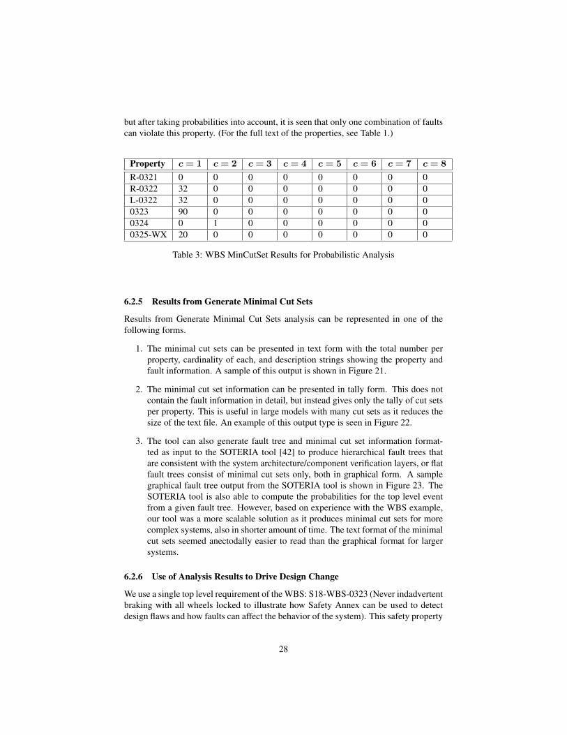
but after taking probabilities into account, it is seen that only one combination of faultscan violate this property. (For the full text of the properties, see Table 1.)
Property c = 1 c = 2 c = 3 c = 4 c = 5 c = 6 c = 7 c = 8
R-0321 0 0 0 0 0 0 0 0R-0322 32 0 0 0 0 0 0 0L-0322 32 0 0 0 0 0 0 00323 90 0 0 0 0 0 0 00324 0 1 0 0 0 0 0 00325-WX 20 0 0 0 0 0 0 0
Table 3: WBS MinCutSet Results for Probabilistic Analysis
6.2.5 Results from Generate Minimal Cut Sets
Results from Generate Minimal Cut Sets analysis can be represented in one of thefollowing forms.
1. The minimal cut sets can be presented in text form with the total number perproperty, cardinality of each, and description strings showing the property andfault information. A sample of this output is shown in Figure 21.
2. The minimal cut set information can be presented in tally form. This does notcontain the fault information in detail, but instead gives only the tally of cut setsper property. This is useful in large models with many cut sets as it reduces thesize of the text file. An example of this output type is seen in Figure 22.
3. The tool can also generate fault tree and minimal cut set information format-ted as input to the SOTERIA tool [42] to produce hierarchical fault trees thatare consistent with the system architecture/component verification layers, or flatfault trees consist of minimal cut sets only, both in graphical form. A samplegraphical fault tree output from the SOTERIA tool is shown in Figure 23. TheSOTERIA tool is also able to compute the probabilities for the top level eventfrom a given fault tree. However, based on experience with the WBS example,our tool was a more scalable solution as it produces minimal cut sets for morecomplex systems, also in shorter amount of time. The text format of the minimalcut sets seemed anectodally easier to read than the graphical format for largersystems.
6.2.6 Use of Analysis Results to Drive Design Change
We use a single top level requirement of the WBS: S18-WBS-0323 (Never indadvertentbraking with all wheels locked to illustrate how Safety Annex can be used to detectdesign flaws and how faults can affect the behavior of the system). This safety property
28
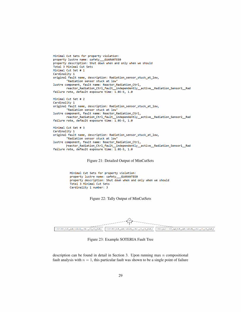
Figure 21: Detailed Output of MinCutSets
Figure 22: Tally Output of MinCutSets
Figure 23: Example SOTERIA Fault Tree
description can be found in detail in Section 3. Upon running max n compositionalfault analysis with n = 1, this particular fault was shown to be a single point of failure
29

for this safety property. A counterexample is shown in Figure 24 showing the activefault on the pedal sensor.
Figure 24: AGREE counterexample for inadvertent braking safety property
Depending on the goals of the system, the architecture currently modeled, and themitigation strategies that are desired, various strategies are possible to mitigate theproblem.
• Possible mitigation strategy 1: Monitor system can be added for the sensor: Amonitor sub-component can be modeled in which it accesses the mechanicalpedal as well as the signal from the sensor. If the monitor finds discrepanciesbetween these values, it can send an indication of invalid sensor value to the toplevel of the system. In terms of the modeling, this would require a change to thebehavioral contracts which use the sensor value. This validity would be takeninto account through the means of valid ∧ pedal sensor value.
• Possible mitigation strategy 2: Redundancy can be added to the sensor: A sensorsubsystem can be modeled which contains 3 or more sensors. The overall outputfrom the sensor system may utilize a voting scheme to determine validity ofsensor reading. There are multiple voting schemes that are possible, one of whichis a majority voting (e.g. one sensor fails, the other two take majority vote andthe correct value is passed). When three sensors are present, this mitigates thesingle point of failure problem. New behavioral contracts are added to the sensorsystem to model the behavior of redundancy and voting.
In the case of the pedal sensor in the WBS, the latter of the two strategies outlinedabove was implemented. A sensor system was added to the model which held threepedal sensors. The output of this subsystem was constrained using a majority votingscheme. Upon subsequent runs of the analysis (regardless which type of run was used),resilience was confirmed in the system regarding the failure of a single pedal sensor.Figure 25 outlines these architectural changes that were made in the model.
As can be seen through this single example, a system as large as the WBS wouldbenefit from many iterations of this process. Furthermore, if the model is changed
30

Figure 25: Changes in the architectural model for fault mitigation
even slightly on the system development side, it would automatically be seen from thesafety analysis perspective and any negative outcomes would be shown upon subse-quent analysis runs. This effectively eliminates any miscommunications between thesystem development and analysis teams and creates a new safeguard regarding modelchanges.
For more information on types of fault models that can be created as well as detailson analysis results, see the users guide located in the GitHub repository [53]. Thisrepository also contains all models used in this project.
7 Theoretical FoundationsThere are two different types of fault analysis that can be performed on a fault model,Verification in the Presence of Faults, and Generate Minimal Cut Sets, as introduced inSection 5. The theoretical foundations used to verify a model in the presence of faultsrelies on AGREE and the theory underlying the assume guarantee environment [21];this theory will not be discussed further in this report. The underlying theoreticalframework used in the generation of minimal cut sets is described in detail in thissection.
7.1 Fault Tree AnalysisThe use of fault trees are common in many safety assessment processes and the abilityto generate the cut sets needed for the construction of the fault tree is a useful partof any safety analysis tool. The fault tree is a safety artifact commonly referenced inrequirement protocol documents such as ARP4761, ARP4754, and AIR6110 [1,51,52].
A Fault Tree (FT) is a directed acyclic graph whose leaves model component fail-ures and whose gates model failure propagation [50]. The system failure under exami-nation is the root of the tree and is called the Top Level Event (TLE). The node types ina fault tree are events and gates. An event is an occurrence within the system, typicallythe failure of a subsystem down to an individual component. Events can be groupedinto Basic Events (BEs), which occur independently, and intermediate events which oc-cur dependently and are caused by one or more other events [24]. These events model
31

the failure of the system (or subsystem) under consideration. The gates represent howfailures propagate through the system and how failures in subsystems can cause systemwide failures. The two main logic symbols used are the Boolean logic AND-gates andOR-gates. An AND-gate is used when the undesired top level event can only occurwhen all the lower conditions are true. The OR-gate is used when the undesired eventcan occur if any one or more of the next lower conditions is true. This is not a compre-hensive list of gate types, but we focus our attention on these two common gate types.
Loss ofall
WheelBraking
Loss of NormalBraking
Loss of AlternateBraking
Loss of ReserveBraking
Figure 26: A simple fault tree
Figure 26 shows a simple example of a fault tree based on SAE ARP4761 [51]. Inthis example, the top level event corresponds to an aircraft losing all wheel braking. Inorder for this event to occur, all of the basic events must occur. This is seen throughthe use of the AND gate below the top level event. The gates in the fault tree describehow failures propagate through the system. Each gate has one output and one or moreinputs. In Figure 26, the AND gate has three inputs and one output. The leaves ofthe tree represent the basic events of the system. In the case of this fault tree, thesethree events are also the Minimal Cut Sets (MinCutSets) for this top level event. AMinCutSet is the minimal set of basic events that must occur together in order to causethe TLE to occur. Generating and analyzing these MinCutSets is important to FTA andhas been an active area of interest in the research community since fault trees were firstdescribed in Bell Labs in 1961 [24, 50].
There are two main types of fault tree analysis that we differentiate here as qual-itative analysis and quantitative analysis. In qualitative analysis, the structure of thefault tree is considered and the MinCutSets are a way to indicate which combinationsof component failures will cause the system to fail. On the other hand, in quantitativeanalysis the probability of the TLE is calculated given the probability of occurrence ofthe basic events. By being able to generate MinCutSets based on both cardinality andprobability, this allows for either form of FTA to be created.
32

7.2 DefinitionsIntuitively a constraint system contains the contracts that constrain component behaviorand faults that are defined over these components. In the case of a nominal modelaugmented with faults, a constraint system is defined as follows. Let F be the set of allfault activation literals defined in the model andG be the set of all component contracts(guarantees).
Definition 1. A constraint system C = {C1, C2, ..., Cn} where for i ∈ {1, ..., n}, Cihas the following constraints for any fj ∈ F and gk ∈ G with regard to the top levelproperty P :
Ci ∈
fj : inactivegk : trueP : false
Given a state space S, a transition system (I, T ) consists of the initial state predi-cate I : S → {0, 1} and a transition step predicate T : S × S → {0, 1}. Reachabilityfor (I, T ) is defined as the smallest predicate R : S → {0, 1} that satisfies the follow-ing formulas:
∀s.I(s)⇒ R(s)∀s, s′.R ∧ T (s, s′)⇒ R(s′)
A safety property P : S → {0, 1} is a state predicate. A safety property P holds on atransition system (I, T ) if it holds on all reachable states. More formally, ∀s.R(s) ⇒P(s). When this is the case, we write (I, T ) ` P [30].
Given a transition system that satisfies a safety property P , it is possible to findwhich model elements are necessary for satisfying the safety property through the useof the All Minimal Inductive Validity Cores All-MIVCs algorithms [4, 30]. This algo-rithm collects all minimal unsatisfiable subsets of a given transition system in termsof the negation of the top level property. The minimal unsatisfiable subsets consistof component contracts constrained to true. When the constraints on these model el-ements are removed from the constraint system C, this results in an UNSAT system.This can be seen as the minimal explanation of the constraint systems infeasibility. Re-call that this constraint system is in terms of the negation of the safety property. Thus,this algorithm provides all model elements required for the proof of the safety property.
We utilize this algorithm by providing not only component contracts (constrainedto true) as model elements, but also fault activation literals constrained to false. Thusthe resulting MIVCs will contain the required contracts and constrained fault activationliterals in order to prove the safety property. This information is used throughout thissection to provide the underlying theory behind the generation of minimal cut sets fromall MIVCs.
Definitions 1-3 are taken from research by Liffiton et. al. [40].
Definition 2. : A Minimal Unsatisfiable Subset (MUS) of a constraint system C is :{MUS ⊆ C | MUS is UNSAT and ∀c ∈ MUS: MUS \ {c} is SAT}. This is theminimal explaination of the constraint systems infeasability.
33

A closely related set is a minimal correction set (MCS). The MCSs describe theminimal set of model elements for which if constraints are removed, the constraintsystem is satisfied. For constraint system C, this corresponds to which faults are notconstrained to inactive (and are hence active) and violated contracts which lead to theviolation of the safety property. In other words, the minimal set of active faults and/orviolated properties that lead to the top level event.
Definition 3. : A Minimal Correction Set (MCS) of a constraint system C is :{MCS ⊆ C | C \MCS is SAT and ∀S ⊂MCS : C \ S is UNSAT}. A MCS can beseen to “correct” the infeasability of the constraint system.
A duality exists between MUSs of a constraint system and MCSs as established byReiter [49]. This duality is defined in terms of minimal hitting sets. A hitting set of acollection of setsA is a setH such that every set inA is “hit” beH; H contains at leastone element from every set in A [40]. The MCSs can be generated from the MUSs ifall MUSs are known. Thus, the use of the All-MIVCs algorithm is required.
Definition 4. : Given a collection of sets K, a hitting set for K is a set H ⊆ ∪S∈KSsuch that H ∩ S 6= ∅ for each S ∈ K. A hitting set for K is minimal if and only if noproper subset of it is a hitting set for K.
Utilizing this approach, the MCSs are generated from the MUSs that are providedby the All-MIVCs algorithm [30] and a minimal hitting set algorithm developed byMurakami et. al. [28, 45].
A Minimal Cut Set (MinCutSet) is a minimal collection of faults that lead to theviolation of the safety property (or in other words, lead to the top level event in thefault tree). We define a minimal cut set consistently with much of the research in thisfield [24, 50]
Definition 5. : A Minimal Cut Set can be defined as the set of faults in a system thatcause the violation of the safety property. Furthermore, any strict subset of these faultswill not cause violation of the safety property.
7.3 Transformation of All-MIVCs into Minimal Cut SetsAll Minimal Inductive Validity Cores are collected by use of the All-MIVCs algo-rithm [30]. These are all of the Minimal Unsatisfiable Subsets (MUSs) which can beused as input to the Minimal Hitting Set algorithm [28, 45] in order to collect all Min-imal Correction Sets (MCSs). The MCSs are then transformed into Minimal Cut Setsaccording to the following theoretical results.
The definition of the constraint system follows Definition 1 in Section 7.2.
Theorem 1. The MinCutSet can be generated by the transformation of the MinimalCorrection Set (MCS).
Proof. All MCSs are of the form MCS = G ∪ F where G consists of contracts inthe system and F consists of faults constrained to false for constraint system C.
34

Case 1: G = ∅In the leaf level of the system, only constrained faults are contained in MCS. Accord-ing to the defintion of an MCS, upon removing the constraints from C of the elementscontained in the MCS, the constraint system is satisfiable. Furthermore, the MCS isthe minimal such set. Thus, the constraint system with the active faults from MCSwill cause the negation of the safety property to be satisfied. The set of unconstrainedfaults found in the MCS is the defintion of a minimal cut set.
Case 2: G 6= ∅Let MCS = {¬f1, ...,¬fn, g1, ..., gm} where fj ∈ F and gk ∈ G and ¬f is a faultactivation literal f constrained to false. For all gi ∈ MCS, we know that the validityof gk is required in the proof of the top level property P due to its generation throughthe All-MIVCs algorithm. For g1 ∈ MCS, there exists a set containing all minimalcut sets of g1. Call this Cut(g1) = {F1i ⊆ F |F1i is a min cut set for g1, i = 1, ..., p1}.
Replace g1 with F1i for all i = 1, ..., p1. This produces p1 new MCSs of the form:
{f1, ..., fn, F11, ..., gm}{f1, ..., fn, F12, ..., gm}
...{f1, ..., fn, F1p1 , ..., gm}
Perform this replacement for all gk ∈MCS, k = 1, ...,m.Let Iα be one of the sets generated by full replacement of all contracts in
some MCSα with their respective minimal cut set and all fault activation literalsconstrainted to true.
Claim: Iα is a minimal cut set for safety property PBy the definition of MCSα, C \MCSα is SAT. Thus the fault activation literals inMCSα are true and the contracts in MCSα are violated. This combination will causeviolation of the safety property (i.e., the constraint system C \MCSα is SAT).
The generation of Iα consists of replacing all contracts in MCSα by theirrespective minimal cut sets and unconstraining all fault activation literals in MCSα.These unconstrained faults cause the violation of all contracts in MCSα. Hencetogether, the violation of P since C \MCSα is SAT. Therefore Iα is a cut set for P .
Minimality follows from the defintion of MCS:
Assume that Iβ ⊂ Iα. Then there is at least one f ∈ Iα where f 6∈ Iβ . Let ¬f bethe fault activation literal f constrained to false.
If ¬f ∈ MCSα and f 6∈ Iβ , then by removing all constraints of the fault literalsin Iβ from C (C \ Iβ), we see that the resulting constraint system is UNSAT by theminimality of MCSα. Therefore Iβ is not a cut set for P .
If f ∈ MinCut(g) where MinCut(g) is a minimal cut set for some g ∈ MCSα,then C \ Iβ will not remove constraints for all of the elements in MinCut(g) andtherefore g remains unviolated, i.e., the constraint that g is true is not removed. Thus
35

C\Iβ will not remove constraints for all of the elements inMCSα which meansC\Iβis UNSAT. Therefore Iβ is not a cut set for P .
The generation of MIVCs traverses the program in a top down fashion. The trans-formation of MIVCs to MinCutSets traverses this tree in a bottom up fashion if andonly if All-MIVCs have been generated. It is a requirement of the minimal hitting setalgorithm that all MUSs are used to find the MCSs [28,40,45]. Thus, once All-MIVCshave been found and the minimal hitting set algorithm has completed, the MinCutSetsGeneration algorithm can begin.
The MinCutSets Generation Algorithm begins with a list of MCSs specific to atop level property. These MCSs may contain a mixture of fault activation literals con-strained to false and and subcomponent contracts constrained to true. We remove allconstraints from each MCS and call the resulting sets I , for Intermediate set. Re-placement of subcomponent contracts with their respective minimal cut sets can thenproceed. For each of those contracts in I , we check to see if we have previously ob-tained a MinCutSet for that contract. If so, replacement is performed. If not, werecursively call this algorithm to obtain the list of all MinCutSets associated with thissubcomponent contract. At a certain point, there will be no more contracts in the set Iin which case we have a minimal cut set for the current property. When this set is ob-tained, we store it in a lookup table keyed by the given property that this I is associatedwith.
Notes regarding the following algorithm: at the onset, the current property P is atop level property. Each of the properties has a list of associated MCSs. When thealgorithm states that constraints on these elements are removed, more specifically thefault activation literals in MCS are constrained to true and the component contractsare constrained to false. List(I) is the collection of all MCSs with all constraintsremoved. Assuming All-MIVCs have been found and the minimal hitting set algorithmhas terminated, giving us a list of MCSs for each property in the system.
36
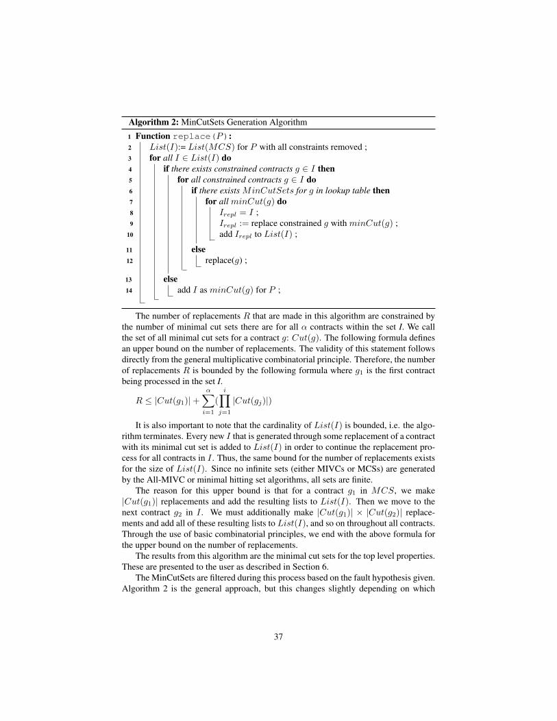
Algorithm 2: MinCutSets Generation Algorithm
1 Function replace(P):2 List(I):= List(MCS) for P with all constraints removed ;3 for all I ∈ List(I) do4 if there exists constrained contracts g ∈ I then5 for all constrained contracts g ∈ I do6 if there exists MinCutSets for g in lookup table then7 for all minCut(g) do8 Irepl = I ;9 Irepl := replace constrained g with minCut(g) ;
10 add Irepl to List(I) ;
11 else12 replace(g) ;
13 else14 add I as minCut(g) for P ;
The number of replacements R that are made in this algorithm are constrained bythe number of minimal cut sets there are for all α contracts within the set I. We callthe set of all minimal cut sets for a contract g: Cut(g). The following formula definesan upper bound on the number of replacements. The validity of this statement followsdirectly from the general multiplicative combinatorial principle. Therefore, the numberof replacements R is bounded by the following formula where g1 is the first contractbeing processed in the set I.
R ≤ |Cut(g1)|+α∑i=1
(
i∏j=1
|Cut(gj)|)
It is also important to note that the cardinality of List(I) is bounded, i.e. the algo-rithm terminates. Every new I that is generated through some replacement of a contractwith its minimal cut set is added to List(I) in order to continue the replacement pro-cess for all contracts in I . Thus, the same bound for the number of replacements existsfor the size of List(I). Since no infinite sets (either MIVCs or MCSs) are generatedby the All-MIVC or minimal hitting set algorithms, all sets are finite.
The reason for this upper bound is that for a contract g1 in MCS, we make|Cut(g1)| replacements and add the resulting lists to List(I). Then we move to thenext contract g2 in I . We must additionally make |Cut(g1)| × |Cut(g2)| replace-ments and add all of these resulting lists to List(I), and so on throughout all contracts.Through the use of basic combinatorial principles, we end with the above formula forthe upper bound on the number of replacements.
The results from this algorithm are the minimal cut sets for the top level properties.These are presented to the user as described in Section 6.
The MinCutSets are filtered during this process based on the fault hypothesis given.Algorithm 2 is the general approach, but this changes slightly depending on which
37

form of analysis is being performed. These differences are outlined in the followingsubsections.
7.3.1 Transformation Algorithm for Max N Analysis
Given a top level fault hypothesis statement of maximum N faults, the transformationalgorithm filters out any MinCutSets of cardinality greater than N . To assist in per-formance and scalability, if a minimum cut set exceeds the cardinality of N , it will nolonger be considered for the algorithm. We call this pruning. This pruning is done inAlgorithm 2 in Section 7.3. If the number of faults in an intermediate set I exceedsN , any further replacement of remaining contracts in that intermediate set can neverdecrease the total number of faults in I . Only the remaining sets are displayed.
7.3.2 Probabilistic Analysis Algorithm
In order to complete the probabilistic analysis, we must first calculate allowable com-binations of faults. This allows us the option to eliminate unnecessary combinationswhile performing the algorithm, thus increasing performance and diminishing the prob-lem of combinatorial explosions in the size of minimal cut sets for larger models.
After the allowable combinations have been found, the algorithm described inSection 7.3 is performed with pruning in order to eliminate probabilistically impossiblefault combinations.
Collect Allowable Fault Combinations The collection of allowable fault combi-nations is a prerequsite needed for both Verify in the Presence of Faults and GenerateMinimal Cut Set analysis and the algorithm used is described in Section 6.2.2. In or-der to calculate allowable combinations, we must take into account probabilities of thecombined faults and compare with the given threshold. Each of the allowable faultcombinations has a combined probability that we must later access. These combina-tions are saved in a list called A:A = {Ai = FaultCombinations | P (FaultCombinations) > threshold}The allowable combinations in A consist of independent faults.
Prune MinCutSets During the transformation process, if the minimal cut set for acontract is not a subset of any allowed fault combinations, this intermediate set contain-ing this contract is pruned. (Recall that an intermediate set I is obtained by removingall constraints from an MCS and contract replacement has begun.) This pruning oc-curs in the algorithm described in Section 7.3 and the resulting allowable combinationsare displayed to the user.
The implementation of the Safety Annex utilizes the pruning as described above.Theoretically, there are two other options for pruning in this algorithm. They are out-lined here for completion. Throughout this discussion, we use the following notationto describe these sets. They are listed here for convenience.A : the set of all allowable fault combinationsAi : an individual allowable combination and an element of AList(I) : the set of all intermediate sets
38

Ii : an element of List(I).Cut(gj) : all minimal cut sets for contract gj .cutk(gj) : a specific cut set for contract gj . This is an element of Cut(gj).
Option 1: Once the replacement is complete and the algorithm terminates, wehave all MinCutSets for a top level property. If MinCutSet 6⊆ Ai for all Ai ∈ A,then we can safely eliminate MinCutSet. This is the latest form of pruning and thedrawback is when the number of generated cut sets grows, no elimination occurs early.This can be difficult in terms of scalability.
Option 2: Pruning can also be done by checking the union of a minimal cut setfor a contract in I with all the faults in that I . If the union of these faults is not anallowable combination, the minimal cut set for this contract in I will be skipped for thereplacement. More formally, if ({fn|fn ∈ Ii} ∪ cutk(gj)) 6⊆ Ai for all Ai ∈ A, thenwe can safely eliminate this Ii.
8 Related WorkA model-based approach for safety analysis was proposed by Joshi et. al in [35–37].In this approach, a safety analysis system model (SASM) is the central artifact in thesafety analysis process, and traditional safety analysis artifacts, such as fault trees, areautomatically generated by tools that analyze the SASM.
The contents and structure of the SASM differ significantly across different concep-tions of MBSA. We can draw distinctions between approaches along several differentaxes. The first is whether they propagate faults explicitly through user-defined prop-agations, which we call failure logic modeling (FLM) or through existing behavioralmodeling, which we call failure effect modeling (FEM). The next is whether modelsand notations are purpose-built for safety analysis vs. those that extend existing systemmodels (ESM).
For FEM approaches, there are several additional dimensions. One dimension in-volves whether causal or non-causal models are allowed. Non-causal models allowsimultaneous (in time) bi-directional error propagations, which allow more natural ex-pression of some failure types (e.g. reverse flow within segments of a pipe), but aremore difficult to analyze. A final dimension involves whether analysis is composi-tional across layers of hierarchically-composed systems or monolithic. Our approachis an extension of AADL (ESM), causal, compositional, mixed FLM/FEM approach.
Tools such as the AADL Error Model Annex, Version 2 (EMV2) [26] and HiP-HOPS for EAST-ADL [19] are FLM-based ESM approaches. As previously discussed,given many possible faults, these propagation relationships require substantial user ef-fort and become more complex. In addition, it becomes the analyst’s responsibility todetermine whether faults can propagate; missing propagations lead to unsound analy-ses. In our Safety Annex, propagations occur through system behaviors (defined by thenominal contracts) with no additional user effort.
Closely related to our work is the model-based safety assessment toolset calledCOMPASS (Correctness, Modeling project and Performance of Aerospace Sys-tems) [11]. COMPASS is a mixed FLM/FEM-based, causal compositional tool suite
39
that uses the SLIM language, which is based on a subset of AADL, for its input mod-els [12, 16]. In SLIM, a nominal system model and the error model are developedseparately and then transformed into an extended system model. This extended modelis automatically translated into input models for the NuSMV model checker [20, 46],MRMC (Markov Reward Model Checker) [38, 44], and RAT (Requirements AnalysisTool) [48]. The safety analysis tool xSAP [8] can be invoked in order to generate safetyanalysis artifacts such as fault trees and FMEA tables [9]. COMPASS is an impressivetool suite, but some of the features that make AADL suitable for SW/HW architecturespecification: event and event-data ports, threads, and processes, appear to be missing,which means that the SLIM language may not be suitable as a general system designnotation (ESM).
SmartIFlow [34] is a FEM-based, purpose-built, monolithic non-causal safety anal-ysis tool that describes components and their interactions using finite state machinesand events. Verification is done through an explicit state model checker which returnssets of counterexamples for safety requirements in the presence of failures. SmartI-Flow allows non-causal models containing simultaneous (in time) bi-directional errorpropagations. On the other hand, the tools do not yet appear to scale to industrial-sizedproblems, as mentioned by the authors [34]: “As current experience is based on mod-els with limited size, there is still a long way to go to make this approach ready forapplication in an industrial context”.
The Safety Analysis and Modeling Language (SAML) [31] is a FEM-based,purpose-built, monolithic causal safety analysis language. System models constructedin SAML can be used used for both qualitative and quantitative analyses. It allows forthe combination of discrete probability distributions and non-determinism. The SAMLmodel can be automatically imported into several analysis tools like NuSMV [20],PRISM (Probabilistic Symbolic Model Checker) [39], or the MRMC probabilisticmodel checker [38].
AltaRica [7,47] is a FEM-based, purpose-built, monolithic safety analysis languagewith several dialects. There is one dialect of AltaRica which use dataflow (causal)semantics, while the most recent language update (AltaRica 3.0) uses non-causal se-mantics. The dataflow dialect has substantial tool support, including the commercialCecilia OCAS tool from Dassault [6]. For this dialect the Safety assessment, fault treegeneration, and functional verification can be performed with the aid of NuSMV modelchecking [13]. Failure states are defined throughout the system and flow variables areupdated through the use of assertions [5]. AltaRica 3.0 has support for simulation andMarkov model generation through the OpenAltaRica (www.openaltarica.fr) tool suite.
Formal verification tools based on model checking have been used to automatethe generation of safety artifacts [8, 13, 17]. This approach has limitations in terms ofscalability and readability of the fault trees generated. Work has been done towardsmitigating these limitations by the scalable generation of readable fault trees [14].
9 ConclusionWe have developed an extension to the AADL language with tool support for for-mal analysis of system safety properties in the presence of faults. Faulty behavior is
40

specified as an extension of the nominal model, allowing safety analysis and systemimplementation to be driven from a single common model. Both symmetric and asym-metric faulty behaviors are supported. This new Safety Annex leverages the AADLstructural model and nominal behavioral specification (using the AGREE annex) topropagate faulty component behaviors without the need to add separate propagationspecifications to the model. Implicit error propagation enables safety engineers to in-ject failures/faults at component level and assess the effect of behavioral propagation atthe system level. It also supports explicit error propagation that allows safety engineersto describe dependent faults that are not easily captured using implicit error propaga-tion. Generation of minimal cut sets collects all minimal set of fault combinations thatcan cause violation of the top level properties. For more details on the tool, models,and approach, see the technical report [54]. To access the tool plugin, users manual, ormodels, see the repository [53].
Acknowledgments. This research was funded by NASA contract NNL16AB07T andthe University of Minnesota College of Science and Engineering Graduate Fellowship.
References[1] AIR 6110. Contiguous Aircraft/System Development Process Example, Dec.
2011.
[2] AS5506C. Architecture Analysis & Design Language (AADL), Jan. 2017.
[3] J. Backes, D. Cofer, S. Miller, and M. W. Whalen. Requirements Analysis of aQuad-Redundant Flight Control System. In NFM, volume 9058 of LNCS, pages82–96, 2015.
[4] J. Bendık, E. Ghassabani, M. Whalen, and I. Cerna. Online enumeration of allminimal inductive validity cores. In International Conference on Software Engi-neering and Formal Methods, pages 189–204. Springer, 2018.
[5] P. Bieber, C. Bougnol, C. Castel, J. P. Heckmann, C. Kehren, S. Metge, andC. Seguin. Safety Assessment with Altarica - Lessons Learnt Based on TwoAircraft System Studies. In In 18th IFIP World Computer Congress, 2004.
[6] P. Bieber, C. Bougnol, C. Castel, J.-P. H. C. Kehren, S. Metge, and C. Seguin.Safety assessment with altarica. In Building the Information Society, pages 505–510. Springer, 2004.
[7] P. Bieber, J.-L. Farges, X. Pucel, L.-M. Sejeau, and C. Seguin. Model - basedsafety analysis for co-assessment of operation and system safety: application tospecific operations of unmanned aircraft. In ERTS2, 2018.
[8] B. Bittner, M. Bozzano, R. Cavada, A. Cimatti, M. Gario, A. Griggio, C. Mattarei,A. Micheli, and G. Zampedri. The xSAP Safety Analysis Platform. In TACAS,2016.
[9] M. Bozzano, H. Bruintjes, A. Cimatti, J.-P. Katoen, T. Noll, and S. Tonetta. Thecompass 3.0 toolset (short paper). In IMBSA 2017, 2017.
41

[10] M. Bozzano, A. Cimatti, A. Griggio, and C. Mattarei. Efficient Anytime Tech-niques for Model-Based Safety Analysis. In Computer Aided Verification, 2015.
[11] M. Bozzano, A. Cimatti, J.-P. Katoen, V. Y. Nguyen, T. Noll, and M. Roveri. TheCOMPASS Approach: Correctness, Modelling and Performability of AerospaceSystems. In Computer Safety, Reliability, and Security. Springer Berlin Heidel-berg, 2009.
[12] M. Bozzano, A. Cimatti, J.-P. Katoen, V. Yen Nguyen, T. Noll, and M. Roveri.Model-based codesign of critical embedded systems. 507, 2009.
[13] M. Bozzano, A. Cimatti, O. Lisagor, C. Mattarei, S. Mover, M. Roveri, andS. Tonetta. Symbolic Model Checking and Safety Assessment of Altarica Models.In Science of Computer Programming, volume 98, 2011.
[14] M. Bozzano, A. Cimatti, C. Mattarei, and S. Tonetta. Formal safety assessmentvia contract-based design. In Automated Technology for Verification and Analysis,2014.
[15] M. Bozzano, A. Cimatti, A. F. Pires, D. Jones, G. Kimberly, T. Petri, R. Robinson,and S. Tonetta. Formal Design and Safety Analysis of AIR6110 Wheel BrakeSystem. In CAV 2015, Proceedings, Part I, pages 518–535, 2015.
[16] M. Bozzano, A. Cimatti, M. Roveri, J. P. Katoen, V. Y. Nguyen, and T. Noll.Codesign of dependable systems: A component-based modeling language. In2009 7th IEEE/ACM International Conference on Formal Methods and Modelsfor Co-Design, 2009.
[17] M. Bozzano, A. Cimatti, and F. Tapparo. Symbolic fault tree analysis for reactivesystems. In ATVA, 2007.
[18] G. Bracha. Asynchronous byzantine agreement protocols. Information and Com-putation, 75(2):130–143, 1987.
[19] D. Chen, N. Mahmud, M. Walker, L. Feng, H. Lonn, and Y. Papadopoulos. Sys-tems Modeling with EAST-ADL for Fault Tree Analysis through HiP-HOPS*.IFAC Proceedings Volumes, 46(22):91 – 96, 2013.
[20] A. Cimatti, E. Clarke, F. Giunchiglia, and M. Roveri. Nusmv: a new symbolicmodel checker. International Journal on Software Tools for Technology Transfer,2000.
[21] D. Cofer, A. Gacek, S. Miller, M. W. Whalen, B. LaValley, and L. Sha. Composi-tional verification of architectural models. In NASA Formal Methods Symposium,pages 126–140. Springer, 2012.
[22] D. D. Cofer, A. Gacek, S. P. Miller, M. W. Whalen, B. LaValley, and L. Sha.Compositional Verification of Architectural Models. In NFM 2012, volume 7226,pages 126–140, April 2012.
42

[23] K. Driscoll, H. Sivencrona, and P. Zumsteg. Byzantine Fault Tolerance, fromTheory to Reality. In SAFECOMP, LNCS, 2003.
[24] C. Ericson. Fault tree analysis - a history. In Proceedings of the 17th InternationalSystems Safety Conference, 1999.
[25] P. Feiler and D. Gluch. Model-Based Engineering with AADL: An Introductionto the SAE Architecture Analysis & Design Language. Addison-Wesley Profes-sional, 2012.
[26] P. Feiler, J. Hudak, J. Delange, and D. Gluch. Architecture fault modeling andanalysis with the error model annex, version 2. Technical Report CMU/SEI-2016-TR-009, Software Engineering Institute, 06 2016.
[27] A. Gacek, J. Backes, M. Whalen, L. Wagner, and E. Ghassabani. The JKindModel Checker. CAV 2018, 10982, 2018.
[28] A. Gainer-Dewar and P. Vera-Licona. The minimal hitting set generation prob-lem: algorithms and computation. SIAM Journal on Discrete Mathematics,31(1):63–100, 2017.
[29] E. Ghassabani, A. Gacek, and M. W. Whalen. Efficient generation of inductivevalidity cores for safety properties. CoRR, abs/1603.04276, 2016.
[30] E. Ghassabani, M. W. Whalen, and A. Gacek. Efficient generation of all mini-mal inductive validity cores. 2017 Formal Methods in Computer Aided Design(FMCAD), pages 31–38, 2017.
[31] M. Gudemann and F. Ortmeier. A framework for qualitative and quantitativeformal model-based safety analysis. In HASE 2010, 2010.
[32] N. Halbwachs, P. Caspi, P. Raymond, and D. Pilaud. The Synchronous DataflowProgramming Language Lustre. In IEEE, volume 79(9), pages 1305–1320, 1991.
[33] P. Honig, R. Lunde, and F. Holzapfel. Model Based Safety Analysis with smartI-flow. Information, 8(1), 2017.
[34] P. Honig, R. Lunde, and F. Holzapfel. Model Based Safety Analysis with smartI-flow. Information, 8(1), 2017.
[35] A. Joshi and M. P. Heimdahl. Model-Based Safety Analysis of Simulink ModelsUsing SCADE Design Verifier. In SAFECOMP, volume 3688 of LNCS, page122, 2005.
[36] A. Joshi and M. P. Heimdahl. Behavioral Fault Modeling for Model-based SafetyAnalysis. In Proceedings of the 10th IEEE High Assurance Systems EngineeringSymposium (HASE), 2007.
[37] A. Joshi, S. P. Miller, M. Whalen, and M. P. Heimdahl. A Proposal for Model-Based Safety Analysis. In In Proceedings of 24th Digital Avionics Systems Con-ference, 2005.
43

[38] J.-P. Katoen, M. Khattri, and I. S. Zapreev. A markov reward model checker. InProceedings of the Second International Conference on the Quantitative Evalua-tion of Systems, QEST ’05. IEEE Computer Society, 2005.
[39] M. Kwiatkowska, G. Norman, and D. Parker. PRiSM 4.0: Verification of Prob-abilistic Real-time Systems. In In Proceedings of the 23rd International Confer-ence on Computer Aided Verification (CAV ’11), volume 6806 of LNCS, 2011.
[40] M. H. Liffiton, A. Previti, A. Malik, and J. Marques-Silva. Fast, flexible musenumeration. Constraints, 21(2):223–250, 2016.
[41] O. Lisagor, T. Kelly, and R. Niu. Model-based safety assessment: Review ofthe discipline and its challenges. In The Proceedings of 2011 9th InternationalConference on Reliability, Maintainability and Safety, 2011.
[42] P. Manolios, K. Siu, M. Noorman, and H. Liao. A model-based framework for an-alyzing the safety of system architectures. In 2019 Annual Reliability and Main-tainability Symposium (RAMS), pages 1–8. IEEE, 2019.
[43] MathWorks. The MathWorks Inc. Simulink Product Web Site.http://www.mathworks.com/products/simulink, 2004.
[44] MRMC: Markov Rewards Model Checker. http://wwwhome.cs.utwente.nl/ za-preevis/mrmc/.
[45] K. Murakami and T. Uno. Efficient algorithms for dualizing large-scale hyper-graphs. In 2013 Proceedings of the Fifteenth Workshop on Algorithm Engineeringand Experiments (ALENEX), pages 1–13. SIAM, 2013.
[46] NuSMV Model Checker. http://nusmv.itc.it.
[47] T. Prosvirnova, M. Batteux, P.-A. Brameret, A. Cherfi, T. Friedlhuber, J.-M.Roussel, and A. Rauzy. The AltaRica 3.0 Project for Model-Based Safety As-sessment. IFAC, 46(22), 2013.
[48] RAT: Requirements Analysis Tool. http://rat.itc.it.
[49] R. Reiter. A theory of diagnosis from first principles. Artificial intelligence,32(1):57–95, 1987.
[50] E. Ruijters and M. Stoelinga. Fault tree analysis: A survey of the state-of-the-artin modeling, analysis and tools. Computer science review, 15-16:29–62, 5 2015.
[51] SAE ARP 4761. Guidelines and Methods for Conducting the Safety AssessmentProcess on Civil Airborne Systems and Equipment, December 1996.
[52] SAE ARP4754A. Guidelines for Development of Civil Aircraft and Systems,December 2010.
[53] D. Stewart, J. Liu, M. Whalen, D. Cofer, and M. Peterson. Safety annex for aadlrepository. https://github.com/loonwerks/AMASE, 2018.
44

[54] D. Stewart, J. Liu, M. Whalen, D. Cofer, and M. Peterson. Safety Annex forArchitecture Analysis Design and Analysis Language. Technical Report 18-007,University of Minnesota, March 2018.
[55] D. Stewart, M. Whalen, D. Cofer, and M. P. Heimdahl. Architectural Modelingand Analysis for Safety Engineering. In IMBSA 2017, pages 97–111, 2017.
45